Probing Axial-Vector Charmonia $\chi_{c1}(1P)$ and $\chi_{c1}(2P)$

Abstract

We investigate the ground-state heavy quarkonium $\chi_{c1}(1P)$ and its first excited state $\chi_{c1}(2P)$ with quantum numbers $J^{PC}=1^{++}$. The masses and decay constants of these charmonium states are computed using two-point QCD sum rule method by including quark, gluon and mixed condensates up to dimension-8. We compare our numerical results with the available experimental data as well as existing theoretical predictions in the literature.

1 Introduction

As a bound state of charm-anticharm pair, heavy charmonia is an ideal testing ground to understand the hadron dynamics and play conspicuous role in the strong interactions between quarks in the interplay of perturbative and non-perturbative regime. However, there are many unresolved questions about charmonia in this regime. Most strikingly, there are a number of new charmonium states, called as XYZ particles, that could not be interpreted thoroughly until now and could not be placed into a well-established meson groups [1, 2].

There has been a great progress in the observation of the charmonia from the past few years [3]. But the higher $c\overline{c}$ states with $J^{PC}=1^{++}$, such as $\chi_{c1}(2P),\chi_{c1}(3P)$ and $\chi_{c1}(4P)$ are still not established. Currently attention is focused on the $\chi_{c1}(2P)$ particle as one of the special charmonia. We have no exact knowledge on ($2^{1}P_{1}$) $\chi_{c1}(2P)$ yet. There are quite different opinions on $\chi_{c1}(2P)$ state in the literature. Some of them proposed that it is possible to describe the $X(3872)$ meson as the first excited state of $\chi_{c1}(1P)$ meson with a little mass shift. But others claim that $X(3872)$ resonance can not be $\chi_{c1}(2P)$ meson [4] which conflicts with the prediction of the quark model. Also, in Ref. [5] $X(4274)$ is assigned as the $\chi_{c1}(3P)$ state. In this case the first question that comes to our mind is what is the nature of the $X(4140)$. Recently, $X(4140)$ state is renamed as $\chi_{c1}(4140)$ with $I^{G}J^{PC}=0^{+}(1^{++})$ in PDG [3]. Another possibility for the first excited state of the $\chi_{c1}$ meson is X(3940). But we do not know the quantum numbers of this state yet [6, 7]. These puzzle has been discussed exhaustively in the literature [2], but a consistent description is still missing [8].

The bare mass of $\chi_{c1}(2P)$ is found to be $3950$ MeV in the GI Model, while its coupling to the $D\bar{D}^{*}$ threshold reduces its pole mass to $3884$ MeV depending on the parameter set selected [9]. Besides mass for the resonance $\chi_{c1}(2P)$ is obtained as $3872$ MeV in Ref. [10]. According to the prediction of the naive potential model, the mass of $X(3872)$ is $50$ MeV lower than the mass of $\chi_{c1}(2P)$, too. Also, Achasov and et al. elucidate the mass shift of $X(3872)$ regarding the estimation of the potential model for the mass of $\chi_{c1}(2P)$ with the contribution of the virtual $D\bar{D}^{*}+c.c.$ intermediate states into the self energy of $X(3872)$ [11]. Additionally in Ref. [12] radiative E1 decay widths of $X(3872)$ are calculated by the Relativistic Salpeter method, with the assumption that $X(3872)$ is the pure $\chi_{c1}(2P)$ state and fitted the model parameters for $\chi_{c1}(2P)$. Presuming $X(3872)$ as the radial excited state of $\chi_{c1}(1P)$, the ratio of $\mathcal{B}({X(3872)\rightarrow\psi(2S)\gamma})/\mathcal{B}({X(3872)\rightarrow J/\psi\gamma})$ is found as $4.4$, which is consistent with the experimental result by BaBar [13], but is larger than the upper bound reported by Belle [14].

Moreover, study of the radiative decays of $X(3872)$ by using effective Lagrangian approach shows that identification of this state with $\chi_{c1}(2P)$ is plausible [15]. In Ref. [16], Li and et al. showed that the S-wave coupling effect on lowering the $\chi_{c1}(2P)$ mass towards the $D\bar{D}^{*}$ threshold supports assignment of the $X(3872)$ as a pure $\chi_{c1}(2P)$ charmonia. Likewise the authors of [17] analyze the pole trajectory of the $\chi_{c1}(2P)$ state while quark pair production rate from the vacuum changes in its uncertainty region, which denotes that the enigmatic $X(3872)$ resonance may be defined as a $1^{++}$, $\bar{c}c$ charmonium dominated state dressed by the hadron loops. As Anisovich and et al. stated in [18] the $X(3872)$ can be either $\chi_{c1}(2P)$ state or $\eta_{c2}(1D)$ based on the study of radiative transitions. Using Friedrichs-Model-like scheme, Zhou and et al. concluded that the $X(3872)$ could be dynamically generated by the coupling of the bare resonance $\chi_{c1}(2P)$ and continuums, however its continuum part is larger. This proposal is encouraging in matching the prediction of GI Model with observed states [8]. As a result, to clarify the situation on $\chi_{c1}(2P)$ and $X(3872)$ we need to determine hadronic measurables precisely in experiments and confirm the numerical values of these parameters with theoretical predictions.

Further numerous theoretical studies on the resonances of $X(4140)$ and $X(4274)$ have been performed in the literature treating them as the compact or diquark-antidiquark states, molecular states, hybrid charmonium states, dynamically generated resonances, conventional charmonium, and cusp effects [19, 20, 21, 22, 23]. When these states are assigned as $J^{PC}=1^{++}$, molecular and hybrid charmonium interpretations with other quantum numbers can be dismissed. There are possibilities for a non-resonance interpretation for $Y(4140)$, such as the $D_{s}D_{s}^{*}$ cusp [24, 25] or $D_{s}D_{s}^{*}$ re-scattering via the open-charmed meson loops [26]. Note that the cusp effects may explain the structure of the $X(4140)$, but fail to account for the $X(4274)$ [20]. What is more, the compact tetraquark scenario can describe the $X(4140)$ and $X(4274)$ simultaneously [23], while only one $J^{PC}=1^{++}$ state exists in the color triplet diquark-antidiquark picture in this energy region [27].

When fitted as a resonance, its mass $(4146.5\pm 4.5^{+4.6}_{-2.8})$ MeV is in excellent agreement with earlier measurements for the $X(4140)$, whereas the width $(83\pm 21^{+21}_{-14})$ MeV is substantially larger. The upper limit previously set for production of a narrow ($15.3$ MeV) $X(4140)$ based on a small subset of our present data [28]. The $X(4140)$ width is substantially larger than previously determined [24]. In the screened potential model, the mass of $\chi_{c1}(3P)$ is predicted to be $4.19$ MeV. Thus, the charmonium-like state X(4140) can be a candidate for the $\chi_{c1}(3P)$ state. In contrast with the linear potential model (LP) model calculations, the mass of $\chi_{c1}(3P)$ is estimated to be $4.28$ MeV which is close to X(4274). In the LP model, charmonium-like states $X(4274)$ seems to be a candidate of $\chi_{c1}(3P)$ [5]. Nevertheless larger data samples will be needed to resolve this issue.

One reliable way for computing hadronic parameters is the QCDSR technique, which is an analytic formalism steadily established on QCD and has been successfully applied to many hadrons  [29, 30]. In this work, we assume that hadronic parameters of the first excited state of charmonium state $\chi_{c1}(1P)$ could be reproduced in a standard QCD sum rule (QCDSR) calculations subtracting the ground state contribution from the first excited state and the mass and decay constant of $\chi_{c1}(2P)$ can be estimated. During our calculations the two-point QCDSR is utilized taking into account vacuum condensates up to dimension-8. Using the relevant currents, the QCDSR have been obtained and the masses and decay constants of charmonia $\chi_{c1}(1P)$ and $\chi_{c1}(2P)$ are extracted. So, these results may be helpful in identifying and completion of the hadron spectrum at P-wave sector.

The rest of the paper is organized as follows. In Section 2, we briefly review the basic concepts of the QCDSR approach used in our calculations. The masses and decay constants of the heavy axial-vector charmonia $\chi_{c1}(1P)$ and $\chi_{c1}(2P)$ are derived from QCDSR. Then numerical values are presented in Section 3. Finally, in Section 4 we compare our results with the findings of the other models in the literature.

2 Theoretical Framework

According to the idea of the QCDSR technique  [29, 30], the short distance perturbative QCD is extended by the operator product expansion (OPE) of the correlator, which leads a series in powers of the squared momentum with Wilson coefficients. The convergence at low momentum or long distance is improved by imposing Borel transformation. The quark-based (called as OPE or QCD side) evaluation of the correlator is equalized to the correlator, computed using hadronic degrees of freedom (i.e. phenomenological or physical side) via dispersion relation. Later we obtain the QCDSR from which any hadronic quantity can be found.

Instead of the approvement that $X(3872)$ state is the $c\bar{c}$ charmonia $\chi_{c1}(2P)$, we considered the scenario where the $\chi_{c1}(2P)$ is the first excited state of $\chi_{c1}(1P)$. To extract the hadronic parameters of P-wave ground state and its first excited state of $\chi_{c1}$, we employ the QCDSR formalism.

In this context, first we determine the sum rules for the mass $m_{\chi_{c1}}$ and decay constant $f_{\chi_{c1}}$ of the ground state $\chi_{c1}(1P)$. Then, we use the “ground state + continuum” approximation. Next the “ground state + first excited state + continuum” assumption is used to find the sum rules. So the masses and decay constants of these mesons can be derived from these expressions. Obtained numerical values for the ground state $\chi_{c1}(1P)$ are utilized as input parameters in the sum rules belonging to the excited one.

According to the QCDSR, hadrons are symbolized by their interpolating currents and placing the current expression into the two-point correlator just as creation and annihilation operator the following expression can be written:

$$\Pi_{\mu\nu}(q)=i\int d^{4}x~{}e^{iq\cdot x}\langle 0|\mathcal{T}\big{[}J_{\mu}^{\chi_{c1}}(x)J_{\nu}^{\dagger\chi_{c1}}(0)\big{]}|0\rangle.$$ (1)

For the meson current $J_{\mu}(x)$ with the $J^{PC}=1^{++}$ following definition is used [31]:

$$J_{\mu}^{\chi_{c}}(x)=\bar{c}_{i}(x)\gamma_{\mu}\gamma_{5}{c}_{i}(x),$$ (2)

where $i$ is the color index. To attain the phenomenological side, correlation function can be written as a complete set of intermediate hadronic states with the same quantum numbers as the current operator $J_{\mu}(x)$ can be inserted into the correlation function. Then subtracting the ground state contribution from the other quarkonium states and carrying out the integration over $x$, we get:

$$\Pi_{\mu\nu}^{\mathrm{Phen.}}(q) = \frac{\langle 0|J_{\mu}^{\chi_{c1}(1P)}|\chi_{c1}(1P)\rangle\langle\chi_{c1}(1P)|J_{\nu}^{\dagger\chi_{c1}(1P)}|0\rangle}{m_{\chi_{c1}(1P)}^{2}-q^{2}}$$ (3)

$$+ \frac{\langle 0|J_{\mu}^{\chi_{c1}(2P)}|\chi_{c1}(2P)\rangle\langle\chi_{c1}(2P)|J_{\nu}^{\dagger\chi_{c1}(2P)}|0\rangle}{m_{\chi_{c1}(2P)}^{2}-q^{2}}+\ldots,$$

where $m_{\chi_{c1}(1P)}$ and $m_{\chi_{c1}(2P)}$ are the masses of $\chi_{c1}(1P)$ and $\chi_{c1}(2P)$ states, respectively. The dots in Eq. (3) imply contributions coming from higher resonances and continuum states.

To complete the calculation of the phenomenological side of sum rule we introduce the matrix elements through masses and decay constants of $\chi_{c1}(1P)$ and its radial excited state $\chi_{c1}(2P)$. The decay constants of $\chi_{c1}(1P,2P)$ which is proportional to the matrix element of the axial current between the one-P-meson state and the vacuum as:

$$\langle 0|J_{\mu}^{\chi_{c1}(1P)}|\chi_{c1}(1P)\rangle=f_{\chi_{c1}(1P)}m_{\chi_{c1}(1P)}\varepsilon_{\mu},$$ (4)

$$\langle 0|J_{\mu}^{\chi_{c1}(2P)}|\chi_{c1}(2P)\rangle=f_{\chi_{c1}(2P)}m_{\chi_{c1}(2P)}\widetilde{\varepsilon}_{\mu},$$ (5)

which can be considered as the overlap of quark and antiquark’s wave function. In Eq. (5) $\varepsilon_{\mu}$ and $\tilde{\varepsilon}_{\mu}$ are the polarization vectors of the $\chi_{c1}(1P)$ and $\chi_{c1}(2P)$ mesons, respectively. Thus the correlator $\Pi_{\mu\nu}^{\mathrm{Phen.}}(p)$ is defined by

$$\Pi_{\mu\nu}^{\mathrm{Phen.}}(q) = \frac{m_{\chi_{c1}(1P)}^{2}f_{\chi_{c1}(1P)}^{2}}{m_{\chi_{c1}(1P)}^{2}-q^{2}}\Bigg{(}-g_{\mu\nu}+\frac{q_{\mu}q_{\nu}}{m_{\chi_{c1}(1P)}^{2}}\Bigg{)}$$ (6)

$$+ \frac{m_{\chi_{c1}(2P)}^{2}f_{\chi_{c1}(2P)}^{2}}{m_{\chi_{c1}(2P)}^{2}-q^{2}}\Bigg{(}-g_{\mu\nu}+\frac{q_{\mu}q_{\nu}}{m_{\chi_{c1}(2P)}^{2}}\Bigg{)}+\ldots.$$

Then the Borel transformation applied to Eq. (6) and it yields

$$\mathcal{B}_{(q^{2})}\Pi_{\mu\nu}^{\mathrm{Phen.}}(q^{2}) = m_{\chi_{c1}(1P)}^{2}f_{\chi_{c1}(1P)}^{2}e^{-m_{\chi_{c1}(1P)}^{2}/{M}^{2}}\times\left(-g_{\mu\nu}+\frac{q_{\mu}q_{\nu}}{m_{\chi_{c1}(1P)}^{2}}\right)$$ (7)

$$+ m_{\chi_{c1}(2P)}^{2}f_{\chi_{c1}(2P)}^{2}e^{-m_{\chi_{c1}(2P)}^{2}/{M}^{2}}\times\left(-g_{\mu\nu}+\frac{q_{\mu}q_{\nu}}{m_{\chi_{c1}(2P)}^{2}}\right)$$

$$+ \ldots.$$

Here $M^{2}$ is the Borel mass parameter for the considered states.

In the OPE side, the correlator can be stated as by contracting the heavy quark fields in Eq. (1). After some manipulations it reads

$$\Pi_{\mu\nu}^{\mathrm{OPE}}(q)=-i\int d^{4}x~{}e^{iq\cdot x}~{}\mathrm{Tr}~{}[{S}_{Q}^{ji}(-x)\gamma_{\mu}\gamma_{5}S_{Q}^{ij}(x)\gamma_{5}\gamma_{\nu}],$$ (8)

where $S_{c}^{ij}$ is the heavy quark propagator and the explicit form of it is given below  [31]:

$$S_{c}^{ij}(x) = i\int\frac{d^{4}k}{(2\pi)^{4}}e^{-ik\cdot x}\Bigg{[}\frac{\delta_{ij}\Big{(}{\!\not\!{k}}+m_{c}\Big{)}}{k^{2}-m_{c}^{2}}-\frac{gG_{ij}^{\alpha\beta}}{4}\frac{\sigma_{\alpha\beta}\Big{(}{\!\not\!{k}}+m_{c}\Big{)}+\Big{(}{\!\not\!{k}}+m_{c}\Big{)}\sigma_{\alpha\beta}}{(k^{2}-m_{c}^{2})^{2}}$$ (9)

$$+ \frac{g^{2}}{12}G_{\alpha\beta}^{A}G_{A}^{\alpha\beta}\delta_{ij}m_{c}\frac{k^{2}+m_{c}{\!\not\!{k}}}{(k^{2}-m_{c}^{2})^{4}}+\ldots\Bigg{]}.$$

In Eq. (9) we use the following notations

$$G_{ij}^{\alpha\beta}=G_{A}^{\alpha\beta}t_{ij}^{A},\,\,~{}~{}G^{2}=G_{\alpha\beta}^{A}G_{\alpha\beta}^{A},$$

$$G^{3}=\,\,f^{ABC}G_{\mu\nu}^{A}G_{\nu\delta}^{B}G_{\delta\mu}^{C},$$ (10)

with $A,B,C=1,\,2\,\ldots 8$ gluon color indices. In Eq. (2) $t^{A}=\lambda^{A}/2$ with Gell-Mann matrices $\lambda^{A}$, and the gluon field $G_{\alpha\beta}^{A}\equiv G_{\alpha\beta}^{A}(0)$ is fixed at $x=0$.

The function $\Pi_{\mu\nu}^{\mathrm{OPE}}(q)$ has two different structures and can be expressed as a sum of two components as follows:

$$\Pi_{\mu\nu}^{\mathrm{OPE}}(q)=\Pi^{\mathrm{OPE}}(q^{2})(-g_{\mu\nu})+\widetilde{\Pi}^{\mathrm{OPE}}(q^{2})q_{\mu}q_{\nu}.$$ (11)

The QCDSR for the parameters of $\chi_{c1}(2P)$ can be derived after equating the same structures in both $\Pi_{\mu\nu}^{\mathrm{Phen}}(q)$ and $\Pi_{\mu\nu}^{\mathrm{OPE}}(q)$. To continue our evaluations, we select structure $(-g_{\mu\nu})$ at the later stage. For Euclidean momentum $Q^{2}=-q^{2}>0$, the quantity $\Pi^{\mathrm{OPE}}(q^{2})$ satisfies the dispersion relation as:

$$\Pi^{\mathrm{OPE}}(q^{2})=\int_{4m_{c}^{2}}^{\infty}ds~{}\frac{\rho^{\mathrm{OPE}}(s)}{s-q^{2}}+\mathrm{subtracted~{}terms},$$ (12)

where two-point spectral density is $\rho^{OPE}_{i}(s)=\frac{1}{\pi}Im[\Pi_{i}(s)^{OPE}]$ as $i$ represent operator dimensions.

$$\rho^{\mathrm{OPE}}(s)=\rho^{\mathrm{Pert}}(s)+\rho^{\mathrm{(4)}}(s)+\rho^{\mathrm{(6)}}(s)+\rho^{\mathrm{(8)}}(s).$$ (13)

Concrete expressions of the spectral densities are given in Appendix. After assuming the quark-hadron duality and applying Borel transform to subtract the contribution of the higher resonances and continuum states, at the end the sum rules for $\chi_{c1}(1P)$ state is found as follows:

$$m_{\chi_{c1}(1P)}^{2}=\frac{\int_{4m_{c}^{2}}^{s_{0}}ds~{}\rho^{\mathrm{OPE}}(s)~{}s~{}e^{-s/M^{2}}}{\int_{4m_{c}^{2}}^{s_{0}}ds~{}\rho^{\mathrm{OPE}}(s)~{}e^{-s/M^{2}}},$$ (14)

$$f_{\chi_{c1}(1P)}^{2}=\frac{1}{m_{\chi_{c1}(1P)}^{2}}\int_{4m_{c}^{2}}^{s_{0}}ds~{}\rho^{\mathrm{OPE}}(s)e^{\Big{(}m_{\chi_{c1}(1P)}^{2}-s\Big{)}/M^{2}}.$$ (15)

In the above expressions $M^{2}$ is the Borel mass parameter and $s_{0}$ is the continuum threshold, which separates the contribution of the ground state $\chi_{c1}(1P)$ from the higher resonances and continuum. As for the $\chi_{c1}(2P)$ resonance we achieve the sum rules as:

$$m^{2}_{\chi_{c1}(2P)}=\frac{\int_{4m_{c}^{2}}^{s_{0}^{\ast}}ds~{}\rho^{\mathrm{OPE}}(s)~{}s~{}e^{-s/M^{2}}-f_{\chi_{c1}(1P)}^{2}m_{\chi_{c1}(1P)}^{4}e^{-m_{\chi_{c1}(1P)}^{2}/M^{2}}}{\int_{4m_{c}^{2}}^{s_{0}^{\ast}}ds~{}\rho^{\mathrm{OPE}}(s)~{}e^{-s/M^{2}}-f_{\chi_{c1}(1P)}^{2}m_{\chi_{c1}(1P)}^{2}e^{-m_{\chi_{c1}(1P)}^{2}/M^{2}}},$$ (16)

$$f_{\chi_{c1}(2P)}^{2} = \frac{1}{m_{\chi_{c1}(2P)}^{2}}\Bigg{[}\int_{4m_{c}^{2}}^{s_{0}^{\ast}}ds~{}\rho^{\mathrm{OPE}}(s)~{}e^{\Big{(}m_{\chi_{c1}(2P)}^{2}-s\Big{)}/M^{2}}$$ (17)

$$- f_{\chi_{c1}(1P)}^{2}m_{\chi_{c1}(1P)}^{2}e^{\Big{(}m_{\chi_{c1}(2P)}^{2}-m_{\chi_{c1}(1P)}^{2}\Big{)}/M^{2}}\Bigg{]}$$

where $s_{0}^{\ast}$ is the continuum threshold parameter, which separates the contribution of the “$\chi_{c1}(1P)+\chi_{c1}(2P)$” from the “higher resonances and continuum”. As we know that sum rules rely on the same spectral density $\rho^{\mathrm{QCD}}(s)$ and the continuum threshold has to obey $s_{0}<s_{0}^{\star}$. We have pointed out above the mass and decay constant of $\chi_{c1}(1P)$ entering into Eqs. (16) and  (17) as the input parameters (For similar works see Refs. [32, 33, 34]).

3 Numerical Analysis

To perform and continue the numerical analysis for the studied states, we employed the input parameter values in Table 1 in computations:

Table 1: Input parameters [3, 35].

• Parameters	Values
  $m_{c}$	$(1.67\pm 0.07)~{}\mathrm{GeV}$
  $m_{\chi_{c1}(1P)}$	$(3510.67\pm 0.05)~{}\mathrm{MeV}$
  $\langle\frac{\alpha_{s}G^{2}}{\pi}\rangle$	$(0.012\pm 0.004)~{}\mathrm{GeV}^{4}$
  $\langle g_{s}^{3}G^{3}\rangle$	$(0.57\pm 0.29)~{}\mathrm{GeV}^{6}$

The QCDSR obtained in this work allows us to calculate characteristics of the axial-vector ground-state and its first radial excited state of $\chi_{c1}$. These characteristic quantities depend on the Borel mass parameter $M^{2}$ and continuum threshold $s_{0}$. The continuum threshold $s_{0}$ is not completely arbitrary, since it is correlated to the energy of the first exited state. Nevertheless, the dependence of mass and decay constant sum rules on these parameters should remain within the acceptable limits.

The choice of arbitrary parameters $M^{2}$ and $s_{0}$ has to satisfy standard restrictions. The parameters $s_{0}$ and $s_{0}^{*}$ are defined from the conditions that guarantee the sum rules to have the best stability in the allowed $M^{2}$ regions. For the greatest accessible values of $M^{2}$ the perturbative contribution has to constitute more than $50\%$ part of the total contribution. As concerns the lower bound of $M^{2}$, the non-perturbative contribution of any dimension should include at most $\sim 20\%$ part of the full contribution. Boundaries of $M^{2}$ are fixed by analyzing the pole contribution. Minimal dependence of the extracted quantities on $M^{2}$ while varying $s_{0}$ is another constraint that has to be imposed. Consequently performed analysis leads to the following working windows to the $M^{2}$ and $s_{0}$ for the state ${\chi_{c1}(1P)}$:

$$\quad\quad\quad\quad\quad\quad 3~{}\mathrm{GeV}^{2}\leq M^{2}\leq 6~{}\mathrm{GeV}^{2}$$

$$\quad\quad\quad\quad\quad\quad 13.03~{}\mathrm{GeV}^{2}\leq s_{0}\leq 14.52~{}\mathrm{GeV}^{2}.$$

Also, we choose the regions for the Borel mass parameter and continuum threshold for the resonance ${\chi_{c1}(2P)}$. Our numerical result is point out the following interval to us:

$$\quad\quad\quad\quad\quad\quad 3~{}\mathrm{GeV}^{2}\leq M^{2}\leq 6~{}\mathrm{GeV}^{2}$$

$$\quad\quad\quad\quad\quad\quad 16.40~{}\mathrm{GeV}^{2}\leq s_{0}\leq 18.06~{}\mathrm{GeV}^{2}$$

Then, numerical results of the calculations are gathered in Table 2 and 3, where we present the mass and decay constants of the $\chi_{c1}(2P)$ and $\chi_{c1}(1P)$ mesons (Only the references in recent years are given in the tables). For the ground-state $\chi_{c1}(1P)$ we found the mass value as $3554\pm\mathrm{MeV}$. It is seen that $m_{\chi_{c1}(1P)}$ is roughly in agreement with the experimental data, but within the error limit of the calculations of the QCDSR.

In the following drawn figure 1 and 2, we show the dependence of $m_{\chi_{c1}(1P)}$, $f_{\chi_{c1}(1P)}$, $m_{\chi_{c1}(2P)}$ and $f_{\chi_{c1}(2P)}$ on $M^{2}$ at fixed $s_{0}$ and as function of $s_{0}$ for chosen values of $M^{2}$. As one can see, the mass of the $\chi_{c1}(1P)$ meson is rather stable against variations at $M^{2}$ and $s_{0}^{*}$. Additionally, theoretical errors for $f_{\chi_{c1}(1P)}$ and $f_{\chi_{c1}(2P)}$ arising from uncertainties of $M^{2}$ and $s_{0}$ and other input parameters remain within allowed territory for theoretical errors hereditary in the sum rule computations which is acceptable up to roughly $20\%$ of predictions.

Table 2: The $\chi_{c1}(2P)$ meson masses from different models.

Mass $[\mathrm{MeV}]$	$m_{\chi_{c1}(1P)}$	$m_{\chi_{c1}(2P)}$
$\mathrm{Experiment}$	$3510.67\pm 0.05$ [3]	-
$\mathrm{Our~{}Work}$	$3545^{+62}_{-57}$	$3924^{+48}_{-56}$
QCD Sum Rules	$3520$ [36]	-
	$3510$ [37]	-
Covariant Bethe-Salpeter	$3437$ [38]	-
Equation Approach
Quark Model	-	$3950$ [9]
Regge Trajectories	$3511$ [39]	$3906$ [39]
Modified Regge trajectory	-	$3922$ [40]
Potential Model	-	$3950$ [41]
QCD-inspired Quark Potential Model	-	$3934$ [42]
using Gaussian Expansion Method
Constituent Quark Model	-	$3947$ [43]
Friedrichs-Model-like Scheme	-	$3920$ [8]
Non-relativistic Quark Model	$3510$ [10]	$3872$ [10]

Our results for the decay constants of corresponding mesons are presented in Table 3.

Table 3: The decay constants of the $\chi_{c1}(1P)$ and $\chi_{c1}(2P)$ mesons.

Decay constant	$f_{\chi_{c1}(1P)}[\mathrm{MeV}]$	$f_{\chi_{c1}(2P)}[\mathrm{MeV}]$
Our Work	$167^{+33}_{-33}$	$225^{+32}_{-33}$
QCD Sum Rules	$344\pm 27$ [36]	-
	$185$ [44]	-
Non-relativistic QCD	$140$ [45]	-
Factorization Approach	$295\pm 28$ [46]	-

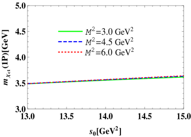
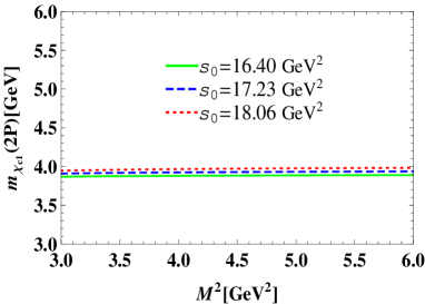
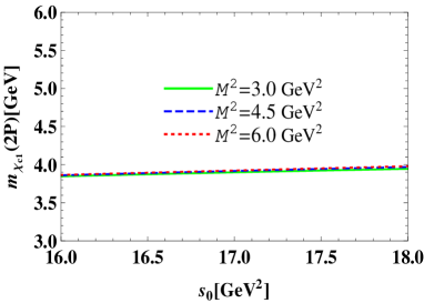
Figure 1: (Left panel) The mass of the meson $m_{\chi_{c1}(1P,2P)}$ as a function of the Borel parameter $M^{2}$ for fixed $s_{0}$, and (Right panel) the continuum threshold $s_{0}$ for fixed $M^{2}$.

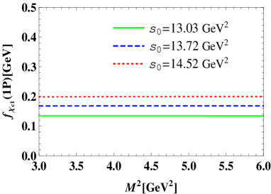
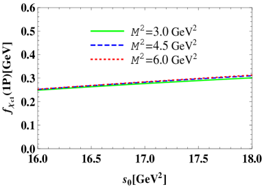
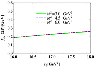
Figure 2: (Left panel) The dependence of the decay constant $f_{\chi_{c1}(1P,2P)}$ on the Borel mass parameter at chosen values of $s_{0}$, and (Right panel) on the $s_{0}$ for fixed $M^{2}$.

4 Concluding Remarks

We can summarize the present work by stating that a study of the $\chi_{c1}(1P)$ and $\chi_{c1}(2P)$ states has been carried out by employing QCD sum rules method, where in calculations terms up to dimension-8 have been computed. We adopted interpolating currents for $\chi_{c1}(1P)$ and $\chi_{c1}(2P)$ charmonia with quantum numbers $J^{PC}=1^{++}$. The mass and decay constant of the ground-state meson $\chi_{c1}(1P)$ and its first radial excitation $\chi_{c1}(2P)$ have been extracted from the corresponding QCDSR.

As is seen, our results obtained for the mass of $\chi_{c1}(2P)$ state by treating it as a first excited state of $\chi_{c1}(1P)$ is smaller than the mass of the $\chi_{c1}(4140)$ with a $~{}16.78\%$ difference. If we compare it to the $X(3872)$ particle, there is a mass difference of about $~{}9.22\%$. However the dominant idea on these particles in the literature that $X(3872)$ and $\chi_{c1}(4140)$ are probably exotic particles. Our mass value which we found as a result of calculations is very close to the $X(3940)$ particle. But we still don’t know the quantum numbers of this state. Also the QCD sum rule predictions for the mass and decay constants extracted in the present work by handling the interpolating current suffer from the large uncertainties. Anyhow such errors are inherent in the sum rule calculations, and are inevitable part of the whole picture. Therefore precise determination of the fundamental properties of charmonia is very important to explain the differences between experimental data and theoretical predictions. We hope that the theoretical studies and more sensitive experimental data will clarify our knowledge on this issue. To determine these hadronic parameters is also an important issue for the completion of the hadron spectrum. So these study can provide information and clues on the identification of the XYZ mesons. Our results may favorable in resolving the long-standing puzzle of determining the observed P-wave state, and also the interpretation of the enigmatic $X(3872)$ and $\chi_{c1}(4140)$ state [8].

Finally the charmonia are essential research area both at the running and projected in many large-scale experiments such as Belle, BESIII, LHC, BaBar and FAIR. The upcoming high precision data from BESIII, LHCb, Belle and BaBar as well as from the future detectors BelleII and PANDA will allow us to deeply understand the spectrum of the excited states and also the nature of the exotics.

Appendix A Spectral Density

The last explicit form of the perturbative part of the spectral density Eq. (13)

$$\rho^{\mathrm{Pert.}}(s)=\frac{1}{\pi^{2}}\Bigg{(}\frac{m_{c}^{2}}{s}+\frac{1}{8}\Bigg{)}\sqrt{s(s-4m_{c}^{2})}$$ (18)

The nonperturbative part of the spectral density Eq.  (13) is determined by the formula corresponding to the dimension four ($\rho_{4}$), six ($\rho_{6}$) and eight ($\rho_{8}$), respectively:

$$\rho^{\mathrm{Nonpert.}}(s) = \Big{\langle}\frac{\alpha_{s}G^{2}}{\pi}\Big{\rangle}\int_{0}^{1}~{}\rho^{\mathrm{(4)}}(z,s)~{}dz$$ (19)

$$+ \Big{\langle}g_{s}^{3}G^{3}\Big{\rangle}\int_{0}^{1}~{}\rho^{\mathrm{(6)}}(z,s)~{}dz$$

$$+ \Big{\langle}\frac{\alpha_{s}G^{2}}{\pi}\Big{\rangle}^{2}\int_{0}^{1}~{}\rho^{\mathrm{(8)}}(z,s)~{}dz.$$

In Eq. (19) the functions $~{}\rho_{4}(z,s),\ ~{}\rho_{6}(z,s)$ and $~{}\rho_{8}(z,s)$ have the explicit forms:

$$~{}\rho^{\mathrm{(4)}}(z,s) = \frac{1}{24r^{2}}\Big{[}3r^{2}(s-\varphi)+[m_{c}^{2}(3+9r)+sr^{2}]$$

$$\times \delta^{(1)}(s-\varphi)+m_{c}^{2}s(1-2z)^{2}\delta^{(2)}(s-\varphi)\Big{]},$$

$$~{}\rho^{\mathrm{(6)}}(z,s) = \frac{1}{15\cdot 2^{9}\pi^{2}r^{5}}\Bigg{\{}12\delta^{(1)}(s-\varphi)r^{3}[1+5r(1+r)]$$ (21)

$$+ 2r^{2}\delta^{(2)}(s-\varphi)\Big{[}27m_{c}^{2}[1+5r(1+r)]+2sr$$

$$\times [3+r(19+27r)]\Big{]}+r\delta^{(3)}(s-\varphi)\Big{[}-15m_{c}^{4}$$

$$\times [1+5r(1+r)]+6m_{c}^{2}sr[3+r(23+39r)]$$

$$+ s^{2}r^{3}(8+27r)]\Big{]}-\delta^{(4)}(s-\varphi)\Big{[}2m_{c}^{6}[1+5r$$

$$\times (1+r)]+m_{c}^{4}sr[7+r(39+47r)]-r^{5}s^{3}$$

$$- 6m_{c}^{2}r^{3}s^{2}(1-2z)^{2}\Big{]}\Bigg{\}}$$

and

$$~{}\rho^{\mathrm{(8)}}(z,s) = -\frac{1}{2^{4}\cdot 3^{3}r^{2}}m_{c}^{2}\pi^{2}\Big{[}6r\delta^{(3)}(s-\varphi)+\delta^{(5)}(s-\varphi)$$

$$\times s(m_{c}^{2}+rs)+\delta^{(4)}(s-\varphi)[m_{c}^{2}+2s(1+3r)]\Big{]}$$

where we use the following notations

$$\ r=z(z-1),\ \ \varphi=\frac{m_{c}^{2}}{z(1-z)}.$$ (23)

In the above expressions the Dirac delta function $\ \delta^{(n)}(s-\varphi)$ is defined as

$$\delta^{(n)}(s-\varphi)=\frac{d^{n}}{ds^{n}}\delta(s-\varphi).$$ (24)

References

References

• [1] Godfrey S and Olsen S L 2008 Ann. Rev. Nucl. Part. Sci. 58 51
• [2] Chen H X, Chen W, Liu X and Zhu S L 2016 Phys. Rept. 639 1
• [3] Tanabashi M et al. (Particle Data Group) 2018 Phys. Rev. D 98 030001
• [4] Hanhart C 2018 Int. J. Mod. Phys. Conf. Ser. 46 1860004
• [5] Gui L C, Lu L S, L Q F and Zhong X H 2018 Phys. Rev. D 98, 1, 016010
• [6] Pakhlov P et al. [Belle Collaboration], 2008 Phys. Rev. Lett.  100, 202001
• [7] Abe Ket al. [Belle Collaboration], 2007 Phys. Rev. Lett.  98, 082001
• [8] Zhou Z Y and Xiao Z 2017 Phys. Rev. D 96, 5, 054031 Erratum:[Phys. Rev. D 96, 9, 099905]
• [9] Godfrey S and Isgur N 1985 Phys. Rev. D 32 189
• [10] D’Souza P P, Bhat M, Monteiro A P and Vijaya Kumar K B 2017 Properties of Low-Lying Charmonium States in a Phenomenological Approach  arXiv:1703.10413 [hep-ph]
• [11] Achasov N N and Rogozina E V 2015 Mod. Phys. Lett. A 30, 33, 1550181
• [12] Wang T H and Wang G L 2011 Phys. Lett. B 697 233
• [13] Aubert B et al. [BaBar Collaboration] 2009 Phys. Rev. Lett. 102 132001
• [14] Bhardwaj V et al. [Belle Collaboration] 2011 Phys. Rev. Lett. 107 091803
• [15] De Fazio F 2012 PoS HQL 2012 001
• [16] Li B Q, Meng C and Chao K T 2009 Phys. Rev. D 80 014012
• [17] Zhou Z Y and Xiao Z 2014 Eur. Phys. J. A 50, 10, 165
• [18] Anisovich V V, Dakhno L G, Matveev M A, Nikonov V A and Sarantsev A V 2007 Phys. Atom. Nucl. 70 364
• [19] Beveren E V and Rupp G, arXiv:0906.2278 [hep-ph].
• [20] Swanson E S, 2015 Phys. Rev. D 91, 3, 034009
• [21] Agaev S S, Azizi K and Sundu H, 2017 Phys. Rev. D 95, 11, 114003
• [22] Turkan A and Dag H, arXiv:1705.02587 [hep-ph].
• [23] Stancu F 2010 J. Phys. G 37, 075017
• [24] Aaij R et al. [LHCb Collaboration] 2017 Phys. Rev. Lett. 118, 2, 022003
• [25] Aaij R et al. [LHCb Collaboration] 2017 Phys. Rev. D 95, 1, 012002
• [26] Liu X H 2017 Phys. Lett. B 766, 117
• [27] Ebert D, Faustov R N and Galkin V O 2010 Phys. Part. Nucl. 41, 931
• [28] Aaij R. et al. [LHCb Collaboration] 2012 Phys. Rev. D 85, 091103
• [29] Shifman M A, Vainshtein A I and Zakharov V I 1979 Nucl. Phys. B 147 385
• [30] Shifman M A, Vainshtein A I and Zakharov V I 1979 Nucl. Phys. B 147 448
• [31] Reinders L J, Rubinstein H and Yazaki S 1985 Phys. Rept. 127 1
• [32] Azizi K and Sungu J Y arXiv:1711.04288 [hep-ph].
• [33] Agaev S S, Azizi K and Sundu H 2017 Phys. Rev. D 96, 3, 034026
• [34] Agaev S S, Azizi K and Sundu H 2017 Eur. Phys. J. C 77, 6, 395
• [35] Narison S. 2010 Phys. Lett. B 693, 559 Erratum: [Phys. Lett. B 705, 544 (2011)]
• [36] Veliev E V, Azizi K, Sundu H and Kaya G 2014 Rom. J. Phys. 59, Number 1-2, 140
• [37] Palameta A, Harnett D and Steele T G, arXiv:1805.04230 [hep-ph].
• [38] Blank M and Krassnigg A 2011 Phys. Rev. D 84, 096014
• [39] Ebert D, Faustov R N and Galkin V O 2011 Eur. Phys. J. C 71 1825
• [40] Sonnenschein J and Weissman D 2017 Nucl. Phys. B 920, 319
• [41] Radford S F and Repko W W 2007 Phys. Rev. D 75 074031
• [42] Cao L, Yang Y C and Chen H 2012 Few Body Syst. 53, 327
• [43] Segovia J, Entem D R, Fernandez F and Hernandez E 2013 Int. J. Mod. Phys. E 22 1330026
• [44] Rui Z 2018 Phys. Rev. D 97, 3, 033001
• [45] Luchinsky D A V 2018 Charmonia Production in $W\to(c\bar{c})D_{s}^{(*)}$ Decays  arXiv:1801.08998 [hep-ph]
• [46] Munoz J H and Quintero N 2011 Rev. Mex. Fis. E 57, 1, 57