Spatio-temporal Edge Service Placement: A Bandit Learning Approach

Lixing Chen, ,  Jie Xu, ,  Shaolei Ren, ,  Pan Zhou,  L. Chen and J. Xu are with Department of Electrical and Computer Engineering, University of Miami, USA. S. Ren is with Department of Electrical and Computer Engineering, University of California, Riverside, USA. P. Zhou is with School of EIC, Huazhong University of Science and Technology, China.
Abstract

Shared edge computing platforms deployed at the radio access network are expected to significantly improve quality of service delivered by Application Service Providers (ASPs) in a flexible and economic way. However, placing edge service in every possible edge site by an ASP is practically infeasible due to the ASP’s prohibitive budget requirement. In this paper, we investigate the edge service placement problem of an ASP under a limited budget, where the ASP dynamically rents computing/storage resources in edge sites to host its applications in close proximity to end users. Since the benefit of placing edge service in a specific site is usually unknown to the ASP a priori, optimal placement decisions must be made while learning this benefit. We pose this problem as a novel combinatorial contextual bandit learning problem. It is “combinatorial” because only a limited number of edge sites can be rented to provide the edge service given the ASP’s budget. It is “contextual” because we utilize user context information to enable finer-grained learning and decision making. To solve this problem and optimize the edge computing performance, we propose SEEN, a Spatial-temporal Edge sErvice placemeNt algorithm. Furthermore, SEEN is extended to scenarios with overlapping service coverage by incorporating a disjunctively constrained knapsack problem. In both cases, we prove that our algorithm achieves a sublinear regret bound when it is compared to an oracle algorithm that knows the exact benefit information. Simulations are carried out on a real-world dataset, whose results show that SEEN significantly outperforms benchmark solutions.

I Introduction

Mobile cloud computing (MCC) supports mobile applications in resource-constrained mobile devices by offloading computation-demanding tasks to the resource-rich remote cloud. Intelligent personal assistant applications are perhaps the most popular applications that rely on MCC, where the speech recognition engine that uses advanced machine learning technologies to function resides in the cloud server. Nowadays, mobile applications such as virtual/augmented reality and mobile gaming are becoming even more data-hungry, latency-sensitive and location-aware. For example, Google Lens is a real-time image recognition application that can pull up the right information (e.g. restaurant reviews and menus) in an interactive and responsive way as the user points his/her smartphone camera to objects (e.g. a restaurant) when passing by. However, as these applications become more prevalent, ensuring high quality of service (QoS) becomes very challenging due to the backbone network congestion, delay and expensive bandwidth [1].

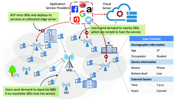
To address these challenges, mobile edge computing (MEC) [2] has recently been proposed. The key idea of MEC is to move the computation resources to the logical edge of the Internet, thereby enabling analytics and knowledge generation to occur closer to the data sources. Such an edge service provisioning scenario is no longer a mere vision, but becoming a reality. Vapor IO [3] has launched Project Volutus [4] to deliver shared edge computing services via a network of micro data centers deployed in cellular tower sites. In a recent white paper [5], Intel envisions that its smart cell platform will allow mobile operators to sell IT real-estate at the radio access network and to monetize their most valuable assets without compromising any of the network features. It is anticipated that Application Service Providers (ASPs) will soon be able to rent computation resources in such shared edge computing platforms in a flexible and economic way. Fig. 1 illustrates how the Google Lens application can leverage the shared edge computing platform to improve QoS.

Refer to caption
Figure 1: Mobile Edge Computing for Google Lens. In MCC (upper side), the image/video is sent to cloud server for processing via backbone Internet and incur large transmission latency; In MEC (lower side), the service is deployed at edge server collocated at the access point, and hence the image/video only needs to be sent to edge server for processing via one-hope wireless connection, which enables quick response.

While provisioning edge service in every possible edge site (i.e. base station) can deliver the best QoS, it is practically infeasible, especially for small and starting ASPs, due to the prohibitive budget requirement. In common business practice, an ASP has a budget on the operation expenses in mind and desires the best performance within the budget [6]. This means that an ASP will only be able to place edge services in a limited number of edge sites and hence, where to rent edge computation resources must be judiciously decided to improve QoS under the limited budget.

Deciding the optimal edge service placement policy faces significant challenges due to information uncertainty in both spatial and temporal domains. Firstly, the benefit of edge service provisioning primarily depends on the service demand of users, which can vary considerably across different sites. However, the demand pattern is usually unknown to the ASP before deploying edge service in a particular site, and may also vary substantially after frequent application updates. Because the demand pattern can only be observed at sites where the edge service is deployed, how to make the optimal tradeoff between exploration (i.e. to place edge service in unknown sites to learn the user demand pattern) and exploitation (i.e. to place edge service at high-demanding sites to maximize ASP utility) is a key challenge. Secondly, even in the same site, the service demand varies over time depending on who are currently in the mobile cell, what their preferences are, what mobile devices they use, time and other environmental variables. Collectively, this information is called the context information. Incorporating this valuable information into the edge service placement decision making, in addition to the plain number of devices, is likely to improve the overall system performance but is challenging because the context space can be huge. Learning for each specific context is nearly impossible due to the limited number of context occurrences. A promising approach is to group similar contexts so that learning can be carried out on the context-group level. However, how to group contexts in a way that enables both fast and effective learning demands for a careful design.

In this paper, we study the spatial-temporal edge service placement problem of an ASP under a limited budget and propose an efficient learning algorithm, called SEEN (Spatial-temporal Edge sErvice placemeNt), to optimize the edge computing performance. SEEN does not assume a priori knowledge about users’ service demand. Rather, it learns the demand pattern in an online fashion by observing the realized demand in sites where edge service is provisioned and uses this information to make future edge service placement decisions. In particular, SEEN is location-aware as it uses information only in the local area for each base station and is context-aware as it utilizes user context information to make edge service placement decisions.

The spatial-temporal edge service placement problem is posed as a novel Contextual Combinatorial Multi-armed Bandit (CC-MAB) problem [7] (see more detailed literature review in Section II). We analytically bound the loss due to learning, termed regret, of SEEN compared to an oracle benchmark that knows precisely the user demand pattern a priori. A sublinear regret bound is proved, which not only implies that SEEN produces an asymptotically optimal edge service placement policy but also provides finite-time performance guarantee. The proposed algorithm is further extended to scenarios with overlapping service coverage. In this case, a disjunctively constrained knapsack problem is incorporated into the framework of SEEN to deal with the service demand coupling caused by the coverage overlapping among cells. We prove that the sublinear regret bound still holds. To evaluate the performance of SEEN, we carry out extensive simulations on a real-world dataset on mobile application user demand [8], whose results show that SEEN significantly outperforms benchmark algorithms.

The rest of this paper is organized as follows. Section II reviews related works. Section III presents the system model and formulates the problem. Section IV designs SEEN and analyzes its performance. Section V extends SEEN to the overlapping coverage scenario. Section VI presents the simulation results, followed by the conclusion in Section VII.

II Related Work

Mobile edge computing has attracted much attention in recent years [9, 10]. Many prior studies focus on computation offloading, concerning what/when/how to offload users’ workload from their devices to the edge servers or the cloud. Various works have studied different aspects of this problem, considering e.g. stochastic task arrivals [11, 12], energy efficiency [13, 14], collaborative offloading [15, 16], etc. However, these works focus on the optimization problem after certain edge services have been provisioned at the Internet edge. By contrast, this paper focuses on how to place edge service among many possible sites in an edge system.

Service placement in edge computing has been studied in many contexts in the past. Considering content delivery as a service, many prior works study placing content replicas in traditional content delivery networks (CDNs) [17] and, more recently, in wireless caching systems such as small cell networks [18]. Early works addressed the centralized cases where the demand profile is static or time invariant, and dynamic service placement in geographically distributed clouds is studied in [19] in the presence of demand and resource dynamics. Our prior works [20, 21] investigate collaborative service placement to improve the efficiency of edge resource utilization by enabling cooperation among edge servers. However, these works assume that the service demand is known a priori whereas the service demand pattern in our problem has to be learned over time. A learning-based content caching algorithm for a wireless caching node was recently developed in [22], which also takes a contextual bandit learning approach similar to ours. However, it considers the caching policies (i.e. which content to cache) in a single caching site whereas we aim to determine where to place edge service among multiple edge sites, which may have to maintain distinct context spaces. Importantly, we also consider the coupled decisions among multiple sites due to the possible overlapping coverage while content files in [22] are treated independently.

MAB algorithms have been widely studied to address the critical tradeoff between exploration and exploitation in sequential decision making under uncertainty [7]. The basic MAB setting concerns with learning the single optimal action among a set of candidate actions of a priori unknown rewards by sequentially trying one action each time and observing its realized noisy reward [23, 24]. Combinatorial bandits extends the basic MAB by allowing multiple-play each time (i.e. choosing multiple edge sites under a budget in our problem) [25, 26, 27] and contextual bandits extends the basic MAB by considering the context-dependent reward functions [28, 29, 30]. While both combinatorial bandits and contextual bandits problems are already much more difficult than the basic MAB problem, this paper tackles the even more difficult CC-MAB problem. Recently, a few other works [31, 32] also started to study CC-MAB problems. However, these works make strong assumptions that are not suitable for our problem. For instance, [31, 32] assume that the reward of an individual action is a linear function of the contexts. [22] is probably the most related work that investigates contextual and combinatorial MAB for proactive caching. However, our work has many key differences from [22]. First, [22] considers CC-MAB for a single learner (a caching station) and maintains a common context space for all users. By contrast, our paper considers a multi-learner case, where each learner (i.e. SBS) learns the demand pattern of users within its service range. More importantly, we allow each SBS to maintain a distinct location-specific context space and collect different context information of connected users according to the user’s preference. Second, while [22] considers a bandit learning problem for a fixed size of content items, we allow our algorithm to deal with infinitely large user set. Third, we further consider an overlapped edge network and address the decision coupling among edge sites due to overlapped coverage.

III System Model

III-A Edge System and Edge Service Provisioning

We consider a heterogeneous network consisting of N𝑁N small cells (SCs), indexed by 𝒩𝒩\mathcal{N}, and a macro base station (MBS). Each SC has a small-cell base station (SBS) equipped with a shared edge computing platform and thus is an edge site that can be used to host edge services for ASPs. The MBS provides ubiquitous radio coverage and access to the cloud server in case edge computing is not accessible. SBSs (edge sites) provide Software-as-a-Service (SaaS) to ASPs, managing computation/storage resources (e.g. CPU, scheduling, etc.) to ensure end-to-end QoS, while the ASP maintains its own user data, serving as a middleman between end users and SaaS Providers. As such, SBSs charge the ASP for the amount of time the edge service is rented. Fig. 2 gives an illustration for the considered scenario.
Refer to caption
Figure 2: Illustration of context-aware edge service provisioning

Specifically, computation and storage resource allocation in SBSs can be realized by containerization techniques [33], e.g., Dockers and Kubernetes [34]. The key advantage of containerization over the virtual machine technology is that it incurs much lower system overhead and much shorter launch time. For example, each SBS can set up a Docker Registry to store Dock images (i.e. a package that encapsulates the running environment of an application) locally. When the SBS is chosen to host the ASP’s application, it will pull up the Docker image for the corresponding application and configure the container in seconds [35]. Without loss of generality, this paper focuses on the service placement for one application. Due to the limited budget, the ASP can only rent up to b(b<N)𝑏𝑏𝑁b(b<N) SBSs, where we assume for simplicity that all SBSs charge the same price for a unit time.

TABLE I: Nomenclature
Variable Description
𝒩𝒩\mathcal{N} a set of total N𝑁N SBSs
b𝑏b the budget of ASP
𝒮tsuperscript𝒮𝑡\mathcal{S}^{t} the set of SBSs selected in slot t𝑡t
𝒮tsuperscript𝒮absent𝑡\mathcal{S}^{*t} Oracle solution in slot t𝑡t
tsuperscript𝑡\mathcal{M}^{t} user population in slot t𝑡t
ntsubscriptsuperscript𝑡𝑛\mathcal{M}^{t}_{n} users covered by SBS n𝑛n
dmtsubscriptsuperscript𝑑𝑡𝑚d^{t}_{m} service demand of user m𝑚m in slot t𝑡t
λ𝜆\lambda input data size of one task
η𝜂\eta required CPU cycles for one task
Qn,mtsubscriptsuperscript𝑄𝑡𝑛𝑚Q^{t}_{n,m} the delay of completing one task for user m𝑚m at SBS n𝑛n
u~n,mtsubscriptsuperscript~𝑢𝑡𝑛𝑚\tilde{u}^{t}_{n,m} the delay reduction of one task
𝒳nsubscript𝒳𝑛\mathcal{X}_{n} context space maintained by SBS n𝑛n
Dnsubscript𝐷𝑛D_{n} dimension of context space monitored by SBS n𝑛n
𝒫n,Tsubscript𝒫𝑛𝑇\mathcal{P}_{n,T} partition created on context space 𝒳nsubscript𝒳𝑛\mathcal{X}_{n}
xn,msubscript𝑥𝑛𝑚x_{n,m} user m𝑚m’s context observed by SBS n𝑛n, xn,m𝒳nsubscript𝑥𝑛𝑚subscript𝒳𝑛x_{n,m}\in\mathcal{X}_{n}
𝑿tsuperscript𝑿𝑡{\boldsymbol{X}}^{t} contexts of all users in slot t𝑡t, 𝑿t=(xn,mt)mn,n𝒩superscript𝑿𝑡subscriptsubscriptsuperscript𝑥𝑡𝑛𝑚formulae-sequence𝑚subscript𝑛𝑛𝒩{\boldsymbol{X}}^{t}=(x^{t}_{n,m})_{m\in\mathcal{M}_{n},n\in\mathcal{N}}
μ(x)𝜇𝑥\mu(x) expected service demand for a user with context x𝑥x
d^(p)^𝑑𝑝\hat{d}(p) demand estimation for users with context in hypercube p𝑝p

The operational timeline is discretized into time slots. In each time slot t𝑡t, ASP chooses a set of SBSs 𝒮t𝒩superscript𝒮𝑡𝒩\mathcal{S}^{t}\in\mathcal{N}, where |𝒮t|bsuperscript𝒮𝑡𝑏|\mathcal{S}^{t}|\leq b, for application deployment. This decision is referred to as the (edge) service placement decision in the rest of this paper. Let t=1,,Mtsuperscript𝑡1superscript𝑀𝑡\mathcal{M}^{t}={1,\dots,M^{t}} be the user population served by the entire network in time slot t𝑡t and let nttsubscriptsuperscript𝑡𝑛superscript𝑡\mathcal{M}^{t}_{n}\subseteq\mathcal{M}^{t} be the user population covered by SBS n𝑛n. The user population in the considered network can vary across time slots because of the user mobility. Users can also move within a time slot but we assume that the User-SBS association remains the same within a time slot for simplicity. We consider that the service placement decisions are made on the scale of minutes so that frequent reconfiguration of edge services is avoided while the temporal variation of user population is largely captured.

We will first consider the case where the service areas of SBSs are non-overlapping and then consider the case with overlapping service areas in Section V. In the non-overlapping case, if SBS n𝑛n is chosen by the ASP to host the application in time slot t𝑡t, i.e. n𝒮t𝑛superscript𝒮𝑡n\in\mathcal{S}^{t}, then user mnt𝑚subscriptsuperscript𝑡𝑛m\in\mathcal{M}^{t}_{n} in its coverage can offload data to SBS n𝑛n for edge computing. Otherwise, users in SBS n𝑛n’s coverage have to offload data to the cloud (via the MBS) for cloud computing.

III-B ASP Utility Model

The ASP derives utility by deploying edge computing services. On the one hand, the ASP has a larger utility if the edge computing service is deployed in areas where the service demand is larger as more users can enjoy a higher QoS. Let dmtsubscriptsuperscript𝑑𝑡𝑚d^{t}_{m} (in terms of the number of tasks) be the service demand of user m𝑚m in time slot t𝑡t, which is unknown a priori at the edge service placement decision time, and the service demand of all users in the network is collected in 𝒅t=(dmt)mtsuperscript𝒅𝑡subscriptsubscriptsuperscript𝑑𝑡𝑚𝑚superscript𝑡{\boldsymbol{d}}^{t}=(d^{t}_{m})_{m\in\mathcal{M}^{t}}. On the other hand, the ASP derives a larger utility if edge computing service is deployed in areas where edge computing performs much better than cloud computing. In this paper, we use delay as a performance metric of edge/cloud computing. Since we focus on a single application, we assume that tasks have same input data size λ𝜆\lambda (in bits) and required CPU cycles η𝜂\eta.

III-B1 Delay by Edge Computing

If the task of user mnt𝑚subscriptsuperscript𝑡𝑛m\in\mathcal{M}^{t}_{n} is processed by SBS n𝑛n at the edge, then the delay consists of the wireless transmission delay and edge computation delay. The achievable wireless uplink transmission rate between user m𝑚m and SBS n𝑛n can be calculated according to the Shannon capacity: rn,mt=Wlog2(1+PmuHn,mt/(N0+I))subscriptsuperscript𝑟𝑡𝑛𝑚𝑊subscript21subscriptsuperscript𝑃𝑢𝑚subscriptsuperscript𝐻𝑡𝑛𝑚subscript𝑁0𝐼r^{t}_{n,m}=W\log_{2}\left(1+P^{u}_{m}H^{t}_{n,m}/(N_{0}+I)\right), where W𝑊W is the channel bandwidth, Pmusubscriptsuperscript𝑃𝑢𝑚P^{u}_{m} is the transmission power of user m𝑚m’ device, Hn,mtsubscriptsuperscript𝐻𝑡𝑛𝑚H^{t}_{n,m} is the uplink channel gain between user m𝑚m and SBS n𝑛n in time slot t𝑡t, N0subscript𝑁0N_{0} is the noise power and I𝐼I is the interference. Therefore, the transmission delay Qn,mtx,tsubscriptsuperscript𝑄tx𝑡𝑛𝑚Q^{\text{tx},t}_{n,m} of user m𝑚m for sending a task (i.e. λ𝜆\lambda bits of input data) to SBS n𝑛n is Qn,mtx,t=λ/rn,mtsubscriptsuperscript𝑄tx𝑡𝑛𝑚𝜆subscriptsuperscript𝑟𝑡𝑛𝑚Q^{\text{tx},t}_{n,m}=\lambda/r^{t}_{n,m}. We assume that the data size of the task result is small. Hence the downlink transmission delay is neglected. The computation delay depends on the computation workload and the edge server’s CPU frequency. To simplify our analysis, we assume that the edge server of SBS n𝑛n processes tasks at its maximum CPU speed fnsubscript𝑓𝑛f_{n}. Therefore, the computation delay for one task is η/fn𝜂subscript𝑓𝑛\eta/f_{n}. Overall, the delay of processing user m𝑚m’s one task at the edge site of SBS n𝑛n is Qn,mt=λ/rn,mt+η/fnsubscriptsuperscript𝑄𝑡𝑛𝑚𝜆subscriptsuperscript𝑟𝑡𝑛𝑚𝜂subscript𝑓𝑛Q^{t}_{n,m}=\lambda/r^{t}_{n,m}+\eta/f_{n}.

III-B2 Delay by Cloud Computing

If the task of user mnt𝑚subscriptsuperscript𝑡𝑛m\in\mathcal{M}^{t}_{n} is processed in the cloud, then the delay consists of the wireless transmission delay, the backbone Internet transmission delay and the cloud computation delay. The wireless transmission delay can be computed similarly as in the edge computing case by first calculating the transmission rate r0,mtsubscriptsuperscript𝑟𝑡0𝑚r^{t}_{0,m} between user m𝑚m and the MBS. The cloud computing delay can also be calculated similarly using the cloud server’s CPU frequency f0subscript𝑓0f_{0}. However, compared to edge computing, cloud computing incurs an additional transmission delay since the data has to travel across the backbone Internet. Let vtsuperscript𝑣𝑡v^{t} be the backbone transmission rate and htsuperscript𝑡h^{t} be the round trip time in time slot t𝑡t, then an additional transmission delay λ/vt+ht𝜆superscript𝑣𝑡superscript𝑡\lambda/v^{t}+h^{t} is incurred. Overall, the delay of processing user m𝑚m’s one task in the cloud is Q0,mt=λ/r0,mt+η/f0+(λ/vt+ht)subscriptsuperscript𝑄𝑡0𝑚𝜆subscriptsuperscript𝑟𝑡0𝑚𝜂subscript𝑓0𝜆superscript𝑣𝑡superscript𝑡Q^{t}_{0,m}=\lambda/r^{t}_{0,m}+\eta/f_{0}+(\lambda/v^{t}+h^{t}).

Taking into account the service demand and the possible delay reduction provided by edge computing. The utility of ASP when taking service placement decision 𝒮tsuperscript𝒮𝑡\mathcal{S}^{t} in time slot t𝑡t is:

Ut(𝒅t,𝒮t)=n𝒮tmntu~n,mtdmtsuperscript𝑈𝑡superscript𝒅𝑡superscript𝒮𝑡subscript𝑛superscript𝒮𝑡subscript𝑚subscriptsuperscript𝑡𝑛subscriptsuperscript~𝑢𝑡𝑛𝑚subscriptsuperscript𝑑𝑡𝑚\displaystyle U^{t}({\boldsymbol{d}}^{t},\mathcal{S}^{t})=\sum_{n\in\mathcal{S}^{t}}\sum_{m\in\mathcal{M}^{t}_{n}}\tilde{u}^{t}_{n,m}d^{t}_{m} (1)

where u~n,mtQ0,mtQn,mtsubscriptsuperscript~𝑢𝑡𝑛𝑚subscriptsuperscript𝑄𝑡0𝑚subscriptsuperscript𝑄𝑡𝑛𝑚\tilde{u}^{t}_{n,m}\triangleq Q^{t}_{0,m}-Q^{t}_{n,m} is the delay reduction for user m𝑚m if it is served by SBS n𝑛n. The above utility function assumes that the tasks from a user are independent, i.e., the utility of a task is immediately realized upon the receival of its own results and does not need to wait until all tasks of the user are completed. Therefore, the ASP concerns the service delay for each individual tasks of users instead of measuring the delay for completing all the tasks of a user in time slot t𝑡t. Similar utility functions are also widely adopted in the existing literature [36]. The utility is essentially a weighted service popularity, where the weight is the reduced delay by deploying edge services compared to cloud computing. Clearly, other weights, such as task/user priority, can also be easily incorporated into our framework.

Remarks on delay model: We use simple models to capture the service delay incurred by task transmission and processing. Note that other communication models (e.g., Massive MIMO) and computing models (e.g., queuing system) can also be applied depending on the practical system configuration. In these cases, the delay reduction should be recalculated accordingly. The algorithm proposed in this paper is compatible with other delay models as long as tasks’ delay reduction u~n,mtsubscriptsuperscript~𝑢𝑡𝑛𝑚\tilde{u}^{t}_{n,m} can be obtained.

III-C Context-Aware Edge Service Provisioning

A user’s service demand depends on many factors, which are collectively referred to as the context. For example, relevant factors can be demographic factors (e.g., age111Young people are more interested in Game Apps as shown in [8]., gender), equipment type (e.g. smartphone, tablet), equipment status (e.g., battery levels 222A device with low battery level tend to offload computational tasks to edge servers [14]. ), as well as external environment factors (e.g., location, time, and events). This categorization is clearly not exhaustive and the impact of each single context dimension on the service demand is unknown a priori. These context information helps the ASP to understand the demand pattern of connected users and provide the edge service efficiently. Our algorithm will learn to discover the underlying connection between such context and users’ service demand pattern (see an example of such a connection in Figure 5(c) based on a real-world dataset in Section VI), which will be discussed in detail in the next subsection III-D, thereby facilitating the service placement decision making.

At each SBS, a context monitor periodically gathers context information by accessing information about currently connected users and optionally by collecting additional information from external sources (e.g. social media platforms). However, collecting the user context sometimes faces a concern known as the privacy disclosure management [37], which decides when, where, and what personal information can be revealed. The central notion behind privacy disclosure management is that people disclose different versions of personal information to different entities under different conditions [37]. Therefore, the service area of an SBS (e.g. business building, apartment complex, and plaza) may influence users’ privacy preference [38, 39] and hence determine what context information an SBS can access. To capture this feature, we allow each SBS to maintain its own user context space depending on its local users’ privacy preference. This results in the heterogeneity of context spaces maintained by SBSs. Note that the context spaces of different SBSs may be completely different, partially overlapping or exactly the same. Our model captures the most general cases and all SBSs having the same context space is a special case of ours. Formally, let Dnsubscript𝐷𝑛D_{n} be the number of context dimensions monitored by SBS n𝑛n for its connected users. The monitored context space of SBS n𝑛n is denoted by 𝒳nsubscript𝒳𝑛\mathcal{X}_{n} which is assumed to be bounded and hence can be denoted as 𝒳n=[0,1]Dnsubscript𝒳𝑛superscript01subscript𝐷𝑛\mathcal{X}_{n}=[0,1]^{D_{n}} without loss of generality. Let xn,mt𝒳n,mntformulae-sequencesubscriptsuperscript𝑥𝑡𝑛𝑚subscript𝒳𝑛for-all𝑚subscriptsuperscript𝑡𝑛x^{t}_{n,m}\in\mathcal{X}_{n},\forall m\in\mathcal{M}^{t}_{n} be the context vector of user m𝑚m monitored by SBS n𝑛n in time slot t𝑡t. The context vectors of all users connected to SBS n𝑛n are collected in 𝒙nt=(xn,mt)mntsubscriptsuperscript𝒙𝑡𝑛subscriptsubscriptsuperscript𝑥𝑡𝑛𝑚𝑚subscriptsuperscript𝑡𝑛{\boldsymbol{x}}^{t}_{n}=(x^{t}_{n,m})_{m\in\mathcal{M}^{t}_{n}}.

III-D Problem Formulation

Now, we formulate the edge service placement problem as a CC-MAB learning problem. In each time slot t𝑡t, the edge system operates sequentially as follows: (i) each SBS n𝒩𝑛𝒩n\in\mathcal{N} monitors the context xn,mt𝒳nsubscriptsuperscript𝑥𝑡𝑛𝑚subscript𝒳𝑛x^{t}_{n,m}\in\mathcal{X}_{n} of all connected users mnt𝑚subscriptsuperscript𝑡𝑛m\in\mathcal{M}^{t}_{n} and collects the context information in 𝒙nt=(xn,mt)mntsubscriptsuperscript𝒙𝑡𝑛subscriptsubscriptsuperscript𝑥𝑡𝑛𝑚𝑚subscriptsuperscript𝑡𝑛{\boldsymbol{x}}^{t}_{n}=(x^{t}_{n,m})_{m\in\mathcal{M}^{t}_{n}}. (ii) The ASP chooses a set of SBSs 𝒮tsuperscript𝒮𝑡\mathcal{S}^{t} with |𝒮t|=bsuperscript𝒮𝑡𝑏|\mathcal{S}^{t}|=b based on the context information collected by all SBSs 𝑿t=(𝒙nt)n𝒩superscript𝑿𝑡subscriptsubscriptsuperscript𝒙𝑡𝑛𝑛𝒩{\boldsymbol{X}}^{t}=({\boldsymbol{x}}^{t}_{n})_{n\in\mathcal{N}} in the current time slot, and the knowledge learned from previous time slots. (iii) The users are informed about the current service placement decision 𝒮tsuperscript𝒮𝑡\mathcal{S}^{t}. Till the end of the current time slot, users connected to SBSs in 𝒮tsuperscript𝒮𝑡\mathcal{S}^{t} can request edge computing service from these SBSs. (iv) At the end of the current slot, the service demand dmtsubscriptsuperscript𝑑𝑡𝑚d^{t}_{m} of user mnt𝑚subscriptsuperscript𝑡𝑛m\in\mathcal{M}^{t}_{n} served by SBS n𝒮t𝑛superscript𝒮𝑡n\in\mathcal{S}^{t} is observed.

The service demand dmtsubscriptsuperscript𝑑𝑡𝑚d^{t}_{m} of user mnt𝑚subscriptsuperscript𝑡𝑛m\in\mathcal{M}^{t}_{n} with context xn,mt𝒳nsubscriptsuperscript𝑥𝑡𝑛𝑚subscript𝒳𝑛x^{t}_{n,m}\in\mathcal{X}_{n} is a random variable with a unknown distribution. We denote this random service demand by d(xn,mt)𝑑subscriptsuperscript𝑥𝑡𝑛𝑚d(x^{t}_{n,m}) and its expected value by μ(xn,mt)=𝔼[d(xn,mt)]𝜇subscriptsuperscript𝑥𝑡𝑛𝑚𝔼delimited-[]𝑑subscriptsuperscript𝑥𝑡𝑛𝑚\mu(x^{t}_{n,m})=\mathbb{E}[d(x^{t}_{n,m})]. The random service demand is assumed to take values in [0,dmax]0superscript𝑑[0,d^{\max}], where dmaxsuperscript𝑑d^{\max} is the maximum possible number of tasks a user can have in one time slot. The service demand (d(xn,mt))n𝒩,mntsubscript𝑑subscriptsuperscript𝑥𝑡𝑛𝑚formulae-sequence𝑛𝒩𝑚subscriptsuperscript𝑡𝑛\left(d(x^{t}_{n,m})\right)_{n\in\mathcal{N},m\in\mathcal{M}^{t}_{n}} is assumed to be independent, i.e., the service demands of users served by an SBS are independent of each other. Moreover, each d(xn,mt)𝑑subscriptsuperscript𝑥𝑡𝑛𝑚d(x^{t}_{n,m}) is assumed to be independent of the past service provision decisions and previous service demands.

The goal of the ASP is to rent at most b𝑏b SBSs for edge service hosting in order to maximize the expected utility up to a finite time horizon T𝑇T. Based on the system utility defined in (1), the edge service placement problem can be formally written as:

P1:max(𝒮t)t=1,,TP1:subscriptsubscriptsuperscript𝒮𝑡𝑡1𝑇\displaystyle\textbf{P1:}~{}~{}\max_{(\mathcal{S}^{t})_{t=1,\dots,T}} t=1Tn𝒮tmntu~n,mtμ(xn,mt)superscriptsubscript𝑡1𝑇subscript𝑛superscript𝒮𝑡subscript𝑚subscriptsuperscript𝑡𝑛subscriptsuperscript~𝑢𝑡𝑛𝑚𝜇subscriptsuperscript𝑥𝑡𝑛𝑚\displaystyle~{}~{}\sum_{t=1}^{T}\sum_{n\in\mathcal{S}^{t}}\sum_{m\in\mathcal{M}^{t}_{n}}\tilde{u}^{t}_{n,m}\mu(x^{t}_{n,m}) (2a)
s.t. |𝒮t|b,𝒮t𝒩,t.formulae-sequencesuperscript𝒮𝑡𝑏superscript𝒮𝑡𝒩for-all𝑡\displaystyle~{}~{}|\mathcal{S}^{t}|\leq b,\mathcal{S}^{t}\subseteq\mathcal{N},~{}\forall t. (2b)

III-E Oracle Benchmark Solution

Before presenting our bandit learning algorithm, we first give an oracle benchmark solution to P1 by assuming that the ASP had a priori knowledge about context-specific service demand, i.e., for an arbitrary user m𝑚m with context vector xn,m𝒳n,mn,n𝒩formulae-sequencesubscript𝑥𝑛𝑚subscript𝒳𝑛formulae-sequencefor-all𝑚subscript𝑛𝑛𝒩x_{n,m}\in\mathcal{X}_{n},\forall m\in\mathcal{M}_{n},n\in\mathcal{N}, the ASP would know the expected demand μ(xn,m)𝜇subscript𝑥𝑛𝑚\mu(x_{n,m}). It is obvious that P1 can be decoupled into T𝑇T independent sub-problems, one for each time slot t𝑡t:

P2max𝒮tP2subscriptsuperscript𝒮𝑡\displaystyle\textbf{P2}~{}~{}\max_{\mathcal{S}^{t}} n𝒮tmntu~n,mtμ(xn,mt)subscript𝑛superscript𝒮𝑡subscript𝑚subscriptsuperscript𝑡𝑛subscriptsuperscript~𝑢𝑡𝑛𝑚𝜇subscriptsuperscript𝑥𝑡𝑛𝑚\displaystyle~{}~{}\sum_{n\in\mathcal{S}^{t}}\sum_{m\in\mathcal{M}^{t}_{n}}\tilde{u}^{t}_{n,m}\mu(x^{t}_{n,m}) (3a)
s.t. |𝒮t|b,𝒮t𝒩.formulae-sequencesuperscript𝒮𝑡𝑏superscript𝒮𝑡𝒩\displaystyle~{}~{}|\mathcal{S}^{t}|\leq b,\mathcal{S}^{t}\subseteq\mathcal{N}. (3b)

The optimal solution to the subproblem P2 in time slot t𝑡t can be easily derived in a running time of O(|N|log(N))𝑂𝑁𝑁O(|N|\log(N)) as follows: Given the contexts 𝑿tsuperscript𝑿𝑡{\boldsymbol{X}}^{t} of connected users in time slot t𝑡t, the optimal solution is to select the b𝑏b highest ranked SBSs (top-b𝑏b SBSs) {n1(𝑿t),n2(𝑿t),,nb(𝑿t)}𝒩subscriptsuperscript𝑛1superscript𝑿𝑡subscriptsuperscript𝑛2superscript𝑿𝑡subscriptsuperscript𝑛𝑏superscript𝑿𝑡𝒩\left\{n^{*}_{1}({\boldsymbol{X}}^{t}),n^{*}_{2}({\boldsymbol{X}}^{t}),\dots,n^{*}_{b}({\boldsymbol{X}}^{t})\right\}\in\mathcal{N} which, for j=1,,b𝑗1𝑏j=1,\dots,b, satisfy:

nj(𝑿t)argmaxn𝒩\k=1j1nk(𝑿t)mntu~n,mtμ(xn,mt)subscriptsuperscript𝑛𝑗superscript𝑿𝑡subscriptargmax𝑛\𝒩subscriptsuperscript𝑗1𝑘1subscriptsuperscript𝑛𝑘superscript𝑿𝑡subscript𝑚subscriptsuperscript𝑡𝑛subscriptsuperscript~𝑢𝑡𝑛𝑚𝜇subscriptsuperscript𝑥𝑡𝑛𝑚\displaystyle n^{*}_{j}({\boldsymbol{X}}^{t})\in\operatorname*{arg\,max}_{n\in\mathcal{N}\backslash\bigcup^{j-1}_{k=1}n^{*}_{k}({\boldsymbol{X}}^{t})}~{}\sum_{m\in\mathcal{M}^{t}_{n}}\tilde{u}^{t}_{n,m}\mu(x^{t}_{n,m}) (4)

We denote by 𝒮t=k=1bnk(𝑿t)superscript𝒮absent𝑡subscriptsuperscript𝑏𝑘1subscriptsuperscript𝑛𝑘superscript𝑿𝑡\mathcal{S}^{*t}=\bigcup^{b}_{k=1}n^{*}_{k}({\boldsymbol{X}}^{t}) the optimal oracle solution in time slot t𝑡t. Consequently, the collection (𝒮t)t=1Tsuperscriptsubscriptsuperscript𝒮absent𝑡𝑡1𝑇\left(\mathcal{S}^{*t}\right)_{t=1}^{T} is the optimal oracle solution to P1.

However, in practice, the ASP does not have a priori knowledge about the service demand. In this case, ASP cannot simply solve P1 as described above, since the expected service demands are unknown. Hence, an ASP has to learn the expected service demand over time by observing the users’ contexts and service demand. For this purpose, the ASP has to make a trade-off between deploying edge services at SBSs where little information is available (exploration) and SBSs which it believes to yield the highest demands (exploitation). In each time slot, the ASP’s service placement decision depends on the history of choices in the past and observed user context. An algorithm which maps the decision history to the current service placement decision is called a learning algorithm. The oracle solution (𝒮t)t=1Tsuperscriptsubscriptsuperscript𝒮absent𝑡𝑡1𝑇\left(\mathcal{S}^{*t}\right)_{t=1}^{T}, is used as a benchmark to evaluate the loss of learning. The regret of learning with respect to the oracle solution is given by

R(T)=t=1T(n𝒮tmnt𝔼[u~n,mtd(xn,mt)]n𝒮tmnt𝔼[u~n,mtd(xn,mt)])𝑅𝑇superscriptsubscript𝑡1𝑇subscript𝑛superscript𝒮absent𝑡subscript𝑚subscriptsuperscript𝑡𝑛𝔼delimited-[]subscriptsuperscript~𝑢𝑡𝑛𝑚𝑑subscriptsuperscript𝑥𝑡𝑛𝑚subscript𝑛superscript𝒮𝑡subscript𝑚subscriptsuperscript𝑡𝑛𝔼delimited-[]subscriptsuperscript~𝑢𝑡𝑛𝑚𝑑subscriptsuperscript𝑥𝑡𝑛𝑚\displaystyle R(T)=\sum_{t=1}^{T}\left(\sum_{n\in\mathcal{S}^{*t}}\sum_{m\in\mathcal{M}^{t}_{n}}\mathbb{E}\left[\tilde{u}^{t}_{n,m}d(x^{t}_{n,m})\right]-\sum_{n\in\mathcal{S}^{t}}\sum_{m\in\mathcal{M}^{t}_{n}}\mathbb{E}\left[\tilde{u}^{t}_{n,m}d(x^{t}_{n,m})\right]\right) (5)

Here, the expectation is taken with respect to the decisions made by the learning algorithm and the distributions of users’ service demand.

IV CC-MAB for Edge Service Placement

In order to place edge services at the most beneficial SBSs given the context information of currently connected users, the ASP should learn context-specific service demand for the connected users. According to the above formulation, this problem is a combinatorial contextual MAB problem and we propose an algorithm called SEEN (Spatio-temporal Edge sErvice placemeNt) for learning the context-specific service demand and solving P1.

IV-A Algorithm Structure

Our SEEN algorithm is based on the assumption that users with similar context information covered by the same SBS will have similar service demand. This is a natural assumption in practice, which can be exploited together with the users’ context information to learn future service provisioning decisions. Our algorithm starts by partitioning the context space maintained by each SBS uniformly into small hypercubes, i.e. splitting the entire context space into parts of similar contexts. Then, an SBS learns the service demand independently in each hypercube of similar contexts. Based on the observed context information of all connected users and a certain control function, the algorithm is interspersed with exploration phases and exploitation phases. In the exploration phases, ASP chooses a random set of SBSs for edge service placement. These phases are needed to learn the local users’ service demand patterns of SBSs which have not been chosen often before. Otherwise, the algorithm is in an exploitation phase, in which it chooses SBSs which on average gave the highest utility when rented in previous time slots with similar user contexts. After choosing the new set of SBSs, the algorithm observes the users’ true service demand at the end of every time slot. In this way, the algorithm learns context-specific service demand over time. The design challenge lies in how to partition the context space and how to determine when to explore/exploit.

The pseudo-code of SEEN is presented in Algorithm 1. In the initialization phase, SEEN creates a partition 𝒫n,Tsubscript𝒫𝑛𝑇\mathcal{P}_{n,T} for each SBS n𝑛n given the time horizon T𝑇T, which splits the context space 𝒳n=[0,1]Dnsubscript𝒳𝑛superscript01subscript𝐷𝑛\mathcal{X}_{n}=[0,1]^{D_{n}} into (hn,T)Dnsuperscriptsubscript𝑛𝑇subscript𝐷𝑛(h_{n,T})^{D_{n}} sets and these sets are given by Dnsubscript𝐷𝑛D_{n}-dimensional hypercubes of identical size 1hn,T××1hn,T1subscript𝑛𝑇1subscript𝑛𝑇\dfrac{1}{h_{n,T}}\times\dots\times\dfrac{1}{h_{n,T}}. Here, hn,Tsubscript𝑛𝑇h_{n,T} is an input parameter which determines the number of hypercubes in the partition. Additionally, SBS n𝑛n keeps a counter Cnt(p)subscriptsuperscript𝐶𝑡𝑛𝑝C^{t}_{n}(p) for each hypercube p𝒫n,T𝑝subscript𝒫𝑛𝑇p\in\mathcal{P}_{n,T} indicating the number of times that a user with context from hypercube p𝑝p connects to SBS n𝑛n when it was rented to host edge service up to time slot t𝑡t. Moreover, SEEN also keeps an estimated demand d^(p)^𝑑𝑝\hat{d}(p) for each hypercube p𝒫n,T𝑝subscript𝒫𝑛𝑇p\in\mathcal{P}_{n,T}. Let nt(p)subscriptsuperscript𝑡𝑛𝑝\mathcal{E}^{t}_{n}(p) be the set of observed service demand of users with context from set p𝒫n,T𝑝subscript𝒫𝑛𝑇p\in\mathcal{P}_{n,T} up to time slot t𝑡t. Then, the estimated demand of users with context from set p𝑝p is given by the sample mean:

d^(p)=1|nt(p)|dnt(p)d^𝑑𝑝1subscriptsuperscript𝑡𝑛𝑝subscript𝑑subscriptsuperscript𝑡𝑛𝑝𝑑\displaystyle\hat{d}(p)=\dfrac{1}{|\mathcal{E}^{t}_{n}(p)|}\sum_{d\in\mathcal{E}^{t}_{n}(p)}d (6)

where |nt(p)|subscriptsuperscript𝑡𝑛𝑝|\mathcal{E}^{t}_{n}(p)| equals Cnt(p)subscriptsuperscript𝐶𝑡𝑛𝑝C^{t}_{n}(p). Notice that the set nt(p)subscriptsuperscript𝑡𝑛𝑝\mathcal{E}^{t}_{n}(p) does not need be stored since the estimated demand d^(p)^𝑑𝑝\hat{d}(p) can be updated based on nt1(p),Cnt1(p)subscriptsuperscript𝑡1𝑛𝑝subscriptsuperscript𝐶𝑡1𝑛𝑝\mathcal{E}^{t-1}_{n}(p),C^{t-1}_{n}(p), and observed demands in time slot t𝑡t.

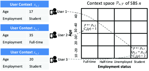
In each time slot t𝑡t, SBS n𝑛n first observes the currently connected users ntsubscriptsuperscript𝑡𝑛\mathcal{M}^{t}_{n} and their context 𝒙n=(xn,mt)mntsubscript𝒙𝑛subscriptsubscriptsuperscript𝑥𝑡𝑛𝑚𝑚subscriptsuperscript𝑡𝑛{\boldsymbol{x}}_{n}=(x^{t}_{n,m})_{m\in\mathcal{M}^{t}_{n}}. For each piece of context information xn,mtsubscriptsuperscript𝑥𝑡𝑛𝑚x^{t}_{n,m}, SEEN determines the hypercube pn,mt𝒫n,Tsubscriptsuperscript𝑝𝑡𝑛𝑚subscript𝒫𝑛𝑇p^{t}_{n,m}\in\mathcal{P}_{n,T} to which the xn,mtsubscriptsuperscript𝑥𝑡𝑛𝑚x^{t}_{n,m} belongs, i.e., xn,mtpn,mtsubscriptsuperscript𝑥𝑡𝑛𝑚subscriptsuperscript𝑝𝑡𝑛𝑚x^{t}_{n,m}\in p^{t}_{n,m} holds. The collection of these hypercubes is given by 𝒑nt=(pn,mt)mntsubscriptsuperscript𝒑𝑡𝑛subscriptsubscriptsuperscript𝑝𝑡𝑛𝑚𝑚subscriptsuperscript𝑡𝑛{\boldsymbol{p}}^{t}_{n}=(p^{t}_{n,m})_{m\in\mathcal{M}^{t}_{n}} for each SBS n𝒩𝑛𝒩n\in\mathcal{N}, and 𝑷t=(𝒑nt)n𝒩superscript𝑷𝑡subscriptsubscriptsuperscript𝒑𝑡𝑛𝑛𝒩{\boldsymbol{P}}^{t}=({\boldsymbol{p}}^{t}_{n})_{n\in\mathcal{N}} for the whole network. Fig. 3 offers a simple illustration of the context hypercubes and the update of counters with a 2-D context space assuming three users are currently connected to SBS n𝑛n.

Refer to caption
Figure 3: Illustration of context space and counters

Then the algorithm is in either an exploration phase or an exploitation phase. In order to determine the correct phase in the current time slot, the algorithm checks if there are SBSs that have not been explored sufficiently often. For this purpose, the set of under-explored SBSs 𝒩ue,tsuperscript𝒩ue𝑡\mathcal{N}^{\text{ue},t} are obtained in each time slot as follows:

𝒩ue,t={n:n𝒩,mnt,Cnt(pn,mt)<Kn(t)}superscript𝒩ue𝑡conditional-set𝑛formulae-sequence𝑛𝒩formulae-sequence𝑚subscriptsuperscript𝑡𝑛subscriptsuperscript𝐶𝑡𝑛subscriptsuperscript𝑝𝑡𝑛𝑚subscript𝐾𝑛𝑡\displaystyle\mathcal{N}^{\text{ue},t}=\{n:n\in\mathcal{N},\exists~{}m\in\mathcal{M}^{t}_{n},C^{t}_{n}(p^{t}_{n,m})<K_{n}(t)\} (7)

where Kn(t)subscript𝐾𝑛𝑡K_{n}(t) is a deterministic, monotonically increasing control function, which is an input to the algorithm and has to be set appropriately to balance the trade-off between exploration and exploitation. In the next subsection, we will design a control function that guarantees a good balance in terms of this trade-off.

Algorithm 1 Spatio-temporal Edge Service Provisioning (SEEN)
1:Input: T𝑇T, hn,Tsubscript𝑛𝑇h_{n,T}, Kn(t)subscript𝐾𝑛𝑡K_{n}(t).
2:Initialization create partition 𝒫n,Tsubscript𝒫𝑛𝑇\mathcal{P}_{n,T}; set Cn0(p)=0,p𝒫n,T,n𝒩formulae-sequencesubscriptsuperscript𝐶0𝑛𝑝0formulae-sequencefor-all𝑝subscript𝒫𝑛𝑇𝑛𝒩C^{0}_{n}(p)=0,\forall p\in\mathcal{P}_{n,T},n\in\mathcal{N};
3:for t=1,,T𝑡1𝑇t=1,\dots,T do
4:     SBS n𝒩𝑛𝒩n\in\mathcal{N} observe currently connected users ntsubscriptsuperscript𝑡𝑛\mathcal{M}^{t}_{n} and context 𝒙nt=(xn,mt)mntsubscriptsuperscript𝒙𝑡𝑛subscriptsubscriptsuperscript𝑥𝑡𝑛𝑚𝑚subscriptsuperscript𝑡𝑛{\boldsymbol{x}}^{t}_{n}=(x^{t}_{n,m})_{m\in\mathcal{M}^{t}_{n}};
5:     Find 𝒑nt=(pn,mt)mntsubscriptsuperscript𝒑𝑡𝑛subscriptsubscriptsuperscript𝑝𝑡𝑛𝑚𝑚subscriptsuperscript𝑡𝑛{\boldsymbol{p}}^{t}_{n}=(p^{t}_{n,m})_{m\in\mathcal{M}^{t}_{n}} such that xn,mtpn,mt𝒫n,T,n𝒩,mntformulae-sequencesubscriptsuperscript𝑥𝑡𝑛𝑚subscriptsuperscript𝑝𝑡𝑛𝑚subscript𝒫𝑛𝑇formulae-sequencefor-all𝑛𝒩𝑚subscriptsuperscript𝑡𝑛x^{t}_{n,m}\in p^{t}_{n,m}\in\mathcal{P}_{n,T},\forall n\in\mathcal{N},m\in\mathcal{M}^{t}_{n};
6:     Identify under-explored SBSs 𝒩ue,tsuperscript𝒩ue𝑡\mathcal{N}^{\text{ue},t} in (7) and let q=size(𝒩ue,t)𝑞sizesuperscript𝒩ue𝑡q=\text{size}(\mathcal{N}^{\text{ue},t});
7:     if 𝒩ue,tsuperscript𝒩ue𝑡\mathcal{N}^{\text{ue},t}\neq\emptyset then: \triangleright Exploration
8:         if qb𝑞𝑏q\geq b then: 𝒮tsuperscript𝒮𝑡absent\mathcal{S}^{t}\leftarrow randomly rent b𝑏b SBSs from 𝒩ue,tsuperscript𝒩ue𝑡\mathcal{N}^{\text{ue},t}.
9:         else: 𝒮tsuperscript𝒮𝑡absent\mathcal{S}^{t}\leftarrow rent q𝑞q SBSs from 𝒩ue,tsuperscript𝒩ue𝑡\mathcal{N}^{\text{ue},t}, (bq)𝑏𝑞(b-q) SBSs from (n^j(𝑿t))j=1(bq)superscriptsubscriptsubscript^𝑛𝑗superscript𝑿𝑡𝑗1𝑏𝑞\left(\hat{n}_{j}({\boldsymbol{X}}^{t})\right)_{j=1}^{(b-q)} in (8);          
10:     else: 𝒮tsuperscript𝒮𝑡absent\mathcal{S}^{t}\leftarrow rent b𝑏b from (n^j(𝑿t))j=1bsuperscriptsubscriptsubscript^𝑛𝑗superscript𝑿𝑡𝑗1𝑏\left(\hat{n}_{j}({\boldsymbol{X}}^{t})\right)_{j=1}^{b} in (9); \triangleright Exploitation      
11:     Observe service demand dmsubscript𝑑𝑚d_{m} of user m𝑚m, mnt,n𝒮tformulae-sequencefor-all𝑚subscriptsuperscript𝑡𝑛for-all𝑛superscript𝒮𝑡\forall m\in\mathcal{M}^{t}_{n},\forall n\in\mathcal{S}^{t};
12:     for n𝒮t𝑛superscript𝒮𝑡n\in\mathcal{S}^{t} and mnt𝑚subscriptsuperscript𝑡𝑛m\in\mathcal{M}^{t}_{n} do \triangleright Demand estimation update
13:         Update estimated demand: d^(pn,mt)=d^(pn,mt)Cn(pn,mt)+dmCn(pn,mt)+1^𝑑subscriptsuperscript𝑝𝑡𝑛𝑚^𝑑subscriptsuperscript𝑝𝑡𝑛𝑚subscript𝐶𝑛subscriptsuperscript𝑝𝑡𝑛𝑚subscript𝑑𝑚subscript𝐶𝑛subscriptsuperscript𝑝𝑡𝑛𝑚1\hat{d}(p^{t}_{n,m})=\frac{\hat{d}(p^{t}_{n,m})C_{n}(p^{t}_{n,m})+d_{m}}{C_{n}(p^{t}_{n,m})+1};
14:         Update counters: Cn(pn,mt)=Cn(pn,mt)+1subscript𝐶𝑛subscriptsuperscript𝑝𝑡𝑛𝑚subscript𝐶𝑛subscriptsuperscript𝑝𝑡𝑛𝑚1C_{n}(p^{t}_{n,m})=C_{n}(p^{t}_{n,m})+1;      
15: The time indices of the counters Cn,ptsubscriptsuperscript𝐶𝑡𝑛𝑝C^{t}_{n,p} are dropped in Line 13 and 14 due to recursive update.

If the set of under-explored SBSs is non-empty, SEEN enters the exploration phase. Let q(t)𝑞𝑡q(t) be the number of under-explored SBSs. If the set of under-explored SBSs contains at least b𝑏b elements, i.e. q(t)>b𝑞𝑡𝑏q(t)>b, SEEN randomly rents b𝑏b SBSs from 𝒩ue,tsuperscript𝒩ue𝑡\mathcal{N}^{\text{ue},t}. If the number of under-explored SBS is less than b𝑏b, i.e. q(t)<b𝑞𝑡𝑏q(t)<b, it selects q(t)𝑞𝑡q(t) SBSs from 𝒩ue,tsuperscript𝒩ue𝑡\mathcal{N}^{\text{ue},t} and (bq(t))𝑏𝑞𝑡(b-q(t)) additional SBSs are selected. These additional SBSs are those that have the highest estimated demand:

n^jt(𝑿t)argmaxn𝒩\{𝒩ue,t,k=1j1n^kt(𝑿t)}mntu~n,md^(pn,mt).subscriptsuperscript^𝑛𝑡𝑗superscript𝑿𝑡subscriptargmax𝑛\𝒩superscript𝒩ue𝑡subscriptsuperscript𝑗1𝑘1subscriptsuperscript^𝑛𝑡𝑘superscript𝑿𝑡subscript𝑚subscriptsuperscript𝑡𝑛subscript~𝑢𝑛𝑚^𝑑subscriptsuperscript𝑝𝑡𝑛𝑚\displaystyle\hat{n}^{t}_{j}({\boldsymbol{X}}^{t})\in\operatorname*{arg\,max}_{n\in\mathcal{N}\backslash\{\mathcal{N}^{\text{ue},t},~{}\bigcup^{j-1}_{k=1}\hat{n}^{t}_{k}({\boldsymbol{X}}^{t})\}}~{}\sum_{m\in\mathcal{M}^{t}_{n}}\tilde{u}_{n,m}\hat{d}(p^{t}_{n,m}). (8)

If the set of SBSs defined by (8) is not unique, ties are broken arbitrarily. If the set of under-explored SBSs is empty, then the algorithm enters the exploitation phase, in which it selects b𝑏b SBSs that have the highest estimated demand, as defined below:

n^jt(𝑿t)argmaxn𝒩\k=1j1n^kt(𝑿t)mntu~n,md^(pn,mt).subscriptsuperscript^𝑛𝑡𝑗superscript𝑿𝑡subscriptargmax𝑛\𝒩subscriptsuperscript𝑗1𝑘1subscriptsuperscript^𝑛𝑡𝑘superscript𝑿𝑡subscript𝑚subscriptsuperscript𝑡𝑛subscript~𝑢𝑛𝑚^𝑑subscriptsuperscript𝑝𝑡𝑛𝑚\displaystyle\hat{n}^{t}_{j}({\boldsymbol{X}}^{t})\in\operatorname*{arg\,max}_{n\in\mathcal{N}\backslash\bigcup^{j-1}_{k=1}\hat{n}^{t}_{k}({\boldsymbol{X}}^{t})}~{}\sum_{m\in\mathcal{M}^{t}_{n}}\tilde{u}_{n,m}\hat{d}(p^{t}_{n,m}). (9)

Finally, each chosen SBS observes the received service demand from users at the end of time slot t𝑡t and then updates the estimated service demand and the counters for each hypercube.

IV-B Analysis of the Regret

Next, we give an upper performance bound of the proposed algorithm in term of the regret. The regret bound is derived based on the natural assumption that the expected service demands of users are similar in similar contexts. Because users’ preferences of service demand differ based on their context, it is plausible for SBSs to divide its user population into groups with similar context and similar preferences. This assumption is formalized by the following Hölder condition for each SBS.

Assumption 1 (Hölder Condition).

For an arbitrary SBS n𝒩𝑛𝒩n\in\mathcal{N}, there exists Ln>0subscript𝐿𝑛0L_{n}>0, αn>0subscript𝛼𝑛0\alpha_{n}>0 such that for any x,x𝒳n𝑥superscript𝑥subscript𝒳𝑛x,x^{\prime}\in\mathcal{X}_{n}, it holds that

|μ(x)μ(x)|Lnxxαn𝜇𝑥𝜇superscript𝑥subscript𝐿𝑛superscriptnorm𝑥superscript𝑥subscript𝛼𝑛\displaystyle|\mu(x)-\mu(x^{\prime})|\leq L_{n}\|x-x^{\prime}\|^{\alpha_{n}} (10)

where \|\cdot\| denotes the Euclidean norm in Dnsuperscriptsubscript𝐷𝑛\mathbb{R}^{D_{n}}.

We note that this assumption is needed for the analysis of the regret but SEEN can still be applied if it does not hold true. In that case, however, a regret bound might not be guaranteed. Under Assumption 1, the following Theorem shows that the regret of SEEN is sublinear in the time horizon T𝑇T, i.e. R(T)=O(Tγ)𝑅𝑇𝑂superscript𝑇𝛾R(T)=O(T^{\gamma}) with γ<1𝛾1\gamma<1. This regret bound guarantees that SEEN has an asymptotically optimal performance, since limTR(T)T=0subscript𝑇𝑅𝑇𝑇0\lim_{T\to\infty}\frac{R(T)}{T}=0 holds. This means that SEEN converges to the optimal edge service placement strategy used by the oracle solution. Specifically, the regret of SEEN can be bounded as follows for any finite time horizon T𝑇T.

Theorem 1 (Bound for R(T)𝑅𝑇R(T)).

Let Kn(t)=t2αn3αn+Dnlog(t)subscript𝐾𝑛𝑡superscript𝑡2subscript𝛼𝑛3subscript𝛼𝑛subscript𝐷𝑛𝑡K_{n}(t)=t^{\frac{2\alpha_{n}}{3\alpha_{n}+D_{n}}}\log(t) and hn,T=T13αn+Dnsubscript𝑛𝑇superscript𝑇13subscript𝛼𝑛subscript𝐷𝑛h_{n,T}=\lceil T^{\frac{1}{3\alpha_{n}+D_{n}}}\rceil. If SEEN is run with these parameters and Assumption 1 holds true, the leading order of the regret R(T)𝑅𝑇R(T) is O(bNu~maxMmaxdmax2Dn¯T2αn¯+Dn¯3αn¯+Dn¯log(T))𝑂𝑏𝑁superscript~𝑢superscript𝑀superscript𝑑superscript2subscript𝐷¯𝑛superscript𝑇2subscript𝛼¯𝑛subscript𝐷¯𝑛3subscript𝛼¯𝑛subscript𝐷¯𝑛𝑇O\left(bN\tilde{u}^{\max}M^{\max}d^{\max}2^{D_{\bar{n}}}T^{\frac{2\alpha_{\bar{n}}+D_{\bar{n}}}{3\alpha_{\bar{n}}+D_{\bar{n}}}}\log(T)\right), where n¯=argmaxn2αn+Dn3αn+Dn¯𝑛subscriptargmax𝑛2subscript𝛼𝑛subscript𝐷𝑛3subscript𝛼𝑛subscript𝐷𝑛\bar{n}=\operatorname*{arg\,max}_{n}\frac{2\alpha_{n}+D_{n}}{3\alpha_{n}+D_{n}}.

Proof.

See online Appendix A in [40]. ∎

Theorem 1 indicates that the regret bound achieved by the proposed SEEN algorithm is sublinear in the time horizon T𝑇T. Moreover, the bound is valid for any finite time horizon, thereby providing a bound on the performance loss for any finite number of service placement decision cycles. This can be used to characterize the convergence speed of the proposed algorithm. In the special case of b=1𝑏1b=1 and αn=α,Dn=D,nformulae-sequencesubscript𝛼𝑛𝛼subscript𝐷𝑛𝐷for-all𝑛\alpha_{n}=\alpha,D_{n}=D,\forall n, the considered CC-MAB problem reduces to the standard contextual MAB problem. In this case, the order of the regret is O~(T2α+D3α+D)~𝑂superscript𝑇2𝛼𝐷3𝛼𝐷\tilde{O}(T^{\frac{2\alpha+D}{3\alpha+D}}). We note that the regret bound, which although is still sublinear in T𝑇T, is loose when the budget b𝑏b is close to N𝑁N. Consider the special case of b=N𝑏𝑁b=N, SEEN actually is identical to the naive optimal service placement policy (i.e. choose all N𝑁N SBSs to deploy the edge service) and hence, the actual regret is 0. It is intuitive that when the budget b𝑏b is large, learning is not very much needed and hence the more challenging regime is when the budget b𝑏b is small (but not 1).

IV-C Complexity and Scalability

The memory requirements of SEEN is mainly determined by the counters and estimated context-specific demands kept by the SBSs. For each SBS n𝒩𝑛𝒩n\in\mathcal{N}, it keeps the counters Cn(p)subscript𝐶𝑛𝑝C_{n}(p) and estimated demand d^(p)^𝑑𝑝\hat{d}(p) for each hypercube in the partition 𝒫n,Tsubscript𝒫𝑛𝑇\mathcal{P}_{n,T}. If SEEN is run with the parameters in Theorem 1, the number of hypercubes is (hn,T)Dn=T13αn+DnDnsuperscriptsubscript𝑛𝑇subscript𝐷𝑛superscriptsuperscript𝑇13subscript𝛼𝑛subscript𝐷𝑛subscript𝐷𝑛(h_{n,T})^{D_{n}}=\lceil T^{\frac{1}{3\alpha_{n}+D_{n}}}\rceil^{D_{n}}. Hence, the required memory is sublinear in the time horizon T𝑇T. However, this means that when T𝑇T\to\infty, the algorithm would require infinite memory. Fortunately, in the practical implementations, SBS only needs to keep the counters of such hypercubes p𝑝p to which at least one of its connected users’ context vectors belongs. Hence the required number of counters that have to be kept is actually much smaller than the analytical requirement.

SEEN can be easily implemented with a large network without incurring a large overhead, since each SBS keeps counters and estimated user demands independently according to its maintained context space. At the beginning of each time slot, the ASP queries the SBSs about their status (explored or under-explored) and estimated utilities, and then chooses b𝑏b SBSs based on SEEN. Therefore, the number of SBSs does not complicate the algorithm much.

V Edge Service Placement for SBSs with Coverage Overlapping

So far we have considered the edge service placement problem for a set of non-overlapping SBSs. However, SBSs may be densely deployed in areas with large mobile traffic data and computation demand, which creates the overlapping of SBSs’ coverage. In this case, a user can be possibly served by multiple SBSs, and therefore whether a user’s service demand can be processed at the Internet edge is determined by the service availability at all reachable SBSs. This creates spatial coupling of service demand among overlapped SBSs, i.e., users observed by an SBS may send service requests to other nearby SBSs. Therefore, it is difficult for the ASP to optimize the service placement policies by considering the service availability at each SBS separately. In this section, we propose an algorithm SEEN-O which extends SEEN for small-cell networks with coverage overlapping.

V-A SBS Component and Component-wise Service Provisioning

We start by introducing the SBS components and component-wise decision. SEEN-O first constructs an undirected graph G=𝒩,𝐺𝒩G=\langle\mathcal{N},\mathcal{E}\rangle based on the small-cell network. Each SBS n𝒩𝑛𝒩n\in\mathcal{N} corresponds to a vertex in G𝐺G. For each pair of vertices i,j𝒩𝑖𝑗𝒩i,j\in\mathcal{N}, an edge ei,jsubscript𝑒𝑖𝑗e_{i,j}\in\mathcal{E} is added between them if and only if the service areas of the two SBSs have coverage overlapping. Based on the constructed graph G𝐺G, we give the definition of component as follows:

Definition 1 (Component).

A component of an undirected graph is a subgraph in which any two vertices are connected to each other by paths, and which is connected to no additional vertices.

By the definition of component, we know that a set of overlapped SBSs correspond to a component C𝒩𝐶𝒩C\subseteq\mathcal{N} in graph G𝐺G. Let 𝒞={C1,C2,,CK}𝒞subscript𝐶1subscript𝐶2subscript𝐶𝐾\mathcal{C}=\{C_{1},C_{2},\dots,C_{K}\} collect all K𝐾K components in graph G𝐺G. For an arbitrary component Ck𝒞subscript𝐶𝑘𝒞C_{k}\in\mathcal{C}, we define a set of component-wise decisions Zk={z:zCk,z}subscript𝑍𝑘conditional-set𝑧formulae-sequence𝑧subscript𝐶𝑘𝑧Z_{k}=\{z:z\subseteq C_{k},z\neq\emptyset\}, which collects all possible service placement decisions for SBSs in component Cksubscript𝐶𝑘C_{k}. The component-wise decision set Zksubscript𝑍𝑘Z_{k} can also be written as Zk={zk,1,zk,2,,zk,L}subscript𝑍𝑘subscript𝑧𝑘1subscript𝑧𝑘2subscript𝑧𝑘𝐿Z_{k}=\{z_{k,1},z_{k,2},\dots,z_{k,L}\}, where the total number of decisions in Zksubscript𝑍𝑘Z_{k} is given by the Bell number L=j=1|Ck|(|Ck|j)𝐿superscriptsubscript𝑗1subscript𝐶𝑘binomialsubscript𝐶𝑘𝑗L=\sum_{j=1}^{|C_{k}|}{|C_{k}|\choose j}. For an arbitrary component Cksubscript𝐶𝑘C_{k}, if a component-wise decision zk,lZksubscript𝑧𝑘𝑙subscript𝑍𝑘z_{k,l}\in Z_{k} is taken, then the ASP rents SBSs nzk,l𝑛subscript𝑧𝑘𝑙n\in z_{k,l} from the set of overlapping SBSs in Cisubscript𝐶𝑖C_{i}. Notice that the non-overlapping SBS network is a special case: for the components Cksubscript𝐶𝑘C_{k} containing only one SBS n𝑛n (i.e., non-overlapping SBS), its component-wise decision set Zksubscript𝑍𝑘Z_{k} contains only one element zk,1={n}subscript𝑧𝑘1𝑛z_{k,1}=\{n\}. Let 𝒵=k=1KZk𝒵subscriptsuperscript𝐾𝑘1subscript𝑍𝑘\mathcal{Z}=\bigcup^{K}_{k=1}Z_{k} be component-wise decision sets for the whole network. Fig. 4 provides a simple illustration of the SBS components and component-wise decisions.

Refer to caption
Figure 4: Illustration of SBS components and component-wise decisions. The component-wise decision set for the whole network is 𝒵={[1],[2],[3],[4],[2,3],[2,4],[3,4],[2,3,4]}𝒵delimited-[]1delimited-[]2delimited-[]3delimited-[]4232434234\mathcal{Z}=\left\{[1],[2],[3],[4],[2,3],[2,4],[3,4],[2,3,4]\right\}.

Instead of picking service placement decisions for individual SBSs separately, SEEN-O chooses component-wise decisions for components Ck𝒞subscript𝐶𝑘𝒞C_{k}\in\mathcal{C} due to the fact that service demand received by an SBS is jointly decided by the service availability at SBSs in the same component. Let Cksubscriptsubscript𝐶𝑘\mathcal{M}_{C_{k}} denote the users collaboratively served by SBSs in component Cksubscript𝐶𝑘C_{k}. For a user mCk𝑚subscriptsubscript𝐶𝑘m\in\mathcal{M}_{C_{k}}, it is able to request edge services from multiple SBSs in the component depending on the chosen component-wise decision zk,lZksubscript𝑧𝑘𝑙subscript𝑍𝑘z_{k,l}\in Z_{k}. Let Hn,mtsubscriptsuperscript𝐻𝑡𝑛𝑚H^{t}_{n,m} be the uplink channel gain between user m𝑚m and SBS nCk𝑛subscript𝐶𝑘n\in C_{k}. If SBS n𝑛n is not reachable for user m𝑚m, then Hn,mt=0subscriptsuperscript𝐻𝑡𝑛𝑚0H^{t}_{n,m}=0. Usually, users’ devices are energy-constrained and hence we assume that the service demand dmtsubscriptsuperscript𝑑𝑡𝑚d^{t}_{m} of user mCi𝑚subscriptsubscript𝐶𝑖m\in\mathcal{M}_{C_{i}} is offloaded to the SBS that has the best uplink channel condition among those that can provide edge service, namely argmaxnzk,lHn,mtsubscript𝑛subscript𝑧𝑘𝑙subscriptsuperscript𝐻𝑡𝑛𝑚\arg\max_{n\in z_{k,l}}H^{t}_{n,m}. In this way, users incur the least transmission energy consumption 333Our algorithm is also compatible with other User-SBS association strategies. The association decision amsubscript𝑎𝑚a_{m} of user m𝑚m can be formally written as:

am(z)=argmaxnCkHn,mt1{nz},mCk,zZk.formulae-sequencesubscript𝑎𝑚𝑧subscriptargmax𝑛subscript𝐶𝑘subscriptsuperscript𝐻𝑡𝑛𝑚1𝑛𝑧formulae-sequence𝑚subscriptsubscript𝐶𝑘𝑧subscript𝑍𝑘\displaystyle a_{m}(z)=\operatorname*{arg\,max}_{n\in C_{k}}~{}H^{t}_{n,m}\cdot\textbf{1}\{n\in z\},m\in\mathcal{M}_{C_{k}},z\in Z_{k}. (11)

Note that the uplink channel conditions can be easily monitored by the users, and we also assume that the users report monitored channel conditions to all reachable SBSs. Therefore, the association decisions of user mCk𝑚subscriptsubscript𝐶𝑘m\in\mathcal{M}_{C_{k}} are known to the SBSs given the component-wise decision z𝑧z. Let n(Ck,z)subscript𝑛subscript𝐶𝑘𝑧\mathcal{M}_{n}(C_{k},z) be the users connected to SBS nz,zCkformulae-sequence𝑛𝑧𝑧subscript𝐶𝑘n\in z,z\subseteq C_{k}, we have:

n(Ck,z)={m:mCk,am(z)=n},nCk,zZk.formulae-sequencesubscript𝑛subscript𝐶𝑘𝑧conditional-set𝑚formulae-sequence𝑚subscriptsubscript𝐶𝑘subscript𝑎𝑚𝑧𝑛formulae-sequence𝑛subscript𝐶𝑘𝑧subscript𝑍𝑘\displaystyle\mathcal{M}_{n}(C_{k},z)=\{m:m\in\mathcal{M}_{C_{k}},a_{m}(z)=n\},n\in C_{k},z\in Z_{k}. (12)

In addition, for each SBS n𝑛n we define u~n(z)=mn(Ck,z)u~n,mμ(xn,mt)subscript~𝑢𝑛𝑧subscript𝑚subscript𝑛subscript𝐶𝑘𝑧subscript~𝑢𝑛𝑚𝜇subscriptsuperscript𝑥𝑡𝑛𝑚\tilde{u}_{n}(z)=\sum_{m\in\mathcal{M}_{n}(C_{k},z)}\tilde{u}_{n,m}\mu(x^{t}_{n,m}), where u~n,msubscript~𝑢𝑛𝑚\tilde{u}_{n,m} is the delay improvement of user m𝑚m as defined in (1). Let 𝒮zt𝒵subscriptsuperscript𝒮𝑡𝑧𝒵\mathcal{S}^{t}_{z}\subseteq\mathcal{Z} be the component-wise decisions chosen by the ASP. Notice that the ASP can only draw at most one component-wise decision zZk𝑧subscript𝑍𝑘z\in Z_{k} for each component Cksubscript𝐶𝑘C_{k}. Then, we have the edge service placement problem as follows:

P3:max(𝒮zt)t=1,,TP3:subscriptsubscriptsuperscriptsubscript𝒮𝑧𝑡𝑡1𝑇\displaystyle\textbf{P3:}~{}~{}~{}\max_{(\mathcal{S}_{z}^{t})_{t=1,\dots,T}} t=1Tz𝒮ztnzu~n(z)superscriptsubscript𝑡1𝑇subscript𝑧superscriptsubscript𝒮𝑧𝑡subscript𝑛𝑧subscript~𝑢𝑛𝑧\displaystyle~{}~{}\sum_{t=1}^{T}\sum_{z\in\mathcal{S}_{z}^{t}}\sum_{n\in z}\tilde{u}_{n}(z) (13a)
s.t. z𝒮zt|z|b,tsubscript𝑧subscriptsuperscript𝒮𝑡𝑧𝑧𝑏for-all𝑡\displaystyle\sum_{z\in\mathcal{S}^{t}_{z}}|z|\leq b,~{}~{}\forall~{}t (13b)
z𝒮zt1{zZk}1,k,tsubscript𝑧subscriptsuperscript𝒮𝑡𝑧1𝑧subscript𝑍𝑘1for-all𝑘for-all𝑡\displaystyle\sum_{z\in\mathcal{S}^{t}_{z}}{\textbf{1}\{z\in Z_{k}\}}\leq 1,~{}~{}\forall~{}k,\forall~{}t (13c)

where (13b) is the budget constraint for the ASP and (13c) indicates that only one component-wise decision can be selected for each component.

V-B Disjunctively Constrained Knapsack Problem

Now, we consider an oracle solution for P3. Similarly, P3 can be decoupled into T𝑇T sub-problems.Yet, the solution for each sub-problem cannot be easily derived as in (4) due to different costs incurred by different component-wise decisions and, more importantly, the conflicts among component-wise decisions in (13c). The per-slot subproblem of P3 can be formulated as a Knapsack problem with Conflict Graphs (KCG), which is also referred to as disjunctively constrained knapsack problem. The conflict graph Gc=𝒵,csubscript𝐺𝑐𝒵subscript𝑐G_{c}=\langle\mathcal{Z},\mathcal{E}_{c}\rangle is defined based on the component-wise decisions: Each component-wise decision z𝒵𝑧𝒵z\in\mathcal{Z} corresponds to a vertex in Gcsubscript𝐺𝑐G_{c}. For an arbitrary pair of vertices z,z𝒵𝑧superscript𝑧𝒵z,z^{\prime}\in\mathcal{Z}, add an edge e(z,z)c𝑒𝑧superscript𝑧subscript𝑐e(z,z^{\prime})\in\mathcal{E}_{c} between z𝑧z and zsuperscript𝑧z^{\prime} if there exist a component-wise decision set Zk𝒵subscript𝑍𝑘𝒵Z_{k}\in\mathcal{Z} such that z,zZk𝑧superscript𝑧subscript𝑍𝑘z,z^{\prime}\in Z_{k}.

In the following, we convert P3 to a standard formulation of the KCG problem. For each z𝒵𝑧𝒵z\in\mathcal{Z}, we define a tuple (pz,cz,yz)subscript𝑝𝑧subscript𝑐𝑧subscript𝑦𝑧(p_{z},c_{z},y_{z}) where pz=nzu~n(z)subscript𝑝𝑧subscript𝑛𝑧subscript~𝑢𝑛𝑧p_{z}=\sum_{n\in z}\tilde{u}_{n}(z) is the profit of choosing component-wise decision z𝑧z, czsubscript𝑐𝑧c_{z} is the cost of decision z𝑧z which equals |z|𝑧|z|, and yz{0,1}subscript𝑦𝑧01y_{z}\in\{0,1\} indicates whether the decision z𝑧z is taken or not. Then, a KCG problem equivalent to P3 can be written as:

P3-KCG::P3-KCGabsent\displaystyle\textbf{P3-KCG}:~{}~{}~{} maxz𝒵pzyzsubscript𝑧𝒵subscript𝑝𝑧subscript𝑦𝑧\displaystyle\max~{}\sum_{z\in\mathcal{Z}}p_{z}y_{z} (14a)
s.t. z𝒵czyzbsubscript𝑧𝒵subscript𝑐𝑧subscript𝑦𝑧𝑏\displaystyle\sum_{z\in\mathcal{Z}}c_{z}y_{z}\leq b (14b)
yz+yz<1,z,z𝒵,e(z,z)cformulae-sequencesubscript𝑦𝑧subscript𝑦superscript𝑧1for-all𝑧formulae-sequencesuperscript𝑧𝒵for-all𝑒𝑧superscript𝑧subscript𝑐\displaystyle y_{z}+y_{z^{\prime}}<1,\forall z,z^{\prime}\in\mathcal{Z},\forall e(z,z^{\prime})\in\mathcal{E}_{c} (14c)
yz{0,1},z𝒵formulae-sequencesubscript𝑦𝑧01for-all𝑧𝒵\displaystyle y_{z}\in\{0,1\},\forall z\in\mathcal{Z} (14d)

The above problem is an NP-hard combinatorial optimization problem. Existing works have proposed various algorithms, including heuristic solutions[41] and exact solutions [42] to solve KCG. In the simulation we employ the Branch-and-Bound algorithm [43] to solve P3-KCG.

Algorithm 2 SEEN-O
1:Input: T𝑇T, hn,Tsubscript𝑛𝑇h_{n,T}, Kn(t)subscript𝐾𝑛𝑡K_{n}(t).
2:Initialization context partition: 𝒫n,Tsubscript𝒫𝑛𝑇\mathcal{P}_{n,T}; set Cn0(p)=0,p𝒫n,T,n𝒩formulae-sequencesubscriptsuperscript𝐶0𝑛𝑝0formulae-sequencefor-all𝑝subscript𝒫𝑛𝑇𝑛𝒩C^{0}_{n}(p)=0,\forall p\in\mathcal{P}_{n,T},n\in\mathcal{N};
3:for t=1,,T𝑡1𝑇t=1,\dots,T do
4:     SBS n𝒩𝑛𝒩n\in\mathcal{N} observe currently connected users ntsubscriptsuperscript𝑡𝑛\mathcal{M}^{t}_{n} and context 𝒙nt=(xn,mt)mntsubscriptsuperscript𝒙𝑡𝑛subscriptsubscriptsuperscript𝑥𝑡𝑛𝑚𝑚subscriptsuperscript𝑡𝑛{\boldsymbol{x}}^{t}_{n}=(x^{t}_{n,m})_{m\in\mathcal{M}^{t}_{n}};
5:     Find 𝒑nt=(pn,mt)mntsubscriptsuperscript𝒑𝑡𝑛subscriptsubscriptsuperscript𝑝𝑡𝑛𝑚𝑚subscriptsuperscript𝑡𝑛{\boldsymbol{p}}^{t}_{n}=(p^{t}_{n,m})_{m\in\mathcal{M}^{t}_{n}} such that xn,mtpn,mt𝒫n,T,n𝒩,mntformulae-sequencesubscriptsuperscript𝑥𝑡𝑛𝑚subscriptsuperscript𝑝𝑡𝑛𝑚subscript𝒫𝑛𝑇formulae-sequencefor-all𝑛𝒩𝑚subscriptsuperscript𝑡𝑛x^{t}_{n,m}\in p^{t}_{n,m}\in\mathcal{P}_{n,T},\forall n\in\mathcal{N},m\in\mathcal{M}^{t}_{n};
6:     Identify under-explored SBSs 𝒩ue,tsuperscript𝒩ue𝑡\mathcal{N}^{\text{ue},t} using (7) and let q=size(𝒩ue,t)𝑞sizesuperscript𝒩ue𝑡q=\text{size}(\mathcal{N}^{\text{ue},t});
7:     if 𝒩ue,tsuperscript𝒩ue𝑡\mathcal{N}^{\text{ue},t}\neq\emptyset then: \triangleright Exploration
8:         if qb𝑞𝑏q\geq b then: ASP randomly rents b𝑏b SBSs from 𝒩ue,tsuperscript𝒩ue𝑡\mathcal{N}^{\text{ue},t};
9:         else: ASP rents q𝑞q SBSs from 𝒩ue,tsuperscript𝒩ue𝑡\mathcal{N}^{\text{ue},t};
10:               Identify 𝒵~~𝒵\tilde{\mathcal{Z}} and select other (bq)𝑏𝑞(b-q) SBSs by solving the KCG with 𝒵~,c~z,p~z,b~~𝒵subscript~𝑐𝑧subscript~𝑝𝑧~𝑏\tilde{\mathcal{Z}},\tilde{c}_{z},\tilde{p}_{z},\tilde{b};          
11:     else: Select b𝑏b SBSs by solving P3-KCG with current demand estimation; \triangleright Exploitation      
12:     for each user m𝑚m served by SBSs do: \triangleright Demand estimation update
13:         for each SBS that covers user m𝑚m, i.e., n{n:mn,n𝒩}𝑛conditional-set𝑛formulae-sequence𝑚subscript𝑛𝑛𝒩n\in\{n:m\in\mathcal{M}_{n},n\in\mathcal{N}\} do
14:              update demand estimation: d^(pn,mt)=d^(pn,mt)Cn(pn,mt)+dmCn(pn,mt)+1^𝑑subscriptsuperscript𝑝𝑡𝑛𝑚^𝑑subscriptsuperscript𝑝𝑡𝑛𝑚subscript𝐶𝑛subscriptsuperscript𝑝𝑡𝑛𝑚subscript𝑑𝑚subscript𝐶𝑛subscriptsuperscript𝑝𝑡𝑛𝑚1\hat{d}(p^{t}_{n,m})=\frac{\hat{d}(p^{t}_{n,m})C_{n}(p^{t}_{n,m})+d_{m}}{C_{n}(p^{t}_{n,m})+1};
15:              update counters: Cn(pn,mt)=Cn(pn,mt)+1subscript𝐶𝑛subscriptsuperscript𝑝𝑡𝑛𝑚subscript𝐶𝑛subscriptsuperscript𝑝𝑡𝑛𝑚1C_{n}(p^{t}_{n,m})=C_{n}(p^{t}_{n,m})+1;               

V-C Algorithm Structure

Now, we give SEEN-O in Algorithm 2 for edge service placement with coverage overlapping. Similar to SEEN, SEEN-O also has two phases: exploration and exploitation. We first obtain the set of under-explored SBSs 𝒩ue,tsuperscript𝒩ue𝑡\mathcal{N}^{\text{ue},t} as in (7) based on users in their coverage nsubscript𝑛\mathcal{M}_{n} 444nsubscript𝑛\mathcal{M}_{n} is the set of users within the coverage of SBS n𝑛n. Note that it is different from n(Ck,z)subscript𝑛subscript𝐶𝑘𝑧\mathcal{M}_{n}(C_{k},z) which denotes the users served by SBS n𝑛n depending on the component-wise decisions.. If the set of under-explored SBSs is non-empty, namely 𝒩ue,tsuperscript𝒩ue𝑡\mathcal{N}^{\text{ue},t}\neq\emptyset, then SEEN-O enters the exploration phase. Let q𝑞q be the number of under-explored SBSs. If the set of under-explored SBSs contains at least b𝑏b elements q>b𝑞𝑏q>b, SEEN-O randomly rents b𝑏b SBSs from 𝒩ue,tsuperscript𝒩ue𝑡\mathcal{N}^{\text{ue},t}. If the number of under-explored SBS is less than b𝑏b, i.e. q<b𝑞𝑏q<b, SEEN-O first selects q𝑞q SBSs from 𝒩ue,tsuperscript𝒩ue𝑡\mathcal{N}^{\text{ue},t} and (bq)𝑏𝑞(b-q) SBSs are selected by solving a KCG problem based on the following component-wise decisions:

Z~k=Zk\{ZkZk′′}subscript~𝑍𝑘\subscript𝑍𝑘superscriptsubscript𝑍𝑘superscriptsubscript𝑍𝑘′′\displaystyle\tilde{Z}_{k}=Z_{k}\backslash\left\{Z_{k}^{\prime}\cup Z_{k}^{\prime\prime}\right\} (15)
whereZk={z:\displaystyle\text{where}~{}~{}Z_{k}^{\prime}=\{z: zZk,ifn𝒩ue,t,{n}=z}\displaystyle z\in Z_{k},~{}\text{if}~{}\exists~{}n\in\mathcal{N}^{\text{ue},t},\{n\}=z\} (16)
Zk′′={z:\displaystyle Z_{k}^{\prime\prime}=\{z: zZk,ifn𝒩ue,tCk,nz}\displaystyle z\in Z_{k},~{}\text{if}~{}\exists~{}n\in\mathcal{N}^{\text{ue},t}\cap C_{k},n\notin z\} (17)

Zksuperscriptsubscript𝑍𝑘Z_{k}^{\prime} is the set of one-element component-wise decision {n},n𝒩ue,t𝑛for-all𝑛superscript𝒩ue𝑡\{n\},\forall n\in\mathcal{N}^{\text{ue},t}. The decisions in Zksuperscriptsubscript𝑍𝑘Z_{k}^{\prime} need to be removed from Zksubscript𝑍𝑘Z_{k} since they have already been chosen by ASP; Zk′′superscriptsubscript𝑍𝑘′′Z_{k}^{\prime\prime} collects component-wise decisions for Cksubscript𝐶𝑘C_{k} which do not contain the under-explored SBSs n{𝒩ue,tCk}𝑛superscript𝒩ue𝑡subscript𝐶𝑘n\in\{\mathcal{N}^{\text{ue},t}\cap C_{k}\}. The decisions in Zk′′superscriptsubscript𝑍𝑘′′Z_{k}^{\prime\prime} are also removed since the component-wise decision for Cksubscript𝐶𝑘C_{k} must contain all the under-explored SBSs in Cksubscript𝐶𝑘C_{k}. Then, ASP solves a KCG problem with the constructed component-wise decision set 𝒵~={Z~1,,Z~K}~𝒵subscript~𝑍1subscript~𝑍𝐾\tilde{\mathcal{Z}}=\{\tilde{Z}_{1},\dots,\tilde{Z}_{K}\}, decision c~z=|z\𝒩ue,t|subscript~𝑐𝑧\𝑧superscript𝒩ue𝑡\tilde{c}_{z}=|z\backslash\mathcal{N}^{\text{ue},t}|, decision profit p~z=nz\𝒩ue,tu~n(z)subscript~𝑝𝑧subscript𝑛\𝑧superscript𝒩ue𝑡subscript~𝑢𝑛𝑧\tilde{p}_{z}=\sum_{n\in z\backslash\mathcal{N}^{\text{ue},t}}\tilde{u}_{n}(z), and the modified budget b~=bq~𝑏𝑏𝑞\tilde{b}=b-q. If the set of under-explored SBSs is empty, then the algorithm enters the exploitation phase. It solves the P3-KCG based on the current context-specific demand estimation with all component-wise decision 𝒵𝒵\mathcal{Z} and budget b𝑏b.

At the end of each time slot, SBSs observe service demand received from the connected users. Then, each SBS updates the estimated service demand and the counters for each context hypercube. Notice that in the overlapping case, a user can be covered by multiple SBSs and therefore, the observed service demand can be used to update the estimated service demand at multiple SBSs. For example, if a user is in the coverage of SBS i𝑖i and SBS j𝑗j, namely mij𝑚subscript𝑖subscript𝑗m\in\mathcal{M}_{i}\cap\mathcal{M}_{j}. Then, the observed service demand of this user can be used to update the context-specific service demand estimation at both SBS i𝑖i and SBS j𝑗j. This also means that SEEN-O can learn the reward of multiple component-wise decisions in one time slot, e.g. if component-wise decision [i,j]𝑖𝑗[i,j] is taken. The utility of component-wise decisions [i],[j],[i,j]delimited-[]𝑖delimited-[]𝑗𝑖𝑗[i],[j],[i,j] can be updated at the same time. Theorem 2 proves that SEEN-O has the same regret bound as SEEN.

Theorem 2 (Regret Bound for SEEN-O).

SEEN-O has the same regret bound as SEEN.

Proof.

See online Appendix B in [40]. ∎

The regret upper bound for SEEN-O in Theorem 2 is valid for any edge network layout and does not require any assumption on SBS deployment and user population distribution. This helps to carry out SEEN-O in a practical application since, in most cases, the SBS deployment is revealed to ASP though, the user distribution is unknown a priori.

VI Simulation

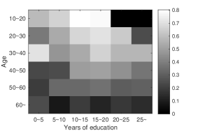
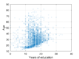
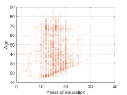
In this section, we carry out simulations on a real-world dataset to evaluate the performance of the proposed algorithms. We use the data collected in [8] which aims to reveal the underlying link between the demand for mobile applications and the user context including age, gender, occupation, years of education, device type (e.g. phone, tablet, and laptop), and nationality. It collects the context information of a total of 10,208 end users and the users’ demand for 23 types of mobile applications. We envision that these mobile applications can be deployed on edge servers at SBSs via containerization and the UEs can send computing tasks to SBS for processing. In our simulation, we consider that the ASP aims to provide edge service for Game-type application (the most popular application out of 23 mobile applications investigated in [8]), which is also a major use case of edge computing. Fig. 5(a) and Fig 5(b) depict the user distribution, and Fig. 5(c) depicts the context-specific service demand estimation on the two context dimensions Age and Years of education. We see clearly that the users’ demand pattern is very related to the users’ context information. Note that the Age and Years of education information is obtained from the dataset [8] and is used only as an example to illustrate the context-demand relationship. In practice, users may be willing to disclose such information in enterprise or campus internal networks. For the more general scenario, SBSs can use other less sensitive context such as user device information.
Refer to caption
(a) Users with service demand
Refer to caption
(b) Users with no service demand
Refer to caption
(c) Oracle demand estimation
Figure 5: User demand pattern on age and year of education dimension

For the small-cell network, we simulate a 1000m×\times1000m area served by N=10𝑁10N=10 SBSs and one MBS. The SBSs are randomly scattered in this area. An SBS can serve users within the service range 150m, which tends to create coverage overlapping among SBSs. For the analysis of non-overlapping SBSs, we assume that users request edge service only from the nearest SBSs; while, in the overlapping case, a user is allowed to decide its association based on the service availability and channel condition of reachable SBSs. To capture different compositions of user population across different SBSs, we randomly assign one out of three area types (school zone, business area, and public) to each SBS, where users with student occupation context tend to show up in school zones with a higher probability, users with full-time worker tend to show up in business areas, and all types of users show up in public with the same probability. The default value of ASP budget is set as b=3𝑏3b=3. Other key simulation parameters are: channel bandwidth W=20𝑊20W=20MHz, transmission power of user equipment Pmu=10subscriptsuperscript𝑃𝑢𝑚10P^{u}_{m}=10dBm, noise power σ2=1010superscript𝜎2superscript1010\sigma^{2}=10^{-10}W/Hz, CPU frequency at SBSs fn=2.8subscript𝑓𝑛2.8f_{n}=2.8GHz, CPU frequency at the cloud f0=5.6subscript𝑓05.6f_{0}=5.6GHz, Internet backhaul transmission rate vt[10,20]superscript𝑣𝑡1020v^{t}\in[10,20]Mbps, round-trip time h=100100h=100ms.

The proposed algorithm is compared with the following benchmarks:
(1) Oracle algorithm: Oracle knows precisely the expected demand for any user context. In each time slot, Oracle selects b𝑏b SBSs that maximize the expected system utility as in (4) based on the observed user context.
(2) Combinatorial UCB (cUCB)[44]: cUCB is developed based on a classic MAB algorithm, UCB1. The key idea is to create super-arms, i.e., b𝑏b-element combination of N𝑁N SBS (b𝑏b is the budget). There will be a total of (Nb)binomial𝑁𝑏N\choose b super-arms and cUCB learns the reward of each super-arm.
(3) Combinatorial-Contextual UCB (c2UCB): c2UCB considers users’ context when running cUCB. Specifically, c2UCB maintains a context space for each super-arm and the utility estimations of hypercubes in a context space are updated when corresponding super-arm is selected.
(4) ϵitalic-ϵ\epsilon-Greedy: ϵitalic-ϵ\epsilon-Greedy rents a random set of b𝑏b SBSs with probability ϵ(0,1)italic-ϵ01\epsilon\in(0,1). With probability (1ϵ)1italic-ϵ(1-\epsilon), the algorithm selects b𝑏b SBSs with highest estimated demands. These estimated demands are calculated based on the previously observed demand of rented SBSs.
(5) Random algorithm: The algorithm simply rents b𝑏b SBSs randomly in each time slot.

VI-A Performance Comparison

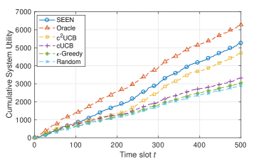
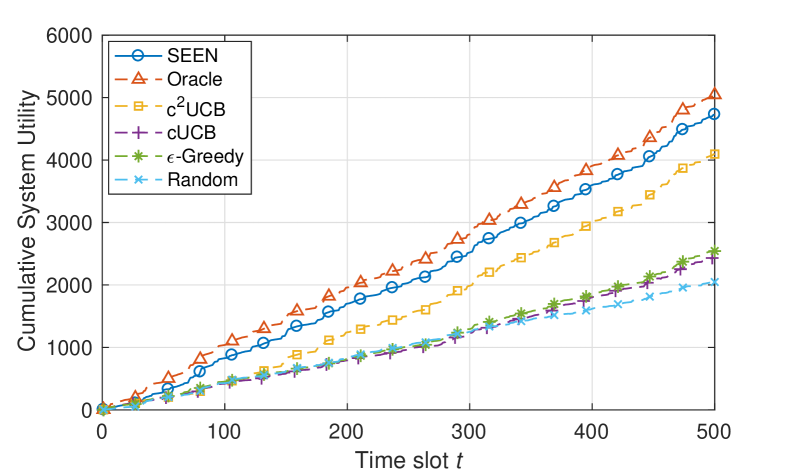
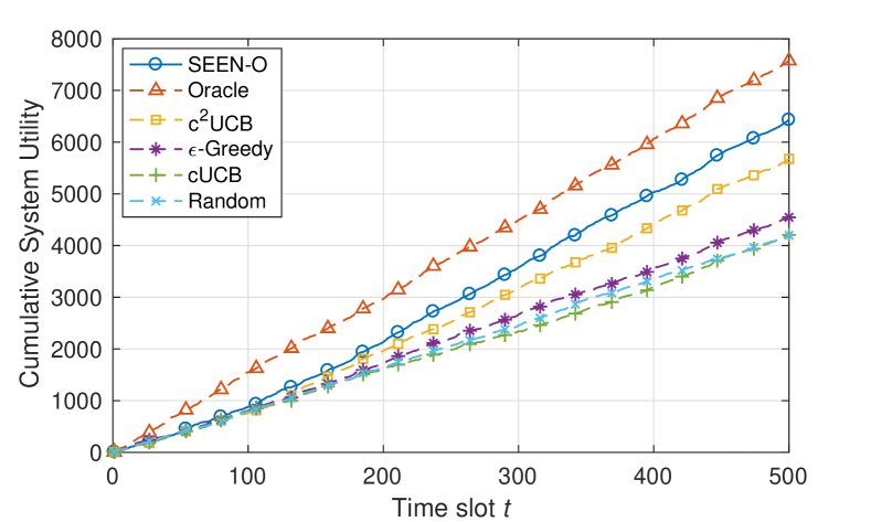
Fig. 7 shows the cumulative system utility achieved by SEEN and other 5 benchmarks for a non-overlapping case. As expected, the Oracle algorithm has the highest cumulative system utility and gives an upper bound to the other algorithms. Among the other algorithms, we see that SEEN and c2UCB significantly outperform cUCB, ϵitalic-ϵ\epsilon-Greedy, and Random algorithm, since they take into account the context information when estimating the users’ service demand pattern. Moreover, SEEN achieves a higher system utility compared with c2UCB. This is due to the fact that c2UCB creates a large set of super-arms and therefore is more likely to enter the exploration phase. The conventional algorithms, cUCB, and ϵitalic-ϵ\epsilon-Greedy, only provide slight improvements compared to the Random algorithm. The failure of these methods is due to the uncertainty of user population in various aspects, e.g. user numbers and composition, which are difficult to estimate in each time slot without observing the user context information.
Refer to caption
Figure 6: Comparison on cumulative system utility.
Refer to caption
Figure 7: MSE of estimated service demand

VI-B Demand estimation error

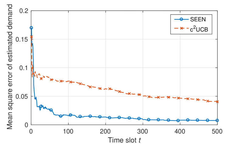
Fig. 7 shows the mean square error (MSE) of service demand estimation achieved by SEEN and c2UCB, where the MSE is measured across all context hypercubes compared to the oracle demand estimation. It can be observed that the MSE of SEEN converges quickly to 0.01 after first 120 time slots while the MSE of c2UCB stays high and decreases slowly during 500-slot runtime. This means that SEEN is able to learn the user demand pattern fast and provide more effective decisions on edge service placement.

VI-C Demand allocation

Fig. 8 shows the allocation of user demand in the network, i.e., whether the demand is processed at the edge or cloud. Note that ASP desires to process more demand at the edge so that lower delay costs are incurred to users. We can see from Fig. 8 that SEEN is able to accommodate a large amount of user demand 62.2%, which is slightly lower than that of Oracle (69.2%). For other four schemes, they rely heavily on the cloud server, therefore incurring large delay cost and diminishing the system utility.
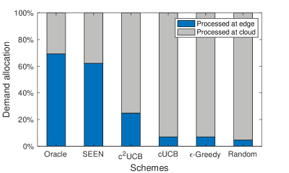
Refer to caption
Figure 8: User demand allocation

VI-D Learning with More Context

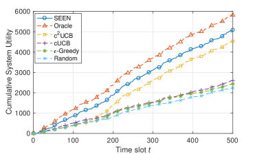
Next, we evaluate the performance of SEEN under different context spaces. Figure 9 shows the cumulative system utilities achieved by SEEN and 5 other benchmarks when running with 2, 3, 4 contexts. Comparing these three figures, we see that the cumulative system utilities achieved by cUCB, ϵitalic-ϵ\epsilon-Greedy, and Random stay more or less the same, since these algorithms are independent of the context information. The context-aware algorithms, i.e., SEEN, Oracle, and c2UCB, achieve higher cumulative utilities with more context information since more contexts help the ASP to learn the users’ demand pattern and therefore make better service provisioning decision. In addition, it is worth noticing that SEEN incurs larger regrets when running with more context information, which is consistent with the analysis in Theorem 1.
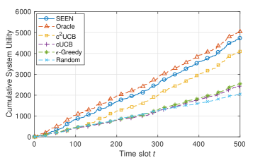
Refer to caption
(a) age, employment status
Refer to caption
(b) age, employment status, marital status
Refer to caption
(c) age, download purpose, employment and marital status
Figure 9: Learning with different context spaces. (a) two-dimension (b) three-dimension (c) four-dimension

VI-E Impact of ASP budget

Fig. 11 depicts the cumulative system utility achieved by 6 schemes in 500 slots with different budgets. As expected, the system utility grows with the increase in ASP budget b𝑏b since more user demand can be processed at the network edge with more SBSs providing edge services. Moreover, we see that SEEN is able to achieve close-to-oracle performance at all levels of ASP budget. By contrast, the c2UCB algorithm suffers an obvious performance degradation with b[4,6]𝑏46b\in[4,6]. This is due to the fact that number of super-arms (Nb)binomial𝑁𝑏N\choose b created by c2UCB becomes very large given N=10𝑁10N=10 and b[4,6]𝑏46b\in[4,6]. This forces the c2UCB algorithm to enter exploration more frequently and leads to system utility loss.
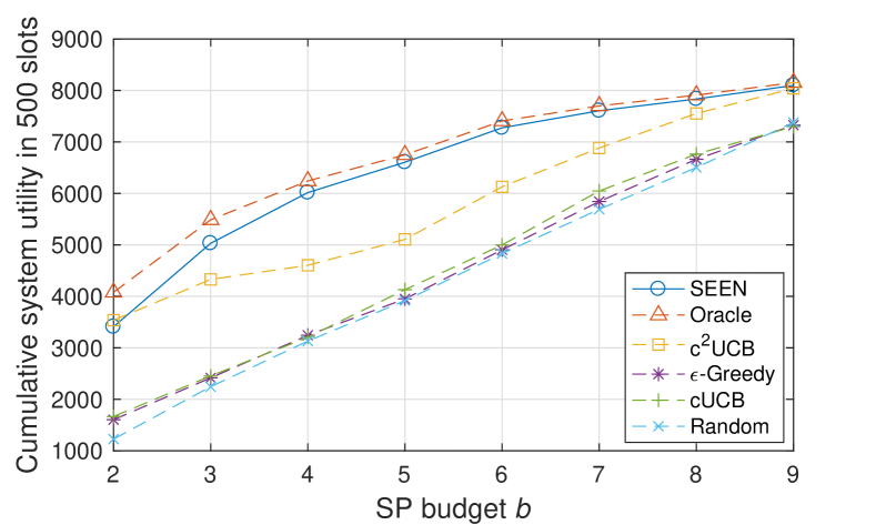
Refer to caption
Figure 10: Impact of ASP budget.
Refer to caption
Figure 11: Comparison on cumulative utility (overlapped coverage).

VI-F Edge Service Placement with Overlapping Coverage

Fig. 11 compares the performance achieved by SEEN-O and 5 other benchmarks when applied to the overlapping case. Similar to the non-overlapping case, we see that the context-aware schemes far outperform conventional MAB algorithms and SEEN-O achieves the highest cumulative system utility except for Oracle. However, it can be observed that SEEN-O incurs a larger regret compared to the non-overlapping case. This is because users in the overlapped area are observed by multiple SBSs and their contexts are duplicated when determining the under-explored SBSs. This increases the probability of being under-explored for SBSs and pushes SEEN-O to enter the exploration phase. Nevertheless, it does not mean that considering coverage overlapping leads to the performance degradation. SEEN-O actually achieves a higher cumulative system utility compared to that of SEEN achieved in the non-overlapping case.

VI-G Impact of Overlapping Degree

The overlapping degree of the edge network is defined as Sco-cover/Stotalsubscript𝑆co-coversubscript𝑆totalS_{\text{co-cover}}/S_{\text{total}} where Sco-coversubscript𝑆co-coverS_{\text{co-cover}} is the service area co-covered by at least two SBSs and Stotalsubscript𝑆totalS_{\text{total}} is the total service area. In the following, we show the impact of overlapping degree on the performance of SEEN. Fig. 12 depicts the cumulative system utilities achieved by SEEN-O and Random in 500 time slots with different overlapping degrees. It also shows the cumulative system utility achieved by SEEN in the non-overlapping case for comparison. In general, we see that a larger overlapping degree results in higher system utilities for both SEEN-O and Random. This is because more users can access multiple SBSs for edge service given a larger overlapping degree, and therefore the ASP can further optimize the edge service placement decisions to accommodate more service demand at the Internet edge by exploiting the flexible association of users. By comparing SEEN-O and SEEN, we also see that considering the SBS coverage overlapping helps improve the system utility and the improvement grows with the increase in the overlapping degree.
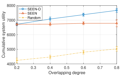
Refer to caption
Figure 12: Impact of overlapping degree

VII Conclusion

In this paper, we investigated the edge service placement problem of an ASP in radio access networks integrated with shared edge computing platforms. To cope with the unknown and fluctuating service demand among changing user populations, we formulated a novel combinatorial contextual bandit learning problem and proposed an efficient learning algorithm to make optimal spatial-temporal dynamic edge service placement decisions. The proposed algorithm is practical, easy to implement and scalable to large networks while achieving provably asymptotically optimal performance. However, there are still efforts need to be done to improve the existing CC-MAB framework. First, we currently use a simple static partition of context space. Considering dynamic partition may further help improve the algorithm performance by generating more appropriate hypercubes. Second, our paper only provides a regret upper bound for SEEN. A meaningful complementary is to analyze the regret lower bound. Besides the investigated edge service placement problem, CC-MAB can also be applied to many other sequential decision making problems under uncertainty that involve multiple-play given a limited budget and context.

References

  • [1] A. Li, X. Yang, S. Kandula, and M. Zhang, “Cloudcmp: comparing public cloud providers,” in Proceedings of the 10th ACM SIGCOMM conference on Internet measurement.   ACM, 2010, pp. 1–14.
  • [2] T. Taleb, S. Dutta, A. Ksentini, M. Iqbal, and H. Flinck, “Mobile edge computing potential in making cities smarter,” IEEE Communications Magazine, vol. 55, no. 3, pp. 38–43, March 2017.
  • [3] Vapor IO, https://www.vapor.io/.
  • [4] Project Volutus, https://www.vapor.io/project-volutus-extending-the-cloud-to-the-true-edge/.
  • [5] Intel, “Smart cells revolutionize service delivery,” https://www.intel.com/content/dam/www/public/us/en/documents/white-papers/smart-cells-revolutionize-service-delivery.pdf.
  • [6] M. STANSBERRY, “Uptime institute-data center industry survey 2013.”
  • [7] T. L. Lai and H. Robbins, “Asymptotically efficient adaptive allocation rules,” Advances in applied mathematics, vol. 6, no. 1, pp. 4–22, 1985.
  • [8] S. L. Lim, P. J. Bentley, N. Kanakam, F. Ishikawa, and S. Honiden, “Investigating country differences in mobile app user behavior and challenges for software engineering,” IEEE Transactions on Software Engineering, vol. 41, no. 1, pp. 40–64, 2015.
  • [9] Y. Mao, C. You, J. Zhang, K. Huang, and K. B. Letaief, “A survey on mobile edge computing: The communication perspective,” IEEE Communications Surveys & Tutorials, 2017.
  • [10] W. Shi, J. Cao, Q. Zhang, Y. Li, and L. Xu, “Edge computing: Vision and challenges,” IEEE Internet of Things Journal, vol. 3, no. 5, pp. 637–646, 2016.
  • [11] D. Huang, P. Wang, and D. Niyato, “A dynamic offloading algorithm for mobile computing,” IEEE Trans. on Wireless Communications, vol. 11, no. 6, pp. 1991–1995, 2012.
  • [12] J. Liu, Y. Mao, J. Zhang, and K. B. Letaief, “Delay-optimal computation task scheduling for mobile-edge computing systems,” in Information Theory (ISIT), 2016 IEEE International Symposium on.   IEEE, 2016, pp. 1451–1455.
  • [13] J. Xu, L. Chen, and S. Ren, “Online learning for offloading and autoscaling in energy harvesting mobile edge computing,” IEEE Trans. on Cognitive Communications and Networking, vol. PP, no. P, pp. 1–15, 2017.
  • [14] Y. Mao, J. Zhang, and K. B. Letaief, “Dynamic computation offloading for mobile-edge computing with energy harvesting devices,” IEEE Journal on Selected Areas in Communications, vol. 34, no. 12, pp. 3590–3605, 2016.
  • [15] L. Chen and J. Xu, “Socially trusted collaborative edge computing in ultra dense networks,” in Proceedings of the Second ACM/IEEE Symposium on Edge Computing.   ACM, 2017, p. 9.
  • [16] S. Tanzil, O. Gharehshiran, and V. Krishnamurthy, “A distributed coalition game approach to femto-cloud formation,” IEEE Trans. on Cloud Computing, 2016.
  • [17] Y. Chen, R. H. Katz, and J. D. Kubiatowicz, “Dynamic replica placement for scalable content delivery,” in International Workshop on Peer-to-Peer Systems.   Springer, 2002, pp. 306–318.
  • [18] K. Shanmugam, N. Golrezaei, A. G. Dimakis, A. F. Molisch, and G. Caire, “Femtocaching: Wireless content delivery through distributed caching helpers,” IEEE Transactions on Information Theory, vol. 59, no. 12, pp. 8402–8413, 2013.
  • [19] Q. Zhang, Q. Zhu, M. F. Zhani, R. Boutaba, and J. L. Hellerstein, “Dynamic service placement in geographically distributed clouds,” IEEE Journal on Selected Areas in Communications, vol. 31, no. 12, pp. 762–772, 2013.
  • [20] J. Xu, L. Chen, and P. Zhou, “Joint service caching and task offloading for mobile edge computing in dense networks,” in International Conference on Computer Communications(INFOCOM).   IEEE, 2018, pp. 1–9.
  • [21] L. Chen and J. Xu, “Collaborative service caching for edge computing in dense small cell networks,” arXiv preprint arXiv:1709.08662, 2017.
  • [22] S. Müller, O. Atan, M. van der Schaar, and A. Klein, “Context-aware proactive content caching with service differentiation in wireless networks,” IEEE Transactions on Wireless Communications, vol. 16, no. 2, pp. 1024–1036, 2017.
  • [23] P. Auer, N. Cesa-Bianchi, and P. Fischer, “Finite-time analysis of the multiarmed bandit problem,” Machine learning, vol. 47, no. 2-3, pp. 235–256, 2002.
  • [24] R. Agrawal, “Sample mean based index policies by o(logn)𝑜𝑛o(\log n) regret for the multi-armed bandit problem,” Advances in Applied Probability, vol. 27, no. 4, pp. 1054–1078, 1995.
  • [25] V. Anantharam, P. Varaiya, and J. Walrand, “Asymptotically efficient allocation rules for the multiarmed bandit problem with multiple plays-part i: Iid rewards,” IEEE Transactions on Automatic Control, vol. 32, no. 11, pp. 968–976, 1987.
  • [26] R. Agrawal, M. Hegde, and D. Teneketzis, “Multi-armed bandit problems with multiple plays and switching cost,” Stochastics and Stochastic reports, vol. 29, no. 4, pp. 437–459, 1990.
  • [27] Y. Gai, B. Krishnamachari, and R. Jain, “Combinatorial network optimization with unknown variables: Multi-armed bandits with linear rewards and individual observations,” IEEE/ACM Transactions on Networking (TON), vol. 20, no. 5, pp. 1466–1478, 2012.
  • [28] A. Slivkins, “Contextual bandits with similarity information,” in Proceedings of the 24th annual Conference On Learning Theory, 2011, pp. 679–702.
  • [29] L. Li, W. Chu, J. Langford, and R. E. Schapire, “A contextual-bandit approach to personalized news article recommendation,” in Proceedings of the 19th international conference on World wide web.   ACM, 2010, pp. 661–670.
  • [30] C. Tekin and M. van der Schaar, “Distributed online learning via cooperative contextual bandits,” IEEE Transactions on Signal Processing, vol. 63, no. 14, pp. 3700–3714, 2015.
  • [31] L. Qin, S. Chen, and X. Zhu, “Contextual combinatorial bandit and its application on diversified online recommendation,” in Proceedings of the 2014 SIAM International Conference on Data Mining.   SIAM, 2014, pp. 461–469.
  • [32] S. Li, B. Wang, S. Zhang, and W. Chen, “Contextual combinatorial cascading bandits,” in International Conference on Machine Learning, 2016, pp. 1245–1253.
  • [33] C. Pahl, “Containerization and the paas cloud,” IEEE Cloud Computing, vol. 2, no. 3, pp. 24–31, 2015.
  • [34] D. Bernstein, “Containers and cloud: From lxc to docker to kubernetes,” IEEE Cloud Computing, vol. 1, no. 3, pp. 81–84, 2014.
  • [35] B. Russell, “Kvm and docker lxc benchmarking with openstack,” 2014.
  • [36] Q. Fan and N. Ansari, “Workload allocation in hierarchical cloudlet networks,” IEEE Communications Letters, vol. 22, no. 4, pp. 820–823, 2018.
  • [37] S. Lederer, J. Mankoff, A. K. Dey, and C. Beckmann, “Managing personal information disclosure in ubiquitous computing environments,” Intel Research, IRB-TR-03-015, 2003.
  • [38] D. Anthony, T. Henderson, and D. Kotz, “Privacy in location-aware computing environments,” IEEE Pervasive Computing, vol. 6, no. 4, 2007.
  • [39] I. Bilogrevic, K. Huguenin, B. Agir, M. Jadliwala, M. Gazaki, and J.-P. Hubaux, “A machine-learning based approach to privacy-aware information-sharing in mobile social networks,” Pervasive and Mobile Computing, vol. 25, pp. 125–142, 2016.
  • [40] Online appendix: Spatio-temporal edge service placement: A bandit learning approach. [Online]. Available: https://www.dropbox.com/sh/hrzv46x78yjy3fl/AAAQ6YCjPcg8PvYIExjgwoyJa?dl=0
  • [41] T. Yamada, S. Kataoka, and K. Watanabe, “Heuristic and exact algorithms for the disjunctively constrained knapsack problem,” Information Processing Society of Japan Journal, vol. 43, no. 9, 2002.
  • [42] M. Hifi and N. Otmani, “An algorithm for the disjunctively constrained knapsack problem,” International Journal of Operational Research, vol. 13, no. 1, pp. 22–43, 2012.
  • [43] A. Bettinelli, V. Cacchiani, and E. Malaguti, “A branch-and-bound algorithm for the knapsack problem with conflict graph,” INFORMS Journal on Computing, vol. 29, no. 3, pp. 457–473, 2017.
  • [44] W. Chen, Y. Wang, and Y. Yuan, “Combinatorial multi-armed bandit: General framework and applications,” in International Conference on Machine Learning, 2013, pp. 151–159.
  • [45] W. Hoeffding, “Probability inequalities for sums of bounded random variables,” Journal of the American statistical association, vol. 58, no. 301, pp. 13–30, 1963.

Appendix A Proof of Theorem 1

The regret bound of SEEN is derived based on the natural assumption that the expected demands of users are similar if they have similar context as captured by the the Hölder condition. The Hölder condition allows us to derive a regret bound, which shows that the regret of SEEN is sublinear in the time horizon T𝑇T, i.e. R(T)=O(Tγ)𝑅𝑇𝑂superscript𝑇𝛾R(T)=O(T^{\gamma}) with γ<1𝛾1\gamma<1.

For each SBS n𝒩𝑛𝒩n\in\mathcal{N} and each hypercube p𝒫n,T,n𝑝subscript𝒫𝑛𝑇for-all𝑛p\in\mathcal{P}_{n,T},\forall n, we define μ¯(p)=supxpμ(x)¯𝜇𝑝subscriptsupremum𝑥𝑝𝜇𝑥\bar{\mu}(p)=\sup_{x\in p}\mu(x) and μ¯(p)=infxpμ(x)¯𝜇𝑝subscriptinfimum𝑥𝑝𝜇𝑥\underaccent{\bar}{\mu}(p)=\inf_{x\in p}\mu(x) be the best and worst expected demand over all contexts x𝑥x from hypercube p𝑝p respectively. In some steps of the proofs, we have to compare the demands at different positions in a hypercube. As a point of reference, we define the context at the (geometrical) center of a hypercube p𝑝p as x(p)superscript𝑥𝑝x^{*}(p). Also, we define the top-b𝑏b SBSs for hypercubes in 𝑷tsuperscript𝑷𝑡{\boldsymbol{P}}^{t} as following b𝑏b SBSs 𝒮t(𝑷t)={n1(𝑷t),,nb(𝑷t)}superscript𝒮absent𝑡superscript𝑷𝑡subscriptsuperscript𝑛1superscript𝑷𝑡subscriptsuperscript𝑛𝑏superscript𝑷𝑡\mathcal{S}^{*t}({\boldsymbol{P}}^{t})=\{n^{*}_{1}({\boldsymbol{P}}^{t}),\dots,n^{*}_{b}({\boldsymbol{P}}^{t})\} which satisfy

n1(𝑷t)argmaxn𝒩mntu~n,mμ(x(pn,mt))subscriptsuperscript𝑛1superscript𝑷𝑡subscriptargmax𝑛𝒩subscript𝑚subscriptsuperscript𝑡𝑛subscript~𝑢𝑛𝑚𝜇superscript𝑥subscriptsuperscript𝑝𝑡𝑛𝑚\displaystyle n^{*}_{1}({\boldsymbol{P}}^{t})\in\operatorname*{arg\,max}_{n\in\mathcal{N}}\sum_{m\in\mathcal{M}^{t}_{n}}\tilde{u}_{n,m}\mu(x^{*}(p^{t}_{n,m}))
n2(𝑷t)argmaxn𝒩\{n1(𝑷t)}mntu~n,mμ(x(pn,mt))subscriptsuperscript𝑛2superscript𝑷𝑡subscriptargmax𝑛\𝒩subscriptsuperscript𝑛1superscript𝑷𝑡subscript𝑚subscriptsuperscript𝑡𝑛subscript~𝑢𝑛𝑚𝜇superscript𝑥subscriptsuperscript𝑝𝑡𝑛𝑚\displaystyle n^{*}_{2}({\boldsymbol{P}}^{t})\in\operatorname*{arg\,max}_{n\in\mathcal{N}\backslash\{n^{*}_{1}({\boldsymbol{P}}^{t})\}}\sum_{m\in\mathcal{M}^{t}_{n}}\tilde{u}_{n,m}\mu(x^{*}(p^{t}_{n,m}))
\displaystyle\qquad\vdots
nb(𝑷t)argmaxn𝒩\{n1(𝑷t),,nb1(𝑷t)}mntu~n,mμ(x(pn,mt))subscriptsuperscript𝑛𝑏superscript𝑷𝑡subscriptargmax𝑛\𝒩subscriptsuperscript𝑛1superscript𝑷𝑡subscriptsuperscript𝑛𝑏1superscript𝑷𝑡subscript𝑚subscriptsuperscript𝑡𝑛subscript~𝑢𝑛𝑚𝜇superscript𝑥subscriptsuperscript𝑝𝑡𝑛𝑚\displaystyle n^{*}_{b}({\boldsymbol{P}}^{t})\in\operatorname*{arg\,max}_{n\in\mathcal{N}\backslash\{n^{*}_{1}({\boldsymbol{P}}^{t}),\dots,n^{*}_{b-1}({\boldsymbol{P}}^{t})\}}\sum_{m\in\mathcal{M}^{t}_{n}}\tilde{u}_{n,m}\mu(x^{*}(p^{t}_{n,m}))

𝒮t(𝑷t)superscript𝒮absent𝑡superscript𝑷𝑡\mathcal{S}^{*t}({\boldsymbol{P}}^{t}) can be used to identify subsets of SBSs which are bad choices to rent when its users’ contexts are from hypercubes 𝒑nt=(pn,mt)mntsubscriptsuperscript𝒑𝑡𝑛subscriptsubscriptsuperscript𝑝𝑡𝑛𝑚𝑚subscriptsuperscript𝑡𝑛{\boldsymbol{p}}^{t}_{n}=(p^{t}_{n,m})_{m\in\mathcal{M}^{t}_{n}}. Let

t(𝑷t)={G={n1,,nb}𝒩,|G|=b:\displaystyle\mathcal{L}^{t}({\boldsymbol{P}}^{t})=\big{\{}G=\{n_{1},\dots,n_{b}\}\subseteq\mathcal{N},|G|=b:
nS,tmntu~n,mμ¯(pn,mt)nGmntu~n,mμ¯(pn,mt)Atθ}\displaystyle\sum_{n\in S^{*,t}}\sum_{m\in\mathcal{M}^{t}_{n}}\tilde{u}_{n,m}\underaccent{\bar}{\mu}(p^{t}_{n,m})-\sum_{n\in G}\sum_{m\in\mathcal{M}^{t}_{n}}\tilde{u}_{n,m}\bar{\mu}(p^{t}_{n,m})\geq At^{\theta}\big{\}} (18)

be the set of suboptimal subsets of SBSs for the users’ context 𝑷tsuperscript𝑷𝑡{\boldsymbol{P}}^{t}, where A>0𝐴0A>0 and θ<0𝜃0\theta<0 are parameters used only in the regret analysis. We call a subset G𝐺G of SBSs in t(𝑷t)superscript𝑡superscript𝑷𝑡\mathcal{L}^{t}({\boldsymbol{P}}^{t}) suboptimal for 𝑷tsuperscript𝑷𝑡{\boldsymbol{P}}^{t}, since the sum of the worst expected demands for 𝒮t(𝑷t)superscript𝒮absent𝑡superscript𝑷𝑡\mathcal{S}^{*t}({\boldsymbol{P}}^{t}) is at least an amount Atθ𝐴superscript𝑡𝜃At^{\theta} higher than the sum of the best expected demands for subset G𝐺G. We call subsets in 𝒩b\t(𝑷t)\subscript𝒩𝑏superscript𝑡superscript𝑷𝑡\mathcal{N}_{b}\backslash\mathcal{L}^{t}({\boldsymbol{P}}^{t}) near-optimal for 𝑷tsuperscript𝑷𝑡{\boldsymbol{P}}^{t}. Here, 𝒩bsubscript𝒩𝑏\mathcal{N}_{b} denotes the set of all b𝑏b-element subsets of set 𝒩𝒩\mathcal{N}. Then the regret R(T)𝑅𝑇R(T) can be divided into the following three summands

R(T)=𝔼[Re(T)]+𝔼[Rs(T)]+𝔼[Rn(T)]𝑅𝑇𝔼delimited-[]subscript𝑅𝑒𝑇𝔼delimited-[]subscript𝑅𝑠𝑇𝔼delimited-[]subscript𝑅𝑛𝑇\displaystyle R(T)=\mathbb{E}[R_{e}(T)]+\mathbb{E}[R_{s}(T)]+\mathbb{E}[R_{n}(T)] (19)

where the term 𝔼[Re(T)]𝔼delimited-[]subscript𝑅𝑒𝑇\mathbb{E}[R_{e}(T)] is the regret due to exploration phases and the term 𝔼[Rs(T)]𝔼delimited-[]subscript𝑅𝑠𝑇\mathbb{E}[R_{s}(T)] and 𝔼[Rn(T)]𝔼delimited-[]subscript𝑅𝑛𝑇\mathbb{E}[R_{n}(T)] are regrets in exploitation phases: the term 𝔼[Rs(T)]𝔼delimited-[]subscript𝑅𝑠𝑇\mathbb{E}[R_{s}(T)] is the regret due to suboptimal choices, i.e., when subsets of SBSs from t(𝑷t)superscript𝑡superscript𝑷𝑡\mathcal{L}^{t}({\boldsymbol{P}}^{t}) are rented; the term 𝔼[Rn(T)]𝔼delimited-[]subscript𝑅𝑛𝑇\mathbb{E}[R_{n}(T)] is the regret due to near-optimal choices, i.e., when subsets of SBSs from 𝒩b\t(𝑷t)\subscript𝒩𝑏superscript𝑡superscript𝑷𝑡\mathcal{N}_{b}\backslash\mathcal{L}^{t}({\boldsymbol{P}}^{t}) are rented. Later, we will show that each of the three summands is bounded.

We first give the bound of 𝔼[Re(T)]𝔼delimited-[]subscript𝑅𝑒𝑇\mathbb{E}[R_{e}(T)] as shown in Lemma 1.

Lemma 1 (Bound for 𝔼(Re(T))𝔼subscript𝑅𝑒𝑇\mathbb{E}(R_{e}(T))).

Let Kn(t)=tznlog(t)subscript𝐾𝑛𝑡superscript𝑡subscript𝑧𝑛𝑡K_{n}(t)=t^{z_{n}}\log(t) and hn,T=Tγnsubscript𝑛𝑇superscript𝑇subscript𝛾𝑛h_{n,T}=\lceil T^{\gamma_{n}}\rceil, where 0<zn<10subscript𝑧𝑛10<z_{n}<1 and 0<γn<1Dn0subscript𝛾𝑛1subscript𝐷𝑛0<\gamma_{n}<\frac{1}{D_{n}}. If SEEN is run with these parameters, the regret 𝔼[Re(T)]𝔼delimited-[]subscript𝑅𝑒𝑇\mathbb{E}[R_{e}(T)] is bounded by

𝔼[Re(T)]bu~maxMmaxdmaxn𝒩2Dn(log(T)Tzn+γnDn+TγnDn)𝔼delimited-[]subscript𝑅𝑒𝑇𝑏superscript~𝑢superscript𝑀superscript𝑑subscript𝑛𝒩superscript2subscript𝐷𝑛𝑇superscript𝑇subscript𝑧𝑛subscript𝛾𝑛subscript𝐷𝑛superscript𝑇subscript𝛾𝑛subscript𝐷𝑛\displaystyle\mathbb{E}[R_{e}(T)]\leq b\tilde{u}^{\max}M^{\max}d^{\max}\sum_{n\in\mathcal{N}}2^{D_{n}}\left(\log(T)T^{z_{n}+\gamma_{n}D_{n}}+T^{\gamma_{n}D_{n}}\right) (20)
Proof of Lemma 1.

Let t𝑡t be an exploration phase, then by the definition of SEEN, the set of under-explored SBSs 𝒩ue,tsuperscript𝒩ue𝑡\mathcal{N}^{\text{ue},t} is non-empty in exploration, i.e., there exist a SBS n𝑛n and a hypercube pn,mt,mntsubscriptsuperscript𝑝𝑡𝑛𝑚𝑚subscriptsuperscript𝑡𝑛p^{t}_{n,m},m\in\mathcal{M}^{t}_{n} with Cnt(pn,mt)Kn(t)=tznlog(t)subscriptsuperscript𝐶𝑡𝑛subscriptsuperscript𝑝𝑡𝑛𝑚subscript𝐾𝑛𝑡superscript𝑡subscript𝑧𝑛𝑡C^{t}_{n}(p^{t}_{n,m})\leq K_{n}(t)=t^{z_{n}}\log(t). Clearly, there can be at most Tznlog(T)superscript𝑇subscript𝑧𝑛𝑇\lceil T^{z_{n}}\log(T)\rceil exploration phases in which SBS n𝑛n is rented due to its under-exploration. Since there are (hn,T)Dnsuperscriptsubscript𝑛𝑇subscript𝐷𝑛(h_{n,T})^{D_{n}} hypercubes in the partition, there can be at most (hn,T)DnTznlog(T)superscriptsubscript𝑛𝑇subscript𝐷𝑛superscript𝑇subscript𝑧𝑛𝑇(h_{n,T})^{D_{n}}\lceil T^{z_{n}}\log(T)\rceil exploration phases in which SBS n𝑛n is rent due to its under-exploration. In each of these exploration phase, the maximum loss in demand due to wrong selection of a user in SBS n𝑛n is bounded by Δmax:=maxx𝒳n,x𝒳n|μ(x)μ(x)|assignsuperscriptΔsubscriptformulae-sequence𝑥subscript𝒳𝑛superscript𝑥subscript𝒳superscript𝑛𝜇𝑥𝜇superscript𝑥\Delta^{\max}:=\max_{x\in\mathcal{X}_{n},x^{\prime}\in\mathcal{X}_{n^{\prime}}}|\mu(x)-\mu(x^{\prime})|. Notice the random demand μ(x)𝜇𝑥\mu(x) for any x𝒳n,n𝒩formulae-sequence𝑥subscript𝒳𝑛𝑛𝒩x\in\mathcal{X}_{n},n\in\mathcal{N}, is bounded in [0,dmax]0superscript𝑑[0,d^{\max}], it holds that ΔmaxdmaxsuperscriptΔsuperscript𝑑\Delta^{\max}\leq d^{\max}. Let u~maxsuperscript~𝑢\tilde{u}^{\max} be the maximum achievable delay improvement for any SBS n𝑛n by completing a unit workload (a task) for user mnt𝑚subscriptsuperscript𝑡𝑛m\in\mathcal{M}^{t}_{n}. Since the maximum number of users can be served by an SBS per time slot is Mmaxsuperscript𝑀M^{\max}, the maximum loss for wrong selection of SBS n𝑛n is bounded by u~maxMmaxdmaxsuperscript~𝑢superscript𝑀superscript𝑑\tilde{u}^{\max}M^{\max}d^{\max}. Additionally, we have to take into account the loss due to exploitations in the case that the size of under-explored SBSs is smaller than b𝑏b. In each of the exploration phases in which SBS n𝑛n is selected, if the size of 𝒩ue,tsuperscript𝒩ue𝑡\mathcal{N}^{\text{ue},t} is smaller than b𝑏b, the maximum additional loss is (b1)u~maxMmaxdmax𝑏1superscript~𝑢superscript𝑀superscript𝑑(b-1)\tilde{u}^{\max}M^{\max}d^{\max}. Therefore, in each of exploration phase in which n𝑛n is selected, the overall maximum loss due to wrong selection of SBS n𝑛n is bu~maxMmaxdmax𝑏superscript~𝑢superscript𝑀superscript𝑑b\tilde{u}^{\max}M^{\max}d^{\max}. Summing over all n𝒩𝑛𝒩n\in\mathcal{N} yields:

𝔼[Re(T)]𝔼delimited-[]subscript𝑅𝑒𝑇\displaystyle\mathbb{E}[R_{e}(T)] bu~maxMmaxdmaxn𝒩(hn,T)DnTznlog(T)absent𝑏superscript~𝑢superscript𝑀superscript𝑑subscript𝑛𝒩superscriptsubscript𝑛𝑇subscript𝐷𝑛superscript𝑇subscript𝑧𝑛𝑇\displaystyle\leq b\tilde{u}^{\max}M^{\max}d^{\max}\sum_{n\in\mathcal{N}}(h_{n,T})^{D_{n}}\lceil T^{z_{n}}\log(T)\rceil (21)
=bu~maxMmaxdmaxn𝒩(Tγn)DnTznlog(T)absent𝑏superscript~𝑢superscript𝑀superscript𝑑subscript𝑛𝒩superscriptsuperscript𝑇subscript𝛾𝑛subscript𝐷𝑛superscript𝑇subscript𝑧𝑛𝑇\displaystyle=b\tilde{u}^{\max}M^{\max}d^{\max}\sum_{n\in\mathcal{N}}(T^{\gamma_{n}})^{D_{n}}\lceil T^{z_{n}}\log(T)\rceil (22)

Using TγnDn(2Tγn)Dn=2DnTγnDnsuperscriptsuperscript𝑇subscript𝛾𝑛subscript𝐷𝑛superscript2superscript𝑇subscript𝛾𝑛subscript𝐷𝑛superscript2subscript𝐷𝑛superscript𝑇subscript𝛾𝑛subscript𝐷𝑛\lceil T^{\gamma_{n}}\rceil^{D_{n}}\leq(2T^{\gamma_{n}})^{D_{n}}=2^{D_{n}}T^{\gamma_{n}D_{n}}, it holds

𝔼[Re(T)]bu~maxMmaxdmaxn𝒩2Dn(log(T)Tzn+γnDn+TγnDn)𝔼delimited-[]subscript𝑅𝑒𝑇𝑏superscript~𝑢superscript𝑀superscript𝑑subscript𝑛𝒩superscript2subscript𝐷𝑛𝑇superscript𝑇subscript𝑧𝑛subscript𝛾𝑛subscript𝐷𝑛superscript𝑇subscript𝛾𝑛subscript𝐷𝑛\displaystyle\mathbb{E}[R_{e}(T)]\leq b\tilde{u}^{\max}M^{\max}d^{\max}\sum_{n\in\mathcal{N}}2^{D_{n}}\left(\log(T)T^{z_{n}+\gamma_{n}D_{n}}+T^{\gamma_{n}D_{n}}\right) (23)

Next, we give a bound for 𝔼[Rs(T)]𝔼delimited-[]subscript𝑅𝑠𝑇\mathbb{E}[R_{s}(T)]. This bound also depends on the choice of two parameters znsubscript𝑧𝑛z_{n} and γnsubscript𝛾𝑛\gamma_{n} for each SBS. Additionally, a condition on these parameters has to be satisfied.

Lemma 2 (Bound for 𝔼(Rs(T))𝔼subscript𝑅𝑠𝑇\mathbb{E}(R_{s}(T))).

Let Kn(t)=tznlog(t)subscript𝐾𝑛𝑡superscript𝑡subscript𝑧𝑛𝑡K_{n}(t)=t^{z_{n}}\log(t) and hn,T=Tγnsubscript𝑛𝑇superscript𝑇subscript𝛾𝑛h_{n,T}=\lceil T^{\gamma_{n}}\rceil, where 0<zn<10subscript𝑧𝑛10<z_{n}<1 and 0<γn<1Dn0subscript𝛾𝑛1subscript𝐷𝑛0<\gamma_{n}<\frac{1}{D_{n}}. If SEEN is run with these parameters, Assumption 1 holds true and the additional condition 2H(t)+u~maxMmax(nGLnDnαn2hn,Tαn+n𝒮t(𝐏t)LnDnαn2hn,Tαn)Atθ2𝐻𝑡superscript~𝑢superscript𝑀subscript𝑛𝐺subscript𝐿𝑛superscriptsubscript𝐷𝑛subscript𝛼𝑛2subscriptsuperscriptsubscript𝛼𝑛𝑛𝑇subscript𝑛superscript𝒮absent𝑡superscript𝐏𝑡subscript𝐿𝑛superscriptsubscript𝐷𝑛subscript𝛼𝑛2subscriptsuperscriptsubscript𝛼𝑛𝑛𝑇𝐴superscript𝑡𝜃2H(t)+\tilde{u}^{\max}M^{\max}\left(\sum_{n\in G}L_{n}D_{n}^{\frac{\alpha_{n}}{2}}h^{-\alpha_{n}}_{n,T}+\sum_{n\in\mathcal{S}^{*t}({\boldsymbol{P}}^{t})}L_{n}D_{n}^{\frac{\alpha_{n}}{2}}h^{-\alpha_{n}}_{n,T}\right)\leq At^{\theta} is satisfied for all 1tT1𝑡𝑇1\leq t\leq T where H(t):=bu~maxMmaxdmaxtzmin/2,zmin=minnznformulae-sequenceassign𝐻𝑡𝑏superscript~𝑢superscript𝑀superscript𝑑superscript𝑡superscript𝑧2superscript𝑧subscript𝑛subscript𝑧𝑛H(t):=b\tilde{u}^{\max}M^{\max}d^{\max}t^{-z^{\min}/2},z^{\min}=\min_{n}z_{n}. Then the regret 𝔼[Rs(T)]𝔼delimited-[]subscript𝑅𝑠𝑇\mathbb{E}[R_{s}(T)] is bounded by

𝔼[Rs(T)]b2u~max(Mmax)2dmax(Nb)π23𝔼delimited-[]subscript𝑅𝑠𝑇superscript𝑏2superscript~𝑢superscriptsuperscript𝑀2superscript𝑑binomial𝑁𝑏superscript𝜋23\displaystyle\mathbb{E}[R_{s}(T)]\leq b^{2}\tilde{u}^{\max}(M^{\max})^{2}d^{\max}{N\choose b}\frac{\pi^{2}}{3} (24)
Proof of Lemma 2.

For 1tT1𝑡𝑇1\leq t\leq T, let W(t)={𝒩ue,t=}𝑊𝑡superscript𝒩ue𝑡W(t)=\{\mathcal{N}^{\text{ue},t}=\emptyset\} be the even that slot t𝑡t is an exploitation phase. By the definition of 𝒩ue,tsuperscript𝒩ue𝑡\mathcal{N}^{\text{ue},t}, in this exploitation, it holds that Cnt(pn,mt)>Kn(t)=tznlog(t)subscriptsuperscript𝐶𝑡𝑛subscriptsuperscript𝑝𝑡𝑛𝑚subscript𝐾𝑛𝑡superscript𝑡subscript𝑧𝑛𝑡C^{t}_{n}(p^{t}_{n,m})>K_{n}(t)=t^{z_{n}}\log(t) for all n𝒩𝑛𝒩n\in\mathcal{N} and all mnt𝑚subscriptsuperscript𝑡𝑛m\in\mathcal{M}^{t}_{n}. Let VG(t)subscript𝑉𝐺𝑡V_{G}(t) be the event that subset G𝐺G is rented at time slot t𝑡t. Then, it holds that

Rs(T)=subscript𝑅𝑠𝑇absent\displaystyle R_{s}(T)= t=1TGt(𝑷t)I{VG(t),W(t)}×\displaystyle\sum_{t=1}^{T}\sum_{G\in\mathcal{L}^{t}({\boldsymbol{P}}^{t})}I_{\{V_{G}(t),W(t)\}}\times
(nSt(𝑿t)mntu~n,md(xn,mt)nGmntu~n,md(xn,mt))subscript𝑛superscript𝑆absent𝑡superscript𝑿𝑡subscript𝑚subscriptsuperscript𝑡𝑛subscript~𝑢𝑛𝑚𝑑subscriptsuperscript𝑥𝑡𝑛𝑚subscript𝑛𝐺subscript𝑚subscriptsuperscript𝑡𝑛subscript~𝑢𝑛𝑚𝑑subscriptsuperscript𝑥𝑡𝑛𝑚\displaystyle\left(\sum_{n\in S^{*t}({\boldsymbol{X}}^{t})}\sum_{m\in\mathcal{M}^{t}_{n}}\tilde{u}_{n,m}d(x^{t}_{n,m})-\sum_{n\in G}\sum_{m\in\mathcal{M}^{t}_{n}}\tilde{u}_{n,m}d(x^{t}_{n,m})\right) (25)

where in each time step, for the set 𝒮t(𝑿)superscript𝒮absent𝑡𝑿\mathcal{S}^{*t}({\boldsymbol{X}}), the loss due to renting a suboptimal subset Gt(𝑷t)𝐺superscript𝑡superscript𝑷𝑡G\in\mathcal{L}^{t}({\boldsymbol{P}}^{t}) is considered. In each of the summands, the loss is given by comparing the demand for SBSs in 𝒮t(𝑿)superscript𝒮absent𝑡𝑿\mathcal{S}^{*t}({\boldsymbol{X}}) with the demand for SBSs in the rented suboptimal set. Since the maximum loss per SBS is bounded by u~maxMmaxdmaxsuperscript~𝑢superscript𝑀superscript𝑑\tilde{u}^{\max}M^{\max}d^{\max}, we have

Rs(T)bu~maxMmaxdmaxt=1TGt(𝑷t)I{VG(t),W(t)}subscript𝑅𝑠𝑇𝑏superscript~𝑢superscript𝑀superscript𝑑superscriptsubscript𝑡1𝑇subscript𝐺superscript𝑡superscript𝑷𝑡subscript𝐼subscript𝑉𝐺𝑡𝑊𝑡\displaystyle R_{s}(T)\leq b\tilde{u}^{\max}M^{\max}d^{\max}\sum_{t=1}^{T}\sum_{G\in\mathcal{L}^{t}({\boldsymbol{P}}^{t})}I_{\{V_{G}(t),W(t)\}} (26)

and taking the exception, the regret is hence bounded by

𝔼[Rs(T)]𝔼delimited-[]subscript𝑅𝑠𝑇\displaystyle\mathbb{E}[R_{s}(T)] bu~maxMmaxdmaxt=1TGt(𝑷t)𝔼[I{VG(t),W(t)}]absent𝑏superscript~𝑢superscript𝑀superscript𝑑superscriptsubscript𝑡1𝑇subscript𝐺superscript𝑡superscript𝑷𝑡𝔼delimited-[]subscript𝐼subscript𝑉𝐺𝑡𝑊𝑡\displaystyle\leq b\tilde{u}^{\max}M^{\max}d^{\max}\sum_{t=1}^{T}\sum_{G\in\mathcal{L}^{t}({\boldsymbol{P}}^{t})}\mathbb{E}\left[I_{\{V_{G}(t),W(t)\}}\right]
=bu~maxMmaxdmaxt=1TGt(𝑷t)Prob{VG(t),W(t)}absent𝑏superscript~𝑢superscript𝑀superscript𝑑superscriptsubscript𝑡1𝑇subscript𝐺superscript𝑡superscript𝑷𝑡Probsubscript𝑉𝐺𝑡𝑊𝑡\displaystyle=b\tilde{u}^{\max}M^{\max}d^{\max}\sum_{t=1}^{T}\sum_{G\in\mathcal{L}^{t}({\boldsymbol{P}}^{t})}\text{Prob}\left\{V_{G}(t),W(t)\right\} (27)

In the event of VG(t)subscript𝑉𝐺𝑡V_{G}(t), by the construction of the algorithm, this means especially that the estimated utility achieved by SBSs in G𝐺G is at least as high as the sum of estimated utility of SBSs in 𝒮t(𝑷)superscript𝒮absent𝑡𝑷\mathcal{S}^{*t}({\boldsymbol{P}}), i.e., nGmntu~n,md^(pn,mt)n𝒮t(𝑷t)mntu~n,md^(pn,mt)subscript𝑛𝐺subscript𝑚subscriptsuperscript𝑡𝑛subscript~𝑢𝑛𝑚^𝑑subscriptsuperscript𝑝𝑡𝑛𝑚subscript𝑛superscript𝒮absent𝑡superscript𝑷𝑡subscript𝑚subscriptsuperscript𝑡𝑛subscript~𝑢𝑛𝑚^𝑑subscriptsuperscript𝑝𝑡𝑛𝑚\sum_{n\in G}\sum_{m\in\mathcal{M}^{t}_{n}}\tilde{u}_{n,m}\hat{d}(p^{t}_{n,m})\geq\sum_{n\in\mathcal{S}^{*t}({\boldsymbol{P}}^{t})}\sum_{m\in\mathcal{M}^{t}_{n}}\tilde{u}_{n,m}\hat{d}(p^{t}_{n,m}). Thus, we have

Prob{VG(t),W(t)}Probsubscript𝑉𝐺𝑡𝑊𝑡\displaystyle\text{Prob}\left\{V_{G}(t),W(t)\right\}
Prob{nGmntu~n,md^(pn,mt)n𝒮t(𝑷t)mntu~n,md^(pn,mt)}absentProbsubscript𝑛𝐺subscript𝑚subscriptsuperscript𝑡𝑛subscript~𝑢𝑛𝑚^𝑑subscriptsuperscript𝑝𝑡𝑛𝑚subscript𝑛superscript𝒮absent𝑡superscript𝑷𝑡subscript𝑚subscriptsuperscript𝑡𝑛subscript~𝑢𝑛𝑚^𝑑subscriptsuperscript𝑝𝑡𝑛𝑚\displaystyle\leq\text{Prob}\left\{\sum_{n\in G}\sum_{m\in\mathcal{M}^{t}_{n}}\tilde{u}_{n,m}\hat{d}(p^{t}_{n,m})\geq\sum_{n\in\mathcal{S}^{*t}({\boldsymbol{P}}^{t})}\sum_{m\in\mathcal{M}^{t}_{n}}\tilde{u}_{n,m}\hat{d}(p^{t}_{n,m})\right\} (28)

The event in the right-hand side of (A) implies at lease one of the three following events for any H(t)>0𝐻𝑡0H(t)>0:

E1={nGmntu~n,md^(pn,mt)nGmntu~n,mμ¯(pn,mt)+H(t),W(t)}subscript𝐸1subscript𝑛𝐺subscript𝑚subscriptsuperscript𝑡𝑛subscript~𝑢𝑛𝑚^𝑑subscriptsuperscript𝑝𝑡𝑛𝑚subscript𝑛𝐺subscript𝑚subscriptsuperscript𝑡𝑛subscript~𝑢𝑛𝑚¯𝜇subscriptsuperscript𝑝𝑡𝑛𝑚𝐻𝑡𝑊𝑡\displaystyle E_{1}=\left\{\sum_{n\in G}\sum_{m\in\mathcal{M}^{t}_{n}}\tilde{u}_{n,m}\hat{d}(p^{t}_{n,m})\geq\sum_{n\in G}\sum_{m\in\mathcal{M}^{t}_{n}}\tilde{u}_{n,m}\bar{\mu}(p^{t}_{n,m})+H(t),W(t)\right\}
E2={n𝒮t(𝑷t)mntu~n,md^(pn,mt)n𝒮t(𝑷t)mntu~n,mμ¯(pn,mt)H(t),W(t)}subscript𝐸2subscript𝑛superscript𝒮absent𝑡superscript𝑷𝑡subscript𝑚subscriptsuperscript𝑡𝑛subscript~𝑢𝑛𝑚^𝑑subscriptsuperscript𝑝𝑡𝑛𝑚subscript𝑛superscript𝒮absent𝑡superscript𝑷𝑡subscript𝑚subscriptsuperscript𝑡𝑛subscript~𝑢𝑛𝑚¯𝜇subscriptsuperscript𝑝𝑡𝑛𝑚𝐻𝑡𝑊𝑡\displaystyle E_{2}=\left\{\sum_{n\in\mathcal{S}^{*t}({\boldsymbol{P}}^{t})}\sum_{m\in\mathcal{M}^{t}_{n}}\tilde{u}_{n,m}\hat{d}(p^{t}_{n,m})\leq\sum_{n\in\mathcal{S}^{*t}({\boldsymbol{P}}^{t})}\sum_{m\in\mathcal{M}^{t}_{n}}\tilde{u}_{n,m}\underaccent{\bar}{\mu}(p^{t}_{n,m})-H(t),W(t)\right\}
E3=subscript𝐸3absent\displaystyle E_{3}= {nGmntu~n,md^(pn,mt)n𝒮t(𝑷t)mntu~n,md^(pn,mt),\displaystyle\left\{\sum_{n\in G}\sum_{m\in\mathcal{M}^{t}_{n}}\tilde{u}_{n,m}\hat{d}(p^{t}_{n,m})\geq\sum_{n\in\mathcal{S}^{*t}({\boldsymbol{P}}^{t})}\sum_{m\in\mathcal{M}^{t}_{n}}\tilde{u}_{n,m}\hat{d}(p^{t}_{n,m}),\right.
nGmntu~n,md^(pn,mt)<nGmntu~n,mμ¯(pn,mt)+H(t),subscript𝑛𝐺subscript𝑚subscriptsuperscript𝑡𝑛subscript~𝑢𝑛𝑚^𝑑subscriptsuperscript𝑝𝑡𝑛𝑚subscript𝑛𝐺subscript𝑚subscriptsuperscript𝑡𝑛subscript~𝑢𝑛𝑚¯𝜇subscriptsuperscript𝑝𝑡𝑛𝑚𝐻𝑡\displaystyle\quad\sum_{n\in G}\sum_{m\in\mathcal{M}^{t}_{n}}\tilde{u}_{n,m}\hat{d}(p^{t}_{n,m})<\sum_{n\in G}\sum_{m\in\mathcal{M}^{t}_{n}}\tilde{u}_{n,m}\bar{\mu}(p^{t}_{n,m})+H(t),
n𝒮t(𝑷t)mntu~n,md^(pn,mt)>n𝒮t(𝑷t)mntu~n,mμ¯(pn,mt)H(t),W(t)}.\displaystyle\left.\sum_{n\in\mathcal{S}^{*t}({\boldsymbol{P}}^{t})}\sum_{m\in\mathcal{M}^{t}_{n}}\tilde{u}_{n,m}\hat{d}(p^{t}_{n,m})>\sum_{n\in\mathcal{S}^{*t}({\boldsymbol{P}}^{t})}\sum_{m\in\mathcal{M}^{t}_{n}}\tilde{u}_{n,m}\underaccent{\bar}{\mu}(p^{t}_{n,m})-H(t),W(t)\right\}.

Hence, we have for the original event in (A)

{nGmntu~n,md^(pn,mt)n𝒮t(𝑷t)mntu~n,md^(pn,mt)}E1E2E3subscript𝑛𝐺subscript𝑚subscriptsuperscript𝑡𝑛subscript~𝑢𝑛𝑚^𝑑subscriptsuperscript𝑝𝑡𝑛𝑚subscript𝑛superscript𝒮absent𝑡superscript𝑷𝑡subscript𝑚subscriptsuperscript𝑡𝑛subscript~𝑢𝑛𝑚^𝑑subscriptsuperscript𝑝𝑡𝑛𝑚subscript𝐸1subscript𝐸2subscript𝐸3\displaystyle\left\{\sum_{n\in G}\sum_{m\in\mathcal{M}^{t}_{n}}\tilde{u}_{n,m}\hat{d}(p^{t}_{n,m})\geq\sum_{n\in\mathcal{S}^{*t}({\boldsymbol{P}}^{t})}\sum_{m\in\mathcal{M}^{t}_{n}}\tilde{u}_{n,m}\hat{d}(p^{t}_{n,m})\right\}\subseteq E_{1}\cup E_{2}\cup E_{3} (29)

The probability of the three event E1subscript𝐸1E_{1}, E2subscript𝐸2E_{2}, and E3subscript𝐸3E_{3} will be bounded separately. We start with E1subscript𝐸1E_{1}, recall that the best expected demand from SBS n𝑛n in set p𝒫n,T𝑝subscript𝒫𝑛𝑇p\in\mathcal{P}_{n,T} is μ¯(p)=supxpμ¯(x)¯𝜇𝑝subscriptsupremum𝑥𝑝¯𝜇𝑥\bar{\mu}(p)=\sup_{x\in p}\bar{\mu}(x). Therefore, the expected modified utilities of SBSs in G𝐺G is bounded by

nGmntu~n,m𝔼[d^(pn,mt)]subscript𝑛𝐺subscript𝑚subscriptsuperscript𝑡𝑛subscript~𝑢𝑛𝑚𝔼delimited-[]^𝑑subscriptsuperscript𝑝𝑡𝑛𝑚\displaystyle\sum_{n\in G}\sum_{m\in\mathcal{M}^{t}_{n}}\tilde{u}_{n,m}\mathbb{E}\left[\hat{d}(p^{t}_{n,m})\right] (30)
=\displaystyle= nGmntu~n,m𝔼[1|nt(pn,mt)|(τ,k):xn,kτpn,mτ,n𝒮td(xn,kτ)]subscript𝑛𝐺subscript𝑚subscriptsuperscript𝑡𝑛subscript~𝑢𝑛𝑚𝔼delimited-[]1subscriptsuperscript𝑡𝑛subscriptsuperscript𝑝𝑡𝑛𝑚subscript:𝜏𝑘formulae-sequencesubscriptsuperscript𝑥𝜏𝑛𝑘subscriptsuperscript𝑝𝜏𝑛𝑚𝑛superscript𝒮𝑡𝑑subscriptsuperscript𝑥𝜏𝑛𝑘\displaystyle\sum_{n\in G}\sum_{m\in\mathcal{M}^{t}_{n}}\tilde{u}_{n,m}\mathbb{E}\left[\frac{1}{|\mathcal{E}^{t}_{n}(p^{t}_{n,m})|}\sum_{(\tau,k):x^{\tau}_{n,k}\in p^{\tau}_{n,m},n\in\mathcal{S}^{t}}d(x^{\tau}_{n,k})\right] (31)
=\displaystyle= nGmntu~n,m1|nt(pn,mt)|(τ,k):xn,kτpn,mτ,n𝒮t|nt(pn,mt)|summandsμ(xn,kτ)μ¯(pn,mt)subscript𝑛𝐺subscript𝑚subscriptsuperscript𝑡𝑛subscript~𝑢𝑛𝑚1subscriptsuperscript𝑡𝑛subscriptsuperscript𝑝𝑡𝑛𝑚subscriptsubscript:𝜏𝑘formulae-sequencesubscriptsuperscript𝑥𝜏𝑛𝑘subscriptsuperscript𝑝𝜏𝑛𝑚𝑛superscript𝒮𝑡subscriptsuperscript𝑡𝑛subscriptsuperscript𝑝𝑡𝑛𝑚summandssubscript𝜇subscriptsuperscript𝑥𝜏𝑛𝑘absent¯𝜇subscriptsuperscript𝑝𝑡𝑛𝑚\displaystyle\sum_{n\in G}\sum_{m\in\mathcal{M}^{t}_{n}}\tilde{u}_{n,m}\frac{1}{|\mathcal{E}^{t}_{n}(p^{t}_{n,m})|}\underbrace{\sum_{(\tau,k):x^{\tau}_{n,k}\in p^{\tau}_{n,m},n\in\mathcal{S}^{t}}}_{|\mathcal{E}^{t}_{n}(p^{t}_{n,m})|\text{summands}}\underbrace{\mu(x^{\tau}_{n,k})}_{\leq\bar{\mu}(p^{t}_{n,m})} (32)
\displaystyle\leq nGmntu~n,mμ¯(pn,mt)subscript𝑛𝐺subscript𝑚subscriptsuperscript𝑡𝑛subscript~𝑢𝑛𝑚¯𝜇subscriptsuperscript𝑝𝑡𝑛𝑚\displaystyle\sum_{n\in G}\sum_{m\in\mathcal{M}^{t}_{n}}\tilde{u}_{n,m}\bar{\mu}(p^{t}_{n,m}) (33)

This implies

Prob{E1}Probsubscript𝐸1\displaystyle\text{Prob}\{E_{1}\}
=Prob{nGmntu~n,md^(pn,mt)nGmntu~n,mμ¯(pn,mt)+H(t),W(t)}absentProbsubscript𝑛𝐺subscript𝑚subscriptsuperscript𝑡𝑛subscript~𝑢𝑛𝑚^𝑑subscriptsuperscript𝑝𝑡𝑛𝑚subscript𝑛𝐺subscript𝑚subscriptsuperscript𝑡𝑛subscript~𝑢𝑛𝑚¯𝜇subscriptsuperscript𝑝𝑡𝑛𝑚𝐻𝑡𝑊𝑡\displaystyle=\text{Prob}\left\{\sum_{n\in G}\sum_{m\in\mathcal{M}^{t}_{n}}\tilde{u}_{n,m}\hat{d}(p^{t}_{n,m})\geq\sum_{n\in G}\sum_{m\in\mathcal{M}^{t}_{n}}\tilde{u}_{n,m}\bar{\mu}(p^{t}_{n,m})+H(t),W(t)\right\}
Prob{nGmntu~n,md^(pn,mt)nGmntu~n,m𝔼[d^(pn,mt)]+H(t),W(t)}absentProbsubscript𝑛𝐺subscript𝑚subscriptsuperscript𝑡𝑛subscript~𝑢𝑛𝑚^𝑑subscriptsuperscript𝑝𝑡𝑛𝑚subscript𝑛𝐺subscript𝑚subscriptsuperscript𝑡𝑛subscript~𝑢𝑛𝑚𝔼delimited-[]^𝑑subscriptsuperscript𝑝𝑡𝑛𝑚𝐻𝑡𝑊𝑡\displaystyle\leq\text{Prob}\left\{\sum_{n\in G}\sum_{m\in\mathcal{M}^{t}_{n}}\tilde{u}_{n,m}\hat{d}(p^{t}_{n,m})\geq\sum_{n\in G}\sum_{m\in\mathcal{M}^{t}_{n}}\tilde{u}_{n,m}\mathbb{E}\left[\hat{d}(p^{t}_{n,m})\right]+H(t),W(t)\right\}
nGmntProb{u~n,md^(pn,mt)u~n,m𝔼[d^(pn,mt)]+H(t)bMmax,W(t)}absentsubscript𝑛𝐺subscript𝑚subscriptsuperscript𝑡𝑛Probsubscript~𝑢𝑛𝑚^𝑑subscriptsuperscript𝑝𝑡𝑛𝑚subscript~𝑢𝑛𝑚𝔼delimited-[]^𝑑subscriptsuperscript𝑝𝑡𝑛𝑚𝐻𝑡𝑏superscript𝑀𝑊𝑡\displaystyle\leq\sum_{n\in G}\sum_{m\in\mathcal{M}^{t}_{n}}\text{Prob}\left\{\tilde{u}_{n,m}\hat{d}(p^{t}_{n,m})\geq\tilde{u}_{n,m}\mathbb{E}\left[\hat{d}(p^{t}_{n,m})\right]+\dfrac{H(t)}{bM^{\max}},W(t)\right\}
nGmntProb{d^(pn,mt)𝔼[d^(pn,mt)]+H(t)bu~maxMmax,W(t)}absentsubscript𝑛𝐺subscript𝑚subscriptsuperscript𝑡𝑛Prob^𝑑subscriptsuperscript𝑝𝑡𝑛𝑚𝔼delimited-[]^𝑑subscriptsuperscript𝑝𝑡𝑛𝑚𝐻𝑡𝑏superscript~𝑢superscript𝑀𝑊𝑡\displaystyle\leq\sum_{n\in G}\sum_{m\in\mathcal{M}^{t}_{n}}\text{Prob}\left\{\hat{d}(p^{t}_{n,m})\geq\mathbb{E}\left[\hat{d}(p^{t}_{n,m})\right]+\dfrac{H(t)}{b\tilde{u}^{\max}M^{\max}},W(t)\right\} (34)

where the second last step follows the fact that if it would hold for all nG𝑛𝐺n\in G and all mnt𝑚subscriptsuperscript𝑡𝑛m\in\mathcal{M}^{t}_{n} that u~n,md^(pn,mt)<u~n,m𝔼[d^(pn,mt)]+H(t)bMmaxsubscript~𝑢𝑛𝑚^𝑑subscriptsuperscript𝑝𝑡𝑛𝑚subscript~𝑢𝑛𝑚𝔼delimited-[]^𝑑subscriptsuperscript𝑝𝑡𝑛𝑚𝐻𝑡𝑏superscript𝑀\tilde{u}_{n,m}\hat{d}(p^{t}_{n,m})<\tilde{u}_{n,m}\mathbb{E}\left[\hat{d}(p^{t}_{n,m})\right]+\frac{H(t)}{bM^{\max}}, then the line before could not hold true. Now, applying Chernoff-Hoeffding bound [45] (note that for each SBS n𝑛n, the estimated demand per user is bounded by dmaxsuperscript𝑑d^{\max}) and then exploiting that event W(t)𝑊𝑡W(t) implies that at least tznlog(t)superscript𝑡subscript𝑧𝑛𝑡t^{z_{n}}\log(t) samples were drawn from each SBS in G𝐺G, we get

Prob{E1}Probsubscript𝐸1\displaystyle\text{Prob}\{E_{1}\} nGmntProb{d^(pn,mt)𝔼[d^(pn,mt)]H(t)bu~maxMmax,W(t)}absentsubscript𝑛𝐺subscript𝑚subscriptsuperscript𝑡𝑛Prob^𝑑subscriptsuperscript𝑝𝑡𝑛𝑚𝔼delimited-[]^𝑑subscriptsuperscript𝑝𝑡𝑛𝑚𝐻𝑡𝑏superscript~𝑢superscript𝑀𝑊𝑡\displaystyle\leq\sum_{n\in G}\sum_{m\in\mathcal{M}^{t}_{n}}\text{Prob}\left\{\hat{d}(p^{t}_{n,m})-\mathbb{E}\left[\hat{d}(p^{t}_{n,m})\right]\geq\dfrac{H(t)}{b\tilde{u}^{\max}M^{\max}},W(t)\right\}
nGmntexp(2|nt(pn,mt)|H(t)2b2(Mmax)2(u~max)2(dmax)2)absentsubscript𝑛𝐺subscript𝑚subscriptsuperscript𝑡𝑛2superscriptsubscript𝑛𝑡subscriptsuperscript𝑝𝑡𝑛𝑚𝐻superscript𝑡2superscript𝑏2superscriptsuperscript𝑀2superscriptsuperscript~𝑢2superscriptsuperscript𝑑2\displaystyle\leq\sum_{n\in G}\sum_{m\in\mathcal{M}^{t}_{n}}\exp\left(\dfrac{-2|\mathcal{E}_{n}^{t}(p^{t}_{n,m})|H(t)^{2}}{b^{2}(M^{\max})^{2}(\tilde{u}^{\max})^{2}(d^{\max})^{2}}\right)
nGmntexp(2H(t)2tznlog(t)b2(Mmax)2(u~max)2(dmax)2)absentsubscript𝑛𝐺subscript𝑚subscriptsuperscript𝑡𝑛2𝐻superscript𝑡2superscript𝑡subscript𝑧𝑛𝑡superscript𝑏2superscriptsuperscript𝑀2superscriptsuperscript~𝑢2superscriptsuperscript𝑑2\displaystyle\leq\sum_{n\in G}\sum_{m\in\mathcal{M}^{t}_{n}}\exp\left(\dfrac{-2H(t)^{2}t^{z_{n}}\log(t)}{b^{2}(M^{\max})^{2}(\tilde{u}^{\max})^{2}(d^{\max})^{2}}\right) (35)

Analogously, it can be proven for event E2subscript𝐸2E_{2}, that

Prob{E2}Probsubscript𝐸2\displaystyle\text{Prob}\{E_{2}\} =Prob{n𝒮t(𝑷t)mntu~n,md^(pn,mt)\displaystyle=\text{Prob}\left\{\sum_{n\in\mathcal{S}^{*t}({\boldsymbol{P}}^{t})}\sum_{m\in\mathcal{M}^{t}_{n}}\tilde{u}_{n,m}\hat{d}(p^{t}_{n,m})\right. (36)
n𝒮t(𝑷t)mntu~n,mμ¯(pn,mt)H(t),W(t)}\displaystyle\qquad\qquad\left.\leq\sum_{n\in\mathcal{S}^{*t}({\boldsymbol{P}}^{t})}\sum_{m\in\mathcal{M}^{t}_{n}}\tilde{u}_{n,m}\underaccent{\bar}{\mu}(p^{t}_{n,m})-H(t),W(t)\right\} (37)
n𝒮t(𝑷t)mntexp(2H(t)2tznlog(t)b2(Mmax)2(u~max)2(dmax)2)absentsubscript𝑛superscript𝒮absent𝑡superscript𝑷𝑡subscript𝑚subscriptsuperscript𝑡𝑛2𝐻superscript𝑡2superscript𝑡subscript𝑧𝑛𝑡superscript𝑏2superscriptsuperscript𝑀2superscriptsuperscript~𝑢2superscriptsuperscript𝑑2\displaystyle\leq\sum_{n\in\mathcal{S}^{*t}({\boldsymbol{P}}^{t})}\sum_{m\in\mathcal{M}^{t}_{n}}\exp\left(\dfrac{-2H(t)^{2}t^{z_{n}}\log(t)}{b^{2}(M^{\max})^{2}(\tilde{u}^{\max})^{2}(d^{\max})^{2}}\right) (38)

To bound the event E3subscript𝐸3E_{3}, we first make some additional definitions. First, we rewrite the estimate d^(p),p𝒫n,T^𝑑𝑝𝑝subscript𝒫𝑛𝑇\hat{d}(p),p\in\mathcal{P}_{n,T} as follows:

d^(p)^𝑑𝑝\displaystyle\hat{d}(p) =1|nt(p)|(τ,k):xn,kτp,n𝒮td(xn,kτ)absent1superscriptsubscript𝑛𝑡𝑝subscript:𝜏𝑘formulae-sequencesubscriptsuperscript𝑥𝜏𝑛𝑘𝑝𝑛superscript𝒮𝑡𝑑subscriptsuperscript𝑥𝜏𝑛𝑘\displaystyle=\dfrac{1}{|\mathcal{E}_{n}^{t}(p)|}\sum_{(\tau,k):x^{\tau}_{n,k}\in p,n\in\mathcal{S}^{t}}d(x^{\tau}_{n,k}) (39)
=1|nt(p)|(τ,k):xn,kτp,n𝒮tμ(xn,kτ)+ϵn,kτabsent1superscriptsubscript𝑛𝑡𝑝subscript:𝜏𝑘formulae-sequencesubscriptsuperscript𝑥𝜏𝑛𝑘𝑝𝑛superscript𝒮𝑡𝜇subscriptsuperscript𝑥𝜏𝑛𝑘subscriptsuperscriptitalic-ϵ𝜏𝑛𝑘\displaystyle=\dfrac{1}{|\mathcal{E}_{n}^{t}(p)|}\sum_{(\tau,k):x^{\tau}_{n,k}\in p,n\in\mathcal{S}^{t}}\mu(x^{\tau}_{n,k})+\epsilon^{\tau}_{n,k} (40)

where ϵn,kτsubscriptsuperscriptitalic-ϵ𝜏𝑛𝑘\epsilon^{\tau}_{n,k} denotes the deviation from the expected demand of user with context xn,kτsubscriptsuperscript𝑥𝜏𝑛𝑘x^{\tau}_{n,k} in time slot t𝑡t covered by SBS n𝑛n. Additionally, we define the best and worst context for a SBS n𝒩𝑛𝒩n\in\mathcal{N} in a set p𝒫n,T,n𝑝subscript𝒫𝑛𝑇for-all𝑛p\in\mathcal{P}_{n,T},\forall n, i.e., xbest(p):=argmaxxpμ(x)assignsuperscript𝑥best𝑝subscriptargmax𝑥𝑝𝜇𝑥x^{\text{best}}(p):=\operatorname*{arg\,max}_{x\in p}\mu(x) and xworst(p):=argminxpμ(x)assignsuperscript𝑥worst𝑝subscriptargmin𝑥𝑝𝜇𝑥x^{\text{worst}}(p):=\operatorname*{arg\,min}_{x\in p}\mu(x), respectively. Finally, we define the best and worst achievable demand for SBS n𝑛n in set p𝑝p as

dbest(p)=1|nt(p)|(τ,k):xn,kτp,n𝒮tμ(xbest(p))+ϵn,kτsuperscript𝑑best𝑝1superscriptsubscript𝑛𝑡𝑝subscript:𝜏𝑘formulae-sequencesubscriptsuperscript𝑥𝜏𝑛𝑘𝑝𝑛superscript𝒮𝑡𝜇superscript𝑥best𝑝subscriptsuperscriptitalic-ϵ𝜏𝑛𝑘\displaystyle d^{\text{best}}(p)=\dfrac{1}{|\mathcal{E}_{n}^{t}(p)|}\sum_{(\tau,k):x^{\tau}_{n,k}\in p,n\in\mathcal{S}^{t}}\mu(x^{\text{best}}(p))+\epsilon^{\tau}_{n,k} (41)
dworst(p)=1|nt(p)|(τ,k):xn,kτp,n𝒮tμ(xworst(p))+ϵn,kτsuperscript𝑑worst𝑝1superscriptsubscript𝑛𝑡𝑝subscript:𝜏𝑘formulae-sequencesubscriptsuperscript𝑥𝜏𝑛𝑘𝑝𝑛superscript𝒮𝑡𝜇superscript𝑥worst𝑝subscriptsuperscriptitalic-ϵ𝜏𝑛𝑘\displaystyle d^{\text{worst}}(p)=\dfrac{1}{|\mathcal{E}_{n}^{t}(p)|}\sum_{(\tau,k):x^{\tau}_{n,k}\in p,n\in\mathcal{S}^{t}}\mu(x^{\text{worst}}(p))+\epsilon^{\tau}_{n,k} (42)

By Hölder condition from Assumption 1, since xbest(p)psuperscript𝑥best𝑝𝑝x^{\text{best}}(p)\in p and only contexts from hypercube p𝑝p are used for calculating the estimated demand d^(p)^𝑑𝑝\hat{d}(p), it can be shown that

dbest(p)d^(p)LnDnαn2hn,Tαnsuperscript𝑑best𝑝^𝑑𝑝subscript𝐿𝑛superscriptsubscript𝐷𝑛subscript𝛼𝑛2subscriptsuperscriptsubscript𝛼𝑛𝑛𝑇\displaystyle d^{\text{best}}(p)-\hat{d}(p)\leq L_{n}D_{n}^{\frac{\alpha_{n}}{2}}h^{-\alpha_{n}}_{n,T} (43)

holds. Analogously, we have

d^(p)dworst(p)LnDnαn2hn,Tαn^𝑑𝑝superscript𝑑worst𝑝subscript𝐿𝑛superscriptsubscript𝐷𝑛subscript𝛼𝑛2subscriptsuperscriptsubscript𝛼𝑛𝑛𝑇\displaystyle\hat{d}(p)-d^{\text{worst}}(p)\leq L_{n}D_{n}^{\frac{\alpha_{n}}{2}}h^{-\alpha_{n}}_{n,T} (44)

Apply these results to the SBSs in G𝐺G and 𝒮t(𝑷t)superscript𝒮absent𝑡superscript𝑷𝑡\mathcal{S}^{*t}({\boldsymbol{P}}^{t}) by summing over the SBSs, we have

nGmnt(u~n,mdbest(pn,mt)u~n,md^(pn,mt))u~maxMmaxnGLnDnαn2hn,Tαnsubscript𝑛𝐺subscript𝑚subscriptsuperscript𝑡𝑛subscript~𝑢𝑛𝑚superscript𝑑bestsubscriptsuperscript𝑝𝑡𝑛𝑚subscript~𝑢𝑛𝑚^𝑑subscriptsuperscript𝑝𝑡𝑛𝑚superscript~𝑢superscript𝑀subscript𝑛𝐺subscript𝐿𝑛superscriptsubscript𝐷𝑛subscript𝛼𝑛2subscriptsuperscriptsubscript𝛼𝑛𝑛𝑇\displaystyle\sum_{n\in G}\sum_{m\in\mathcal{M}^{t}_{n}}\left(\tilde{u}_{n,m}d^{\text{best}}(p^{t}_{n,m})-\tilde{u}_{n,m}\hat{d}(p^{t}_{n,m})\right)\leq\tilde{u}^{\max}M^{\max}\sum_{n\in G}L_{n}D_{n}^{\frac{\alpha_{n}}{2}}h^{-\alpha_{n}}_{n,T} (45)
n𝒮t(𝑷t)mnt(u~n,md^(pn,mt)u~n,mdworst(pn,mt))u~maxMmaxn𝒮t(𝑷t)LnDnαn2hn,Tαnsubscript𝑛superscript𝒮absent𝑡superscript𝑷𝑡subscript𝑚subscriptsuperscript𝑡𝑛subscript~𝑢𝑛𝑚^𝑑subscriptsuperscript𝑝𝑡𝑛𝑚subscript~𝑢𝑛𝑚superscript𝑑worstsubscriptsuperscript𝑝𝑡𝑛𝑚superscript~𝑢superscript𝑀subscript𝑛superscript𝒮absent𝑡superscript𝑷𝑡subscript𝐿𝑛superscriptsubscript𝐷𝑛subscript𝛼𝑛2subscriptsuperscriptsubscript𝛼𝑛𝑛𝑇\displaystyle\sum_{n\in\mathcal{S}^{*t}({\boldsymbol{P}}^{t})}\sum_{m\in\mathcal{M}^{t}_{n}}\left(\tilde{u}_{n,m}\hat{d}(p^{t}_{n,m})-\tilde{u}_{n,m}d^{\text{worst}}(p^{t}_{n,m})\right)\leq\tilde{u}^{\max}M^{\max}\sum_{n\in\mathcal{S}^{*t}({\boldsymbol{P}}^{t})}L_{n}D_{n}^{\frac{\alpha_{n}}{2}}h^{-\alpha_{n}}_{n,T} (46)

Now the three components of event E3subscript𝐸3E_{3} are considered separately. By the definition of dnbest,t(p)subscriptsuperscript𝑑best𝑡𝑛𝑝d^{\text{best},t}_{n}(p) and dnworst,t(p)subscriptsuperscript𝑑worst𝑡𝑛𝑝d^{\text{worst},t}_{n}(p) in (41) and (42). The first component of E3subscript𝐸3E_{3}, it holds that

{nGmntu~n,md^(pn,mt)n𝒮t(𝑷t)mntu~n,md^(pn,mt)}subscript𝑛𝐺subscript𝑚subscriptsuperscript𝑡𝑛subscript~𝑢𝑛𝑚^𝑑subscriptsuperscript𝑝𝑡𝑛𝑚subscript𝑛superscript𝒮absent𝑡superscript𝑷𝑡subscript𝑚subscriptsuperscript𝑡𝑛subscript~𝑢𝑛𝑚^𝑑subscriptsuperscript𝑝𝑡𝑛𝑚\displaystyle\left\{\sum_{n\in G}\sum_{m\in\mathcal{M}^{t}_{n}}\tilde{u}_{n,m}\hat{d}(p^{t}_{n,m})\geq\sum_{n\in\mathcal{S}^{*t}({\boldsymbol{P}}^{t})}\sum_{m\in\mathcal{M}^{t}_{n}}\tilde{u}_{n,m}\hat{d}(p^{t}_{n,m})\right\} (47)
\displaystyle\subseteq {nGmntu~n,mdbest(pn,mt)n𝒮t(𝑷t)mntu~n,mdworst(pn,mt)}subscript𝑛𝐺subscript𝑚subscriptsuperscript𝑡𝑛subscript~𝑢𝑛𝑚superscript𝑑bestsubscriptsuperscript𝑝𝑡𝑛𝑚subscript𝑛superscript𝒮absent𝑡superscript𝑷𝑡subscript𝑚subscriptsuperscript𝑡𝑛subscript~𝑢𝑛𝑚superscript𝑑worstsubscriptsuperscript𝑝𝑡𝑛𝑚\displaystyle\left\{\sum_{n\in G}\sum_{m\in\mathcal{M}^{t}_{n}}\tilde{u}_{n,m}d^{\text{best}}(p^{t}_{n,m})\geq\sum_{n\in\mathcal{S}^{*t}({\boldsymbol{P}}^{t})}\sum_{m\in\mathcal{M}^{t}_{n}}\tilde{u}_{n,m}d^{\text{worst}}(p^{t}_{n,m})\right\} (48)

For the second component, using (45), we have

{nGmntu~n,md^(pn,mt)<nGmntu~n,mμ¯(pn,mt)+H(t)}subscript𝑛𝐺subscript𝑚subscriptsuperscript𝑡𝑛subscript~𝑢𝑛𝑚^𝑑subscriptsuperscript𝑝𝑡𝑛𝑚subscript𝑛𝐺subscript𝑚subscriptsuperscript𝑡𝑛subscript~𝑢𝑛𝑚¯𝜇subscriptsuperscript𝑝𝑡𝑛𝑚𝐻𝑡\displaystyle\left\{\sum_{n\in G}\sum_{m\in\mathcal{M}^{t}_{n}}\tilde{u}_{n,m}\hat{d}(p^{t}_{n,m})<\sum_{n\in G}\sum_{m\in\mathcal{M}^{t}_{n}}\tilde{u}_{n,m}\bar{\mu}(p^{t}_{n,m})+H(t)\right\}
\displaystyle\subseteq {nGmntu~n,mdbest(pn,mt)u~maxMmaxnGLnDnαn2hn,Tαn<nGmntu~n,mμ¯(pn,mt)+H(t)}subscript𝑛𝐺subscript𝑚subscriptsuperscript𝑡𝑛subscript~𝑢𝑛𝑚superscript𝑑bestsubscriptsuperscript𝑝𝑡𝑛𝑚superscript~𝑢superscript𝑀subscript𝑛𝐺subscript𝐿𝑛superscriptsubscript𝐷𝑛subscript𝛼𝑛2subscriptsuperscriptsubscript𝛼𝑛𝑛𝑇subscript𝑛𝐺subscript𝑚subscriptsuperscript𝑡𝑛subscript~𝑢𝑛𝑚¯𝜇subscriptsuperscript𝑝𝑡𝑛𝑚𝐻𝑡\displaystyle\left\{\sum_{n\in G}\sum_{m\in\mathcal{M}^{t}_{n}}\tilde{u}_{n,m}d^{\text{best}}(p^{t}_{n,m})-\tilde{u}^{\max}M^{\max}\sum_{n\in G}L_{n}D_{n}^{\frac{\alpha_{n}}{2}}h^{-\alpha_{n}}_{n,T}<\sum_{n\in G}\sum_{m\in\mathcal{M}^{t}_{n}}\tilde{u}_{n,m}\bar{\mu}(p^{t}_{n,m})+H(t)\right\}
=\displaystyle= {nGmntu~n,mdbest(pn,mt)<nGmntu~n,mμ¯(pn,mt)+u~maxMmaxnGLnDnαn2hn,Tαn+H(t)}subscript𝑛𝐺subscript𝑚subscriptsuperscript𝑡𝑛subscript~𝑢𝑛𝑚superscript𝑑bestsubscriptsuperscript𝑝𝑡𝑛𝑚subscript𝑛𝐺subscript𝑚subscriptsuperscript𝑡𝑛subscript~𝑢𝑛𝑚¯𝜇subscriptsuperscript𝑝𝑡𝑛𝑚superscript~𝑢superscript𝑀subscript𝑛𝐺subscript𝐿𝑛superscriptsubscript𝐷𝑛subscript𝛼𝑛2subscriptsuperscriptsubscript𝛼𝑛𝑛𝑇𝐻𝑡\displaystyle\left\{\sum_{n\in G}\sum_{m\in\mathcal{M}^{t}_{n}}\tilde{u}_{n,m}d^{\text{best}}(p^{t}_{n,m})<\sum_{n\in G}\sum_{m\in\mathcal{M}^{t}_{n}}\tilde{u}_{n,m}\bar{\mu}(p^{t}_{n,m})+\tilde{u}^{\max}M^{\max}\sum_{n\in G}L_{n}D_{n}^{\frac{\alpha_{n}}{2}}h^{-\alpha_{n}}_{n,T}+H(t)\right\} (49)

For the third component, using (46), we have

{n𝒮t(𝑷t)mntu~n,md^(pn,mt)>n𝒮t(𝑷t)mntu~n,mμ¯(pn,mt)H(t)}subscript𝑛superscript𝒮absent𝑡superscript𝑷𝑡subscript𝑚subscriptsuperscript𝑡𝑛subscript~𝑢𝑛𝑚^𝑑subscriptsuperscript𝑝𝑡𝑛𝑚subscript𝑛superscript𝒮absent𝑡superscript𝑷𝑡subscript𝑚subscriptsuperscript𝑡𝑛subscript~𝑢𝑛𝑚¯𝜇subscriptsuperscript𝑝𝑡𝑛𝑚𝐻𝑡\displaystyle\left\{\sum_{n\in\mathcal{S}^{*t}({\boldsymbol{P}}^{t})}\sum_{m\in\mathcal{M}^{t}_{n}}\tilde{u}_{n,m}\hat{d}(p^{t}_{n,m})>\sum_{n\in\mathcal{S}^{*t}({\boldsymbol{P}}^{t})}\sum_{m\in\mathcal{M}^{t}_{n}}\tilde{u}_{n,m}\underaccent{\bar}{\mu}(p^{t}_{n,m})-H(t)\right\}
\displaystyle\subseteq {n𝒮t(𝑷t)mntu~n,mdworst(pn,mt)+u~maxMmaxn𝒮t(𝑷t)LnDnαn2hn,Tαn\displaystyle\left\{\sum_{n\in\mathcal{S}^{*t}({\boldsymbol{P}}^{t})}\sum_{m\in\mathcal{M}^{t}_{n}}\tilde{u}_{n,m}d^{\text{worst}}(p^{t}_{n,m})+\tilde{u}^{\max}M^{\max}\sum_{n\in\mathcal{S}^{*t}({\boldsymbol{P}}^{t})}L_{n}D_{n}^{\frac{\alpha_{n}}{2}}h^{-\alpha_{n}}_{n,T}\right.
>n𝒮t(𝑷t)mntu~n,mμ¯(pn,mt)H(t)}\displaystyle\qquad\qquad\qquad\qquad\qquad\qquad\left.>\sum_{n\in\mathcal{S}^{*t}({\boldsymbol{P}}^{t})}\sum_{m\in\mathcal{M}^{t}_{n}}\tilde{u}_{n,m}\underaccent{\bar}{\mu}(p^{t}_{n,m})-H(t)\right\}
=\displaystyle= {n𝒮t(𝑷t)mntu~n,mdworst(pn,mt)>n𝒮t(𝑷t)mntu~n,mμ¯(pn,mt)\displaystyle\left\{\sum_{n\in\mathcal{S}^{*t}({\boldsymbol{P}}^{t})}\sum_{m\in\mathcal{M}^{t}_{n}}\tilde{u}_{n,m}d^{\text{worst}}(p^{t}_{n,m})>\sum_{n\in\mathcal{S}^{*t}({\boldsymbol{P}}^{t})}\sum_{m\in\mathcal{M}^{t}_{n}}\tilde{u}_{n,m}\underaccent{\bar}{\mu}(p^{t}_{n,m})\right.
u~maxMmaxn𝒮t(𝑷t)LnDnαn2hn,TαnH(t)}\displaystyle\qquad\qquad\qquad\qquad\qquad\qquad\left.-\tilde{u}^{\max}M^{\max}\sum_{n\in\mathcal{S}^{*t}({\boldsymbol{P}}^{t})}L_{n}D_{n}^{\frac{\alpha_{n}}{2}}h^{-\alpha_{n}}_{n,T}-H(t)\right\} (50)

Therefore, using (47), (A) and (A), the probability of event E3subscript𝐸3E_{3} is bounded by

Prob {E3}subscript𝐸3\displaystyle\{E_{3}\}
ProbabsentProb\displaystyle\leq~{}\text{Prob} {W(t),nGmntu~n,mdbest(pn,mt)n𝒮t(𝑿t)mntu~n,mdworst(pn,mt),\displaystyle\left\{W(t),\sum_{n\in G}\sum_{m\in\mathcal{M}^{t}_{n}}\tilde{u}_{n,m}d^{\text{best}}(p^{t}_{n,m})\geq\sum_{n\in\mathcal{S}^{*t}({\boldsymbol{X}}^{t})}\sum_{m\in\mathcal{M}^{t}_{n}}\tilde{u}_{n,m}d^{\text{worst}}(p^{t}_{n,m}),\right.
nGmntu~n,mdbest(pn,mt)<nGmntu~n,mμ¯(pn,mt)subscript𝑛𝐺subscript𝑚subscriptsuperscript𝑡𝑛subscript~𝑢𝑛𝑚superscript𝑑bestsubscriptsuperscript𝑝𝑡𝑛𝑚subscript𝑛𝐺subscript𝑚subscriptsuperscript𝑡𝑛subscript~𝑢𝑛𝑚¯𝜇subscriptsuperscript𝑝𝑡𝑛𝑚\displaystyle~{}\sum_{n\in G}\sum_{m\in\mathcal{M}^{t}_{n}}\tilde{u}_{n,m}d^{\text{best}}(p^{t}_{n,m})<\sum_{n\in G}\sum_{m\in\mathcal{M}^{t}_{n}}\tilde{u}_{n,m}\bar{\mu}(p^{t}_{n,m})
+u~maxMmaxnGLnDnαn2hn,Tαn+H(t),superscript~𝑢superscript𝑀subscript𝑛𝐺subscript𝐿𝑛superscriptsubscript𝐷𝑛subscript𝛼𝑛2subscriptsuperscriptsubscript𝛼𝑛𝑛𝑇𝐻𝑡\displaystyle\qquad\qquad\qquad\qquad\qquad\qquad+\tilde{u}^{\max}M^{\max}\sum_{n\in G}L_{n}D_{n}^{\frac{\alpha_{n}}{2}}h^{-\alpha_{n}}_{n,T}+H(t),
n𝒮t(𝑷t)mntu~n,mdworst(pn,mt)>n𝒮t(𝑷t)mntu~n,mμ¯(pn,mt)subscript𝑛superscript𝒮absent𝑡superscript𝑷𝑡subscript𝑚subscriptsuperscript𝑡𝑛subscript~𝑢𝑛𝑚superscript𝑑worstsubscriptsuperscript𝑝𝑡𝑛𝑚subscript𝑛superscript𝒮absent𝑡superscript𝑷𝑡subscript𝑚subscriptsuperscript𝑡𝑛subscript~𝑢𝑛𝑚¯𝜇subscriptsuperscript𝑝𝑡𝑛𝑚\displaystyle~{}\sum_{n\in\mathcal{S}^{*t}({\boldsymbol{P}}^{t})}\sum_{m\in\mathcal{M}^{t}_{n}}\tilde{u}_{n,m}d^{\text{worst}}(p^{t}_{n,m})>\sum_{n\in\mathcal{S}^{*t}({\boldsymbol{P}}^{t})}\sum_{m\in\mathcal{M}^{t}_{n}}\tilde{u}_{n,m}\underaccent{\bar}{\mu}(p^{t}_{n,m})
u~maxMmaxn𝒮t(𝑷t)LnDnαn2hn,TαnH(t)}.\displaystyle\qquad\qquad\qquad\qquad\qquad\qquad\left.-\tilde{u}^{\max}M^{\max}\sum_{n\in\mathcal{S}^{*t}({\boldsymbol{P}}^{t})}L_{n}D_{n}^{\frac{\alpha_{n}}{2}}h^{-\alpha_{n}}_{n,T}-H(t)\right\}. (51)

We want to find a condition under which the probability for E3subscript𝐸3E_{3} is zero. For this purpose, it is sufficient to show that the probability for the right-hand side in (A) is zero. Suppose that the following condition is satisfied:

2H(t)+u~maxMmax(nGLnDnαn2hn,Tαn+n𝒮t(𝑷t)LnDnαn2hn,Tαn)Atθ2𝐻𝑡superscript~𝑢superscript𝑀subscript𝑛𝐺subscript𝐿𝑛superscriptsubscript𝐷𝑛subscript𝛼𝑛2subscriptsuperscriptsubscript𝛼𝑛𝑛𝑇subscript𝑛superscript𝒮absent𝑡superscript𝑷𝑡subscript𝐿𝑛superscriptsubscript𝐷𝑛subscript𝛼𝑛2subscriptsuperscriptsubscript𝛼𝑛𝑛𝑇𝐴superscript𝑡𝜃\displaystyle 2H(t)+\tilde{u}^{\max}M^{\max}\left(\sum_{n\in G}L_{n}D_{n}^{\frac{\alpha_{n}}{2}}h^{-\alpha_{n}}_{n,T}+\sum_{n\in\mathcal{S}^{*t}({\boldsymbol{P}}^{t})}L_{n}D_{n}^{\frac{\alpha_{n}}{2}}h^{-\alpha_{n}}_{n,T}\right)\leq At^{\theta} (52)

Since Gt(𝑷t)𝐺superscript𝑡superscript𝑷𝑡G\in\mathcal{L}^{t}({\boldsymbol{P}}^{t}), we have nSt(𝑷t)mntu~n,mμ¯(pn,mt)nGmntu~n,mμ¯n(pn,mt)Atθsubscript𝑛superscript𝑆absent𝑡superscript𝑷𝑡subscript𝑚subscriptsuperscript𝑡𝑛subscript~𝑢𝑛𝑚¯𝜇subscriptsuperscript𝑝𝑡𝑛𝑚subscript𝑛𝐺subscript𝑚subscriptsuperscript𝑡𝑛subscript~𝑢𝑛𝑚subscript¯𝜇𝑛subscriptsuperscript𝑝𝑡𝑛𝑚𝐴superscript𝑡𝜃\sum_{n\in S^{*t}({\boldsymbol{P}}^{t})}\sum_{m\in\mathcal{M}^{t}_{n}}\tilde{u}_{n,m}\underaccent{\bar}{\mu}(p^{t}_{n,m})-\sum_{n\in G}\sum_{m\in\mathcal{M}^{t}_{n}}\tilde{u}_{n,m}\bar{\mu}_{n}(p^{t}_{n,m})\geq At^{\theta}, which together with (52) implies that

nSt(𝑷t)mntu~n,mμ¯(pn,mt)nGmntu~n,mμ¯(pn,mt)subscript𝑛superscript𝑆absent𝑡superscript𝑷𝑡subscript𝑚subscriptsuperscript𝑡𝑛subscript~𝑢𝑛𝑚¯𝜇subscriptsuperscript𝑝𝑡𝑛𝑚subscript𝑛𝐺subscript𝑚subscriptsuperscript𝑡𝑛subscript~𝑢𝑛𝑚¯𝜇subscriptsuperscript𝑝𝑡𝑛𝑚\displaystyle\sum_{n\in S^{*t}({\boldsymbol{P}}^{t})}\sum_{m\in\mathcal{M}^{t}_{n}}\tilde{u}_{n,m}\underaccent{\bar}{\mu}(p^{t}_{n,m})-\sum_{n\in G}\sum_{m\in\mathcal{M}^{t}_{n}}\tilde{u}_{n,m}\bar{\mu}(p^{t}_{n,m})
(2H(t)+u~maxMmax(nGLnDnαn2hn,Tαn+n𝒮t(𝑷t)LnDnαn2hn,Tαn))02𝐻𝑡superscript~𝑢superscript𝑀subscript𝑛𝐺subscript𝐿𝑛superscriptsubscript𝐷𝑛subscript𝛼𝑛2subscriptsuperscriptsubscript𝛼𝑛𝑛𝑇subscript𝑛superscript𝒮absent𝑡superscript𝑷𝑡subscript𝐿𝑛superscriptsubscript𝐷𝑛subscript𝛼𝑛2subscriptsuperscriptsubscript𝛼𝑛𝑛𝑇0\displaystyle~{}~{}-\left(2H(t)+\tilde{u}^{\max}M^{\max}\left(\sum_{n\in G}L_{n}D_{n}^{\frac{\alpha_{n}}{2}}h^{-\alpha_{n}}_{n,T}+\sum_{n\in\mathcal{S}^{*t}({\boldsymbol{P}}^{t})}L_{n}D_{n}^{\frac{\alpha_{n}}{2}}h^{-\alpha_{n}}_{n,T}\right)\right)\geq 0

Rewriting yields

nSt(𝑷t)mntu~n,mμ¯(pn,mt)u~maxMmaxn𝒮t(𝑷t)LnDnαn2hn,TαnH(t)subscript𝑛superscript𝑆absent𝑡superscript𝑷𝑡subscript𝑚subscriptsuperscript𝑡𝑛subscript~𝑢𝑛𝑚¯𝜇subscriptsuperscript𝑝𝑡𝑛𝑚superscript~𝑢superscript𝑀subscript𝑛superscript𝒮absent𝑡superscript𝑷𝑡subscript𝐿𝑛superscriptsubscript𝐷𝑛subscript𝛼𝑛2subscriptsuperscriptsubscript𝛼𝑛𝑛𝑇𝐻𝑡\displaystyle\sum_{n\in S^{*t}({\boldsymbol{P}}^{t})}\sum_{m\in\mathcal{M}^{t}_{n}}\tilde{u}_{n,m}\underaccent{\bar}{\mu}(p^{t}_{n,m})-\tilde{u}^{\max}M^{\max}\sum_{n\in\mathcal{S}^{*t}({\boldsymbol{P}}^{t})}L_{n}D_{n}^{\frac{\alpha_{n}}{2}}h^{-\alpha_{n}}_{n,T}-H(t)
\displaystyle\geq nGmntu~n,mμ¯(pn,mt)+u~maxMmaxnGLnDnαn2hn,Tαn+H(t)0subscript𝑛𝐺subscript𝑚subscriptsuperscript𝑡𝑛subscript~𝑢𝑛𝑚¯𝜇subscriptsuperscript𝑝𝑡𝑛𝑚superscript~𝑢superscript𝑀subscript𝑛𝐺subscript𝐿𝑛superscriptsubscript𝐷𝑛subscript𝛼𝑛2subscriptsuperscriptsubscript𝛼𝑛𝑛𝑇𝐻𝑡0\displaystyle\sum_{n\in G}\sum_{m\in\mathcal{M}^{t}_{n}}\tilde{u}_{n,m}\bar{\mu}(p^{t}_{n,m})+\tilde{u}^{\max}M^{\max}\sum_{n\in G}L_{n}D_{n}^{\frac{\alpha_{n}}{2}}h^{-\alpha_{n}}_{n,T}+H(t)\geq 0 (53)

If (A) holds true, the three components of the right-hand side in (A) cannot be satisfied at the same time: Combining the second and third component of (A) with (A) yields nGmntu~n,mdbest(pn,mt)<n𝒮t(𝑷t)mntu~n,mdworst(pn,mt)subscript𝑛𝐺subscript𝑚subscriptsuperscript𝑡𝑛subscript~𝑢𝑛𝑚superscript𝑑bestsubscriptsuperscript𝑝𝑡𝑛𝑚subscript𝑛superscript𝒮absent𝑡superscript𝑷𝑡subscript𝑚subscriptsuperscript𝑡𝑛subscript~𝑢𝑛𝑚superscript𝑑worstsubscriptsuperscript𝑝𝑡𝑛𝑚\sum_{n\in G}\sum_{m\in\mathcal{M}^{t}_{n}}\allowbreak\tilde{u}_{n,m}d^{\text{best}}(p^{t}_{n,m})<\sum_{n\in\mathcal{S}^{*t}({\boldsymbol{P}}^{t})}\sum_{m\in\mathcal{M}^{t}_{n}}\tilde{u}_{n,m}d^{\text{worst}}(p^{t}_{n,m}), which contradicts the first term of (A). Therefore, under condition (52), it follows that Prob{E3}=0Probsubscript𝐸30\text{Prob}\{E_{3}\}=0.

So far, the analysis was performed with respected to an arbitrary H(t)>0𝐻𝑡0H(t)>0. In the remainder of the proof, we choose H(t)=bu~maxMmaxdmaxtzmin/2𝐻𝑡𝑏superscript~𝑢superscript𝑀superscript𝑑superscript𝑡superscript𝑧2H(t)=b\tilde{u}^{\max}M^{\max}d^{\max}t^{-z^{\min/2}}, where zmin=minn𝒩znsuperscript𝑧subscript𝑛𝒩subscript𝑧𝑛z^{\min}=\min_{n\in\mathcal{N}}z_{n}. Then, using (A) and (36)

Prob{E1}Probsubscript𝐸1absent\displaystyle\text{Prob}\{E_{1}\}\leq nGmntexp(2H(t)2tznlog(t)b2(Mmax)2(u~max)2(dmax)2)subscript𝑛𝐺subscript𝑚subscriptsuperscript𝑡𝑛2𝐻superscript𝑡2superscript𝑡subscript𝑧𝑛𝑡superscript𝑏2superscriptsuperscript𝑀2superscriptsuperscript~𝑢2superscriptsuperscript𝑑2\displaystyle\sum_{n\in G}\sum_{m\in\mathcal{M}^{t}_{n}}\exp\left(\dfrac{-2H(t)^{2}t^{z_{n}}\log(t)}{b^{2}(M^{\max})^{2}(\tilde{u}^{\max})^{2}(d^{\max})^{2}}\right)
=\displaystyle= nGmntexp(2(bu~maxMmaxdmaxtzmin/2)2tznlog(t)b2(Mmax)2(u~max)2(dmax)2)subscript𝑛𝐺subscript𝑚subscriptsuperscript𝑡𝑛2superscript𝑏superscript~𝑢superscript𝑀superscript𝑑superscript𝑡superscript𝑧22superscript𝑡subscript𝑧𝑛𝑡superscript𝑏2superscriptsuperscript𝑀2superscriptsuperscript~𝑢2superscriptsuperscript𝑑2\displaystyle\sum_{n\in G}\sum_{m\in\mathcal{M}^{t}_{n}}\exp\left(\dfrac{-2\left(b\tilde{u}^{\max}M^{\max}d^{\max}t^{-z^{\min/2}}\right)^{2}t^{z_{n}}\log(t)}{b^{2}(M^{\max})^{2}(\tilde{u}^{\max})^{2}(d^{\max})^{2}}\right)
=\displaystyle= nGmntexp(2t(znzmin)log(t))subscript𝑛𝐺subscript𝑚subscriptsuperscript𝑡𝑛2superscript𝑡subscript𝑧𝑛superscript𝑧𝑡\displaystyle\sum_{n\in G}\sum_{m\in\mathcal{M}^{t}_{n}}\exp\left(-2t^{(z_{n}-z^{\min})}\log(t)\right)
\displaystyle\leq nGmntexp(2log(t))subscript𝑛𝐺subscript𝑚subscriptsuperscript𝑡𝑛2𝑡\displaystyle\sum_{n\in G}\sum_{m\in\mathcal{M}^{t}_{n}}\exp\left(-2\log(t)\right)
\displaystyle\leq bMmaxt2𝑏superscript𝑀superscript𝑡2\displaystyle bM^{\max}t^{-2} (54)

and analogously

Prob{E2}bMmaxt2Probsubscript𝐸2𝑏superscript𝑀superscript𝑡2\displaystyle\text{Prob}\{E_{2}\}\leq bM^{\max}t^{-2} (55)

To sum up, under condition (52), using (29), the probability in (A) is bounded by

Prob{VG(t),W(t)}Probsubscript𝑉𝐺𝑡𝑊𝑡\displaystyle\text{Prob}\left\{V_{G}(t),W(t)\right\}
\displaystyle\leq Prob{E1E2E3}Probsubscript𝐸1subscript𝐸2subscript𝐸3\displaystyle\text{Prob}\left\{E_{1}\cup E_{2}\cup E_{3}\right\}
\displaystyle\leq Prob{E1}+Prob{E2}+Prob{E3}Probsubscript𝐸1Probsubscript𝐸2Probsubscript𝐸3\displaystyle\text{Prob}\left\{E_{1}\right\}+\text{Prob}\left\{E_{2}\right\}+\text{Prob}\left\{E_{3}\right\}
\displaystyle\leq 2bMmaxt22𝑏superscript𝑀superscript𝑡2\displaystyle 2bM^{\max}t^{-2} (56)
𝔼[Rs(T)]𝔼delimited-[]subscript𝑅𝑠𝑇absent\displaystyle\mathbb{E}[R_{s}(T)]\leq bu~maxMmaxdmax×t=1TGt(Pt)Prob{VGt,W(t)}𝑏superscript~𝑢superscript𝑀superscript𝑑superscriptsubscript𝑡1𝑇subscript𝐺superscript𝑡superscript𝑃𝑡Probsuperscriptsubscript𝑉𝐺𝑡𝑊𝑡\displaystyle b\tilde{u}^{\max}M^{\max}d^{\max}\times\sum_{t=1}^{T}\sum_{G\in\mathcal{L}^{t}(P^{t})}\text{Prob}\left\{V_{G}^{t},W(t)\right\}
\displaystyle\leq bu~maxMmaxdmax(Nb)t=1T2bMmaxt2𝑏superscript~𝑢superscript𝑀superscript𝑑binomial𝑁𝑏superscriptsubscript𝑡1𝑇2𝑏superscript𝑀superscript𝑡2\displaystyle b\tilde{u}^{\max}M^{\max}d^{\max}{N\choose b}\sum_{t=1}^{T}2bM^{\max}t^{-2}
\displaystyle\leq b2u~max(Mmax)2dmax(Nb)2t=1t2superscript𝑏2superscript~𝑢superscriptsuperscript𝑀2superscript𝑑binomial𝑁𝑏2superscriptsubscript𝑡1superscript𝑡2\displaystyle b^{2}\tilde{u}^{\max}(M^{\max})^{2}d^{\max}{N\choose b}\cdot 2\sum_{t=1}^{\infty}t^{-2}
\displaystyle\leq b2u~max(Mmax)2dmax(Nb)π23superscript𝑏2superscript~𝑢superscriptsuperscript𝑀2superscript𝑑binomial𝑁𝑏superscript𝜋23\displaystyle b^{2}\tilde{u}^{\max}(M^{\max})^{2}d^{\max}{N\choose b}\frac{\pi^{2}}{3} (57)

where (Nb)binomial𝑁𝑏{N\choose b} is number of subsets of size b𝑏b in 𝒩𝒩\mathcal{N} and the value of Dirichlet series is inserted in the last step. ∎

Now we give a bound for 𝔼[Rn(T)]𝔼delimited-[]subscript𝑅𝑛𝑇\mathbb{E}\left[R_{n}(T)\right].

Lemma 3 (Bound for 𝔼(Rn(T))𝔼subscript𝑅𝑛𝑇\mathbb{E}(R_{n}(T))).

Let Kn(t)=tznlog(t)subscript𝐾𝑛𝑡superscript𝑡subscript𝑧𝑛𝑡K_{n}(t)=t^{z_{n}}\log(t) and hn,T=Tγnsubscript𝑛𝑇superscript𝑇subscript𝛾𝑛h_{n,T}=\lceil T^{\gamma_{n}}\rceil, where 0<zn<10subscript𝑧𝑛10<z_{n}<1 and 0<γn<1Dn0subscript𝛾𝑛1subscript𝐷𝑛0<\gamma_{n}<\frac{1}{D_{n}}. If SEEN is run with these parameters, Assumption 1 holds true, the regret 𝔼[Rn(T)]𝔼delimited-[]subscript𝑅𝑛𝑇\mathbb{E}[R_{n}(T)] is bounded by

𝔼[Rn(T)]3bu~maxMmaxLn~Dn~αn~2T1γn~αn~+A1+θT1+θ𝔼delimited-[]subscript𝑅𝑛𝑇3𝑏superscript~𝑢superscript𝑀subscript𝐿~𝑛superscriptsubscript𝐷~𝑛subscript𝛼~𝑛2superscript𝑇1subscript𝛾~𝑛subscript𝛼~𝑛𝐴1𝜃superscript𝑇1𝜃\displaystyle\mathbb{E}[R_{n}(T)]\leq 3b\tilde{u}^{\max}M^{\max}L_{\tilde{n}}D_{\tilde{n}}^{\frac{\alpha_{\tilde{n}}}{2}}T^{1-\gamma_{\tilde{n}}\alpha_{\tilde{n}}}+\dfrac{A}{1+\theta}T^{1+\theta} (58)

where n~=argmaxnLnDnαn2hn,Tαn~𝑛subscriptargmax𝑛subscript𝐿𝑛superscriptsubscript𝐷𝑛subscript𝛼𝑛2subscriptsuperscriptsubscript𝛼𝑛𝑛𝑇\tilde{n}=\operatorname*{arg\,max}_{n}L_{n}D_{n}^{\frac{\alpha_{n}}{2}}h^{-\alpha_{n}}_{n,T}.

Proof of Lemma 3.

For 1tT1𝑡𝑇1\leq t\leq T, consider the event W(t)𝑊𝑡W(t) as in the previous proof. Recall that the subset of SBSs rented by SEEN in time slot t𝑡t is denoted by 𝒮tsuperscript𝒮𝑡\mathcal{S}^{t}. The loss due to near-optimal subsets can be written as

Rn(T)=t=1TI{W(t),𝒮t𝒩b\t(𝑷t)}×(n𝒮t(𝑿t)mntu~n,md(xn,mt)n𝒮tmntu~n,md(xn,mt))subscript𝑅𝑛𝑇superscriptsubscript𝑡1𝑇subscript𝐼𝑊𝑡superscript𝒮𝑡\subscript𝒩𝑏superscript𝑡superscript𝑷𝑡subscript𝑛superscript𝒮absent𝑡superscript𝑿𝑡subscript𝑚subscriptsuperscript𝑡𝑛subscript~𝑢𝑛𝑚𝑑subscriptsuperscript𝑥𝑡𝑛𝑚subscript𝑛superscript𝒮𝑡subscript𝑚subscriptsuperscript𝑡𝑛subscript~𝑢𝑛𝑚𝑑subscriptsuperscript𝑥𝑡𝑛𝑚\displaystyle R_{n}(T)=\sum_{t=1}^{T}I_{\{W(t),\mathcal{S}^{t}\in\mathcal{N}_{b}\backslash\mathcal{L}^{t}({\boldsymbol{P}}^{t})\}}\times\left(\sum_{n\in\mathcal{S}^{*t}({\boldsymbol{X}}^{t})}\sum_{m\in\mathcal{M}^{t}_{n}}\tilde{u}_{n,m}d(x^{t}_{n,m})-\sum_{n\in\mathcal{S}^{t}}\sum_{m\in\mathcal{M}^{t}_{n}}\tilde{u}_{n,m}d(x^{t}_{n,m})\right) (59)

where in each time slot in which the selected subset 𝒮tsuperscript𝒮𝑡\mathcal{S}^{t} is near-optimal, i.e., 𝒮t𝒩b\t(𝑷t)superscript𝒮𝑡\subscript𝒩𝑏superscript𝑡superscript𝑷𝑡\mathcal{S}^{t}\in\mathcal{N}_{b}\backslash\mathcal{L}^{t}({\boldsymbol{P}}^{t}), the loss is considered for renting 𝒮tsuperscript𝒮𝑡\mathcal{S}^{t} instead of 𝒮t(𝑿t)superscript𝒮absent𝑡superscript𝑿𝑡\mathcal{S}^{*t}({\boldsymbol{X}}^{t}). Let Q(t)=W(t){𝒮t𝒩b\t(𝑷t)}𝑄𝑡𝑊𝑡superscript𝒮𝑡\subscript𝒩𝑏superscript𝑡superscript𝑷𝑡Q(t)=W(t)\cap\{\mathcal{S}^{t}\in\mathcal{N}_{b}\backslash\mathcal{L}^{t}({\boldsymbol{P}}^{t})\} denote the event of renting a near-optimal set of SBSs. Then, it follows for the regret by taking the expectation:

𝔼[Rn(T)]=t=1T𝔼[I{Q(t)}×(n𝒮t(𝑿t)mntu~n,md(xn,mt)n𝒮tmntu~n,md(xn,mt))]𝔼delimited-[]subscript𝑅𝑛𝑇superscriptsubscript𝑡1𝑇𝔼delimited-[]subscript𝐼𝑄𝑡subscript𝑛superscript𝒮absent𝑡superscript𝑿𝑡subscript𝑚subscriptsuperscript𝑡𝑛subscript~𝑢𝑛𝑚𝑑subscriptsuperscript𝑥𝑡𝑛𝑚subscript𝑛superscript𝒮𝑡subscript𝑚subscriptsuperscript𝑡𝑛subscript~𝑢𝑛𝑚𝑑subscriptsuperscript𝑥𝑡𝑛𝑚\displaystyle\mathbb{E}\left[R_{n}(T)\right]=\sum_{t=1}^{T}\mathbb{E}\left[I_{\{Q(t)\}}\times\left(\sum_{n\in\mathcal{S}^{*t}({\boldsymbol{X}}^{t})}\sum_{m\in\mathcal{M}^{t}_{n}}\tilde{u}_{n,m}d(x^{t}_{n,m})-\sum_{n\in\mathcal{S}^{t}}\sum_{m\in\mathcal{M}^{t}_{n}}\tilde{u}_{n,m}d(x^{t}_{n,m})\right)\right]

By the definition of conditional expectation, this is equivalent to

𝔼[Rn(T)]𝔼delimited-[]subscript𝑅𝑛𝑇\displaystyle\mathbb{E}\left[R_{n}(T)\right]
=\displaystyle= t=1TProb{Q(t)}𝔼[n𝒮t(𝑿t)mntu~n,md(xn,mt)n𝒮tmntu~n,md(xn,mt)Q(t)]superscriptsubscript𝑡1𝑇Prob𝑄𝑡𝔼delimited-[]subscript𝑛superscript𝒮absent𝑡superscript𝑿𝑡subscript𝑚subscriptsuperscript𝑡𝑛subscript~𝑢𝑛𝑚𝑑subscriptsuperscript𝑥𝑡𝑛𝑚conditionalsubscript𝑛superscript𝒮𝑡subscript𝑚subscriptsuperscript𝑡𝑛subscript~𝑢𝑛𝑚𝑑subscriptsuperscript𝑥𝑡𝑛𝑚𝑄𝑡\displaystyle\sum_{t=1}^{T}\text{Prob}\{Q(t)\}\cdot\mathbb{E}\left[\sum_{n\in\mathcal{S}^{*t}({\boldsymbol{X}}^{t})}\sum_{m\in\mathcal{M}^{t}_{n}}\tilde{u}_{n,m}d(x^{t}_{n,m})-\sum_{n\in\mathcal{S}^{t}}\sum_{m\in\mathcal{M}^{t}_{n}}\tilde{u}_{n,m}d(x^{t}_{n,m})\mid Q(t)\right]
=\displaystyle= t=1T𝔼[n𝒮t(𝑿t)mntu~n,md(xn,mt)n𝒮tmntu~n,md(xn,mt)Q(t)]superscriptsubscript𝑡1𝑇𝔼delimited-[]subscript𝑛superscript𝒮absent𝑡superscript𝑿𝑡subscript𝑚subscriptsuperscript𝑡𝑛subscript~𝑢𝑛𝑚𝑑subscriptsuperscript𝑥𝑡𝑛𝑚conditionalsubscript𝑛superscript𝒮𝑡subscript𝑚subscriptsuperscript𝑡𝑛subscript~𝑢𝑛𝑚𝑑subscriptsuperscript𝑥𝑡𝑛𝑚𝑄𝑡\displaystyle\sum_{t=1}^{T}\mathbb{E}\left[\sum_{n\in\mathcal{S}^{*t}({\boldsymbol{X}}^{t})}\sum_{m\in\mathcal{M}^{t}_{n}}\tilde{u}_{n,m}d(x^{t}_{n,m})-\sum_{n\in\mathcal{S}^{t}}\sum_{m\in\mathcal{M}^{t}_{n}}\tilde{u}_{n,m}d(x^{t}_{n,m})\mid Q(t)\right]

Now, let t𝑡t be the time slot, where Q(t)𝑄𝑡Q(t) holds true, i.e., the algorithm enters an exploitation phase and J𝒩b\t(𝑷t)𝐽\subscript𝒩𝑏superscript𝑡superscript𝑷𝑡J\in\mathcal{N}_{b}\backslash\mathcal{L}^{t}({\boldsymbol{P}}^{t}). By the definition of 𝒩ue,tsuperscript𝒩ue𝑡\mathcal{N}^{\text{ue},t}, in this case it holds that Cnt(pn,mt)>Kn(t)=tznlog(t)subscriptsuperscript𝐶𝑡𝑛subscriptsuperscript𝑝𝑡𝑛𝑚subscript𝐾𝑛𝑡superscript𝑡subscript𝑧𝑛𝑡C^{t}_{n}(p^{t}_{n,m})>K_{n}(t)=t^{z_{n}}\log(t) for all n𝒩𝑛𝒩n\in\mathcal{N} and all mnt𝑚subscriptsuperscript𝑡𝑛m\in\mathcal{M}^{t}_{n}. In addition, since J𝒩b\t(Pt)𝐽\subscript𝒩𝑏superscript𝑡superscript𝑃𝑡J\in\mathcal{N}_{b}\backslash\mathcal{L}^{t}(P^{t}), it holds

nSt(𝑷t)mntu~n,mμ¯(pn,mt)nJmntu~n,mμ¯(pn,mt)<Atθsubscript𝑛superscript𝑆absent𝑡superscript𝑷𝑡subscript𝑚subscriptsuperscript𝑡𝑛subscript~𝑢𝑛𝑚¯𝜇subscriptsuperscript𝑝𝑡𝑛𝑚subscript𝑛𝐽subscript𝑚subscriptsuperscript𝑡𝑛subscript~𝑢𝑛𝑚¯𝜇subscriptsuperscript𝑝𝑡𝑛𝑚𝐴superscript𝑡𝜃\displaystyle\sum_{n\in S^{*t}({\boldsymbol{P}}^{t})}\sum_{m\in\mathcal{M}^{t}_{n}}\tilde{u}_{n,m}\underaccent{\bar}{\mu}(p^{t}_{n,m})-\sum_{n\in J}\sum_{m\in\mathcal{M}^{t}_{n}}\tilde{u}_{n,m}\bar{\mu}(p^{t}_{n,m})<At^{\theta} (60)

To bound the regret, we have to give an upper bound on

t=1T𝔼[n𝒮t(𝑿t)mntu~n,md(xn,mt)nJmntu~n,md(xn,mt)Q(t)]superscriptsubscript𝑡1𝑇𝔼delimited-[]subscript𝑛superscript𝒮absent𝑡superscript𝑿𝑡subscript𝑚subscriptsuperscript𝑡𝑛subscript~𝑢𝑛𝑚𝑑subscriptsuperscript𝑥𝑡𝑛𝑚conditionalsubscript𝑛𝐽subscript𝑚subscriptsuperscript𝑡𝑛subscript~𝑢𝑛𝑚𝑑subscriptsuperscript𝑥𝑡𝑛𝑚𝑄𝑡\displaystyle\sum_{t=1}^{T}\mathbb{E}\left[\sum_{n\in\mathcal{S}^{*t}({\boldsymbol{X}}^{t})}\sum_{m\in\mathcal{M}^{t}_{n}}\tilde{u}_{n,m}d(x^{t}_{n,m})-\sum_{n\in J}\sum_{m\in\mathcal{M}^{t}_{n}}\tilde{u}_{n,m}d(x^{t}_{n,m})\mid Q(t)\right] (61)
=\displaystyle= t=1T(n𝒮t(𝑿t)mntu~n,mμ(xn,mt)nJmntu~n,mμ(xn,mt))superscriptsubscript𝑡1𝑇subscript𝑛superscript𝒮absent𝑡superscript𝑿𝑡subscript𝑚subscriptsuperscript𝑡𝑛subscript~𝑢𝑛𝑚𝜇subscriptsuperscript𝑥𝑡𝑛𝑚subscript𝑛𝐽subscript𝑚subscriptsuperscript𝑡𝑛subscript~𝑢𝑛𝑚𝜇subscriptsuperscript𝑥𝑡𝑛𝑚\displaystyle\sum_{t=1}^{T}\left(\sum_{n\in\mathcal{S}^{*t}({\boldsymbol{X}}^{t})}\sum_{m\in\mathcal{M}^{t}_{n}}\tilde{u}_{n,m}\mu(x^{t}_{n,m})-\sum_{n\in J}\sum_{m\in\mathcal{M}^{t}_{n}}\tilde{u}_{n,m}\mu(x^{t}_{n,m})\right) (62)

Applying Hölder condition several times yields

t=1T(n𝒮t(𝑿t)mntu~n,mμ(xn,mt)nJmntu~n,mμ(xn,mt))superscriptsubscript𝑡1𝑇subscript𝑛superscript𝒮absent𝑡superscript𝑿𝑡subscript𝑚subscriptsuperscript𝑡𝑛subscript~𝑢𝑛𝑚𝜇subscriptsuperscript𝑥𝑡𝑛𝑚subscript𝑛𝐽subscript𝑚subscriptsuperscript𝑡𝑛subscript~𝑢𝑛𝑚𝜇subscriptsuperscript𝑥𝑡𝑛𝑚\displaystyle\sum_{t=1}^{T}\left(\sum_{n\in\mathcal{S}^{*t}({\boldsymbol{X}}^{t})}\sum_{m\in\mathcal{M}^{t}_{n}}\tilde{u}_{n,m}\mu(x^{t}_{n,m})-\sum_{n\in J}\sum_{m\in\mathcal{M}^{t}_{n}}\tilde{u}_{n,m}\mu(x^{t}_{n,m})\right) (63)
\displaystyle\leq t=1T(n𝒮t(𝑿t)mntu~n,mμ(x(pn,mt))\displaystyle\sum_{t=1}^{T}\left(\sum_{n\in\mathcal{S}^{*t}({\boldsymbol{X}}^{t})}\sum_{m\in\mathcal{M}^{t}_{n}}\tilde{u}_{n,m}\mu(x^{*}(p^{t}_{n,m}))\right.
+bu~maxMmaxLn~Dn~αn~2hn~,Tαn~nJmntu~n,mμ(xn,mt))\displaystyle\qquad\left.+b\tilde{u}^{\max}M^{\max}L_{\tilde{n}}D_{\tilde{n}}^{\frac{\alpha_{\tilde{n}}}{2}}h^{-\alpha_{\tilde{n}}}_{\tilde{n},T}-\sum_{n\in J}\sum_{m\in\mathcal{M}^{t}_{n}}\tilde{u}_{n,m}\mu(x^{t}_{n,m})\right) (64)
\displaystyle\leq t=1T(n𝒮t(𝑷t)mntu~n,mμn(x(pn,mt))\displaystyle\sum_{t=1}^{T}\left(\sum_{n\in\mathcal{S}^{*t}({\boldsymbol{P}}^{t})}\sum_{m\in\mathcal{M}^{t}_{n}}\tilde{u}_{n,m}\mu_{n}(x^{*}(p^{t}_{n,m}))\right.
+bu~maxMmaxLn~Dn~αn~2hn~,Tαn~nJmntu~n,mμ(xn,mt))\displaystyle\qquad\left.+b\tilde{u}^{\max}M^{\max}L_{\tilde{n}}D_{\tilde{n}}^{\frac{\alpha_{\tilde{n}}}{2}}h^{-\alpha_{\tilde{n}}}_{\tilde{n},T}-\sum_{n\in J}\sum_{m\in\mathcal{M}^{t}_{n}}\tilde{u}_{n,m}\mu(x^{t}_{n,m})\right) (65)
\displaystyle\leq t=1T(n𝒮t(𝑷t)mntu~n,minfxpn,mtμ(x)\displaystyle\sum_{t=1}^{T}\left(\sum_{n\in\mathcal{S}^{*t}({\boldsymbol{P}}^{t})}\sum_{m\in\mathcal{M}^{t}_{n}}\tilde{u}_{n,m}\inf_{x\in p^{t}_{n,m}}\mu(x)\right.
+2bu~maxMmaxLn~Dn~αn~2hn~,Tαn~nJmntu~n,mμ(xn,mt))\displaystyle\qquad\left.+2b\tilde{u}^{\max}M^{\max}L_{\tilde{n}}D_{\tilde{n}}^{\frac{\alpha_{\tilde{n}}}{2}}h^{-\alpha_{\tilde{n}}}_{\tilde{n},T}-\sum_{n\in J}\sum_{m\in\mathcal{M}^{t}_{n}}\tilde{u}_{n,m}\mu(x^{t}_{n,m})\right) (66)
\displaystyle\leq t=1T(n𝒮t(𝑷t)mntu~n,minfxpn,mtμ(x)\displaystyle\sum_{t=1}^{T}\left(\sum_{n\in\mathcal{S}^{*t}({\boldsymbol{P}}^{t})}\sum_{m\in\mathcal{M}^{t}_{n}}\tilde{u}_{n,m}\inf_{x\in p^{t}_{n,m}}\mu(x)\right.
+3bu~maxMmaxLn~Dn~αn~2hn~,Tαn~nJmntu~n,msupxpn,mtμ(x))\displaystyle\qquad\left.+3b\tilde{u}^{\max}M^{\max}L_{\tilde{n}}D_{\tilde{n}}^{\frac{\alpha_{\tilde{n}}}{2}}h^{-\alpha_{\tilde{n}}}_{\tilde{n},T}-\sum_{n\in J}\sum_{m\in\mathcal{M}^{t}_{n}}\tilde{u}_{n,m}\sup_{x\in p^{t}_{n,m}}\mu(x)\right) (67)
\displaystyle\leq t=1T(n𝒮t(𝑷t)mntu~n,mμ¯(x)nJmntu~n,mμ¯(x))superscriptsubscript𝑡1𝑇subscript𝑛superscript𝒮absent𝑡superscript𝑷𝑡subscript𝑚subscriptsuperscript𝑡𝑛subscript~𝑢𝑛𝑚¯𝜇𝑥subscript𝑛𝐽subscript𝑚subscriptsuperscript𝑡𝑛subscript~𝑢𝑛𝑚¯𝜇𝑥\displaystyle\sum_{t=1}^{T}\left(\sum_{n\in\mathcal{S}^{*t}({\boldsymbol{P}}^{t})}\sum_{m\in\mathcal{M}^{t}_{n}}\tilde{u}_{n,m}\underaccent{\bar}{\mu}(x)-\sum_{n\in J}\sum_{m\in\mathcal{M}^{t}_{n}}\tilde{u}_{n,m}\bar{\mu}(x)\right)
+3bu~maxMmaxLn~Dn~αn~2hn~,Tαn~3𝑏superscript~𝑢superscript𝑀subscript𝐿~𝑛superscriptsubscript𝐷~𝑛subscript𝛼~𝑛2subscriptsuperscriptsubscript𝛼~𝑛~𝑛𝑇\displaystyle\qquad+3b\tilde{u}^{\max}M^{\max}L_{\tilde{n}}D_{\tilde{n}}^{\frac{\alpha_{\tilde{n}}}{2}}h^{-\alpha_{\tilde{n}}}_{\tilde{n},T} (68)
\displaystyle\leq 3bu~maxMmaxLn~Dn~αn~2hn~,Tαn~+Atθ3𝑏superscript~𝑢superscript𝑀subscript𝐿~𝑛superscriptsubscript𝐷~𝑛subscript𝛼~𝑛2subscriptsuperscriptsubscript𝛼~𝑛~𝑛𝑇𝐴superscript𝑡𝜃\displaystyle 3b\tilde{u}^{\max}M^{\max}L_{\tilde{n}}D_{\tilde{n}}^{\frac{\alpha_{\tilde{n}}}{2}}h^{-\alpha_{\tilde{n}}}_{\tilde{n},T}+At^{\theta} (69)

where n~=argmaxnLnDnαn2hn,Tαn~𝑛subscriptargmax𝑛subscript𝐿𝑛superscriptsubscript𝐷𝑛subscript𝛼𝑛2subscriptsuperscriptsubscript𝛼𝑛𝑛𝑇\tilde{n}=\operatorname*{arg\,max}_{n}L_{n}D_{n}^{\frac{\alpha_{n}}{2}}h^{-\alpha_{n}}_{n,T}; the second inequality comes from the definition of 𝒮t(𝑷t)superscript𝒮absent𝑡superscript𝑷𝑡\mathcal{S}^{*t}({\boldsymbol{P}}^{t}), i.e, for 𝒮t(𝑷t)superscript𝒮absent𝑡superscript𝑷𝑡\mathcal{S}^{*t}({\boldsymbol{P}}^{t}), the sum of weighted expected demands at the centers of the hypercubes is at least as high as that of any other subset of SBSs. Using hn,Tαn=TγnαnTγnαnsubscriptsuperscriptsuperscript𝛼𝑛𝑛𝑇superscriptsuperscript𝑇subscript𝛾𝑛subscript𝛼𝑛superscript𝑇subscript𝛾𝑛subscript𝛼𝑛h^{-\alpha^{n}}_{n,T}=\lceil T^{\gamma_{n}}\rceil^{-\alpha_{n}}\leq T^{-\gamma_{n}\alpha_{n}}, we further have

𝔼[n𝒮t(𝑿t)mntu~n,md(xn,mt)nJmntu~n,md(xn,mt)Q(t)]𝔼delimited-[]subscript𝑛superscript𝒮absent𝑡superscript𝑿𝑡subscript𝑚subscriptsuperscript𝑡𝑛subscript~𝑢𝑛𝑚𝑑subscriptsuperscript𝑥𝑡𝑛𝑚conditionalsubscript𝑛𝐽subscript𝑚subscriptsuperscript𝑡𝑛subscript~𝑢𝑛𝑚𝑑subscriptsuperscript𝑥𝑡𝑛𝑚𝑄𝑡\displaystyle\mathbb{E}\left[\sum_{n\in\mathcal{S}^{*t}({\boldsymbol{X}}^{t})}\sum_{m\in\mathcal{M}^{t}_{n}}\tilde{u}_{n,m}d(x^{t}_{n,m})-\sum_{n\in J}\sum_{m\in\mathcal{M}^{t}_{n}}\tilde{u}_{n,m}d(x^{t}_{n,m})\mid Q(t)\right]
\displaystyle\leq 3bu~maxMmaxLn~Dn~αn~2Tγn~αn~+Atθ3𝑏superscript~𝑢superscript𝑀subscript𝐿~𝑛superscriptsubscript𝐷~𝑛subscript𝛼~𝑛2superscript𝑇subscript𝛾~𝑛subscript𝛼~𝑛𝐴superscript𝑡𝜃\displaystyle 3b\tilde{u}^{\max}M^{\max}L_{\tilde{n}}D_{\tilde{n}}^{\frac{\alpha_{\tilde{n}}}{2}}T^{-\gamma_{\tilde{n}}\alpha_{\tilde{n}}}+At^{\theta} (70)

Therefore, the regret can be bounded by

𝔼[Rn(T)]t=1T(3bu~maxMmaxLn~Dn~αn~2Tγn~αn~+Atθ)𝔼delimited-[]subscript𝑅𝑛𝑇superscriptsubscript𝑡1𝑇3𝑏superscript~𝑢superscript𝑀subscript𝐿~𝑛superscriptsubscript𝐷~𝑛subscript𝛼~𝑛2superscript𝑇subscript𝛾~𝑛subscript𝛼~𝑛𝐴superscript𝑡𝜃\displaystyle\mathbb{E}[R_{n}(T)]\leq\sum_{t=1}^{T}\left(3b\tilde{u}^{\max}M^{\max}L_{\tilde{n}}D_{\tilde{n}}^{\frac{\alpha_{\tilde{n}}}{2}}T^{-\gamma_{\tilde{n}}\alpha_{\tilde{n}}}+At^{\theta}\right) (71)

This implies 𝔼[Rn(T)]3bu~maxMmaxLn~Dn~αn~2T1γn~αn~+A1+θT1+θ𝔼delimited-[]subscript𝑅𝑛𝑇3𝑏superscript~𝑢superscript𝑀subscript𝐿~𝑛superscriptsubscript𝐷~𝑛subscript𝛼~𝑛2superscript𝑇1subscript𝛾~𝑛subscript𝛼~𝑛𝐴1𝜃superscript𝑇1𝜃\mathbb{E}[R_{n}(T)]\leq 3b\tilde{u}^{\max}M^{\max}L_{\tilde{n}}D_{\tilde{n}}^{\frac{\alpha_{\tilde{n}}}{2}}T^{1-\gamma_{\tilde{n}}\alpha_{\tilde{n}}}+\dfrac{A}{1+\theta}T^{1+\theta}. ∎

The over all regret is now bounded by applying the above Lemmas.

Proof of Theorem 1.

First, let Kn(t)=tznlog(t)subscript𝐾𝑛𝑡superscript𝑡subscript𝑧𝑛𝑡K_{n}(t)=t^{z_{n}}\log(t) and hn,T=Tγnsubscript𝑛𝑇superscript𝑇subscript𝛾𝑛h_{n,T}=\lceil T^{\gamma_{n}}\rceil, where 0<zn<10subscript𝑧𝑛10<z_{n}<1 and 0<γn<1Dn0subscript𝛾𝑛1subscript𝐷𝑛0<\gamma_{n}<\frac{1}{D_{n}}; let H(t):=bu~maxMmaxdmaxtzmin/2assign𝐻𝑡𝑏superscript~𝑢superscript𝑀superscript𝑑superscript𝑡superscript𝑧2H(t):=b\tilde{u}^{\max}M^{\max}d^{\max}t^{-z^{\min/2}}; let the condition 2H(t)+u~maxMmax(nGLnDnαn2hTαn+n𝒮t(Pt)LnDnαn2hTαn)Atθ2𝐻𝑡superscript~𝑢superscript𝑀subscript𝑛𝐺subscript𝐿𝑛superscriptsubscript𝐷𝑛subscript𝛼𝑛2subscriptsuperscriptsubscript𝛼𝑛𝑇subscript𝑛superscript𝒮absent𝑡superscript𝑃𝑡subscript𝐿𝑛superscriptsubscript𝐷𝑛subscript𝛼𝑛2subscriptsuperscriptsubscript𝛼𝑛𝑇𝐴superscript𝑡𝜃2H(t)+\tilde{u}^{\max}M^{\max}\allowbreak\left(\sum_{n\in G}L_{n}D_{n}^{\frac{\alpha_{n}}{2}}h^{-\alpha_{n}}_{T}+\sum_{n\in\mathcal{S}^{*t}(P^{t})}L_{n}D_{n}^{\frac{\alpha_{n}}{2}}h^{-\alpha_{n}}_{T}\right)\leq At^{\theta} be satisfied for all 1<t<T1𝑡𝑇1<t<T. Combining the results of Lemma 1, 2, 3, the regret R(T)𝑅𝑇R(T) is bounded by

R(T)𝑅𝑇absent\displaystyle R(T)\leq bu~maxMmaxdmaxn𝒩2Dn(log(T)Tzn+γnDn+TγnDn)𝑏superscript~𝑢superscript𝑀superscript𝑑subscript𝑛𝒩superscript2subscript𝐷𝑛𝑇superscript𝑇subscript𝑧𝑛subscript𝛾𝑛subscript𝐷𝑛superscript𝑇subscript𝛾𝑛subscript𝐷𝑛\displaystyle b\tilde{u}^{\max}M^{\max}d^{\max}\sum_{n\in\mathcal{N}}2^{D_{n}}\left(\log(T)T^{z_{n}+\gamma_{n}D_{n}}+T^{\gamma_{n}D_{n}}\right) (72)
+b2u~max(Mmax)2dmax(Nb)π23+3bu~maxMmaxLn~Dn~αn~2T1γn~αn~+A1+θT1+θsuperscript𝑏2superscript~𝑢superscriptsuperscript𝑀2superscript𝑑binomial𝑁𝑏superscript𝜋233𝑏superscript~𝑢superscript𝑀subscript𝐿~𝑛superscriptsubscript𝐷~𝑛subscript𝛼~𝑛2superscript𝑇1subscript𝛾~𝑛subscript𝛼~𝑛𝐴1𝜃superscript𝑇1𝜃\displaystyle+b^{2}\tilde{u}^{\max}(M^{\max})^{2}d^{\max}{N\choose b}\frac{\pi^{2}}{3}+3b\tilde{u}^{\max}M^{\max}L_{\tilde{n}}D_{\tilde{n}}^{\frac{\alpha_{\tilde{n}}}{2}}T^{1-\gamma_{\tilde{n}}\alpha_{\tilde{n}}}+\dfrac{A}{1+\theta}T^{1+\theta}

The summands contribute to the regret with leading orders O(log(T)Tzn+γnDn)𝑂𝑇superscript𝑇subscript𝑧𝑛subscript𝛾𝑛subscript𝐷𝑛O(\log(T)T^{z_{n}+\gamma_{n}D_{n}}), O(T1γn~αn~)𝑂superscript𝑇1subscript𝛾~𝑛subscript𝛼~𝑛O(T^{1-\gamma_{\tilde{n}}\alpha_{\tilde{n}}}) and O(T1+θ)𝑂superscript𝑇1𝜃O(T^{1+\theta}). In order to balance the leading orders, we select the parameters zn,γn,A,θsubscript𝑧𝑛subscript𝛾𝑛𝐴𝜃z_{n},\gamma_{n},A,\theta as following values zn=2αn3αn+Dn(0,1),γn=zn2αn(0,1Dn),θ=zmin2formulae-sequencesubscript𝑧𝑛2subscript𝛼𝑛3subscript𝛼𝑛subscript𝐷𝑛01subscript𝛾𝑛subscript𝑧𝑛2subscript𝛼𝑛01subscript𝐷𝑛𝜃superscript𝑧2z_{n}=\frac{2\alpha_{n}}{3\alpha_{n}+D_{n}}\in(0,1),\gamma_{n}=\frac{z_{n}}{2\alpha_{n}}\in(0,\frac{1}{D_{n}}),\theta=-\frac{z^{\min}}{2}, and A=2bu~maxMmaxdmax+2bu~maxMmaxLn~Dn~αn~/2𝐴2𝑏superscript~𝑢superscript𝑀superscript𝑑2𝑏superscript~𝑢superscript𝑀subscript𝐿~𝑛superscriptsubscript𝐷~𝑛subscript𝛼~𝑛2A=2b\tilde{u}^{\max}M^{\max}d^{\max}+2b\tilde{u}^{\max}M^{\max}L_{\tilde{n}}D_{\tilde{n}}^{\alpha_{\tilde{n}}/2}. Note that the condition (52) is satisfied with these values. The the regret R(T)𝑅𝑇R(T) reduces to

R(T)bu~maxMmaxdmaxn𝒩2Dn(log(T)T2αn+Dn3αn+Dn+TDn3αn+Dn)𝑅𝑇𝑏superscript~𝑢superscript𝑀superscript𝑑subscript𝑛𝒩superscript2subscript𝐷𝑛𝑇superscript𝑇2subscript𝛼𝑛subscript𝐷𝑛3subscript𝛼𝑛subscript𝐷𝑛superscript𝑇subscript𝐷𝑛3subscript𝛼𝑛subscript𝐷𝑛\displaystyle R(T)\leq b\tilde{u}^{\max}M^{\max}d^{\max}\sum_{n\in\mathcal{N}}2^{D_{n}}\left(\log(T)T^{\frac{2\alpha_{n}+D_{n}}{3\alpha_{n}+D_{n}}}+T^{\frac{D_{n}}{3\alpha_{n}+D_{n}}}\right) (73)
+b2u~max(Mmax)2dmax(Nb)π23+3bu~maxMmaxLn~Dn~αn~2T2αn~+Dn~3αn~+Dn~+A1+θT2αn+Dn3αn+Dn|n=argminnznsuperscript𝑏2superscript~𝑢superscriptsuperscript𝑀2superscript𝑑binomial𝑁𝑏superscript𝜋233𝑏superscript~𝑢superscript𝑀subscript𝐿~𝑛superscriptsubscript𝐷~𝑛subscript𝛼~𝑛2superscript𝑇2subscript𝛼~𝑛subscript𝐷~𝑛3subscript𝛼~𝑛subscript𝐷~𝑛𝐴1𝜃superscript𝑇evaluated-at2subscript𝛼𝑛subscript𝐷𝑛3subscript𝛼𝑛subscript𝐷𝑛𝑛subscriptargmin𝑛subscript𝑧𝑛\displaystyle+b^{2}\tilde{u}^{\max}(M^{\max})^{2}d^{\max}{N\choose b}\frac{\pi^{2}}{3}+3b\tilde{u}^{\max}M^{\max}L_{\tilde{n}}D_{\tilde{n}}^{\frac{\alpha_{\tilde{n}}}{2}}T^{\frac{2\alpha_{\tilde{n}}+D_{\tilde{n}}}{3\alpha_{\tilde{n}}+D_{\tilde{n}}}}+\dfrac{A}{1+\theta}T^{\left.\frac{2\alpha_{n}+D_{n}}{3\alpha_{n}+D_{n}}\right|_{n=\operatorname*{arg\,min}_{n}z_{n}}}

Let n¯=argmaxn2αn+Dn3αn+Dn¯𝑛subscriptargmax𝑛2subscript𝛼𝑛subscript𝐷𝑛3subscript𝛼𝑛subscript𝐷𝑛\bar{n}=\operatorname*{arg\,max}_{n}\frac{2\alpha_{n}+D_{n}}{3\alpha_{n}+D_{n}}, then the leading order is O(bNu~maxMmaxdmax2Dn¯T2αn¯+Dn¯3αn¯+Dn¯log(T))𝑂𝑏𝑁superscript~𝑢superscript𝑀superscript𝑑superscript2subscript𝐷¯𝑛superscript𝑇2subscript𝛼¯𝑛subscript𝐷¯𝑛3subscript𝛼¯𝑛subscript𝐷¯𝑛𝑇O(bN\tilde{u}^{\max}M^{\max}d^{\max}2^{D_{\bar{n}}}T^{\frac{2\alpha_{\bar{n}}+D_{\bar{n}}}{3\alpha_{\bar{n}}+D_{\bar{n}}}}\allowbreak\log(T)). ∎

Appendix B Proof of Theorem 2

Proof.

The main steps to prove the regret bound for SEEN-O is similar to that in SEEN. The regret R(T)𝑅𝑇R(T) is divided in to three terms: the regret for exploitation phases 𝔼[Re(T)]𝔼delimited-[]subscript𝑅𝑒𝑇\mathbb{E}[R_{e}(T)], the regret for suboptimal choice 𝔼[Rs(T)]𝔼delimited-[]subscript𝑅𝑠𝑇\mathbb{E}[R_{s}(T)], and the regret for near-optimal choices 𝔼[Rs(T)]𝔼delimited-[]subscript𝑅𝑠𝑇\mathbb{E}[R_{s}(T)].

For the exploration phase in overlapped SBSs, SEEN-O randomly select SBSs from under-explored SBSs. However, the under-explored SBSs are determined based on their observed users without considering the service availability at nearby SBSs, therefore it is possible that a chosen under-explored SBS will receive no service requests from observed users and no service demand can observed for counter and demand estimation update. This problem is solved by the updating scheme of SEEN-O where the observed service demand from a user can be use to update the demand estimation at all SBSs covering that user. Therefore, the number of times that an SBS will be explored is still bounded in the worst case. Therefore, the bound of 𝔼[Re(T)]𝔼delimited-[]subscript𝑅𝑒𝑇\mathbb{E}[R_{e}(T)] in Lemma 1 holds for SEEN-O.

The proof for the bound of 𝔼[Re(T)]𝔼delimited-[]subscript𝑅𝑒𝑇\mathbb{E}[R_{e}(T)] and 𝔼[Rn(T)]𝔼delimited-[]subscript𝑅𝑛𝑇\mathbb{E}[R_{n}(T)] is the same as in Lemma 2 and Lemma 3. Therefore, the regret bound of SEEN-O is the same as that of SEEN. ∎