Estimation of entanglement in bipartite systems directly from tomograms

Abstract

We investigate the advantages of extracting the degree of entanglement in bipartite systems directly from tomograms, as it is the latter that are readily obtained from experiments. This would provide a superior alternative to the standard procedure of assessing the extent of entanglement between subsystems after employing the machinery of state reconstruction from the tomogram. The latter is both cumbersome and involves statistical methods, while a direct inference about entanglement from the tomogram circumvents these limitations. In an earlier paper, we had identified a procedure to obtain a bipartite entanglement indicator directly from tomograms. To assess the efficacy of this indicator, we now carry out a detailed investigation using two nonlinear bipartite models by comparing this tomographic indicator with standard markers of entanglement such as the subsystem linear entropy and the subsystem von Neumann entropy and also with a commonly-used indicator obtained from inverse participation ratios. The two model systems selected for this purpose are a multilevel atom interacting with a radiation field, and a double-well Bose-Einstein condensate. The role played by the specific initial states of these two systems in the performance of the tomographic indicator is also examined. Further, the efficiency of the tomographic entanglement indicator during the dynamical evolution of the system is assessed from a time-series analysis of the difference between this indicator and the subsystem von Neumann entropy.

1 Introduction

Quantum state reconstruction seeks to obtain the density matrix and the corresponding Wigner function from tomograms. This quest involves statistical procedures which are inherently error-prone. It is therefore desirable, as far as possible, to extract information about the state (such as quantitative measures of its nonclassicality and entanglement) directly from the tomogram, avoiding the reconstruction procedure. This has been demonstrated in bipartite qubit systems by estimating state fidelity with respect to a specific target state directly from the tomogram DSPE1 ; DSPE2 ; DSPE3 ; DSPE4 ; HuiKhoon , and comparing the errors that arise with the corresponding errors in procedures involving complete state reconstruction.

Obtaining information about a quantum state directly from tomograms for continuous variable processes such as matter-radiation interactions qualifies to be a milestone in state tomography. This is because reconstruction is far more cumbersome in the context of optical tomograms: the Hilbert space of the field is infinite-dimensional, and homodyne measurements yield only limited information (namely, expectation values of the density matrix in only a finite set of quadrature bases). Even in this case, however, a few results have been established. It has been shown that it is possible, solely from tomograms, to assess qualitatively whether subsystems are entangled  sudhrohithbs . The squeezing properties of the state and the entanglement between subsystems pradip2 have been quantified. Further, specific nonclassical effects have been assessed from tomograms during temporal evolution of single-mode and bipartite systems. For instance, qualitative signatures of revivals (when a system returns to its initial state apart from an overall phase) and fractional revivals (when the state of a system is a superposition of ‘copies’ of its initial state) have been identified in tomograms in the case of a single-mode radiation field propagating in a Kerr medium sudhrohithrev . Decoherence of entangled bipartite states has also been investigated using tomograms pradip2 . Quadrature and higher-order squeezing of a radiation field subject to cubic nonlinearities have been quantified, and an entanglement indicator which can be inferred from the tomogram for bipartite systems such as a double-well Bose-Einstein condensate(BEC) has been proposed sharmila .

The last of the foregoing is an important step in exploiting tomograms, as entanglement is an essential resource in quantum information processing. In this context it is important to consider interesting phenomena such as sudden death and birth of entanglement  eberly , and its collapse to a constant non-zero value over a significant interval of time pradip1 , as have been found in model systems. Since we are directly concerned with quantum entanglement indicators here, we recall some standard measures of entanglement between the two subsystems $A$ and $B$ of a bipartite system. Two important measures of entanglement are the subsystem von Neumann entropy (SVNE), given by $-\mathrm{Tr}\,(\rho_{i}\,\log\,\rho_{i})$ where $\rho_{i}$ ($i=A,B$) is the reduced density matrix of the subsystem, and the subsystem linear entropy (SLE), given by $1-\mathrm{Tr}\,(\rho_{i}^{2})$. It is evident that the SVNE and the SLE involve both off-diagonal and diagonal elements of the density matrix in any given basis. In contrast, the tomogram only provides information about the diagonal elements, although in several complete bases. Even though the tomographic indicator mentioned earlier mimics quite closely the qualitative features of the SVNE and SLE sharmila , it does not qualify to be a measure. It is therefore necessary to carry out a detailed comparative study between the tomographic indicator, on the one hand, and the SLE and SVNE, on the other hand, in order to assess its efficacy and limitations vis-à-vis standard entanglement measures.

Another interesting entanglement measure with which the tomographic indicator is to be compared is the inverse participation ratio. In a bipartite system, this ratio is a measure of the spread of the wave function of the system over subsystem basis states. The ratio itself is defined in terms of the fourth power of the system wave function. A procedure to extract the extent of entanglement in spin systems from the inverse participation ratio has been outlined in ViolaBrown , and a measure of entanglement $\xi_{\textsc{ipr}}$ has been defined. Extensive examination of the efficacy of $\xi_{\textsc{ipr}}$ in interacting spin systems has been carried out (see, for instance, HamCorBSSV ; IPRent1 ; IPRent2 ; IPRent3 ; IPRent4 ; IPRent5 ; IPRent6 ; IPRent7 ; IPRent8 ). The limitations of $\xi_{\textsc{ipr}}$ in capturing the salient features of the SVNE in entangled qubit systems have been pointed out in  IPRent2 . We identify the analog of $\xi_{\textsc{ipr}}$ in the case of a continuous variable system, and assess the performance of the tomographic indicator relative to that of $\xi_{\textsc{ipr}}$.

The models we consider for our purposes describe two experimentally viable bipartite systems, namely, the double-well BEC with nonlinear interactions between the condensate atoms sanz , and a multilevel nonlinear atomic medium interacting with a radiation field agarwalpuri . Extensive literature on entanglement dynamics exists in the case of these systems. For instance, in a binary Bose-Einstein condensate, the dynamics of the variance of appropriate observables was found to mimic entanglement dynamics mistakidis . Further, the experimental realization of atomic homodyne measurements BECtomoent has enabled quantum state tomography in BECs, while optical homodyne measurements are an integral part of field tomography QSTopt . We have also obtained a long data set of the difference between the SVNE and the tomographic indicator, and carried out a time-series analysis of this difference for several initial states and for different amounts of nonlinearity. The ergodicity properties of this difference may be expected to shed light on the dynamical behaviour of the tomographic indicator.

The plan of the rest of this paper is as follows. In Sec. 2 , we describe how the tomographic indicator is obtained, and relate it to the participation ratio. In Sec. 3, we introduce the two bipartite models mentioned above and compare various indicators during dynamical evolution. Section 4 is devoted to the time-series analysis referred to above.

2 Bipartite entanglement indicator from the tomogram

We begin with a quick summary of the salient features of a tomogram, followed by a description of the procedure for extracting an indicator of bipartite entanglement solely from the tomogram.

2.1 Salient features of a tomogram

The starting point is a quorum of observables (which can, in principle, be measured through appropriate experiments) whose statistics gives us tomographically complete information about the state. In the case of a single-mode radiation field, for instance, a quorum is constituted by the set of rotated quadrature operators VogelRisken ; ibort

$$\mathbb{X}_{\theta}=(a^{\dagger}\,e^{i\theta}+a\,e^{-i\theta})/\sqrt{2}$$ (1)

where $0\leq\theta<\pi$, and $a$ and $a^{\dagger}$ are photon annihilation and creation operators satisfying $[a,a^{\dagger}]=1$. The expectation value of the density matrix $\rho$ can be computed in each complete basis set $\{\ket{X_{\theta},\theta}\}$ for a given $\theta$. The tomogram VogelRisken ; LvovskyRaymer $w(X_{\theta},\theta)=\bra{X_{\theta},\theta}\rho\ket{X_{\theta},\theta}$ is usually represented as a three-dimensional plot of $w$ versus $X_{\theta}$ (on the $x$-axis) and $\theta$ (on the $y$-axis).

Of immediate relevance to us is the optical tomogram ibort corresponding to a bipartite system with subsystems $A$ and $B$ with rotated quadrature operators

$$\mathbb{X}_{\theta_{A}}=(a\,e^{-i\theta_{A}}+a^{\dagger}\,e^{i\theta_{A}})/\sqrt{2}$$ (2)

and

$$\mathbb{X}_{\theta_{B}}=(be^{-i\theta_{B}}+b^{\dagger}e^{i\theta_{B}})/\sqrt{2}.$$ (3)

Here $a,a^{\dagger}$ (resp., $b,b^{\dagger}$) are the annihilation and creation operators for subsystem $A$ (resp., $B$), and $0\leq\theta_{A},\theta_{B}<\pi$. The bipartite tomogram is given by

$$w(X_{\theta_{A}},\theta_{A}; X_{\theta_{B}},\theta_{B})=$$

$$\bra{X_{\theta_{A}},\theta_{A};X_{\theta_{B}},\theta_{B}}\rho_{AB}\ket{X_{\theta_{A}},\theta_{A};X_{\theta_{B}},\theta_{B}},$$ (4)

where $\rho_{AB}$ denotes the bipartite density matrix. This is just a straightforward extension of the single-mode tomogram. Here, $\mathbb{X}_{\theta_{i}}\ket{X_{\theta_{i}},\theta_{i}}=X_{\theta_{i}}\ket{X_{\theta_{i}},\theta_{i}}$ ($i=A,B$), and $\ket{X_{\theta_{A}},\theta_{A};X_{\theta_{B}},\theta_{B}}$ stands for $\ket{X_{\theta_{A}},\theta_{A}}\otimes\ket{X_{\theta_{B}},\theta_{B}}$. The normalization condition is

$$\int_{-\infty}^{\infty}\mathrm{d}X_{\theta_{A}}\int_{-\infty}^{\infty}\mathrm{d}X_{\theta_{B}}w(X_{\theta_{A}},\theta_{A};X_{\theta_{B}},\theta_{B})=1$$ (5)

for every value of $\theta_{A}$ and $\theta_{B}$. The reduced tomogram for subsystem $A$ is

$$w_{A}(X_{\theta_{A}},\theta_{A}) =\int_{-\infty}^{\infty}\mathrm{d}X_{\theta_{B}}w(X_{\theta_{A}},\theta_{A};X_{\theta_{B}},\theta_{B})$$

$$=\bra{X_{\theta_{A}},\theta_{A}}\rho_{A}\ket{X_{\theta_{A}},\theta_{A}},$$ (6)

where $\rho_{A}=\mathrm{Tr_{B}}(\rho_{AB})$ is the reduced density matrix of the subsystem $A$. A similar definition holds for the subsystem $B$.

The bipartite tomographic entropy and the subsystem tomographic entropy are important concepts that we require for our tomographic entanglement indicator. The former is given by

$$S(\theta_{A},\theta_{B})=- \int_{-\infty}^{\infty}\!\mathrm{d}X_{\theta_{A}}\int_{-\infty}^{\infty}\!\mathrm{d}X_{\theta_{B}}w(X_{\theta_{A}},\theta_{A};X_{\theta_{B}},\theta_{B})\times$$

$$\log\,[w(X_{\theta_{A}},\theta_{A};X_{\theta_{B}},\theta_{B})].$$ (7)

The subsystem tomographic entropy is

$$S(\theta_{i})=- \int_{-\infty}^{\infty}\!\mathrm{d}X_{\theta_{i}}w_{i}(X_{\theta_{i}},\theta_{i})\times$$

$$\log\,[w_{i}(X_{\theta_{i}},\theta_{i})]\;\;(i=A,B).$$ (8)

As shown in sharmila , the mutual information is given by

$$S(\theta_{A}:\theta_{B})=S(\theta_{A},\theta_{B})-S(\theta_{A})-S(\theta_{B}).$$ (9)

The tomographic entanglement indicator, given by

$$\xi_{\textsc{tei}}=\langle S(\theta_{A}:\theta_{B})\rangle,$$ (10)

is obtained by averaging the mutual information over an ideally very large number of values of $\theta_{A}$ and $\theta_{B}$ over the interval $[0,\pi)$. In practice (as shown explicitly sharmila in the case of the double-well BEC system), however, even as few as $25$ values of $S(\theta_{A}:\theta_{B})$ for $\theta_{A}$ and $\theta_{B}$ chosen at equally-spaced intervals in the range $[0,\pi)$ suffice to yield a $\xi_{\textsc{tei}}$ that compares well with standard entanglement measures such as the SVNE.

2.2 Participation ratio and entanglement indicator

The generalized eigenstates of conjugate pairs of quadrature operators constitute a pair of mutually unbiased bases xpMUB , as

$$\left|\langle X_{\theta},\theta|X^{\prime}_{\theta+\pi/2},\theta+\pi/2\rangle\right|=1/\sqrt{2\pi\hbar}\,>0.$$ (11)

The specific averaging procedure mentioned above obviously involves calculating $S(\theta_{A}:\theta_{B})$ in several sets of mutually unbiased bases. Parallels can be drawn between $\xi_{\textsc{ipr}}$ and $\xi_{\textsc{tei}}$, as a similar averaging procedure (in this case, over inverse participation ratios) is followed in calculating $\xi_{\textsc{ipr}}$ ViolaBrown . This is seen by writing the inverse participation ratio $\eta_{AB}$ corresponding to a given bipartite pure state $\ket{\psi_{AB}}$ in terms of basis states of relevance to the problem at hand, namely, the rotated quadrature basis $\{\ket{X_{\theta_{A}},\theta_{A};X_{\theta_{B}},\theta_{B}}\}$, for specific values of $\theta_{A}$ and $\theta_{B}$. We have

$$\eta_{AB}=\int_{-\infty}^{\infty}\!\mathrm{d}X_{\theta_{A}}\int_{-\infty}^{\infty}\!\mathrm{d}X_{\theta_{B}}\big{|}\bra{X_{\theta_{A}},\theta_{A};X_{\theta_{B}},\theta_{B}}\psi_{AB}\rangle\big{|}^{4}.$$ (12)

For ease of notation, the dependence of $\eta_{AB}$ on $\theta_{A}$ and $\theta_{B}$ has been omitted in the left-hand side of the forgoing expression. $\eta_{AB}$ is readily expressed in terms of the tomogram as

$$\eta_{AB}=\int_{-\infty}^{\infty}\!\mathrm{d}X_{\theta_{A}}\int_{-\infty}^{\infty}\!\mathrm{d}X_{\theta_{B}}[w(X_{\theta_{A}},\theta_{A};X_{\theta_{B}},\theta_{B})]^{2}.$$ (13)

The inverse participation ratio for each subsystem is given by

$$\eta_{i}=\int_{-\infty}^{\infty}\!\mathrm{d}X_{\theta_{i}}[w_{i}(X_{\theta_{i}},\theta_{i})]^{2}\;\;(i=A,B).$$ (14)

Note that $\eta_{i}$ depends on $\theta_{i}$. The numerical results reported in the next section seem to suggest that $(\eta_{A}+\eta_{B}-\eta_{AB})$ averaged over mutually unbiased bases, is equal to ($1-\xi_{\textsc{ipr}}$), although we have not proved this rigorously.

It is appropriate to compare $\xi_{\textsc{tei}}$ and $\xi_{\textsc{ipr}}$, because both these quantities can be obtained directly from the tomogram, and the similarity in form of the two relations $(1-\xi_{\textsc{ipr}})=\langle\eta_{A}+\eta_{B}-\eta_{AB}\rangle$ and $\xi_{\textsc{tei}}=\langle S(\theta_{A},\theta_{B})-S(\theta_{A})-S(\theta_{B})\rangle$ is manifest. (Here $\langle\cdot\cdot\rangle$ denotes the relevant average in each case.) In obtaining $\xi_{\textsc{tei}}$, it is evident that (in practice) a good approximation would be to average only over the dominant values of $S(\theta_{A}:\theta_{B})$. We have compared the results obtained numerically by averaging over the complete set of values of $S(\theta_{A}:\theta_{B})$ and those obtained by averaging only over the dominant values (values that exceed the mean value by one standard deviation). We find that the results do not change significantly in the qualitative features. Hence in the following sections, we present results retaining only the dominant values as it is computationally efficient. We denote the entanglement indicator thus obtained by $\xi^{\prime}_{\textsc{tei}}$, and in subsequent sections compare $\xi^{\prime}_{\textsc{tei}}$ with the SLE and $\xi_{\textsc{ipr}}$.

3 Entanglement indicators in generic bipartite models

We investigate the properties of $\xi^{\prime}_{\textsc{tei}}$ in two generic bipartite models describing, respectively, a multilevel atom interacting with a radiation field agarwalpuri and the double-well BEC sanz . Both systems are inherently nonlinear and provide an ideal platform to examine nonclassical effects as the corresponding state evolves in time. In this paper, we consider initial states of the total bipartite system that are pure states subsequently governed by unitary evolution. This ensures that the SVNE (and similarly, the SLE) remain independent of the subsystem label ($A$ or $B$) for all $t$.

3.1 Atom-field interaction model

We consider a nonlinear multilevel atomic medium coupled with strength $g$ to a radiation field of frequency $\omega_{F}$. The effective Hamiltonian (setting $\hbar=1$) is agarwalpuri

$$H_{\textsc{AF}}=\omega_{F}a^{\dagger}a+\omega_{A}b^{\dagger}b+\gamma b^{\dagger\,2}b^{2}+g(a^{\dagger}b+ab^{\dagger}).$$ (15)

$a,a^{\dagger}$ are photon annihilation and creation operators. The multilevel atom is modelled as an oscillator with harmonic frequency $\omega_{A}$ and ladder operators $b,b^{\dagger}$. The nonlinear atomic medium is effectively described by the Kerr-like term in $H_{\textsc{AF}}$ with strength $\gamma$. A variety of initial states of the total system has been judiciously selected in order to explore the range of possible nonclassical effects during time evolution. The unentangled initial states considered correspond to the atom in its ground state $\ket{0}$ and the field in either a coherent state (CS), or an $m$-photon added coherent state ($m$-PACS). In the photon number basis the CS $\ket{\alpha}$ ($\alpha\in\mathbb{C}$) is of course given by

$$\ket{\alpha}=e^{-|\alpha|^{2}/2}\sum_{k=0}^{\infty}\frac{\alpha^{k}}{\sqrt{k!}}\ket{k}.$$ (16)

The normalized $m$-PACS $\ket{\alpha,m}$ (where $m$ is a positive integer), which possesses a precisely quantified departure from perfect coherence, is given by

$$\ket{\alpha,m}=\frac{a^{\dagger\,m}\ket{\alpha}}{\langle\alpha|a^{m}a^{\dagger\,m}\ket{\alpha}}=\frac{a^{\dagger\,m}\ket{\alpha}}{\sqrt{m!\,L_{m}(-|\alpha|^{2})}}\,,$$ (17)

where $L_{m}$ is the Laguerre polynomial of order $m$. We also consider two entangled initial states, namely, the binomial state $\ket{\psi_{\rm{bin}}}$ and the two-mode squeezed state $\ket{\zeta}$. These states are defined as follows. The total number operator

$$N_{\rm{tot}}=a^{\dagger}a+b^{\dagger}b$$ (18)

commutes with $H_{\textsc{AF}}$, and $\ket{\psi_{\rm{bin}}}$ is an eigenstate of this operator with eigenvalue $N$ (a non-negative integer). In explicit form, it is given by

$$\ket{\psi_{\rm{bin}}}=2^{-N/2}\sum_{n=0}^{N}{\tbinom{N}{n}}^{1/2}\ket{N-n;n},$$ (19)

where $\ket{N-n;n}\equiv\ket{N-n}\otimes\ket{n}$, the product state corresponding to the field and the atom in the respective number states $\ket{N-n}$ and $\ket{n}$. The two-mode squeezed state is given by

$$\ket{\zeta}=e^{\zeta^{*}ab-\zeta a^{\dagger}b^{\dagger}}\ket{0;0},$$ (20)

where $\zeta\in\mathbb{C}$ and $\ket{0;0}$ is the product state corresponding to $N=0,n=0$.

Corresponding to these initial states we have numerically generated tomograms at approximately 2000 instants, separated by a time step 0.2 $\pi/g$. From these, we have obtained $\xi^{\prime}_{\textsc{tei}}$ and the differences

$$d_{1}(t)=|{\text{SVNE}}-\xi^{\prime}_{\textsc{tei}}|,\;\;d_{2}(t)=|{\text{SLE}}-\xi^{\prime}_{\textsc{tei}}|$$ (21)

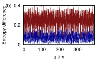
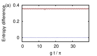
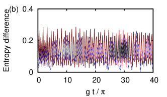
as the system evolves. These differences are plotted against the scaled time $gt/\pi$ in Fig. 1(a) for an initial two-mode squeezed state, and in Fig. 1(b) for a factored product of a CS and atomic ground state $\ket{0}$. From these plots it is evident that $\xi^{\prime}_{\textsc{tei}}$ is in much better agreement with the SLE than with the SVNE over the time interval considered, independent of the parameter values and the nature of the initial state. We therefore choose the SLE as the reference entanglement indicator.

Figure 1: $d_{1}(t)$ (black dashed curve) and $d_{2}(t)$ (pink curve) versus scaled time $gt/\pi$ with $\omega_{F}=1,\omega_{A}=1,\gamma=1$. (a) $g=0.2$, initial squeezed state $\ket{\zeta},\,\zeta=0.1$ (b) $g=100$, initial state $\ket{\alpha}\otimes\ket{0},|\alpha|^{2}=1$.

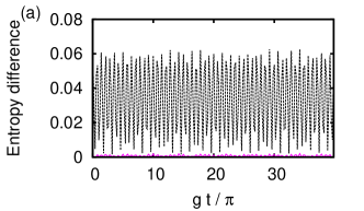
Next, we compare $d_{2}(t)$ with the difference

$$\Delta(t)=|{\text{SVNE}}-{\text{SLE}}|.$$ (22)

We have verified that, In all the cases considered, $\Delta(t)>d_{2}(t)$ (see, for instance, Fig. 2). In what follows, we therefore focus only on $d_{2}(t)$ and the difference

$$d_{3}(t)=|{\text{SLE}}-\xi_{\textsc{ipr}}|.$$ (23)

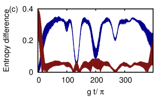
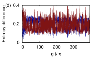
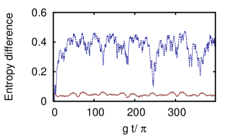
This comparison brings out interesting features of both the indicators. When the strength of the nonlinearity is low relative to that of the coupling (e.g., $\gamma/g=0.01$), it is known sudh_rev_moments that full and fractional revivals occur, and entanglement measures may be expected to display signatures of these revival phenomena. Figure 3 (a) shows that, at the revival time $gT_{\rm rev}/\pi=400$, $\xi^{\prime}_{\textsc{tei}}$ agrees with the SLE much more closely than $\xi_{\textsc{ipr}}$ does. Further, over the entire time interval $(0,T_{\rm rev})$, $d_{2}(t)$ is significantly smaller than $d_{3}(t)$. This feature holds even for larger values of the ratio $\gamma/g$, as may be seen in Fig. 3 (b). $\xi^{\prime}_{\textsc{tei}}$ is therefore to be favored over $\xi_{\textsc{ipr}}$ as an entanglement indicator. The time evolution of the difference $d_{2}(t)$ is drastically different from that of $d_{3}(t)$ for initial field states that depart from ideal coherence. In this case, over the entire time considered, $\xi_{\textsc{ipr}}$ performs significantly better than $\xi^{\prime}_{\textsc{tei}}$ for small values of $\gamma/g$, as in Fig. 3 (c). As the value of $\gamma/g$ is increased, the two indicators have essentially the same behavior, as shown in Fig. 3 (d).

Figure 2: $d_{2}(t)$ (blue dotted curve) and $\Delta(t)$ (pink curve) versus time, with $\omega_{F}=1$, $\omega_{A}=1$, $\gamma=1$, $g=100$, initial state $\ket{\alpha}\otimes\ket{0}$, $|\alpha|^{2}=1$.

Figure 3: $d_{2}(t)$ (blue dotted curve) and $d_{3}(t)$ (brown curve) versus time, with $\omega_{F}=1,\omega_{A}=1,\gamma=1$. (a) $g=100$, initial state $\ket{\alpha}\otimes\ket{0}$ (b) $g=0.2$, initial state $\ket{\alpha}\otimes\ket{0}$ (c) $g=100$, initial state $\ket{\alpha,5}\otimes\ket{0}$ (d) $g=0.2$, initial state $\ket{\alpha,5}\otimes\ket{0}$. $|\alpha|^{2}=1$ in all cases.

We turn now to entangled initial states. In the case of the two-mode squeezed state $\ket{\zeta}$, we see from Figs. 4 (a) and (b) that $\xi^{\prime}_{\textsc{tei}}$ fares much better than $\xi_{\textsc{ipr}}$ over the entire time interval considered, for small values of $\zeta$. With an increase in the value of $\zeta$, both the indicators show comparable departures from SLE.

Figure 4: $d_{2}(t)$ (blue dotted curve) and $d_{3}(t)$ (brown curve) versus time, with $\omega_{F}=1,\omega_{A}=1,\gamma=1,g=0.2$, for the initial two-mode squeezed state $\ket{\zeta}$. (a) $\zeta=0.1$ (b) $\zeta=0.7$.

Figure 5: $d_{2}(t)$ (blue dotted curve) and $d_{3}(t)$ (brown curve) versus time, with $\omega_{F}=1,\omega_{A}=1,\gamma=1,g=0.2$. Initial state $\ket{\psi_{\rm{bin}}}$ with $N=10$.

In the case of an initial binomial state, on the other hand, $\xi_{\textsc{ipr}}$ fares significantly better than $\xi^{\prime}_{\textsc{tei}}$. This can be understood by examining the Hamming distance between the basis states constituting the binomial state. We define this distance in the context of continuous variables by extrapolating the idea of Hamming distance for qudits given below. The Hamming distance between two qubits $\ket{u}$ and $\ket{v}$ ($u,v=0,1$) is $1$ if $u\neq v$, and $0$ if $u=v$. It is evident that this can be extended to qudits in a straightforward fashion. The generalized Hamming distance (see, for instance, ViolaBrown ), i.e., the distance between two bipartite qudit states $\ket{u_{1};u_{2}}$ (where $u_{1},u_{2}=0,1,\dotsc,d-1$) and $\ket{v_{1};v_{2}}$ (where $v_{1},v_{2}=0,1,\dotsc,d-1$), is $0$ if $u_{1}=v_{1}$ and $u_{2}=v_{2}$. The Hamming distance is $1$ if $u_{1}=v_{1}$ and $u_{2}\neq v_{2}$, or vice versa. The distance is $2$ (the maximum possible value in bipartite systems) if $u_{1}\neq v_{1}$ and $u_{2}\neq v_{2}$. Further, the efficacy of $\xi_{\textsc{ipr}}$ as an entanglement indicator increases with an increase in the Hamming distance. This indicator is therefore especially useful for states which are Hamming-uncorrelated (i.e., separated by a Hamming distance equal to 2) ViolaBrown ; HamCorBSSV .

In the case of interest to us, both the subsystems are infinite-dimensional. We would like to examine whether the efficacy of $\xi_{\textsc{ipr}}$ is correlated with the Hamming distance in this case as well. For this purpose, we extend the notion of the Hamming distance between two unentangled basis states in a straightforward manner: The distance between $\ket{m;n}$ and $\ket{p;q}$ (where $m,n,p,q=0,1,2,\dotsc$ ad inf.) is equal to its maximum value of $2$ if $m\neq p$ and $n\neq q$; $1$ if $m=p,n\neq q$ or vice versa; and $0$ if $m=p,n=q$. Note that the binomial state $\ket{\psi_{\rm{bin}}}$ can be expanded as a superposition of states which are Hamming-uncorrelated (Eq. (19)). Figure 5 shows that in this case, too, $\xi_{\textsc{ipr}}$ is a significantly better entanglement indicator than $\xi^{\prime}_{\textsc{tei}}$.

3.2 The double-well BEC model

The effective Hamiltonian for the system (setting $\hbar=1$) is given by sanz

$$H_{\textsc{BEC}}=\omega_{0}N_{\rm{tot}}+\omega_{1}(a^{\dagger}a-b^{\dagger}b)+UN_{\rm{tot}}^{2}-\lambda(a^{\dagger}b+ab^{\dagger}).$$ (24)

$N_{\rm{tot}}=a^{\dagger}a+b^{\dagger}b$ as before, but $(a,a^{\dagger})$ and $(b,b^{\dagger})$ are now the boson annihilation and creation operators of the atoms in wells $A$ and $B$ respectively. $U$ is the strength of the nonlinearity (both in the individual modes as well as in their interaction), $\lambda$ is the linear interaction strength, and $\omega_{0},\omega_{1}$ are constants. As in the previous instance, we select a representative variety of initial states: (i) the unentangled direct product $\ket{\alpha_{a},m_{1}}\otimes\ket{\alpha_{b},m_{2}}$ of boson-added coherent states of atoms in the wells $A$ and $B$ respectively, where $\alpha_{a},\alpha_{b}\in\mathbb{C}$; (ii) the binomial state $\ket{\psi_{\rm{bin}}}$ (Eq. (19)), and (iii) the two-mode squeezed vacuum state $\ket{\zeta}$ (Eq. (20)), with the understanding that the basis states are now product states of the species in the two wells.

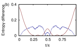
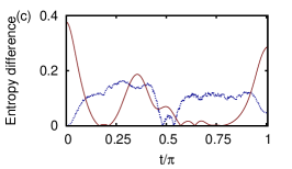
In each of these cases, we must first obtain the state of the system at any time $t\geq 0$ as it evolves under the Hamiltonian $H_{\textsc{BEC}}$. It turns out that, in the case of an initial state of type (i) above, the state of the system can be calculated explicitly as a function of $t$, as outlined in the Appendix. In the cases (ii) and (iii), the state vector at time $t$ is computed numerically. Using the results obtained for the state of the system at time $t$, we have generated, for each of the initial states listed above, tomograms at approximately 1000 instants, separated by a time step 0.001 $\pi/U$. We have verified that, as in the case of the atom-field interaction model, $\xi^{\prime}_{\textsc{tei}}$ agrees better with the SLE than with the SVNE, and that the difference between $\xi^{\prime}_{\textsc{tei}}$ and the SLE is smaller than that between the SVNE and the SLE. In what follows, therefore, we have chosen the SLE as the reference entanglement measure and compared $d_{2}(t)$ with $d_{3}(t)$.

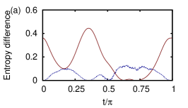
The effective frequency parameter for the linear part of the Hamiltonian $H_{\textsc{BEC}}$ is given (see the Appendix) by $\lambda_{1}=(\omega_{1}^{2}+\lambda^{2})^{1/2}$, while the strength of the nonlinearity is parametrized by $U$. Hence, the relevant ratio for the characterization of the dynamics is $U/\lambda_{1}$. Figure 6 depicts a representative example of the temporal behavior of $d_{2}(t)$ and $d_{3}(t)$. The effect of increasing $U/\lambda_{1}$ can be seen by comparing Figs. 6 (a) and (b), while that of a departure from coherence of the initial state can be seen by comparing (a) and (c).

Figure 6: $d_{2}(t)$ (blue dotted curve) and $d_{3}(t)$ (brown curve) versus time, with $\omega_{0}=1,U=1$. (a) $\omega_{1}=1,\lambda=1$, initial state $\ket{\alpha}\otimes\ket{\alpha}$; (b) $\omega_{1}=0.1,\lambda=0.1$, initial state $\ket{\alpha}\otimes\ket{\alpha}$; (c) $\omega_{1}=1,\lambda=1$, initial state $\ket{\alpha,1}\otimes\ket{\alpha}$. In all cases, $|\alpha|^{2}=1$.

We have also carried out analogous studies in the case of entangled initial states $\ket{\psi_{\rm{bin}}}$ and $\ket{\zeta}$. These results are not presented here owing to limitations of space, but the general trends in the behavior of the entanglement indicators in these cases are consistent with, and corroborate, those found in the atom-field interaction model.

4 Time-series analysis of $d_{1}(t)$

Finally, we turn to an assessment of the long-time behavior of the tomographic entanglement indicator, by means of a detailed time-series analysis.

As we have shown in the foregoing, the deviation of $\xi^{\prime}_{\textsc{tei}}$ from the SVNE is much more pronounced than its deviation from the SLE. It is therefore appropriate to investigate how an initial difference between $\xi^{\prime}_{\textsc{tei}}$ and the SVNE changes with time. With this in mind, a time series of $d_{1}(t)$ has been obtained for each of the models at hand, and used to compute local Lyapunov exponents along the lines customary AbarbanelBook ; NTSA_GP ; abarbanel1992 in the study of dynamical systems. This involves reconstruction of the effective phase space, estimation of the minimum embedding dimension $d_{\rm{emb}}$ of this space, and calculation of the exponents themselves. The procedure used is outlined below.

The time series had 20000 data points. The effective phase space was reconstructed using the TISEAN package tisean . $100$ different initial values $d_{1}(0)$ were randomly chosen in this phase space. The maximum local Lyapunov exponent corresponding to each $d_{1}(0)$ was computed over the same time interval $L$. (The term ‘local’ refers to the fact that $L$ is much smaller than the time interval over which the maximum Lyapunov exponent $\Lambda_{\infty}$ is obtained in the standard method). The average value $\Lambda_{L}$ of these $100$ maximum local Lyapunov exponents was obtained following the prescription in abarbanel1992 . This procedure was repeated for as many as 14 different values of $L$. Further, in each case it was verified that, with an increase in $L$, $\Lambda_{L}$ tends to $\Lambda_{\infty}+(m/L^{q})$, where $m$ and $q$ are constants abarbanel1992 . Note that two neighbouring initial values of the dynamical variable of interest (in our case $d_{1}(t)$) diverges exponentially with the exponent $\Lambda_{L}$ in $L$ steps. We also present the power spectra of the time series for completeness. We would expect a broadband spectra for chaotic data. On the other hand, a spiky power spectra can point to a possible quasi-periodic behaviour. The results are presented below.

4.1 Atom-field interaction model

Figure 7: $\Lambda_{L}$ obtained from the time series of $d_{1}(t)$ (blue crosses) and the fit $\Lambda_{\infty}+(m/L^{q})$ (red curve) versus $L$, with $\omega_{F},\omega_{A}$ and $\gamma$ equal to 1. Initial state $\ket{\alpha}\otimes\ket{0}$: (a) $g=100$, $|\alpha|^{2}=1$ (b) $g=100$, $|\alpha|^{2}=5$ (c) $g=0.2$, $|\alpha|^{2}=1$. (d) Initial state $\ket{\alpha,5}\otimes\ket{0},g=100,|\alpha|^{2}=1$.

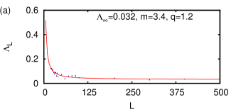
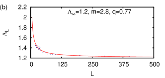
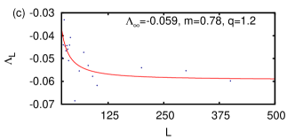
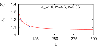
The difference $d_{1}(t)$ has been obtained at each instant with time-step $\delta t=0.1$ for $20000$ time-steps, and the effective phase space has been reconstructed. We see that for both the initial states $\ket{\alpha}\otimes\ket{0}$ and $\ket{\alpha,5}\otimes\ket{0}$ with $|\alpha^{2}|=1$ and weak nonlinearity ($\gamma/g=0.01$), $\Lambda_{L}$ is positive, and both $\Lambda_{L}$ and $\Lambda_{\infty}$ are larger for the second initial state (compare Figs. 7 (a) and (d)). $\Lambda_{\infty}$ increases with an increase in $|\alpha|^{2}$ for the initial state $\ket{\alpha}\otimes\ket{0}$ (compare Figs. 7 (a) and (b)). In contrast, for strong nonlinearity (e.g., as in Fig. 7 (c), $\gamma/g=5$), $\Lambda_{L}$ is negative.

Figure 8: Power spectrum $S(f)$ on a logarithmic scale (red curve) versus $f/g$ for the same respective sets of parameters and initial states as in Figs. 7 (a)–(d).

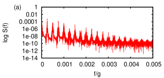
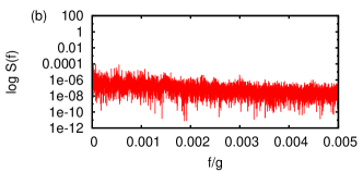
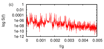
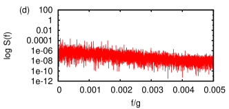
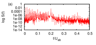
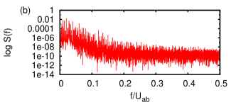
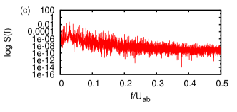
For completeness, we present the power spectrum $S(f)$ of the time series as a function of the frequency $f$ in units of $g$, for each of the cases corresponding to Figs. 7 (a) to (d). The nearly quasi-harmonic power spectrum for weak nonlinearity (Fig. 7 (a)) changes into a broadband spectrum with increasing $|\alpha|^{2}$ (Fig. 7 (b)), while it loses its quasi-harmonicity without becoming a broadband spectrum with increasing nonlinearity (Fig. 7 (c)). The lack of coherence in the initial state makes the power spectrum broadbanded (Fig. 7 (d)).

4.2 The double-well BEC model

Figure 9: $\Lambda_{L}$ obtained from the time series of $d_{1}(t)$ (blue crosses) and the fit $\Lambda_{\infty}+(m/L^{q})$ (red curve) versus $L$, with $\omega_{0}=\omega_{1}=1$. Initial state $\ket{\alpha,1}\otimes\ket{\alpha}$ and (a) hopping frequency $\lambda=5$, $U=0.5$ (b) $\lambda=1$, $U=1$. (c) Initial state $\ket{\alpha,5}\otimes\ket{\alpha,5},\lambda=1,U=1$. $|\alpha|=1$ in all three cases.

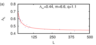
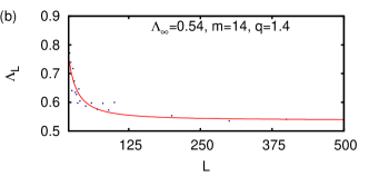
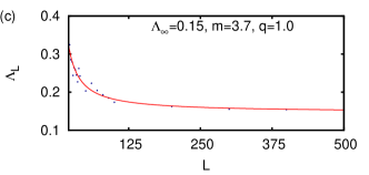
As in the foregoing, we generate the time series of $d_{1}(t)$ by calculating this difference for $20000$ time steps, in this case with $\delta t=0.01$. As seen in Figs. 9 (a)–(c), in this instance $\Lambda_{L}$ is positive regardless of the degree of coherence of the initial states of the subsystems, for a wide range of values of the ratio $U/\lambda_{1}$ (recall that $\lambda_{1}=(\lambda^{2}+\omega_{1}^{2})^{1/2}$). With an increase in $U/\lambda_{1}$, $\Lambda_{\infty}$ increases (Figs. 9 (a), (b)). In contrast to the atom-field interaction model, a departure of the initial state from perfect coherence causes $\Lambda_{\infty}$ to decrease (Figs. 9 (a), (c)).

The power spectra corresponding to the three cases in Fig. 9 are shown in Fig. 10. When the linear part of $H_{\textsc{BEC}}$ is dominant ($\lambda$ dominates over $U$, Fig. 10 (a)), $S(f)$ reflects a degree of quasiperiodicity in the time series. When $U$ becomes comparable to $\lambda$, however, the nonlinearity in the Hamiltonian takes over, and $S(f)$ exhibits a broadband spectrum (Figs. 10 (b), (c)).

Figure 10: Power spectrum $S(f)$ on a logarithmic scale (red curve) versus $f/U$ for the same respective sets of parameters and initial states as in Figs. 9 (a)–(c).

5 Concluding remarks

We have investigated various features of an entanglement indicator for bipartite systems that is obtained solely from tomograms. The performance of this indicator in quantifying the extent of entanglement has been assessed using two model bipartite systems with inherent nonlinearities. It has been shown that the indicator fares significantly better for generic initial states of the system even during temporal evolution, compared to better-known entanglement indicators such as one based on inverse participation ratios. In order to quantify the reliability of the indicator over long intervals of time, the difference between the SVNE and our tomographic indicator has been examined using a time-series analysis. The manner in which this difference is sensitive to the nonlinearity of the system, the nature of the interaction, and the precise initial state is revealed by the time-series analysis. The importance and relevance of this investigation lies in the fact that detailed state reconstruction from the tomogram is completely avoided in identifying an efficient entanglement indicator for generic bipartite systems involving continuous variables.

Appendix: Time evolution in the double-well BEC model

The double-well BEC effective Hamiltonian is given by Eq. (24). We require the state $\ket{\psi(t)}$ corresponding to an initial state that is a direct product of normalized boson-added coherent states of the atoms in the wells $A$ and $B$, namely,

$$\ket{\psi_{m_{1},m_{2}}(0)}=\ket{\alpha_{a},m_{1}}\otimes\ket{\alpha_{b},m_{2}},$$ (25)

where $\alpha_{a},\alpha_{b}\in\mathbb{C}$ and $m_{1},m_{2}$ are non-negative integers. The dependence of the state on $\alpha_{a}$ and $\alpha_{b}$ has been suppressed on the left-hand side for notational simplicity. The $m$-PACS $\ket{\alpha,m}$ (defined in Eq. (17)) reduces to the standard oscillator coherent state $\ket{\alpha}$ for $m=0$.

In the special case $m_{1}=0,m_{2}=0$, the state at any time $t$ corresponding to the initial state $\psi_{0,0}(0)$ has been shown in Ref. sanz to be given by

$$\ket{\psi_{00}(t)}= e^{-\tfrac{1}{2}(|\alpha_{a}|^{2}+|\alpha_{b}|^{2})}\sum_{p,q=0}^{\infty}\frac{\beta_{1}^{p}(t)\,\beta_{2}^{q}(t)}{\sqrt{p!q!}}$$

$$e^{-it(p+q)[\omega_{0}+U(p+q)]}\ket{p}\otimes\ket{q},$$ (26)

where

$$\left.\begin{array}[]{lll}\beta_{1}(t)&=&\alpha_{a}\cos\,(\lambda_{1}t)+(i/\lambda_{1})(\lambda\alpha_{b}-\omega_{1}\alpha_{a})\sin\,(\lambda_{1}t),\\[4.0pt] \beta_{2}(t)&=&\alpha_{b}\cos\,(\lambda_{1}t)+(i/\lambda_{1})(\lambda\alpha_{a}+\omega_{1}\alpha_{b})\sin\,(\lambda_{1}t),\end{array}\right\}$$ (27)

and $\lambda_{1}=(\lambda^{2}+\omega_{1}^{2})^{1/2}$. It can then be shown sharmila that the state vector at time $t$ is given by

$$\ket{\psi_{m_{1},m_{2}}(t)}=M_{m_{1},m_{2}}(t)\ket{\psi_{00}(t)},$$ (28)

where the operator $M_{m_{1},m_{2}}(t)$ is as follows. Let $k,l,p,q$ denote non-negative integers, and let

$$s=k+l+p+q,\,\overline{p}=(k+m_{2}-l),\,\overline{q}=(l+m_{1}-k).$$ (29)

Further, let

$$\kappa=\big{[}m_{1}!m_{2}!L_{m_{1}}(-|\alpha_{a}|^{2})L_{m_{2}}(-|\alpha_{b}|^{2})\big{]}^{-1/2}$$ (30)

and $\Gamma=\cos^{-1}(\omega_{1}/\lambda_{1})$. Then

$$M_{m_{1},m_{2}}(t) = \kappa\Big{\{}\sum_{k=0}^{m_{1}}\sum_{l=0}^{m_{2}}\sum_{p=0}^{\overline{p}}\sum_{q=0}^{\overline{q}}(-1)^{k-p}{\tbinom{m_{1}}{k}}{\tbinom{m_{2}}{l}}\,{\tbinom{\overline{p}}{p}}\,{\tbinom{\overline{q}}{q}}\,e^{2i(l-k)\lambda_{1}t}\times$$ (31)

$$(\cos\,\tfrac{1}{2}\Gamma)^{s}(\sin\,\tfrac{1}{2}\Gamma)^{2(m_{1}+m_{2})-s}(a^{\dagger})^{p+\overline{q}-q}\,(b^{\dagger})^{q+\overline{p}-p}\Big{\}}\times$$

$$e^{-i\omega_{0}t(m_{1}+m_{2})+i\lambda_{1}t(m_{1}-m_{2})}e^{-iUt(m_{1}+m_{2})(2N_{\rm{tot}}+m_{1}+m_{2})}.$$