APXReferences \TheoremsNumberedThrough\ECRepeatTheorems\EquationsNumberedThrough
Lam and Qian
Bounding Optimality Gap via Bagging
Bounding Optimality Gap in Stochastic Optimization via Bagging: Statistical Efficiency and Stability
Henry Lam \AFFDepartment of Industrial Engineering and Operations Research, Columbia University, New York, NY 10027, \EMAILkhl2114@columbia.edu \AUTHORHuajie Qian \AFFDepartment of Industrial Engineering and Operations Research, Columbia University, New York, NY 10027, \EMAILh.qian@columbia.edu
We study a statistical method to estimate the optimal value, and the optimality gap of a given solution for stochastic optimization as an assessment of the solution quality. Our approach is based on bootstrap aggregating, or bagging, resampled sample average approximation (SAA). We show how this approach leads to valid statistical confidence bounds for non-smooth optimization. We also demonstrate its statistical efficiency and stability that are especially desirable in limited-data situations, and compare these properties with some existing methods. We present our theory that views SAA as a kernel in an infinite-order symmetric statistic, which can be approximated via bagging. We substantiate our theoretical findings with numerical results.
stochastic optimization, optimality gap, bagging, symmetric statistics, solution validation
1 Introduction
Consider a stochastic optimization problem
| (1) |
where is the decision space, is generated under some distribution , and denotes its expectation. We focus on the situations where is not known, but instead a collection of i.i.d. data for , say , are available. Obtaining a good solution for (1) under this setting has been under active investigation both from the stochastic and the optimization communities. Common methods include the sample average approximation (SAA) (Shapiro et al. (2009), Kleywegt et al. (2002), Higle et al. (1996)), stochastic approximation (SA) or gradient descent (Kushner and Yin (2003), Borkar (2009), Nemirovski et al. (2009)), and (distributionally) robust optimization (Delage and Ye (2010), Bertsimas et al. (2018), Wiesemann et al. (2014), Ben-Tal et al. (2013)). These methods aim to find a solution that is nearly optimal, or in some way provide a safe approximation. Applications of the generic problem (1) and its data-driven solution techniques span from operations research, such as inventory control, revenue management, portfolio selection (see, e.g., Shapiro et al. (2009), Birge and Louveaux (2011)) to risk minimization in machine learning (e.g., Friedman et al. (2001)).
This paper concerns the estimation of using limited data. Moreover, given a solution, say , a closely related problem is to estimate the optimality gap
| (2) |
This allows us to assess the quality of , in the sense that the smaller is, the closer is the solution to the true optimum in terms of achieved objective value. More precisely, we will focus on inferring a lower confidence bound for , and, correspondingly, an upper bound for - noting that its first term can be treated as a standard population mean of that is estimable using a sample independent of the given , or that can be represented as the max of the expectation of whose estimation is structurally the same as .
This problem is motivated by the fact that many state-of-the-art solution methods mentioned before are only amenable to crude, worst-case performance bounds. For instance, Shapiro and Nemirovski (2005) and Kleywegt et al. (2002) provide large deviations bounds on the optimality gap of SAA in terms of the diameter or cardinality of the decision space and the maximal variance of the function . Nemirovski et al. (2009) and Ghadimi and Lan (2013) provide bounds on the expected value and deviation probabilities of the SA iterates in terms of the strong convexity parameters, space diameter and maximal variance. These bounds can be refined under additional structural information (e.g., Shapiro and Homem-de-Mello (2000)). While they are very useful in understanding the behaviors of the optimization procedures, using them as a precise assessment on the quality of an obtained solution may be conservative. Because of this, a stream of work studies approaches to validate solution performances by statistically bounding optimality gaps. Mak et al. (1999), Bayraksan and Morton (2006), Love and Bayraksan (2015) and Shapiro (2003) investigate the use of SAA to estimate these bounds. Lan et al. (2012) validate the performances of SA iterates by using convexity conditions. Stockbridge and Bayraksan (2013) and Partani et al. (2006) study approaches like the jackknife and probability metric minimization to reduce the bias in the resulting gap estimates. Bayraksan and Morton (2011) utilize gap estimates to guide sequential sampling. Duchi et al. (2021), Blanchet et al. (2019) and Lam and Zhou (2017) investigate the use of empirical and profile likelihoods to estimate optimal values. Our investigation in this paper follows the above line of work on solution validation, focusing on the situation when data are limited and hence the statistical efficiency becomes utmost important. We also point out a related series of work that validate feasibility under uncertain constraints (e.g., Luedtke and Ahmed (2008), Pagnoncelli et al. (2009), Wang and Ahmed (2008), Carè et al. (2014), Calafiore (2017), Lam and Qian (2019), Hong et al. (2021)), though their problem of interest is beyond the scope of this paper as we focus on deterministically constrained problems and objective value performances.
More precisely, we introduce a bootstrap aggregating, or commonly known as bagging (Breiman (1996)), approach to estimate a lower confidence bound for . This comprises repeated resampling of data to construct SAAs, and ultimately averaging the resampled optimal SAA values. We demonstrate how this approach applies under very general conditions on the cost function and decision space , while enjoys high statistical efficiency and stability. Compared to procedures based on batching (e.g., Mak et al. (1999)), which also have documented benefits in wide applicability and stability, the data recycling in our approach provably improves a tradeoff between the tightness of the resulting bound and the statistical accuracy encountered in batching. In cases where sufficient smoothness is present and central limit theorem (CLT) for SAA (e.g., Shapiro et al. (2009), Bayraksan and Morton (2006)) can be directly applied, we also see that our approach gains stability regarding standard error estimation, thanks to the smoothing effect brought by bagging. Nonetheless, our approach generally requires higher computational load than these previous methods due to the need to solve many resampled programs, which can be viewed as the price to pay for all these statistical gains.
The theoretical justification of our bagging scheme comes from viewing SAA as a kernel in an infinite-order symmetric statistic (Frees (1989)), and an established optimistic bound for SAA as its asymptotic limit. A symmetric statistic is a generalization of sample mean in which each summand consists of a function (i.e., kernel) acting on more than one observation (Serfling (2009), Lee (1990)). In particular, the size of the SAA program can be seen as precisely the kernel “order” (or “degree”), which depends on the data size and is consequently of an infinite-order nature. Our bagging scheme serves as a Monte Carlo approximation for this symmetric statistic. As a main methodological contribution, we analyze the asymptotic behaviors of the statistic and the resulting bounds as the SAA size grows, and translate them into efficient performances of our bagging scheme. Finally, we note that the notion of infinite-order symmetric statistics has been used in analyzing ensemble machine learning predictors like random forests (Wager and Athey (2018)); our SAA kernels are, from this view, in parallel to the base learners in the latter context.
Finally, we mention that Eichhorn and Römisch (2007) has also studied the resampling of SAA programs to construct confidence intervals for the optimal values of stochastic programs. Our approach connects with, but also differs substantially from Eichhorn and Römisch (2007) in several regards. In terms of scope of applicability, Eichhorn and Römisch (2007) focuses on mixed-integer linear programs, while we consider cost functions that can be generally non-Donsker. In terms of methodology, Eichhorn and Römisch (2007) utilizes the quantiles of the resampled distribution to generate confidence intervals, by observing the same limiting distribution between an original CLT and the bootstrap CLT. The resampling in Eichhorn and Römisch (2007) applies when the optimal solution is unique, or otherwise requires a “two-layer” extended bootstrap where each resample is drawn from a new sample of the true distribution (as opposed to most bootstrap methods that allow repeated resample from the same original sample, with the availability of a conditional bootstrap CLT). The latter requires substantial data size or resorting to subsampling. Our bagging approach, in contrast, is based on a direct use of Gaussian limit and standard error estimation in the CLT for the optimistic bound. Our burden lies on the bootstrap Monte Carlo size requirement to obtain consistent standard error estimate, and less on the data size requirement. Relatedly, there is an orthogonal line of works on resampling approaches to estimate solution errors for randomized algorithms such as stochastic gradient descent (Fang (2019), Fang et al. (2018)) and Newton’s methods (Chen and Lopes (2020), Lopes et al. (2018)). These works however treat the data as deterministic and focus on the quantification of algorithmic uncertainties. Last but not least, during the review process of this paper, Chen and Woodruff (2022) implemented an open-source software for bootstrap estimation in stochastic programs, based on our proposed scheme as well as Eichhorn and Römisch (2007), and demonstrated numerical performances in extensive experiments.
We summarize our contributions of this paper as follows:
-
1.
Motivated from the challenges of existing techniques (Section 2), we introduce a bagging procedure to estimate a lower confidence bound for , correspondingly an upper confidence bound for (Section 3). We present the idea of our procedure that views SAA as a kernel in a symmetric statistic, and an optimistic bound for SAA as its associated limiting quantity (Section 4).
-
2.
We analyze the asymptotic behaviors of our bagging estimator, which can be viewed as an infinite-order symmetric statistic, under three increasingly stringent sets of regularity conditions on the optimization problem: minimal smoothness requirements, Lipschitzness and additionally solution uniqueness. In the last case, we also demonstrate how our asymptotic is on par with the classical CLT on SAA. These results are presented in Section 5. The mathematical developments without smoothness conditions utilize a combination of an analysis-of-variance (ANOVA) decomposition of the symmetric statistic and an analysis of the high-order error of the Hajek projection (Van der Vaart (2000)), using a probabilistic coupling argument and the Efron-Stein inequality (Appendix 11). The developments with smoothness conditions and the reconciliation of the classical CLT on SAA use the argmax theorem and a maximal deviation bound for empirical processes (Appendix 12).
-
3.
Building on the above results, we demonstrate that the bounds generated from our bagging procedure exhibit asymptotically correct coverages. In deriving these guarantees, we also analyze and formulate sufficient conditions on the bootstrap Monte Carlo sizes. These developments are in Section 6, with additional technical details in Appendices 9, 13 and 14.
-
4.
We compare our approach with both batching and the direct use of CLT. In particular, we show that our bagging estimator possesses a standard error no larger than both of these competing methods whenever applicable (i.e., bagging offers variance reduction). These developments are in Sections 7, with mathematical details in Appendix 15. Tying to our beginning motivation, we then argue how bagging improves a tradeoff between the bound tightness and the statistical accuracy faced by batching, and elicits more stable standard error estimates than the direct use of CLT. We support these comparisons by our numerical experiments (Section 8).
2 Existing Challenges and Motivation
We discuss some existing methods and their challenges, to motivate our investigation. We start the discussion with the direct use of asymptotics from sample average approximation (SAA).
2.1 Using Asymptotics of Sample Average Approximation
When the cost function in (1) is smooth enough, it is known classically that a central limit theorem (CLT) governs the behavior of the estimated optimal value in SAA, namely
| (3) |
We first introduce the following Lipschitz condition:
[Lipschitz continuity in the decision] The cost function is Lipschitz continuous with respect to , in the sense that
for any , where denotes the norm and satisfies .
Denote “” as convergence in distribution. The following result is taken from Shapiro et al. (2009):
Theorem 2.1 (Extracted from Theorem 5.7 in Shapiro et al. (2009))
Roughly speaking, Theorem 2.1 stipulates that, under the depicted conditions, one can use (4) to obtain
| (5) |
as a valid lower confidence bound for (and analogously for given ), where is some suitable error term that captures the quantile of the limiting distribution in (4). Indeed, in the case of estimating , Bayraksan and Morton (2006) provides an elegant argument that shows that, to achieve confidence, one can take where is the standard normal critical value and is a standard deviation estimate, regardless of whether the limit in (4) is a Gaussian distribution. Bayraksan and Morton (2006) calls this the single-replication procedure. More precisely, a straightforward modification of their procedure (which focuses on bounding ) to bounding the optimal value computes the by , where is the solution from (3) and .
Though Theorem 2.1 (and other related work, e.g., Dentcheva et al. (2017), Kleywegt et al. (2002)) is very useful, if the SAA solutions have a “jumping” behavior, namely that program (1) has several near-optimal solutions with hugely differing objective variances, then the standard deviation estimate needed in the bound (5) can be unreliable. This is because depends heavily on , which can fall close to any of the possible near-optimal solutions with substantial chance and make the resulting estimation noisy. This issue is illustrated in, e.g., Examples 1 and 2 in Bayraksan and Morton (2006).
We should also mention that, as an additional issue, the bias in relative to can be quite large in any given problem, i.e., arbitrarily close to order described in the CLT, even if all the conditions in Theorem 2.1 hold (Partani (2007)). Note that this bias is in the optimistic direction (i.e., the resulting bound is still correct, but conservative), and it also appears in the “optimistic bound” approach that we discuss next. There have been techniques such as the jackknife (Partani (2007), Partani et al. (2006)) and probability metric minimization (Stockbridge and Bayraksan (2013)) in reducing this bias effect.
2.2 Batching Procedures
An alternative approach is to use the optimistic bound (Mak et al. (1999), Shapiro (2003), Glasserman (2013))
| (6) |
where in (6) is taken with respect to the data in constructing the SAA value . The bound (6) holds for any , as a direct consequence from Jensen’s inequality in exchanging the expectation and the minimization operator in the SAA.
The bound (6) offers a simple way to construct a lower bound for under great generality. Note that the left hand side of (6) is a mean of SAA. Thus, if one can “sample” a collection of SAA values, then a lower confidence bound for can be constructed readily by using a standard estimate of population mean. To “sample” SAA values, an approach suggested by Mak et al. (1999) is to batch i.i.d. data set into say batches, each batch consisting of observations, so that (we ignore rounding issues). For each , solve an SAA using the observations in the -th batch; call this value . Then use
| (7) |
where and are the sample mean and variance from , and is the -level standard normal quantile.
The bound (7) does not rely on any continuity of , and is simply the sample standard error for a sample mean. This bound largely mitigates the aforementioned unstable estimation encountered in bounds that directly use the SAA asymptotic (4). Nonetheless, there is an intrinsic tradeoff between the bound tightness and statistical accuracy. On one hand, must be chosen big enough (e.g., roughly ) so that one can use the CLT to justify the approximation (7). On the other hand, the larger is , the closer is to in (6), leading to a tighter lower bound for . This is thanks to a monotonicity property in that is non-decreasing in (Mak et al. (1999), Norkin et al. (1998)). Therefore, there is a tradeoff between the statistical accuracy controlled by (in terms of the validity of the CLT) and the tightness controlled by (in terms of the position of in (6)). In the batching or the so-called multiple-replication approach of Mak et al. (1999), this tradeoff is confined to the relation . There have been suggestions to improve this tradeoff, e.g., by using overlapping batches (Love and Bayraksan (2015, 2011)), but their validity requires uniqueness or exponential convergence of the solution (e.g., in discrete decision space).
2.3 Motivation and Overview of Our Approach
Thus, in general, when the sample size is small, the batching approach appears to necessarily settle for a conservative bound in order to retain statistical accuracy. The starting motivation for the bagging procedure that we propose next is to break free this tightness-accuracy tradeoff. In particular, we offer a bound roughly in the form
| (8) |
where is a point estimate obtained from bagging many resampled SAA values, and signifies the size of the resampled SAA (i.e., the “bags”). The quantity relies on a standard error estimate of . Table 1 highlights the differences between our bagging bound and direct-CLT and batching bounds, which we explain further below.
| Direct-CLT bound | Batching bound | Bagging bound | ||||||||
|
|
|
||||||||
|
No | No | Yes | |||||||
|
No | Yes | Yes | |||||||
|
|
None | None | |||||||
| #SAAs to solve |
|
Compared to batching, our method shares the same advantages that the standard error term does not succumb to the “jumping” solution behavior, and our bound holds regardless of the continuity to the decision. Moreover, our bagging point estimate has provably no larger variance than the batching point estimate and, as described above, it allows using a resampled SAA size that is larger than the batched SAA size.
Compared to direct-CLT, our bound would be almost as tight by choosing the resample size in (8) to be arbitrarily close to the order of . Moreover, our standard error term is more stable than the counterpart in (5) thanks to the use of many resampled SAAs rather than a single SAA. Furthermore, our approach works under conditions more general than when (5) is applicable, and if we re-impose Lipschitz continuity on the decision required for (5), then our bagging point estimator has no larger asymptotic variance than in (5), with strictly smaller asymptotic variance in the case of multiple optima. In the case of unique optimum, the resample size is allowed to be the same order as in which case our bagging bound achieves the same level of tightness as direct-CLT.
Despite the above advantages, our approach requires solving a number of resampled SAA programs that is of larger order than the data size (reduced to larger order than if a bias correction is applied to the variance estimator), and is thus computationally more costly than batching and direct-CLT methods. The higher computation cost is the price to pay to elicit our benefits depicted above. Our approach is thus most recommended when statistical performance is of higher concern than computation efficiency, prominently in small-sample situations.
The next section will explain our procedure in more detail. A key insight is to view SAA as a symmetric kernel and the optimistic bound (6) as a limiting quantity of an associated symmetric statistic, which can be estimated by bagging.
3 Bagging Procedure to Estimate Optimal Values
This section presents our approach. Instead of batching the data, we uniformly resample observations from for many, say , times. We use each resample to form an SAA problem and solve it. We then average all these resampled SAA optimal values. The resampling can be done with or without replacement (we will discuss some differences between the two). We summarize our procedure in Algorithm 1.
| (9) |
| (10) |
In the output of Algorithm 1, the first term is the average of many bootstrap resampled SAA values, which resembles a bagging predictor by viewing each SAA as a “base learner” (Breiman (1996)). The quantity in (10) is the covariance between the count of a specific observation in a bootstrap resample, denoted , and the resulting resampled SAA value . The quantity is an empirical version of the so-called infinitesimal jackknife (IJ) estimator (Efron (2014)), which has been used to estimate the standard error of bagging schemes, including in random forests or tree ensembles (Wager et al. (2014)). The additional constant factor in the second line of (9) is a correction specific to resampling without replacement that is required for consistency in the asymptotic regime where is of the same order as .
4 SAA as Symmetric Kernel
We explain how Algorithm 1 arises. In short, the in Algorithm 1 acts as a point estimator for in the optimistic bound (6), whereas captures the standard error in using this point estimator.
To be more precise, let us introduce a functional viewpoint and write
| (11) |
where
is the SAA value, expressed more explicitly in terms of the underlying data used. Here, the expectation is generated with respect to i.i.d. variables , i.e., denotes the product measure of ’s. For convenience, we denote as the expectation either with respect to or the product measure of ’s when no confusion arises. Also, we denote .
With these notations, the optimistic bound (6) can be expressed as
with the best bound being thanks to the monotonicity property of the expected SAA value mentioned before.
Suppose that we have used sampling with replacement in Algorithm 1. Also say we use infinitely many bootstrap replications, i.e., . Then, the estimator in Algorithm 1 becomes precisely
where is the empirical distribution formed by , i.e., where is the delta measure at . If is “smooth” in some sense, then one would expect to be close to . Indeed, when is fixed, , which is expressible as the -fold expectation under in (11), is multi-linear, i.e.,
and is always differentiable with respect to (in the Gateaux sense) from the theory of von Mises statistical functionals (Serfling (2009)). This ensures that is close to probabilistically, as elicited by a CLT (Theorem 4.1 below).
Note that is exactly the average of over all possible combinations of drawn with replacement from . This is equivalent to
| (12) |
which is the so-called -statistic. If we have used sampling without replacement in Algorithm 1, we arrive at the estimator (assuming again )
| (13) |
where denotes the collection of all subsets of size in . The quantity (13) is known as the -statistic. The and estimators in (12) and (13) both belong to the class of symmetric statistics (Serfling (2009), Van der Vaart (2000), De la Pena and Giné (2012)), since the estimator is unchanged against a shuffling of the ordering of the data . Correspondingly, the function is known as the symmetric kernel. Symmetric statistics generalize the sample mean, the latter corresponding to the case when .
When , then and above are approximated by a random sampling of the summands on the right hand side of (12) and (13). These are known as incomplete - and -statistics (Lee (1990), Blom (1976), Janson (1984)), and are precisely our . As is chosen large enough, will well approximate and .
To discuss further, we make the following assumptions: {assumption}[-boundedness] We have
Denote . Also denote as the variance under . {assumption}[Finite non-zero variance] We have .
We have the following asymptotics of and :
Theorem 4.1
Proof 4.2
Theorem 4.1 is a consequence of the classical CLT for symmetric statistics. The expression , as a function defined on the space , is the so-called influence function of , which can be viewed as its functional derivative with respect to (Hampel (1974)). Alternately, for a -statistic , the expression is the so-called Hajek projection (Van der Vaart (2000)), which is the projection of the statistic onto the subspace generated by the linear combinations of for any measurable function . It turns out that these two views coincide, and the - and -statistics (whose approximation uses the projection viewpoint and the functional derivative viewpoint respectively) obey the same CLT as depicted in Theorem 4.1.
The output of Algorithm 1 is now evident given Theorem 4.1. When , is precisely under sampling without replacement or under sampling with replacement. The quantity in Algorithm 1, an empirical IJ estimator, can be shown to approximate the asymptotic variance as , by borrowing recent results in bagging (Efron (2014), Wager and Athey (2018)) (Theorems 6.1 and 6.2 below show stronger results). Then the procedural output is the standard CLT-based lower confidence bound for .
The discussion above holds for a fixed , the sample size used in the resampled SAA. It also shows that, at least asymptotically, using with or without replacement does not matter. However, using a fixed regardless of the size of is restrictive and leads to conservative bounds. The next subsection will relax this requirement and present results on a growing against , which in turn allows us to get a tighter in the optimistic bound (6).
5 Asymptotic Behaviors with Growing Resample Size
We first make the following strengthened version of Assumption 4: {assumption}[-bounded modulus of continuity] We have
where are i.i.d. generated from .
Assumption 5 holds quite generally, for instance under any of the following sufficient conditions: {assumption}[Uniform boundedness] is uniformly bounded over .
[Uniform Lipschitz condition] is Lipschitz continuous with respect to , where the Lipschitz constant is uniformly bounded in , i.e.,
where is some norm in . Moreover, .
[Majorization]
where . That Assumption 5 implies Assumption 5 is straightforward. To see how Assumption 5 implies Assumption 5, note that, if the former is satisfied, we have
Similarly, Assumption 5 implies Assumption 5 because the former leads to
We have the following asymptotics:
Theorem 5.1 (CLT for growing resample size under sampling without replacement)
Theorem 5.2 (CLT for growing resample size under sampling with replacement)
Theorems 5.1 and 5.2 are analogs of Theorem 4.1 when grows with . In both theorems, we see that there is a limit in how large we can take relative to , which is thresholded at roughly order and for and respectively. A symmetric statistic with a growing is known as an infinite-order symmetric statistic (Frees (1989)), and has been harnessed in analyzing random forests (Mentch and Hooker (2016), Wager et al. (2014), Wager and Athey (2018)). Theorems 5.1 and 5.2 give the precise conditions under which the SAA kernel results in an asymptotically converging infinite-order symmetric statistic. In particular, the requirement in Theorem 5.1 implies that, asymptotically, we can use almost the full data set to construct the resampled SAA in .
We obtain Theorem 5.1 by looking at the variance of via an analysis-of-variance (ANOVA) decomposition (Efron and Stein (1981)) of the symmetric kernel . Thanks to the uncorrelatedness among the ANOVA terms, we can control the higher-order variance of at by using a bound from Wager and Athey (2018). However, unlike in Theorem 4.1 where a clean CLT is available as the first-order effect dominates the higher-order ones, the first-order effect may become degenerate (i.e., tend to 0) as grows, and the growth conditions in Theorem 5.1 allows obtaining a normality asymptotic with the term. From Theorem 5.1, the conclusion of Theorem 5.2 follows by using a relation between - and -statistics in the form
| (17) |
where and is the average of all with at least two of being the same (see, e.g., Section 5.7.3 in Serfling (2009)). By carefully controlling the difference between and , one can show an asymptotic for under a slower growth rate of . This leads to a slightly less general result for in Theorem 5.2. The proofs of Theorems 5.1 and 5.2 are both in Appendix 11.
Corollary 5.3 (Exact CLT for growing resample size under non-degeneracy)
Non-degeneracy of the limit variance depends on the intricate interplay between the SAA optimal solution and the cost function, and thus may not be easily verified in general. For Lipschitz problems, however, the limit variance can be compactly characterized in terms of the cost function and minimizers of an associated Gaussian process.
Theorem 5.4 (Characterization of limit variance under Lipschitzness)
Suppose Assumptions 2.1, 4 and 5 hold, and that the decision space is compact. Let be a centered Gaussian process on , the set of optimal solutions for (1), with covariance defined by for any . Then there exists a random variable on the same probability space as the Gaussian process such that almost surely and that
| (18) |
where and are independent. Therefore, the non-degeneracy condition holds if and only if . Alternatively, the limit variance can also be represented in terms of the covariance kernel, , where is an independent copy of .
Theorem 5.4 shows that the limit variance is exactly the variance of the cost after being averaged over random minimizers of the limit Gaussian process on , or equivalently, the expected covariance kernel over a pair of independent minimizers. Theorem 5.4 is proved by first utilizing SAA asymptotic theories and uniform integrability of the SAA kernel to shrink the decision space from to the set of optima , and then relating the limit variance to the cost function and minimizers of the limit Gaussian process through a coupling argument and an application of the argmax theorem from empirical process theory.
In order to demonstrate the generality of the non-degeneracy condition as implied by Theorem 5.4, we consider general convex problems on and apply Theorem 5.4 to derive more transparent conditions for non-degeneracy.
Theorem 5.5 (Non-degeneracy for convex problems)
Assume the conditions of Theorem 5.4. Let the decision space be a compact convex set, be convex in for each , and be the minimizer of the limit Gaussian process from Theorem 5.4. Then is an optimal solution by convexity, and . Therefore non-degeneracy holds if and only if . In particular, a sufficient condition for non-degeneracy is that for every optimal solution, or even more stringently, for every feasible solution .
The last conclusion of Theorem 5.5 stipulates that for convex problems, non-degeneracy of our bagging estimator can be guaranteed simply by having a noisy objective at every feasible solution. More generally, Theorem 5.5 concludes that non-degeneracy is guaranteed by having a noisy objective at every optimal solution, and even more generally boils down to a noisy objective at , which can be viewed as a “bagged optimal solution”. This link between the non-degeneracy of a bagged optimal value and the non-zero objective variance at a bagged optimal solution arises from the fact that a convex objective must be linear in when restricted to the (convex) set of optima , and therefore the expectation operation and the application of the cost function are exchangeable, i.e., . We illustrate the application of Theorem 5.5 to two convex programs below. For both examples, we assume the basic required conditions (i.e., Assumptions 2.1, 4 and 5) hold.
Example 5.6
Consider , and a linear cost , where has mean zero and covariance matrix . Then , and a sufficient condition for non-degeneracy is that for every optimal solution . For example, that is non-singular and is sufficient because every optimal solution must then be on the boundary (hence nonzero) and thus have a strictly positive objective variance. If , however, the problem becomes degenerate as .
Example 5.7
Let be an arbitrary compact convex set, and where is a convex and strictly increasing function. Note that is convex in because it is the composition of a convex and increasing function and a convex function. Theorem 5.5 then entails that a sufficient condition for non-degeneracy is that is not supported on any -sphere, i.e., set in the form of for and , since it implies for each that and hence by the strict monotonicity of .
We also point out that, since the limit variance is the same as the objective variance at the bagged optimal solution as stated in Theorem 5.5, it follows that the bound , where the point estimate is the full SAA optimal value from (5) and the standard error term is from our bagging bound in Algorithm 1, is a valid confidence bound by a similar argument from Bayraksan and Morton (2006) for justifying the single-replication procedure. To briefly explain, we have by optimality, where , and hence . This bound combines the advantages of both bagging and direct-CLT bounds: Compared to (5), it is conjectured to have a stabler and smaller standard error term (thanks to the discussion in the next section) and compared to our bagging bound it has a tighter point estimate. However, this bound is guaranteed to be valid only for convex problems.
Next we show yet another refinement when, in addition to Lipschitzness, the optimal solution is also unique. Under this additional assumption, Theorem 5.4 immediately forces the limit variance to be , where is the unique optimum. Our bagging estimator thus elicits the same CLT as Theorem 2.1. To state the next result, we define:
Definition 5.8 (Essential uniqueness)
We say (1) has essentially unique optimal solution if almost surely for any two optimal solutions .
Essential uniqueness is more general than the usual uniqueness in that it allows multiple optimal solutions as long as they perform exactly the same under any possible scenario of the uncertain quantity, and hence enhances the applicability of our next result. More importantly, it is both a sufficient and necessary condition to ensure the SAA weak limit in (4) is Gaussian; otherwise, the limit is the minimum of a Gaussian process that triggers a strict variance reduction property of our approach (see Theorem 7.2 in the sequel). The next result is as follows:
Theorem 5.9 (Recovery of the classical CLT for SAA under solution uniqueness)
Suppose Assumptions 2.1, 4 and 5 hold, that the decision space is compact, and that (1) has essentially unique optimal solution. Let be an optimal solution and assume . We have for arbitrary choices of . Moreover, as , and if for some constant we have
| (19) |
where is normal with mean zero and variance .
Note that, compared with Theorems 5.1 and 5.2, the centering quantity in (19) is changed from to . The asymptotic distribution is Gaussian with variance precisely the objective variance at . This gives rise to the same CLT as Theorem 2.1 in the special case where (1) has essentially unique optimal solution, and in particular when the set of optima is a singleton . If the essential uniqueness condition does not hold, there could be a discrepancy between the optimistic bound and (This can be hinted by observing the different types of limits between Theorems 5.1, 5.2 and Theorem 2.1, namely Gaussian versus the minimum of a Gaussian process).
We obtain Theorem 5.9 from a more delicate control of the high-order variance components in the ANOVA decomposition and an analysis on the negligible bias of with respect to the true optimal value , both of which are related to the maximal deviation of an empirical process generated by the centered cost function indexed by the decision, i.e., . The Lipschitz assumption allows us to estimate this maximal deviation using empirical process theory. Appendix 12 shows the proof details for Theorems 5.4, 5.5 and 5.9.
6 Error Estimates and Coverages
With the limit theorems in Sections 4 and 5, we now derive the coverage guarantees for the output from Algorithm 1. In doing so, we incorporate two additional developments. One is the analysis of the IJ estimator in approximating the standard error. Second is the analysis of the Monte Carlo error in running the bootstrap with a finite number of replications. First, we have the following consistency of the IJ variance estimator, relative to the magnitude of the target standard error:
Theorem 6.1 (Consistency of IJ estimator under resampling without replacement)
Consider resampling without replacement. In either of the following cases:
- •
- •
the IJ variance estimator is consistent up to a negligible error, i.e.
Theorem 6.2 (Consistency of IJ estimator under resampling with replacement)
Theorem 6.1 is justified by adopting the arguments for random forests in Wager and Athey (2018) and a weak law of large numbers, and Theorem 6.2 follows from analyzing the difference between - and -statistics as in the proof of Theorem 5.2. Appendix 13 shows the details.
When a large enough bootstrap size is used in Algorithm 1, the Monte Carlo errors in estimating the point estimator and its variance both vanish. This gives an overall coverage guarantee for the output of our bagging procedure, as in the next theorem:
Theorem 6.3 (CLT for Algorithm 1)
In the case of resampling without replacement, assume either 1) Assumptions 4 and 5 hold and , or 2) Assumptions 2.1, 4 and 5 hold, the decision space is compact, (1) has essentially unique optimal solution and for some constant . In the case of resampling with replacement, assume Assumptions 4 and 5 hold and for some . If the bootstrap size in Algorithm 1 is such that , then the output of Algorithm 1 satisfies
where is the same sequence of random variables from Theorem 5.1, and the is with respect to the data and the sampling randomness in Algorithm 1 jointly.
An immediate consequence of Theorem 6.3 is the correct coverage of the true optimal value:
Corollary 6.4 (Correct coverage from Algorithm 1)
Under the same assumptions, growth rates of the resample size and the bootstrap size in Theorem 6.3, the output of Algorithm 1 satisfies
| (20) |
where is the quantile of the standard normal, and the term is with respect to both the data and the sampling randomness in Algorithm 1 jointly. In particular, if non-degeneracy holds, then
| (21) |
Theorem 6.3 and Corollary 6.4 show a correct asymptotic coverage of our bagging bound for the optimistic bound and in turn the true optimal value . This guarantee holds regardless of degeneracy. To explain in more detail, the error in (20) stipulates that our generated confidence bound is accurate up to order , which is an accuracy level stemming from the canonical -rate of the CLTs. When degeneracy occurs, it is possible that is of order smaller than . In this case, our generated confidence bound is not refined enough to deliver correct coverage, but at the same time the amount needed to adjust to generate a valid bound is super-canonically small, i.e., of smaller order than . In other words, alone is already very close to delivering a confidence bound. Moreover, in this degeneracy situation, little is known about the distribution of the bagging estimator or its weak limit (if there is any), e.g., it may be discontinuous and thus not every coverage level can be exactly attained, which leads to the looseness, i.e., instead of , in (20).
On the other hand, when non-degeneracy holds, our confidence bound in (21) delivers an exact asymptotic coverage for and in turn a correct coverage for the true optimal value . The exactness of our bound for depends on the discrepancy between and . For instance, Theorem 5.9 provides conditions under which this discrepancy vanishes and which hints that our bound is close to having exact coverage for .
Lastly, note that needs to be taken to have order greater than to wash away the Monte Carlo error in the IJ variance estimator under the considered conditions. Notably, the requirement for is independent of the resample size (thanks to the diminishing variance of the SAA kernel implied by the Efron-Stein inequality). Thus, to achieve the best result regarding the tightness of the bound, we would choose as large as allowed regardless of how we choose . In fact, the required bootstrap size can be further reduced if a bias correction is applied to the IJ variance estimator, as the major source of the Monte Carlo error is the upward bias that is introduced by squaring the noisy covariance estimates when constructing in Algorithm 1. Similar computation reduction has been achieved by debiasing IJ variance estimators for random forests (Wager et al. (2014)). We describe a debiased variant of Algorithm 1 in Appendix 9 along with an informal analysis that suggests a required bootstrap size of order . Our experiments show that with the debiased variant consistently delivers satisfactory performances in practice for data sizes as large as several thousands.
7 Statistical Properties of Bagging Bounds and Comparisons with Batching and Single-Replication Procedures
We analyze the properties of our confidence bounds. Here, we focus on the statistical issues, rather than computational, i.e., assume . In this case, our bounds can be viewed as consisting of a point estimator or and a standard error . We compare these estimators with the bound (5) given by the single-replication procedure and the bound (7) given by the batching procedure. We first show that in general the standard errors of all these bounds have the same order .
Proposition 7.1 (Magnitude of the standard error)
The proof of Proposition 7.1 applies the Efron-Stein inequality to control the total variance of the SAA kernel and the ANOVA decomposition of that contains as the first-order variance component. The proof details are in Appendix 15. Although the standard errors share the same order of magnitude, the following result shows the higher statistical efficiency of our bagging procedure than batching and single-replication procedures by a constant factor:
Theorem 7.2 (Asymptotic variance reduction)
Recall that are the point estimators by the batching and single-replication procedures respectively. Suppose Assumptions 2.1, 4 and 5 hold, and the decision space is compact. Suppose the resample size in the case of resampling without replacement, or for some in the case of resampling with replacement. We have
as , where and are the Gaussian process and its minimizer from Theorem 5.4. Moreover, we have , and in particular
- •
- •
The following example shows that, when there are multiple optimal solutions, the limit variance ratio between the bagging estimator and batching/single-replication estimator not only is strictly less than but also can be arbitrarily close to .
Example 7.3
Consider the stochastic linear program
| s.t. | |||||
with the uncertain quantity where are independent standard normal variables. The expected objective is thus constantly zero so every feasible solution is optimal. The limit Gaussian process in distribution, hence is uniformly distributed over where each is the -th canonical basis vector, and in distribution. A direct application of Corollary 1.9 in Ding et al. (2015) leads to for some universal constant , whereas . Therefore which shrinks to zero as grows.
Furthermore, the following shows that the point estimator under sampling without replacement always has a smaller variance than the batching estimator, for any and :
Theorem 7.4 (Variance reduction over batching under any finite sample)
Recall that is the point estimator by the batching procedure. Denote as the (unordered) collection of values of the data set . With the same batch size and resample size, both denoted by , we have
and hence for any .
Proof 7.5
Proof. By the law of total variance we have
The desired conclusion follows from noticing that .\Halmos
Theorem 7.4 reinforces the smaller standard error in bagging compared to batching from asymptotic to any finite sample, provided that we use sampling without replacement. The key reasoning behind Theorem 7.4 is that the batching estimate depends on the ordering of the data; if the data are reordered, then the batching estimate changes. Bagging eliminates the variability due to the ordering of the data by averaging over all the possible combinations. Alternately, one can also interpret bagging as a conditional Monte Carlo scheme applied on the batching estimator given the unordered collection of values realized by the data.
Theorems 7.2 and 7.4 focus on comparison of the point estimators, and now we compare the standard error terms in the bounds. In both the batching and bagging bounds (7) and (8), the standard error terms are constructed from consistent estimates of variances of the respective point estimates, therefore the smaller variance of the bagging point estimator translates to a smaller standard error term and hence an overall tighter confidence bound than in batching. The single-replication procedure (5) as well as its variants such as the independent two-replication procedure and the averaged two-replication procedure proposed in Bayraksan and Morton (2006), however, follows a different rationale in that the standard error term in (5) is judiciously constructed using the sample variance of the objective at an SAA solution potentially inconsistent with the variance of the point estimate . We argue that standard error terms computed this way are still larger than the bagging error terms. To see this, under certain conditions one can expect that the sample variance where converges to the true variance uniformly for all , and that the SAA optimal solution , therefore the sample variance used in the single-replication bound and its variants has an expected value , larger than the bagging limit variance by the law of total variance. Moreover, we can expect that the bagging limit variance is strictly smaller when optimal solutions are not essentially unique.
With the above comparisons, we now reason more precisely our beginning claim that we can improve the tradeoff between bound tightness and statistical accuracy faced by batching. This is based on two perspectives: First is that bagging allows using a larger resampled SAA size than the batched SAA size that is confined by , thus utilizing a tighter optimistic bound. Second, even assuming we use the same resampled SAA size as the batched SAA size, Theorems 7.2 and 7.4 conclude that the bagging standard error is no worse than batching, which also translates to a bound that can only be tighter. Note that this latter benefit is attributed to the use of many SAAs instead of fewer in batching. In fact, we also conjecture that the variance of the standard error estimator, not only the point estimator, in bagging is also no larger than that in batching, by a similar reasoning that the bagging standard error estimator is also constructed from many SAAs. Nonetheless, checking whether such a claim indeed holds would be more suited for future work.
Our another beginning motivation, compared to direct-CLT or the single-replication procedure, is that we can alleviate the instability of standard error estimator stemming from the “jumping” behavior of nearly optimal solutions. Theorem 7.2 and the discussions above argue that bagging possesses a smaller standard error than single-replication, especially when the optimal solutions are not essentially unique. This is conceptually related to our motivational claim. Nonetheless, our theorems do not reveal the behaviors pertinent to near optimality, and our numerical experiments next would cover this investigation.
We close this section with a discussion on the biases of and . We have the following result:
Theorem 7.6 (Bias)
The zero-bias property of is trivial: Each summand in its definition is an SAA value with distinct i.i.d. data, and thus has mean exactly . On the other hand, the summands in are SAA values constructed from potentially repeated observations, which induces bias relative to . The proof of the latter requires the development of a generalized monotonicity result on the optimistic bound for showing downward biasedness and the relation (17) for bounding the bias, and is left to Appendix 15.
From Theorem 7.6, we see that on average is a tighter bound than due to the downward biasedness of . When is fixed, such an advantage for is relatively mild, since the bias of in estimating the optimistic bound is of order . However, as grows, this advantage becomes more significant, and the bias of can be arbitrarily close to (when ).
Theorems 5.1, 7.4 and 7.6 together justify that the bagging bound without replacement is more advantageous in terms of both standard error and bias. However, in practice the bound with replacement is similarly tight as and at the same time possesses a more robust coverage performance as our experiments show in Section 8, and hence is the more recommendable choice for our bagging procedure.
Lastly, we should mention that the biases depicted in Theorem 7.6 concern the estimators of , but do not capture the discrepancy between and . The latter quantity is of separate interest. As discussed at the end of Section 2.1, it can be reduced by existing methods like the jackknife or probability metric minimization (Partani et al. (2006), Stockbridge and Bayraksan (2013)).
8 Numerical Experiments
In this section we provide numerical tests to demonstrate the validity of our bagging procedures with and without replacement, called “BagV” and “BagU” respectively, and compare them to four existing methods:
-
•
BatchP: The batching procedure given in (7), also known as the multiple-replication procedure.
-
•
SRP: The single-replication procedure given in (5).
-
•
A2RP: The averaged two-replication procedure from Bayraksan and Morton (2006). Given a data set of size , A2RP equally splits the data into two portions and computes a lower confidence bound for the optimal value in the form of , where is the optimal value of the SAA formed by the -th portion only, and is the sample variance of the objective at an SAA optimal solution computed using the -th portion only.
-
•
I2RP: The independent two-replication procedure from Bayraksan and Morton (2006). Like A2RP, I2RP also equally splits the data, but computes the lower confidence bound as with the point estimate and the standard error estimate computed using different portions of the data.
A2RP and I2RP are proposed to improve the finite-sample performance of SRP by reducing the correlation between the point estimate and the standard error estimate. Note that SRP, I2RP and A2RP are originally designed to bound optimality gaps of given solutions, but can as well be used to bound optimal values with straightforward modifications. Also, when referring to direct-CLT bounds we include all of SRP, A2RP and I2RP, as they are based on the form of the CLT-induced confidence bound (5).
Four stochastic optimization problems are tested. The first problem is a portfolio optimization problem that minimizes the -level CVaR risk measure of a portfolio subject to the expected return exceeding a target level, described as
| (22) | ||||||
| s.t. | ||||||
where is the vector of random returns of five different assets, are the holding proportions of the assets, and the target return level is . In particular, follows a multivariate normal where the mean is known and the covariance is randomly generated. Note that the cost function here is Lipschitz continuous, and the optimal solution is unique. Therefore we expect all the methods to perform well for this problem.
To describe the second problem, suppose there are ten different items labeled as through each of which incurs a random loss , and the decision-maker is required to pick at least one out of the ten items and at most two items among in such a way that the total expected loss is minimized. Mathematically, the problem can be formulated as the following stochastic integer program
| (23) | ||||||
| s.t. | ||||||
where follows with mean and covariance randomly generated, and
It is straightforward to see that picking the items with negative expected losses, i.e., through , gives the minimum total loss, hence the unique optimal solution is . We solve the SAA by a direct enumeration (feasible thanks to the relatively low dimensionality).
The third optimization problem is the following simple stochastic linear program
| (24) | ||||||
| s.t. |
where the uncertain quantity is a standard normal and the decision is a scalar. It is clear that the optimal solution is . This problem, as well as the stochastic integer program, serves to highlight that past methods may give subpar finite-sample performances due to a delicate interplay between the objective variance and the jumping behavior of the estimated solution. It then illustrates how bagging can be a resolution in such a scenario.
The last problem we consider is another stochastic linear optimization over a probability simplex
| (25) | ||||||
| s.t. | ||||||
where are independent normal variables with for and for . Every feasible solution such that for all is optimal. This example with multiple optimal solutions serves to demonstrate the advantage of our bagging procedures in variance reduction.
8.1 Practical Algorithmic Configurations
We first provide some practical guidelines on the algorithmic configurations for our bagging procedure. More precisely, we study two elements: The bootstrap size , and the bias correction to the IJ variance estimator.
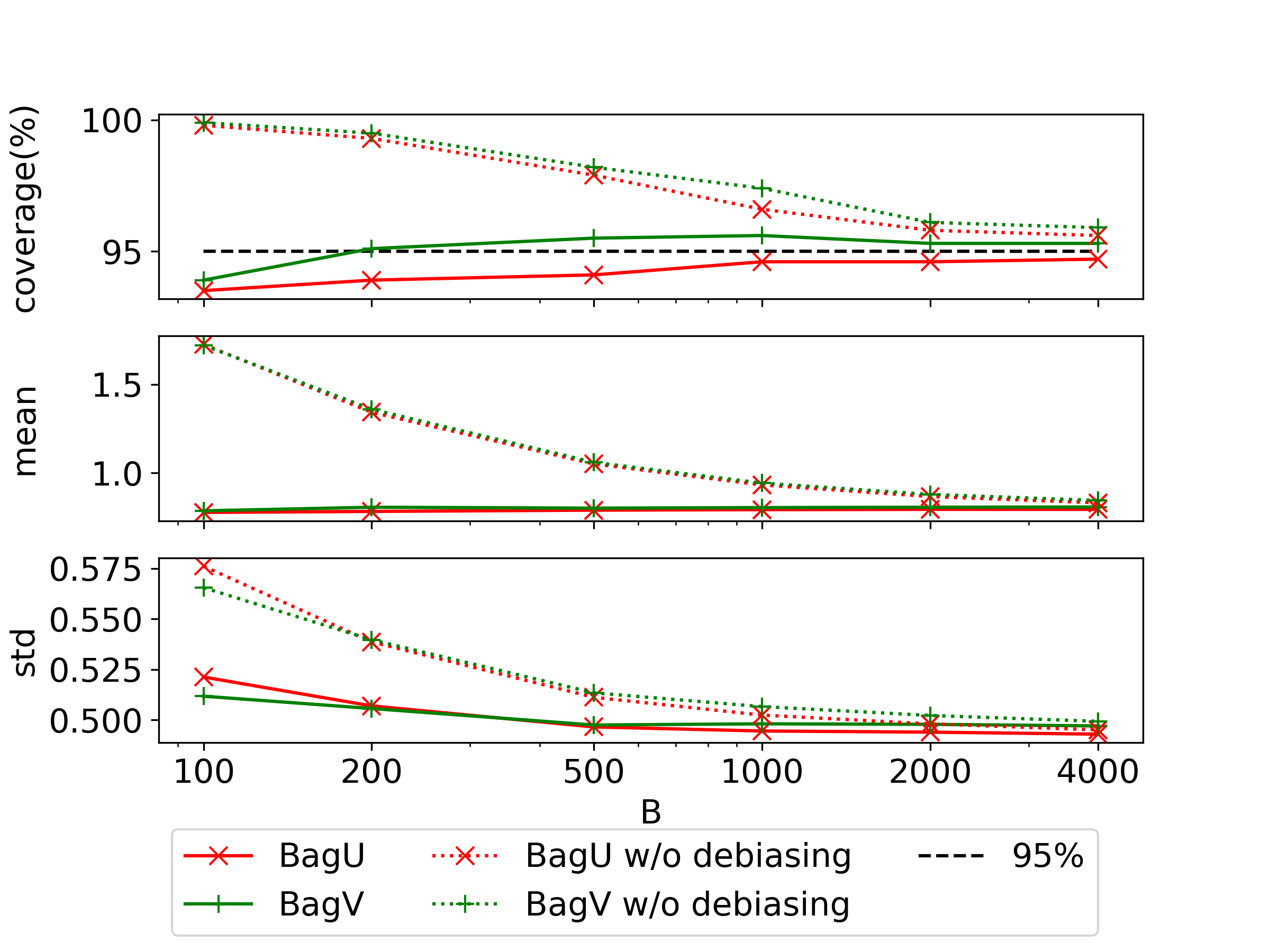
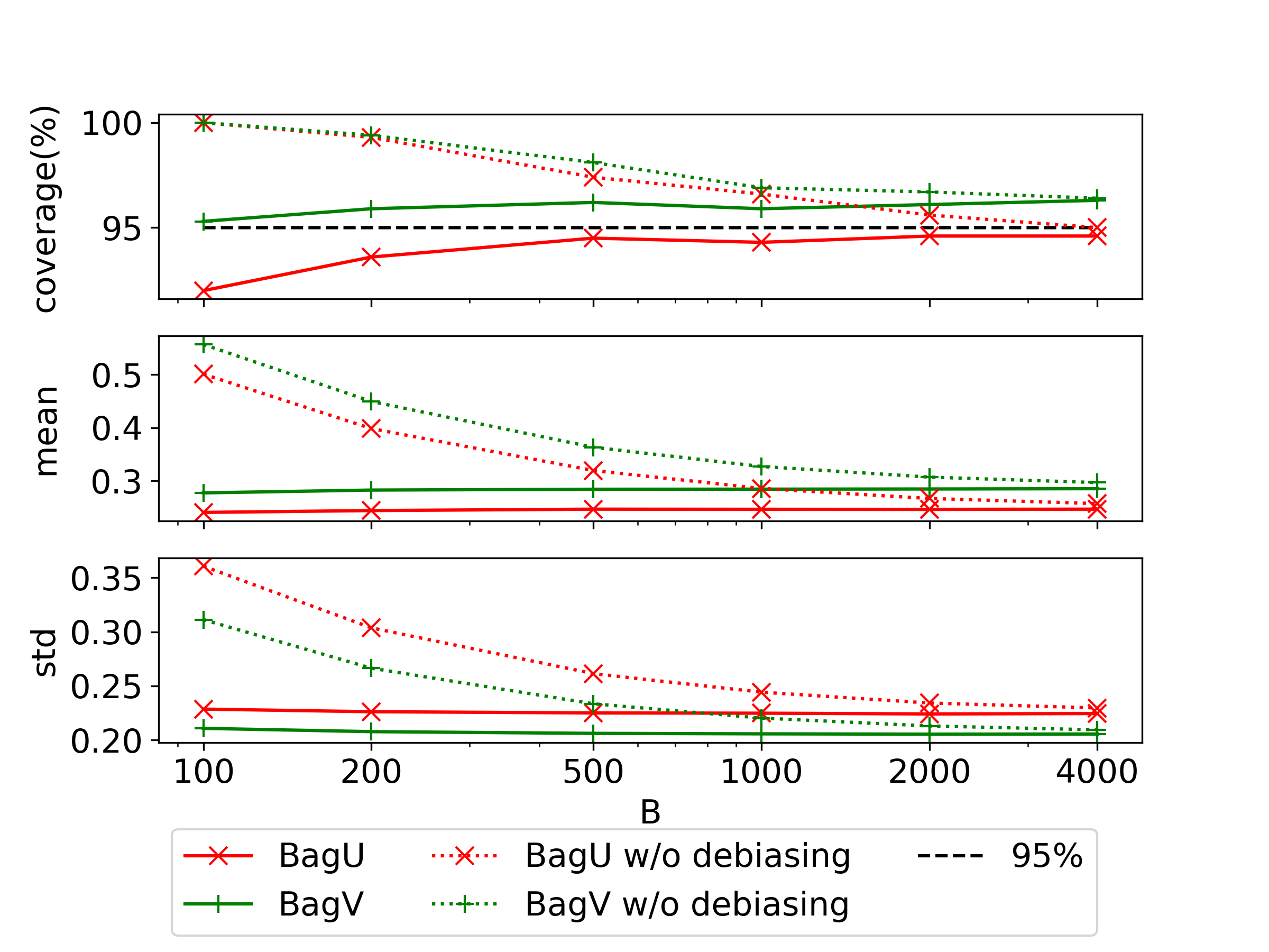
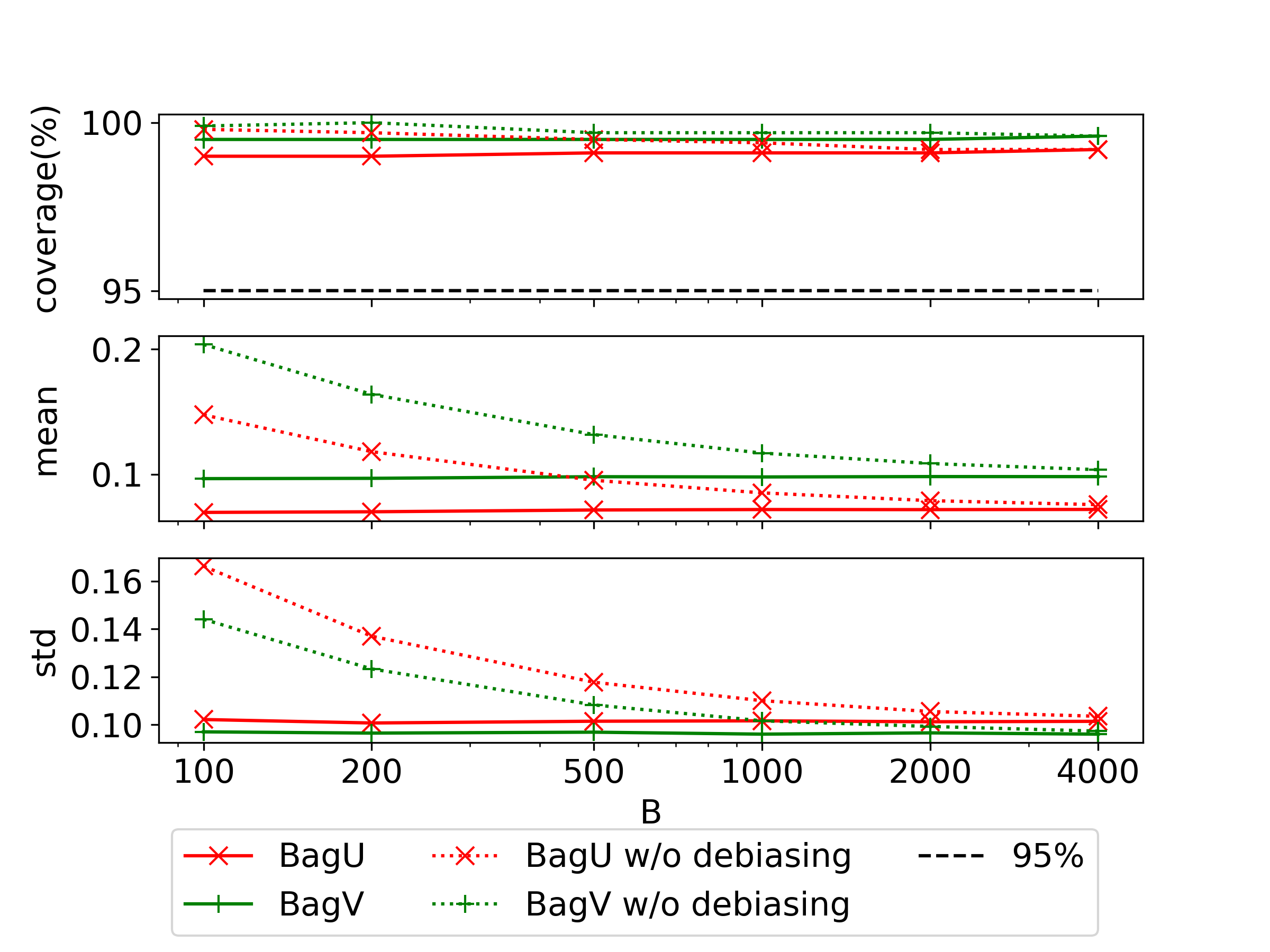
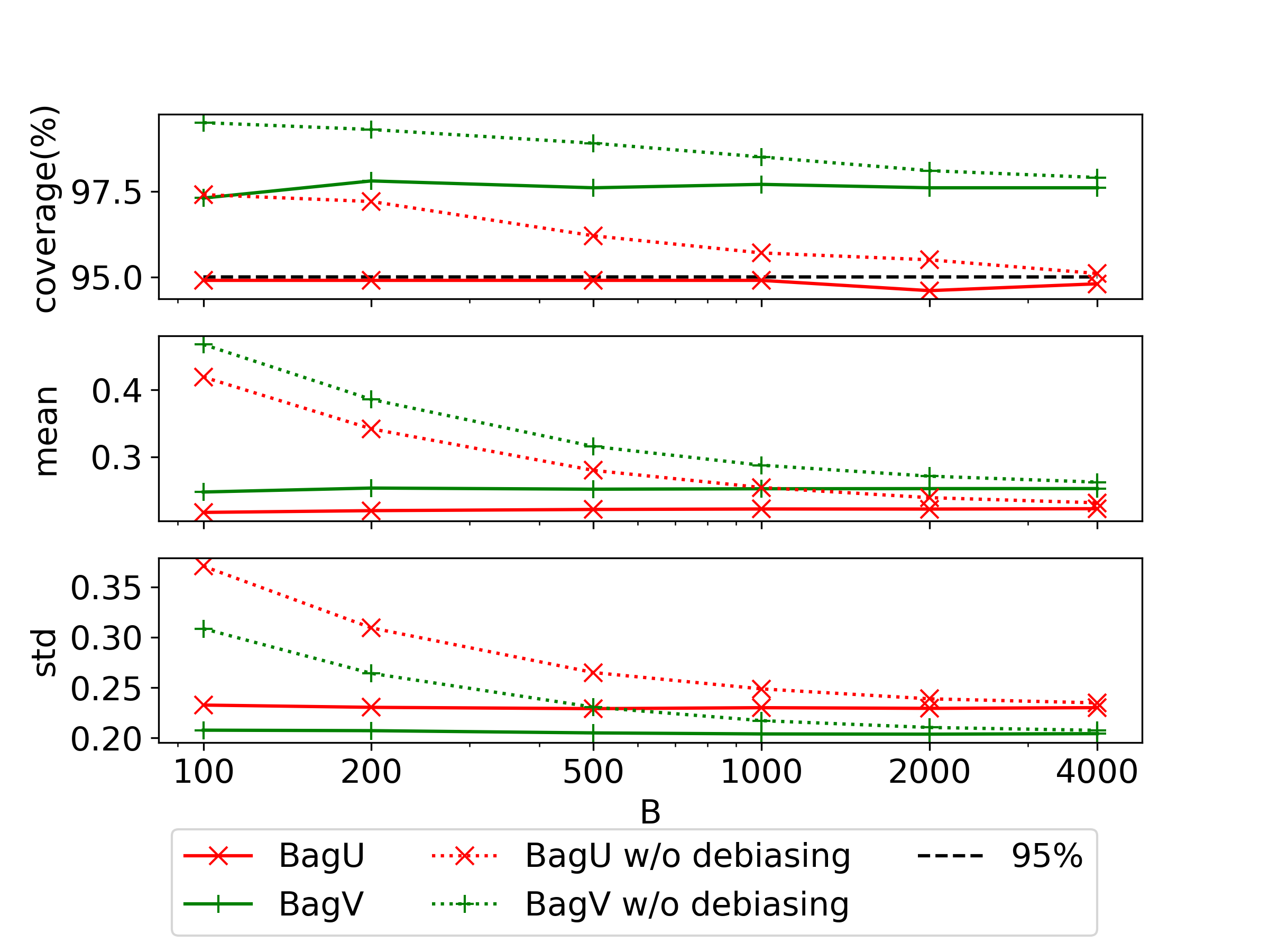
We simulate an i.i.d. data set of size , and use Algorithm 1 and its debiased variant Algorithm 2 to compute -level lower confidence bounds for the optimal value . To highlight the algorithmic difference, Algorithm 2 further subtracts from the IJ variance estimator a correction term for resampling with replacement, or for resampling without replacement, in order to remove the bias. We compare the performances of the two algorithms when the data size is fixed at , the resample size is fixed at , and the bootstrap size varies from a small size to , a sufficiently large size relative to as required by Theorem 6.3 for Algorithm 1.
Figure 1 shows the results on problems (23) and (24). Each plot in Figure 1 consists of three panels, where the top panel shows the estimated coverage probabilities of the constructed bounds based on independent runs and contains a dashed horizon line at the nominal level for benchmarking the coverage performance, the middle panel shows the mean of the bounds after being offset by the true optimal value (hence smaller values mean tighter bounds), and the bottom panel shows the standard deviation of the bounds across the runs. The legends “BagV w/o debiasing” and “BagU w/o debiasing” refer to Algorithm 1 with and without replacement respectively, whereas “BagV” and “BagU” refer to the counterparts of the debiased variant.
The results clearly show that both methods deliver bounds with correct coverage probabilities that are close to or higher than when the bootstrap size is relatively large (e.g., above ), and all the three metrics gradually converge as the Monte Carlo error diminishes when increases. However, the debiased variant, for both with and without replacement, seems to outperform Algorithm 1 in several ways under small and moderate bootstrap sizes. Firstly, the bounds generated with bias correction are tighter and less variable as evidenced by their smaller mean and standard deviation, and at the same time have less conservative and yet still accurate coverage probabilities around . This is consistent with the fact that the IJ variance estimator in Algorithm 1 is upward biased and may overestimate the true variance. Secondly, the performance of the debiased version is much less sensitive to the bootstrap size in the sense that the coverage, mean, and standard deviation of the bounds does not vary as drastically as Algorithm 1 under different bootstrap sizes. Based on the these observations, we recommend the debiased variant for general use of our bagging procedure. Comparing with and without replacement, we see that BagV has slightly higher coverages than BagU on both problems and generates slightly looser but less variable bounds for the linear program (24).
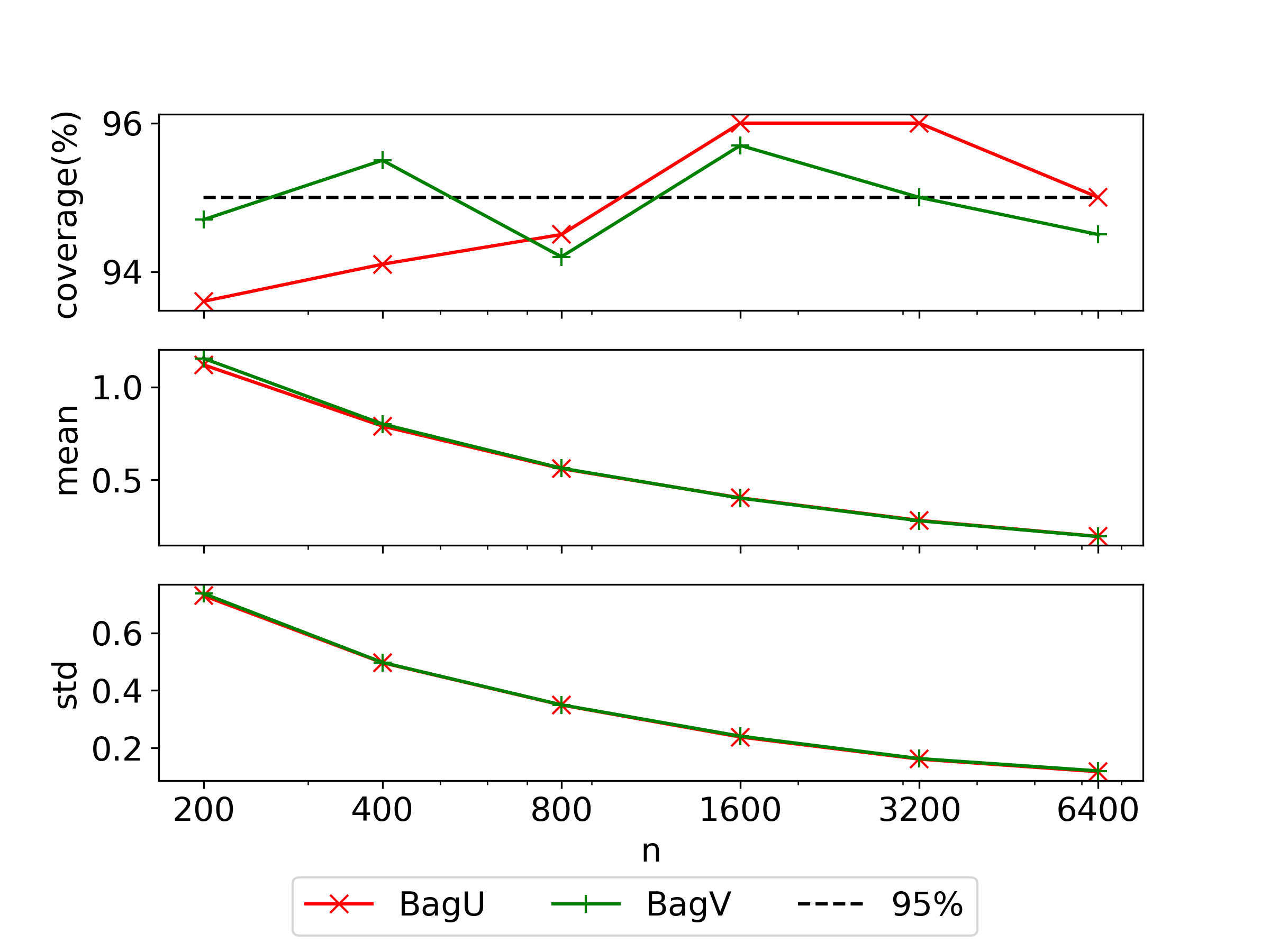
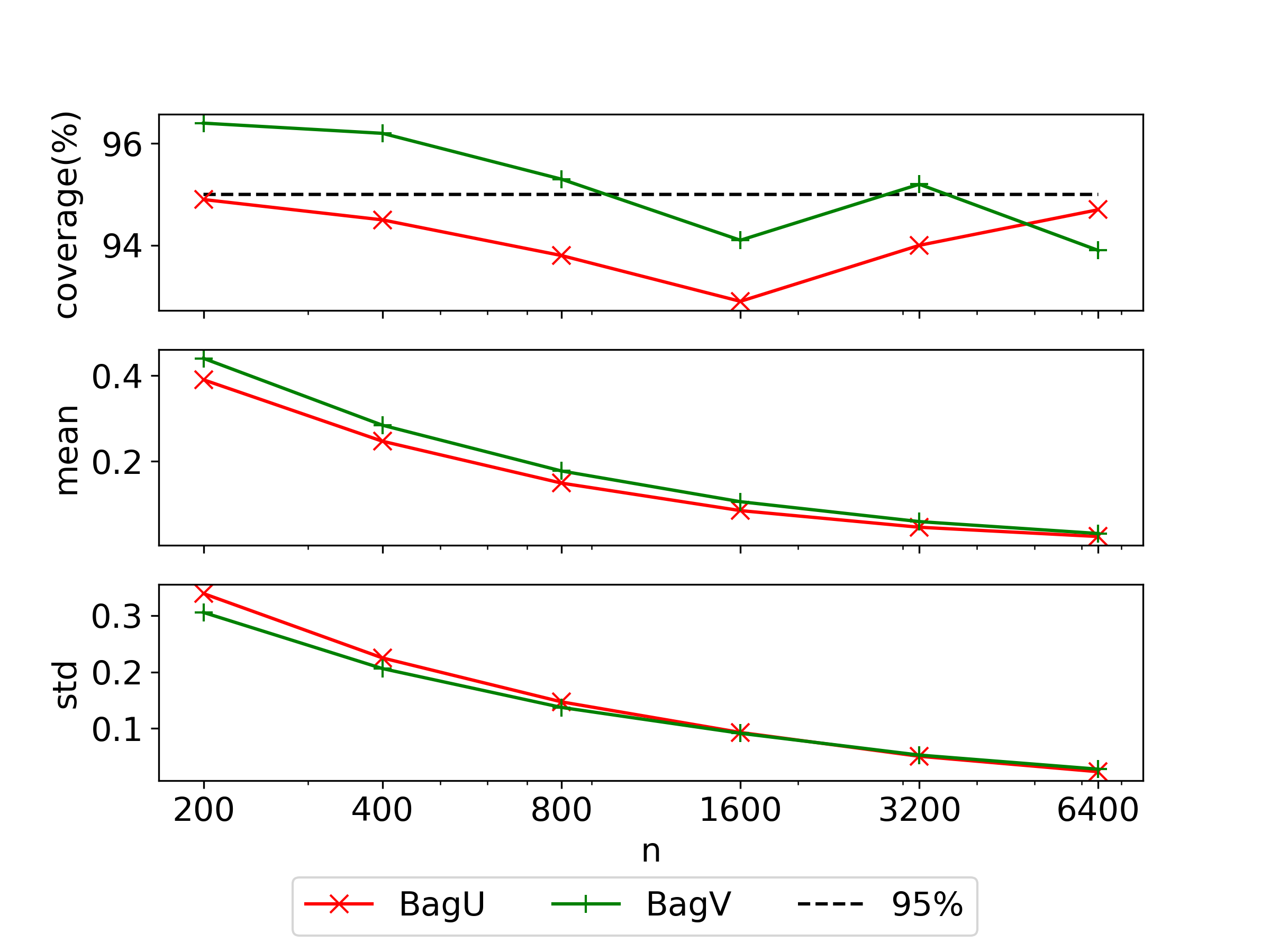
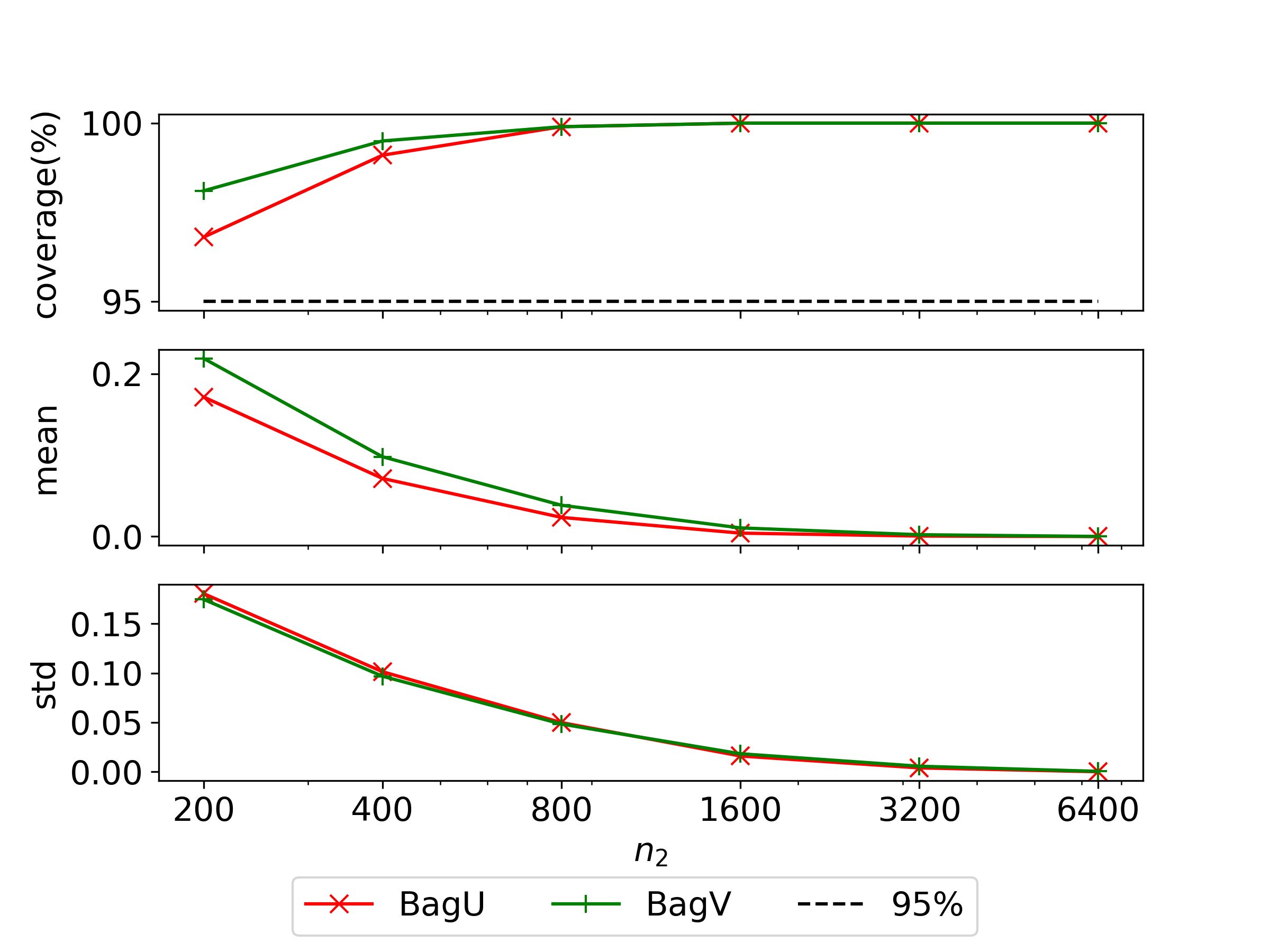
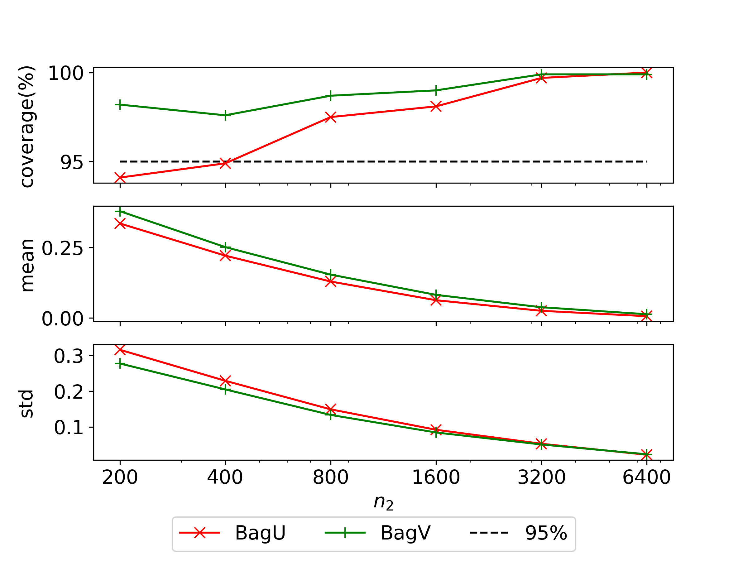
For the choice of the bootstrap size, Figure 1 suggests that is large enough for the debiased variant as further increasing it does not result in higher coverage accuracy or more stable bounds. To consolidate this choice, we test our debiased bagging procedure against increasing data sizes. Specifically, we fix , increase the data size from to , a much larger size than , and use a resample size . Figure 2 summarizes the results on the same two problems. Although in theory the bootstrap size is required to grow with the data size, the results show that for fixed the coverage probabilities are consistently close to across all data sizes, and that the bounds get tighter and more stable as the data size grows, which is in accordance with the tighter optimistic bound and the smaller variance of the bagging estimate. All these demonstrate that the required bootstrap size of our debiased variant depends lightly on the data size and that using delivers satisfactory performances for data sizes of high thousands. Throughout the rest of our experiments, the debiased variant with a fixed bootstrap size of will be used for our bagging procedures. Although not presented in the following subsections, our Algorithm 1 is found to perform similarly as the debiased variant if a larger bootstrap size that grows proportionally with the data size is used, e.g., . This can also be seen from Figure 1 where the results of the two procedures, whether with or without replacement, closely match under large bootstrap sizes. Lastly, the size admittedly could still be expensive for some problems. Further computation reduction is potentially achievable using recent cheap bootstrap approaches (Lam (2022a, b)); we leave the full investigation in this direction to future work.
8.2 Lower Bounds of Optimal Values
In this subsection we compare our bagging procedures with four other existing methods in computing -level lower confidence bounds for optimal values. For BatchP we use the critical value of -distribution with degrees of freedom when the number of batches , so as to enhance finite-sample performances as suggested in Mak et al. (1999), whereas in other methods the normal critical value is used in the standard error term of the bound.
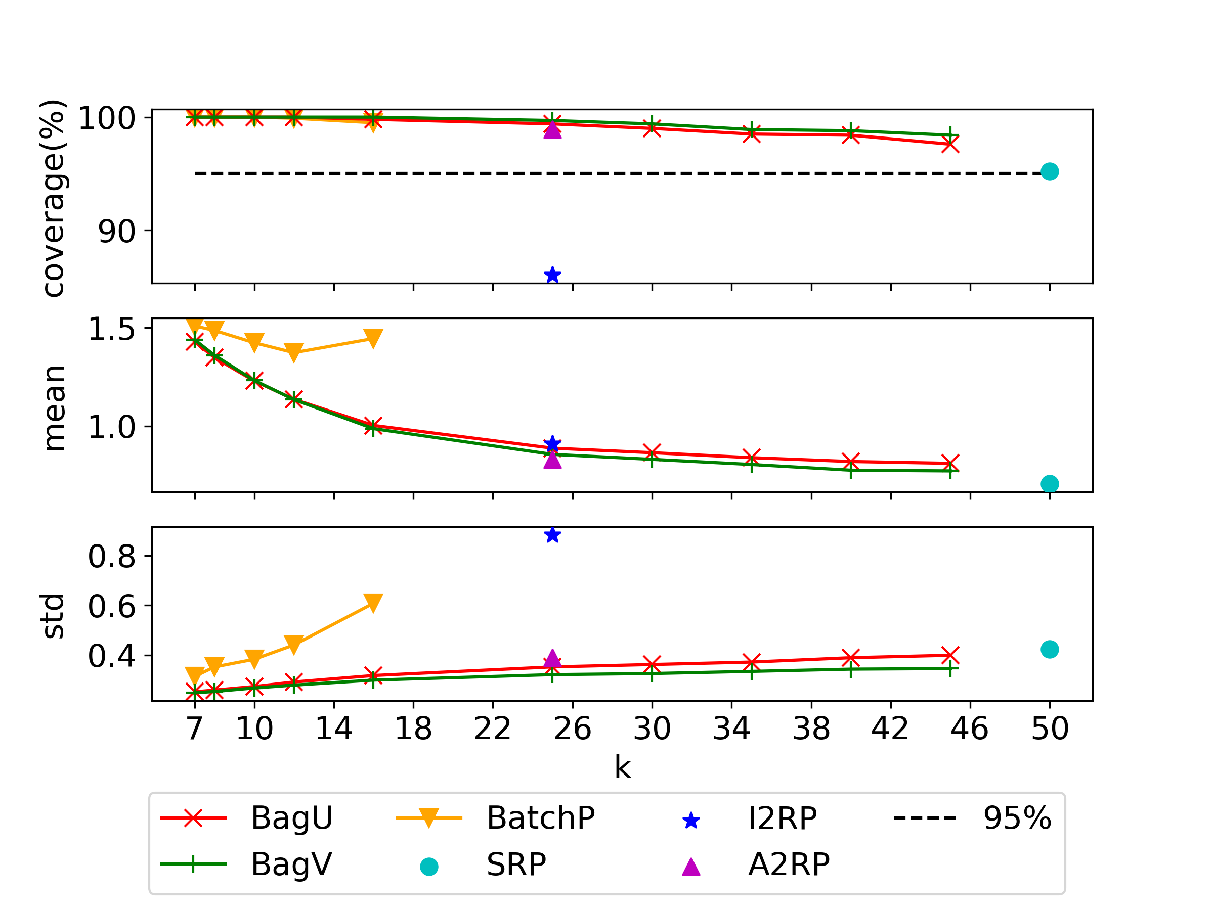
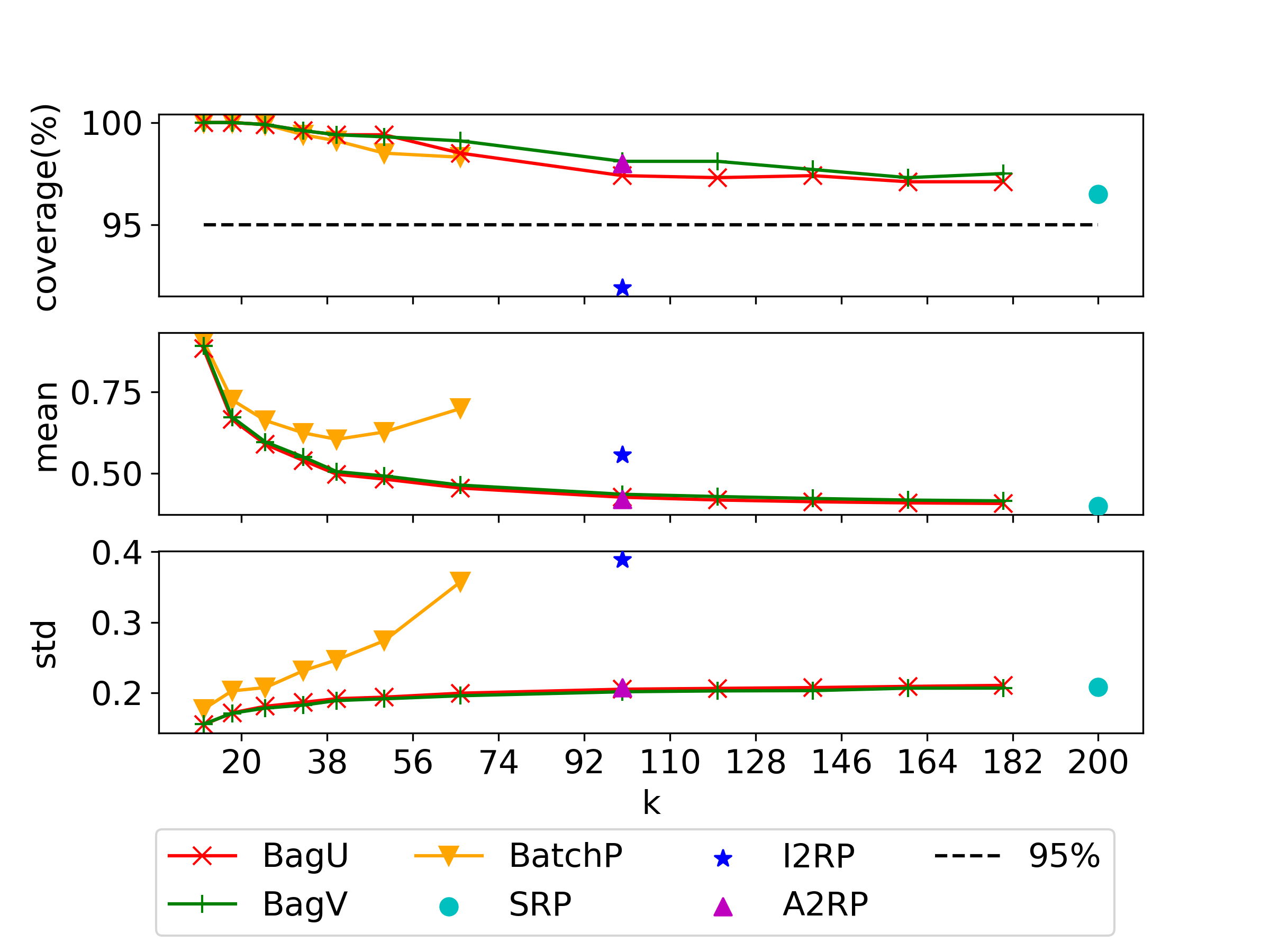
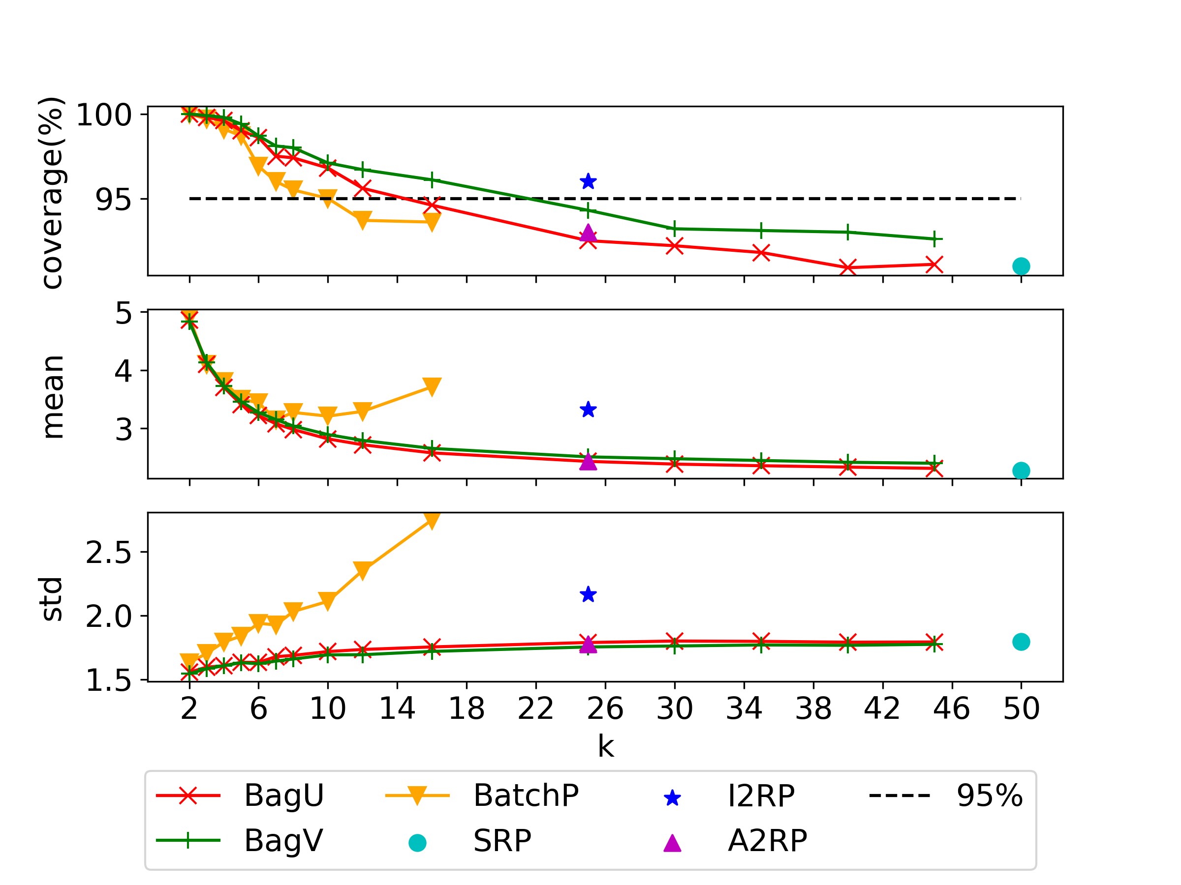
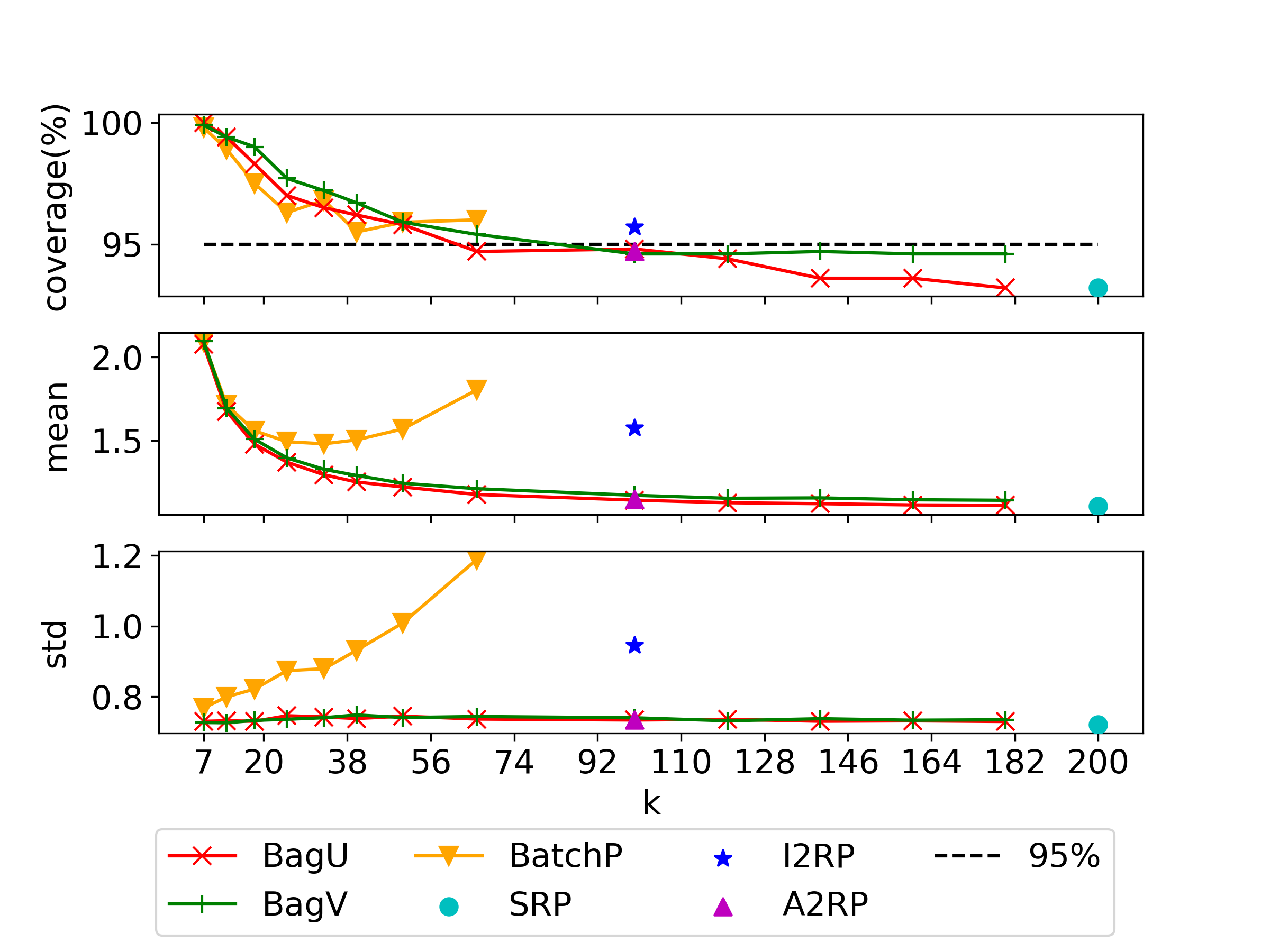
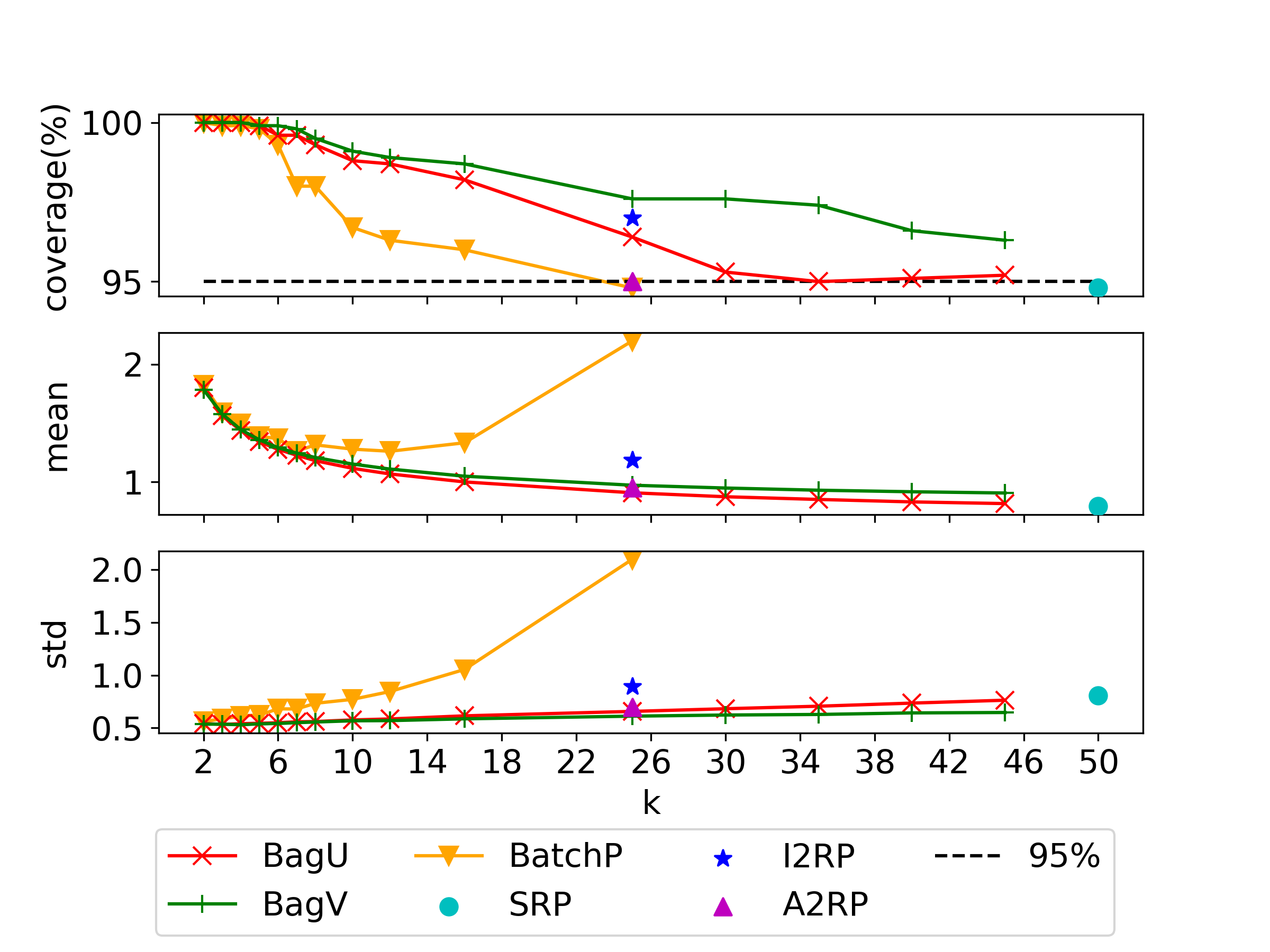
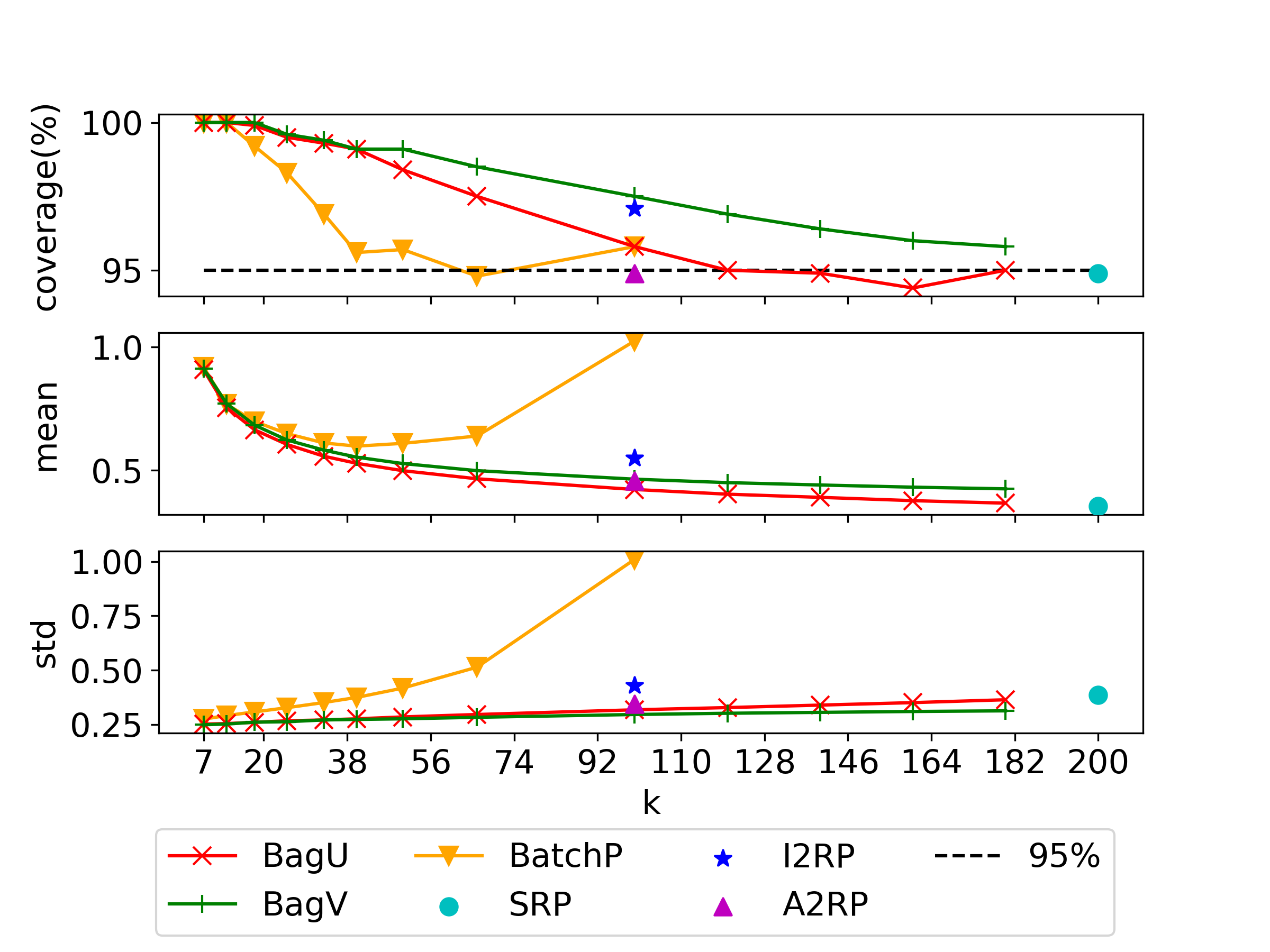
Figures 3, 4 and 5 summarize the results for problems (22), (23) and (24) respectively. Each figure contains two plots, one for data size and the other for , and each plot shows the estimated coverage probabilities, the mean and standard deviation of the bound after being offset by the optimal value (hence smaller values mean tighter bounds) under different batch sizes for BatchP or resample sizes for BagU and BagV, both denoted by . The SRP uses all the data to construct the SAA, hence its result corresponds to a point at , whereas I2RP and A2RP use half of the data to construct SAAs and their results are plotted at .
Figures 3 and 5 show that almost all the considered methods, over a wide range of resample sizes roughly from to of the data size for BagU and BagV, generate statistically valid bounds for problems (22) and (24) in the sense that the coverage probabilities are equal to or above the nominal value . The only exception is I2RP that undercovers for problem (22). Correspondingly, the I2RP bounds also have a high variability in this example. For problem (23), Figure 4 shows that BagU and BagV, as well as A2RP and SRP, undercover when the resample size is chosen large. However, BagV and A2RP undercover more mildly than BagU and SRP, e.g., the coverage is approximately for A2RP and BagV with close to and for BagU and SRP in Figure 4(a) when . This undercoverage is potentially due to the discrete nature of the integer program and gets improved as the data size grows from to .
Besides coverage, the considered methods differ in tightness and stability. We observe that BagU and BagV consistently output tighter (measured by the mean of the bound offset by the optimal value) and more stable (measured by the standard deviation) bounds than BatchP when the batch size in BatchP and the resample size in bagging are set the same. This difference in tightness and stability becomes more noticeable as increases. Compared to direct-CLT bounds, our bagging bounds also appear tighter and more stable than I2RP (either when the resample size or is close to ) on all three problems, whereas A2RP and SRP bounds are similarly tight and stable as our bagging bounds in all the cases.
Figures 3-5 also show the tradeoff between tightness and statistical accuracy in BatchP and how it is improved by bagging. The monotonicity relation between the batch size and the optimistic bound entails that the bound should become tighter as increases. However, the bound by BatchP gets tighter at first under relatively small batch sizes but then becomes looser instead as the size further increases. This non-monotonic behavior appears since, as the batch size gets large, too few batches are available for the procedure to maintain the desired coverage accuracy. To mitigate this issue, we resort to using critical value in place of the normal one which loosens the bound in exchange for better coverages. Such a tradeoff is significantly improved in our bagging procedures due to the many resampled SAAs, as evidenced by the monotonically improving tightness and accurate coverages of the bounds across a wide range of resample sizes.
To summarize, for bounding optimal values our bagging bounds are generally as competitive as A2RP and SRP and outperform BatchP and I2RP in terms of coverage, tightness and stability, whereas between the two bagging bounds BagV exhibits a more reliable coverage performance than BagU while performing similarly in tightness and stability. Our next experiment on bounding optimality gaps will further reveal the performance differences among bagging bounds, A2RP and SRP.
8.3 Upper Bounds of Optimality Gaps
Now we test our methods in bounding optimality gaps of solutions. We first solve the SAA formed by data points to obtain a solution , then generate independent data points . These (and possibly the first data points as well) are then used to compute an upper confidence bound for the optimality gap . For convenience we denote as the total sample size.
We consider two approaches to bounding the gap, one reusing the first data points, and the other not. The first approach is to use the Bonferroni Correction (BC). Specifically, we use the second group of data to compute as a upper confidence bound of , where are the sample mean and variance of , and compute a lower confidence bound of the true optimal value using all the data as in the previous section. By BC we know
so that if and are both asymptotically at least , then is an asymptotically valid confidence bound for the gap .
The second approach is a Common Random Numbers (CRN) variance-reduction technique proposed by Mak et al. (1999). This approach generates upper bounds of the gap via computing lower bounds for the optimal value of the modified objective where is viewed as fixed. Specifically, given we use the second group of data to compute a lower confidence bound for this new objective, and then negate the lower bound to obtain a valid upper bound for .
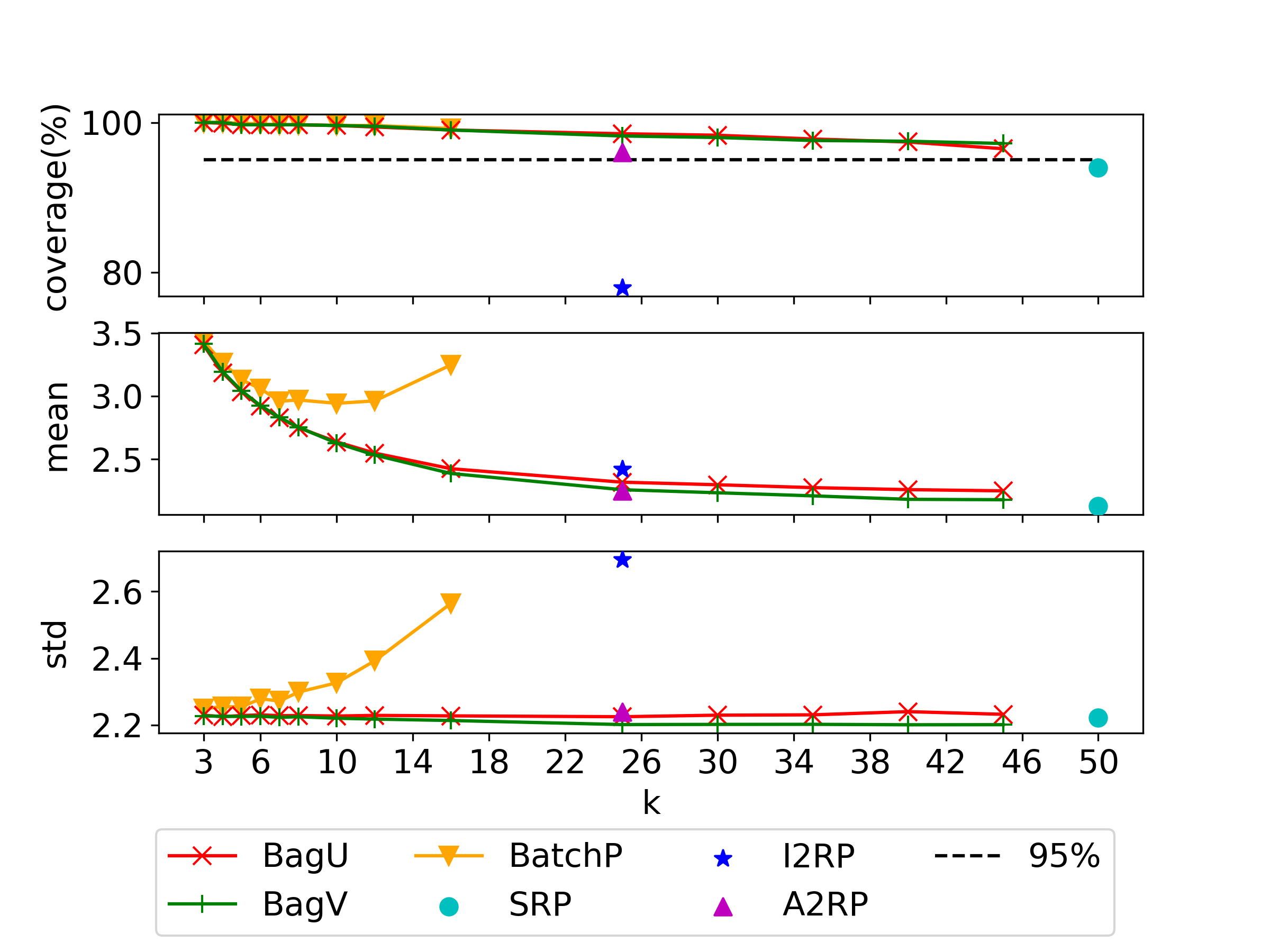
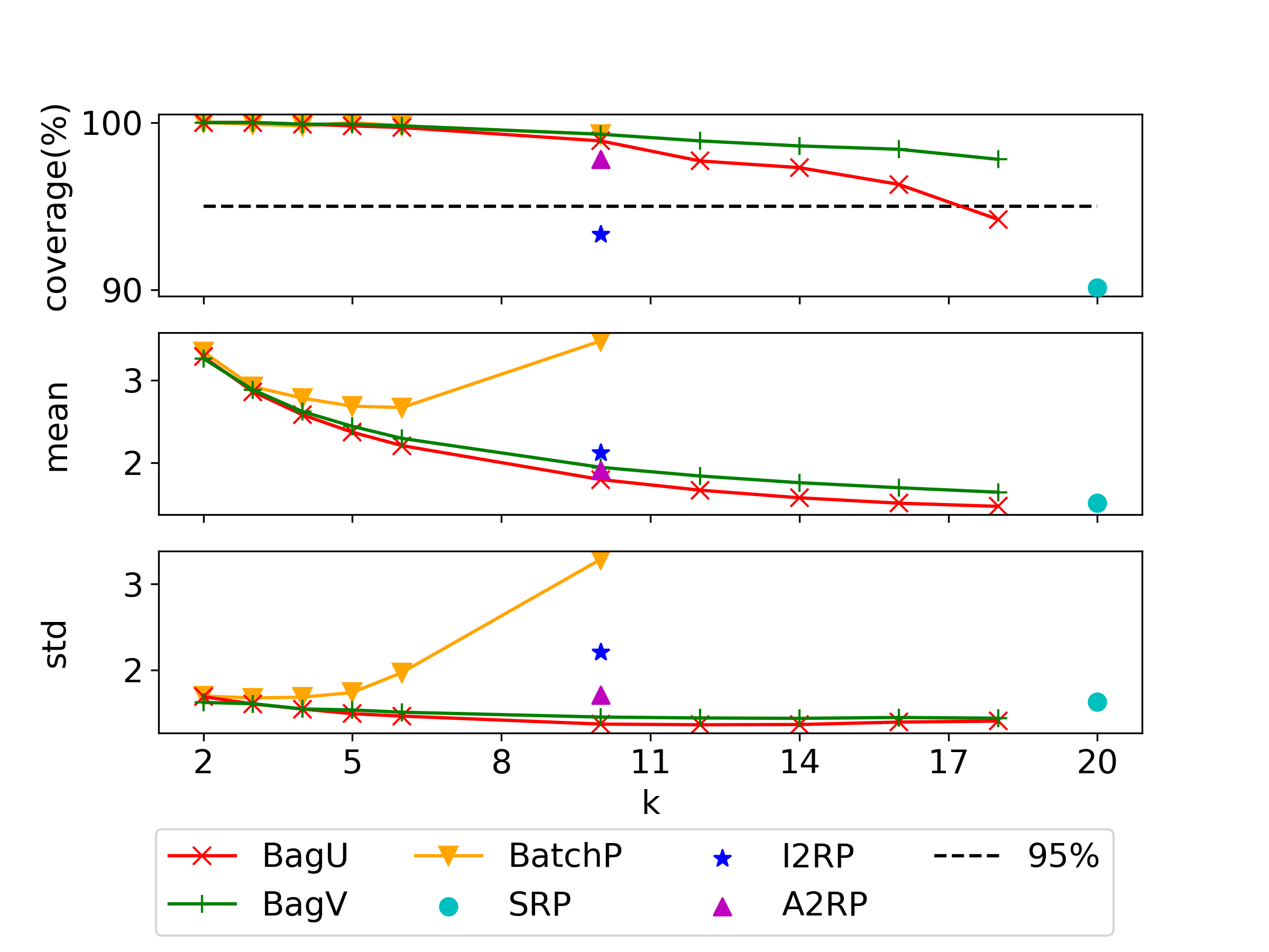
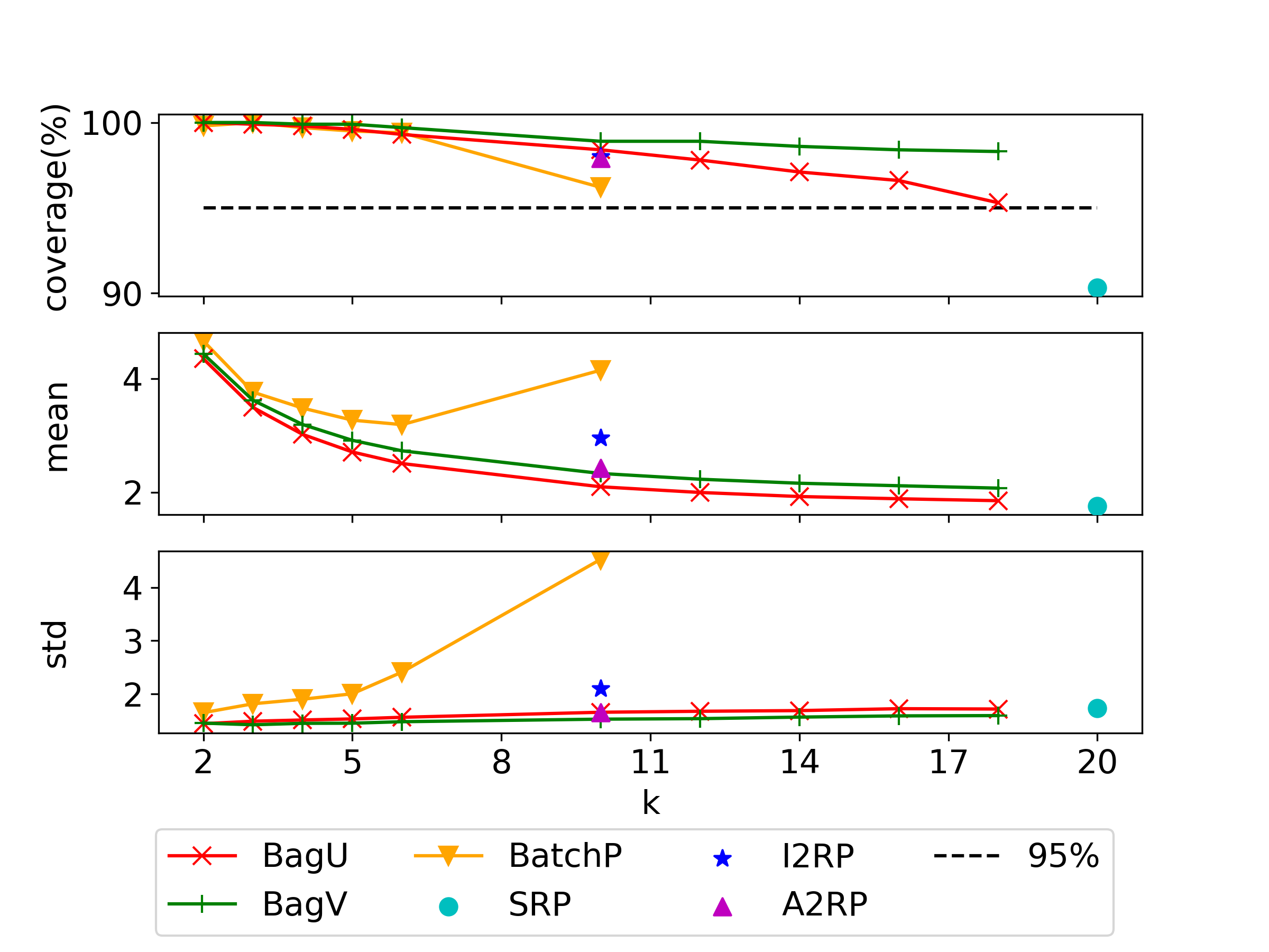
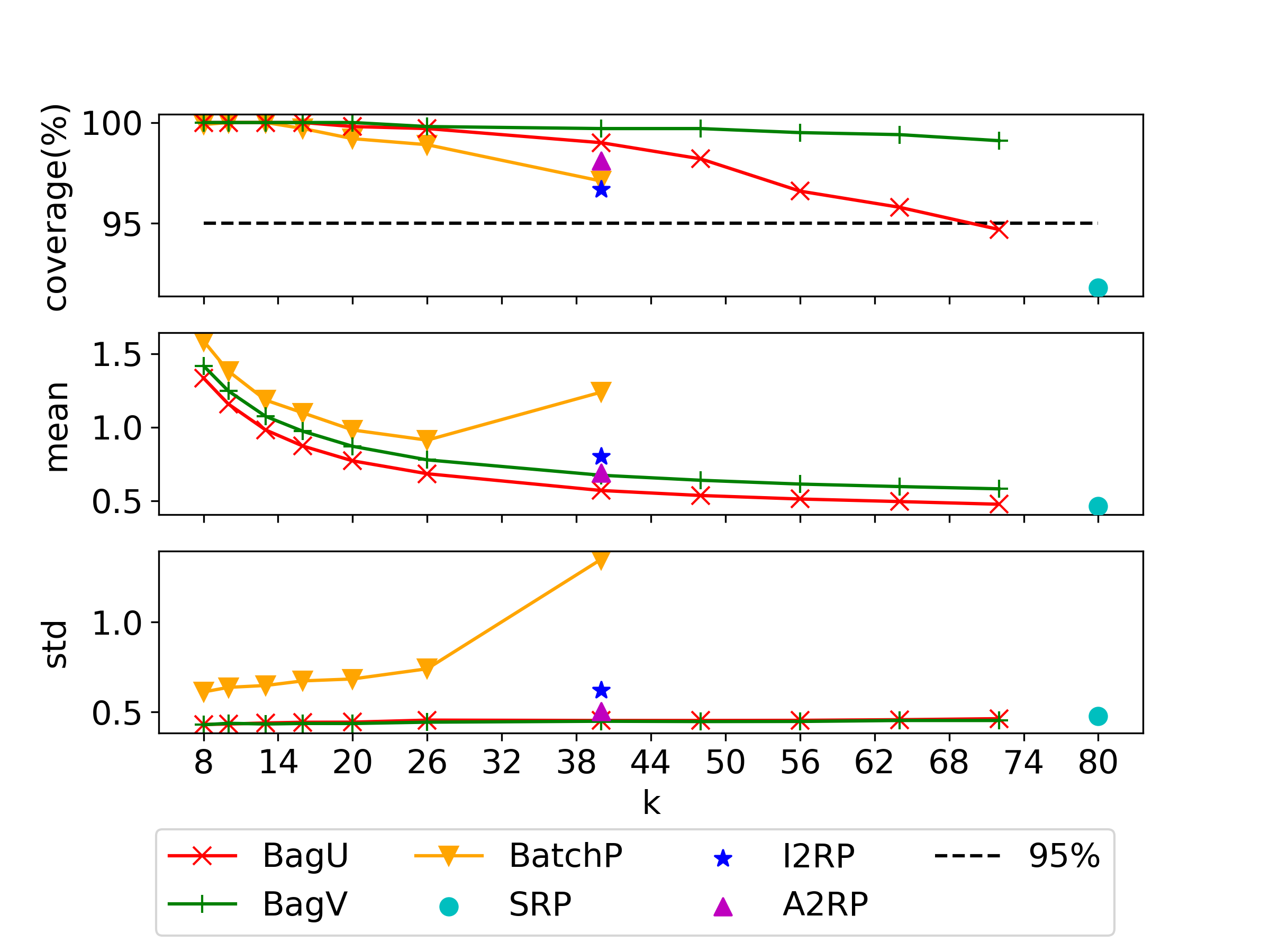
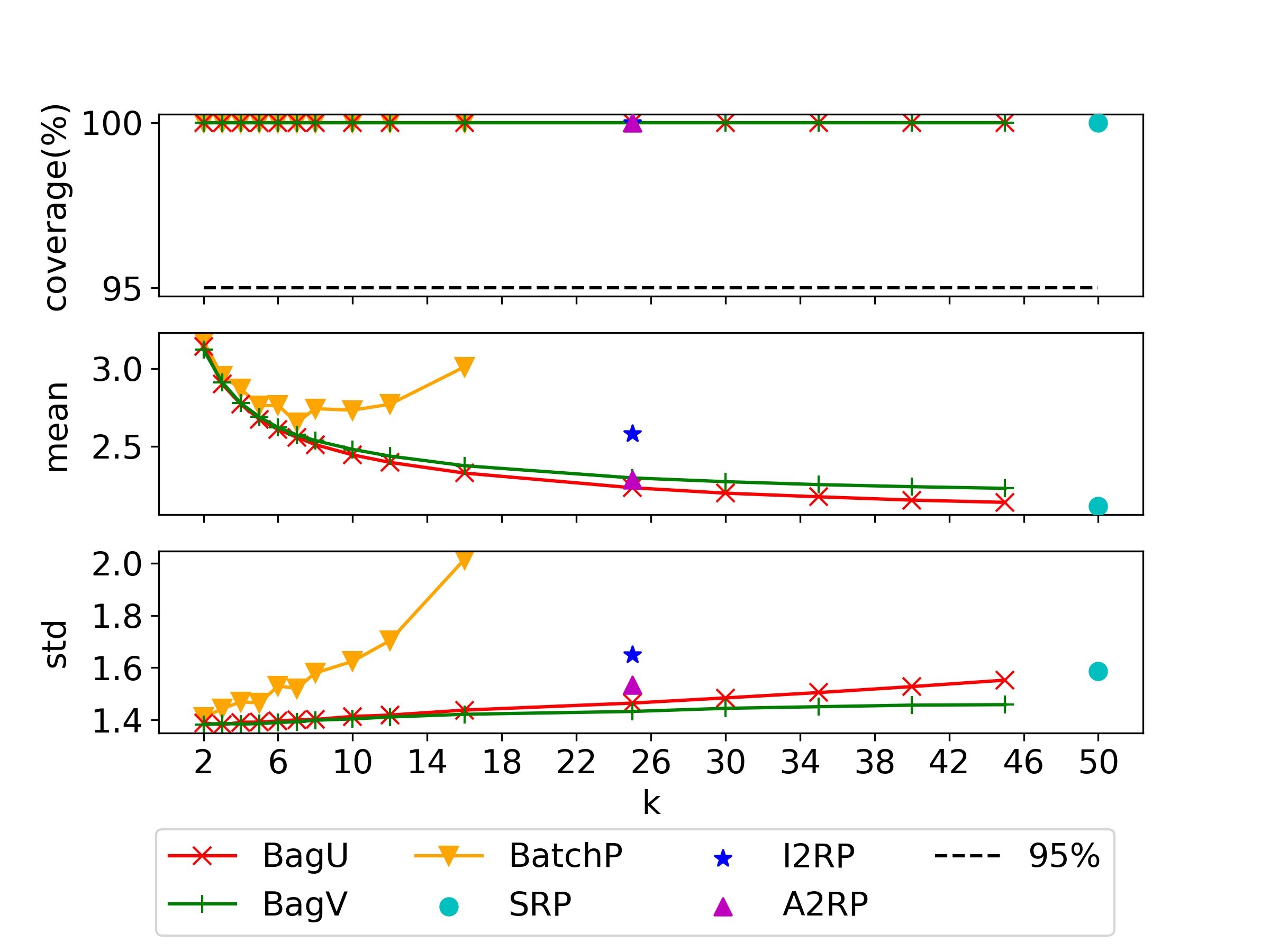
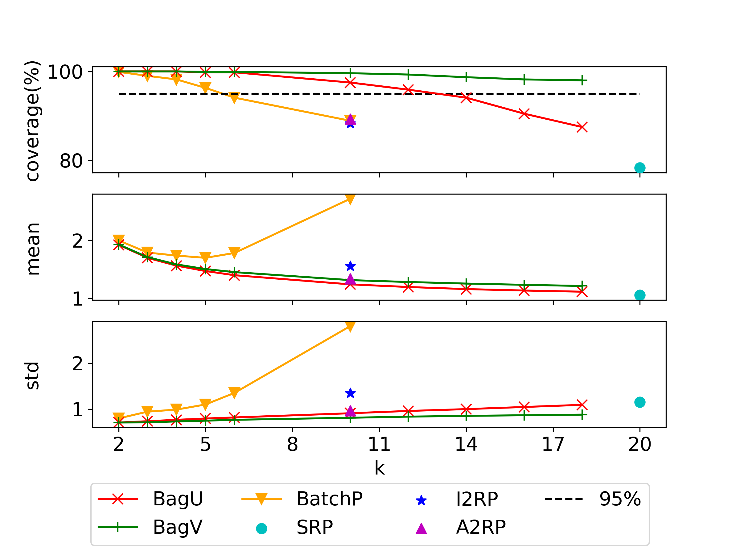
Figures 6, 7 and 8 summarize the results for problems (22), (23) and (24) respectively in a similar fashion as in Section 8.2. Each plot in these figures shows again the estimated coverage probabilities, the mean and the standard deviation of the upper bounds across independent runs. In each experiment, whether BC or CRN, the data set is split into and , i.e., and for each total size .
We see a few similar observations as in Section 8.2. The two bagging procedures generate statistically valid upper bounds in almost all the cases. The only exception is Figure (8(b)) where all methods but BagV undercovers for problem (24) under relatively large resample sizes. BatchP also possesses the desired coverage probability in most cases, but the generated bounds are looser and less stable than those by other methods. In particular, when the CRN approach is used (i.e., Figures 6(b), 7 and 8(b)) the tightest bound by BatchP across different batch sizes can be twice of that by BagU and BagV. For direct-CLT bounds, A2RP continues to exhibit competitive performances on all the three problems except that in Figure 8(b) it undercovers on problem (24) whereas BagV still maintains an accurate coverage with similar tightness and stability as A2RP when is chosen close to . In the same example BagU also has an accurate coverage for resample sizes around but starts to undercover like A2RP when further approaches . Compared to I2RP, our bagging bounds continue to generate tighter and stabler bounds in all cases and sometimes have more accurate coverages (Figure 6).
Some new observations are as follows. First, we see that SRP suffers from severe undercoverage issues (e.g., under in Figure 8(b)) on all the three problems when the CRN approach is adopted. We comment that this undercoverage of SRP with CRN is not a coincidence as the objective variance used in SRP tends to frequently underestimate the true variance if the candidate solution to bound the gap for is obtained from an SAA. To explain, when is also generated from an SAA then it is expected to have a similar distribution as the the solution obtained from the SAA formed by the second portion of data in the CRN approach, and therefore if lies in a high-density area of this distribution, which is likely to happen, then can very well be closer to (or even exactly in the case of discrete decision space) than to the true optimal solution , in which case the objective variance used in SRP becomes significantly smaller than the true variance on a relative scale. This has also been observed and discussed in length in Bayraksan and Morton (2006) where a strategy that uses a suboptimal SAA solution in place of the exact solution is proposed to reduce the chance of the two solutions being close. A2RP and I2RP can also mitigate this issue by using two instead of one SAA solution, whereas our bagging procedures push this further by estimating the variance using many resampled SAA solutions. As evidenced in Figures 6, 7 and 8, A2RP and our bagging bounds have significantly more accurate coverages than SRP, and in particular BagV is the only method that has a correct coverage in Figure 8(b) and also appears tighter and stabler than A2RP when the resample size is set close to the full data size.
Second, we observe that the coverage of BagV is less sensitive to the resample size than BagU, and that when SRP undercovers (e.g., Figures 6(b), 7 and 8(b)) the coverage of BagU starts to resemble that of SRP while BagV does not as the resample size approaches the full data size. This reveals that in practice a larger resample size can be used with BagV than with BagU in maintaining an accurate coverage. The resemblance between BagU and SRP under large and the robust coverage of BagV can be explained based on the amount of variability brought by different resampling methods. To explain, for resampling with replacement the variability (standard deviation) of the resampled SAA objective decays at a canonical rate as the resample size grows towards since the sampling is i.i.d. and uniform over the data, whereas for resampling without replacement the variability can be calculated to decay at the rate which behaves like for moderate but decays more quickly as for close to . In other words, when is close to the resampled SAAs and their optimal solutions in BagU are significantly more similar to the original full SAA than those in BagV, and therefore BagU resembles SRP while BagV still has stable and accurate coverages. Although our theory does not directly capture these phenomena, the smaller resampling variability of BagU can be hinted by its additional factor in the IJ variance estimator in Algorithm 1 that compensates for the variability of BagU under large resample sizes in order to match the correct magnitude of the variance. In light of this key difference between BagU and BagV, we recommend that the resample size should be no larger than for BagU in limited-data situations.
Third, in general the CRN approach generates tighter and stabler confidence bounds than the BC approach thanks to variance reduction. In particular, Figures 6 and 8 shows that with the same split of the data, the bounds by CRN can be up to twice tighter than those by BC as measured by the mean of the generated bounds, and the standard deviation of the bounds can be reduced by up to as can be seen from Figure 8. We also observe that the BC approach tends to overcover the optimality gap, potentially because of the looseness of the union bound.
8.4 Variance Reduction for Problems with Multiple Optima
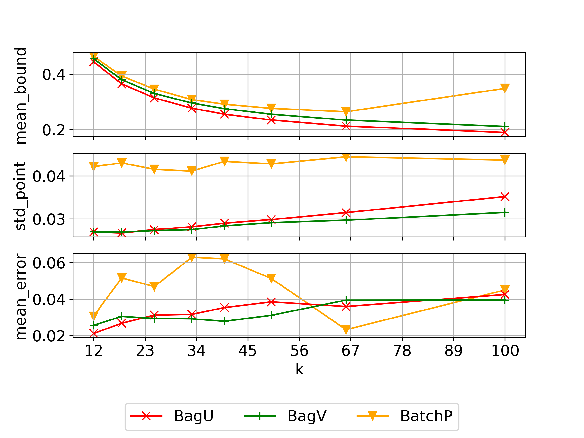
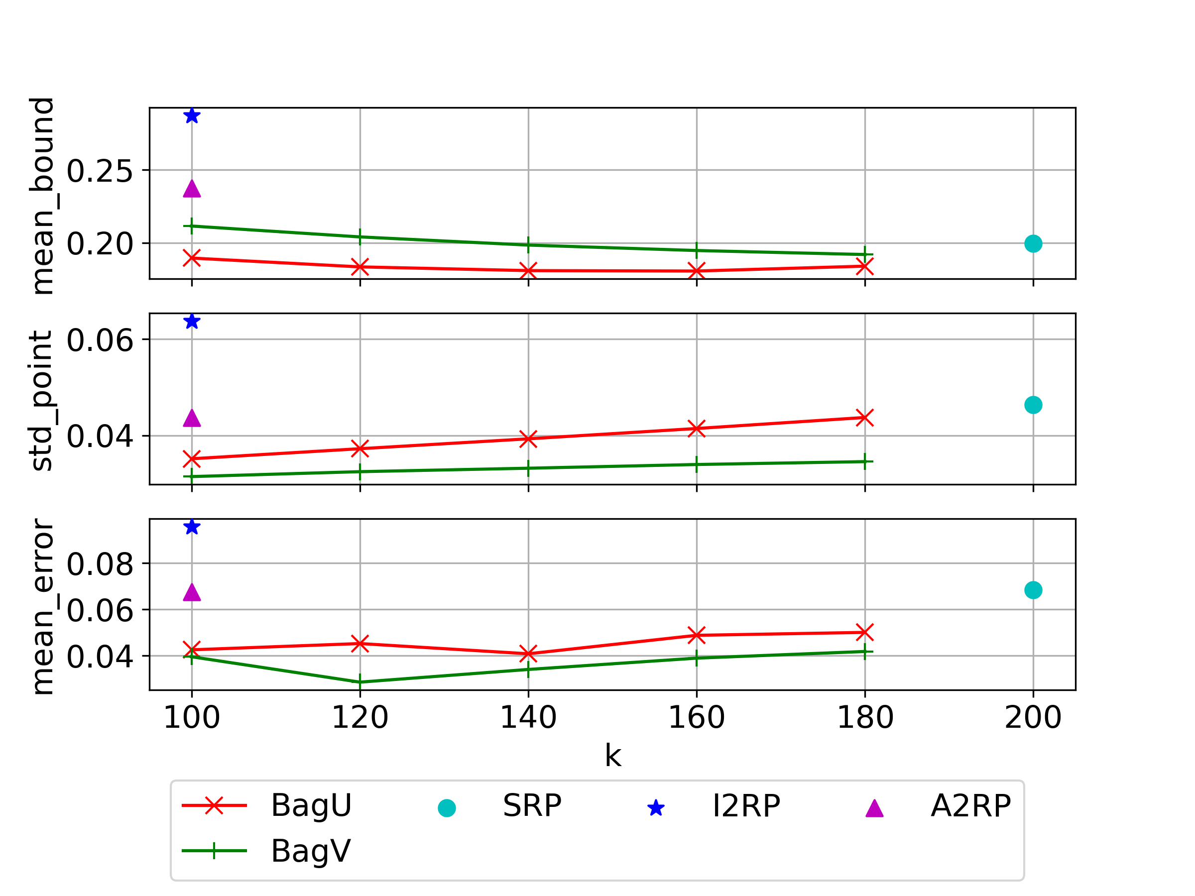
Our theory suggests that when there are multiple optimal solutions the bagging estimate has a smaller variance than both BatchP and direct-CLT estimates, and in this subsection we compare the variances of these estimates using problem (25). We set the data size , and compute lower confidence bounds for the optimal value using different resample sizes for bagging or batch sizes for BatchP. Results are summarized in Figure 9, where the the top panel of each plot shows the mean of the bound (offset by the true optimal value) under different batch sizes or resample sizes, the middle panel plots the standard deviation of the point estimate of each bound, and the bottom panel shows the average standard error estimate in each bound. The coverage probabilities of all the methods are above and hence omitted from the plots.
The standard deviation of our bagging point estimates are consistently smaller than that of the BatchP point estimate ( versus ) regardless of the choice for the batch size or the resample size , as shown in Figure 9(a). Compared to SRP, A2RP and I2RP, Figure 9(b) also shows consistently smaller standard deviations from our bagging point estimates (especially BagV). The larger standard deviation of the I2RP estimate is expected since its point estimate uses only half of the data. All these are aligned with the variance reduction benefit of bagging as described in Theorem 7.2. Besides variance of the point estimates, the mean standard error term in our bagging bounds are also smaller than that of SRP, I2RP, and A2RP ( versus ) and BatchP at most choices of . This again verifies the reduced variance of our bagging point estimates. Comparing BagU and BagV, we see that the BagV bound has a slightly smaller variance in the point estimate and also a smaller standard error term than BagU, but the overall bound is slightly looser. This relative looseness of BagV is consistent with our theory that the BagU point estimate is unbiased with respect to the optimistic bound of the optimal value whereas BagV is downward biased.
8.5 Summary and Recommendation
We summarize our experimental findings. Our bagging bounds, especially BagV, in general appear as competitive as existing methods in terms of coverage attainment, tightness and stability, while outperform them in different specific cases. More precisely, compared to BatchP, our bagging bounds are significantly tighter and stabler in almost all cases thanks to the improved tradeoff between tightness and statistical accuracy. Compared to direct-CLT bounds, BagU and BagV have more accurate coverages than I2RP (Figures 3, 6, 8(b)) and SRP (Figures 4, 7 and 8(b)) especially when bounding optimality gaps, and generate tighter and stabler bounds than I2RP in all the cases. A2RP shows similarly competitive performances as bagging methods in almost all the cases, but our BagV with a resample size close to the data size appears to have more accurate coverages on problem (24) (Figure 8(b)), generates stabler bounds in some cases (Figures 6(b) and 8(a)), and in general is slightly tighter (e.g., Figure 3(a), 6, 7 and 8(b)). In the case of multiple optima, our bagging bounds are tighter than all existing bounds (Figure 9) when the resample size is chosen close to the data size.
For algorithmic configurations of our bagging procedures, we recommend the debiased variant (Algorithm 2) with a fixed bootstrap size for higher accuracy in the IJ variance estimate. The resample size can be chosen close to the data size for BagV to generate tight bounds, but no larger than of the data size for BagU under limited data to prevent its behavior mimicking SRP and maintain an accurate coverage.
Regarding the choice between BagU and BagV, we note that BagU generates slightly tighter bounds than BagU in most cases except Figures 3(a) and 6(a) due to the downward bias of . However, bounds by BagV have slightly smaller standard deviations than those by BagU, and BagV’s coverage performance is less correlated with that of SRP under large resample sizes due to the larger variability in the resampled SAA than BagU as explained in Section 8.3, making BagV less prone to coverage issues. In fact, the only case that BagV has minor undercoverage is Figure 4(a) where BagU undercovers more severely. From these observations, we recommend BagV based on its superior stability and safer coverage attainment, despite its slight looseness compared to BagU. However, if bound tightness is of importance, then BagU could be preferred. On a final note, results presented in this section are a representative part of our experiments, and additional results can be found in Appendix 16.
We gratefully acknowledge support from the National Science Foundation under grants CMMI-1542020, CMMI-1523453 and CAREER CMMI-1653339/1834710. We thank David Morton and David Woodruff for the greatly helpful suggestions and communications on this work. A preliminary conference version of this work, Lam and Qian (2018), has appeared in the Proceedings of the Winter Simulation Conference 2018.
References
- Bayraksan and Morton (2006) Bayraksan G, Morton DP (2006) Assessing solution quality in stochastic programs. Mathematical Programming 108(2-3):495–514.
- Bayraksan and Morton (2011) Bayraksan G, Morton DP (2011) A sequential sampling procedure for stochastic programming. Operations Research 59(4):898–913.
- Ben-Tal et al. (2013) Ben-Tal A, Den Hertog D, De Waegenaere A, Melenberg B, Rennen G (2013) Robust solutions of optimization problems affected by uncertain probabilities. Management Science 59(2):341–357.
- Bertsimas et al. (2018) Bertsimas D, Gupta V, Kallus N (2018) Robust sample average approximation. Mathematical Programming 171(1-2):217–282.
- Birge and Louveaux (2011) Birge JR, Louveaux F (2011) Introduction to Stochastic Programming (Springer Science & Business Media).
- Blanchet et al. (2019) Blanchet J, Kang Y, Murthy K (2019) Robust wasserstein profile inference and applications to machine learning. Journal of Applied Probability 56(3):830–857.
- Blom (1976) Blom G (1976) Some properties of incomplete U-statistics. Biometrika 63(3):573–580.
- Borkar (2009) Borkar VS (2009) Stochastic Approximation: A Dynamical Systems Viewpoint, volume 48 (Springer).
- Breiman (1996) Breiman L (1996) Bagging predictors. Machine learning 24(2):123–140.
- Calafiore (2017) Calafiore GC (2017) Repetitive scenario design. IEEE Transactions on Automatic Control 62(3):1125–1137.
- Carè et al. (2014) Carè A, Garatti S, Campi MC (2014) FAST – Fast algorithm for the scenario technique. Operations Research 62(3):662–671.
- Chen and Lopes (2020) Chen JX, Lopes M (2020) Estimating the error of randomized newton methods: A bootstrap approach. International Conference on Machine Learning, 1649–1659 (PMLR).
- Chen and Woodruff (2022) Chen X, Woodruff DL (2022) Software for data-based stochastic programming using bootstrap estimation. Optimization-online.org .
- De la Pena and Giné (2012) De la Pena V, Giné E (2012) Decoupling: From Dependence to Independence (Springer Science & Business Media).
- Delage and Ye (2010) Delage E, Ye Y (2010) Distributionally robust optimization under moment uncertainty with application to data-driven problems. Operations Research 58(3):595–612.
- Dentcheva et al. (2017) Dentcheva D, Penev S, Ruszczyński A (2017) Statistical estimation of composite risk functionals and risk optimization problems. Annals of the Institute of Statistical Mathematics 69(4):737–760.
- Ding et al. (2015) Ding J, Eldan R, Zhai A (2015) On multiple peaks and moderate deviations for the supremum of a gaussian field. The Annals of Probability 43(6):3468–3493.
- Duchi et al. (2021) Duchi JC, Glynn PW, Namkoong H (2021) Statistics of robust optimization: A generalized empirical likelihood approach. Mathematics of Operations Research 46(3):946–969.
- Efron (2014) Efron B (2014) Estimation and accuracy after model selection. Journal of the American Statistical Association 109(507):991–1007.
- Efron and Stein (1981) Efron B, Stein C (1981) The jackknife estimate of variance. The Annals of Statistics 9(3):586–596.
- Eichhorn and Römisch (2007) Eichhorn A, Römisch W (2007) Stochastic integer programming: Limit theorems and confidence intervals. Mathematics of Operations Research 32(1):118–135.
- Fang (2019) Fang Y (2019) Scalable statistical inference for averaged implicit stochastic gradient descent. Scandinavian Journal of Statistics 46(4):987–1002.
- Fang et al. (2018) Fang Y, Xu J, Yang L (2018) Online bootstrap confidence intervals for the stochastic gradient descent estimator. The Journal of Machine Learning Research 19(1):3053–3073.
- Frees (1989) Frees EW (1989) Infinite order U-statistics. Scandinavian Journal of Statistics 16(1):29–45.
- Friedman et al. (2001) Friedman J, Hastie T, Tibshirani R (2001) The Elements of Statistical Learning, volume 1 (Springer series in statistics New York, NY, USA:).
- Ghadimi and Lan (2013) Ghadimi S, Lan G (2013) Stochastic first-and zeroth-order methods for nonconvex stochastic programming. SIAM Journal on Optimization 23(4):2341–2368.
- Glasserman (2013) Glasserman P (2013) Monte Carlo Methods in Financial Engineering, volume 53 (Springer Science & Business Media).
- Hampel (1974) Hampel FR (1974) The influence curve and its role in robust estimation. Journal of the American Statistical Association 69(346):383–393.
- Higle et al. (1996) Higle JL, Sen S, Sen S (1996) Stochastic decomposition: a statistical method for large scale stochastic linear programming, volume 8 (Springer Science & Business Media).
- Hong et al. (2021) Hong LJ, Huang Z, Lam H (2021) Learning-based robust optimization: Procedures and statistical guarantees. Management Science 67(6):3447–3467.
- Janson (1984) Janson S (1984) The asymptotic distributions of incomplete U-statistics. Zeitschrift für Wahrscheinlichkeitstheorie und Verwandte Gebiete 66(4):495–505.
- Kleywegt et al. (2002) Kleywegt AJ, Shapiro A, Homem-de-Mello T (2002) The sample average approximation method for stochastic discrete optimization. SIAM Journal on Optimization 12(2):479–502.
- Kushner and Yin (2003) Kushner H, Yin GG (2003) Stochastic Approximation and Recursive Algorithms and Applications, volume 35 (Springer Science & Business Media).
- Lam (2022a) Lam H (2022a) Cheap bootstrap for input uncertainty quantification. To appear in Proceedings of the Winter Simulation Conference (WSC) (IEEE).
- Lam (2022b) Lam H (2022b) A cheap bootstrap method for fast inference. arXiv preprint arXiv:2202.00090 .
- Lam and Qian (2018) Lam H, Qian H (2018) Assessing solution quality in stochastic optimization via bootstrap aggregating. 2018 Winter Simulation Conference (WSC), 2061–2071 (IEEE).
- Lam and Qian (2019) Lam H, Qian H (2019) Validating optimization with uncertain constraints. 2019 Winter Simulation Conference (WSC), 3621–3632 (IEEE).
- Lam and Zhou (2017) Lam H, Zhou E (2017) The empirical likelihood approach to quantifying uncertainty in sample average approximation. Operations Research Letters 45(4):301–307.
- Lan et al. (2012) Lan G, Nemirovski A, Shapiro A (2012) Validation analysis of mirror descent stochastic approximation method. Mathematical programming 134(2):425–458.
- Lee (1990) Lee J (1990) U-Statistics: Theory and Practice (Marcel Dekker).
- Lopes et al. (2018) Lopes M, Wang S, Mahoney M (2018) Error estimation for randomized least-squares algorithms via the bootstrap. International Conference on Machine Learning, 3217–3226 (PMLR).
- Love and Bayraksan (2011) Love D, Bayraksan G (2011) Overlapping batches for the assessment of solution quality in stochastic programs. Proceedings of the Winter Simulation Conference, 4184–4195.
- Love and Bayraksan (2015) Love D, Bayraksan G (2015) Overlapping batches for the assessment of solution quality in stochastic programs. ACM Transactions on Modeling and Computer Simulation (TOMACS) 25(3):20.
- Luedtke and Ahmed (2008) Luedtke J, Ahmed S (2008) A sample approximation approach for optimization with probabilistic constraints. SIAM Journal on Optimization 19(2):674–699.
- Mak et al. (1999) Mak WK, Morton DP, Wood RK (1999) Monte Carlo bounding techniques for determining solution quality in stochastic programs. Operations Research Letters 24(1-2):47–56.
- Mentch and Hooker (2016) Mentch L, Hooker G (2016) Quantifying uncertainty in random forests via confidence intervals and hypothesis tests. The Journal of Machine Learning Research 17(1):841–881.
- Nemirovski et al. (2009) Nemirovski A, Juditsky A, Lan G, Shapiro A (2009) Robust stochastic approximation approach to stochastic programming. SIAM Journal on Optimization 19(4):1574–1609.
- Norkin et al. (1998) Norkin VI, Pflug GC, Ruszczyński A (1998) A branch and bound method for stochastic global optimization. Mathematical programming 83(1):425–450.
- Pagnoncelli et al. (2009) Pagnoncelli B, Ahmed S, Shapiro A (2009) Sample average approximation method for chance constrained programming: theory and applications. Journal of Optimization Theory and Applications 142(2):399–416.
- Partani (2007) Partani A (2007) Adaptive Jacknife Estimators for Stochastic Programming. Ph.D. thesis.
- Partani et al. (2006) Partani A, Morton DP, Popova I (2006) Jackknife estimators for reducing bias in asset allocation. Proceedings of the 38th Winter Simulation Conference, 783–791.
- Serfling (2009) Serfling RJ (2009) Approximation Theorems of Mathematical Statistics, volume 162 (John Wiley & Sons).
- Shapiro (2003) Shapiro A (2003) Monte Carlo sampling methods. Handbooks in Operations Research and Management Science 10:353–425.
- Shapiro et al. (2009) Shapiro A, Dentcheva D, Ruszczyński A (2009) Lectures on Stochastic Programming: Modeling and Theory (SIAM).
- Shapiro and Homem-de-Mello (2000) Shapiro A, Homem-de-Mello T (2000) On the rate of convergence of optimal solutions of Monte Carlo approximations of stochastic programs. SIAM Journal on Optimization 11(1):70–86.
- Shapiro and Nemirovski (2005) Shapiro A, Nemirovski A (2005) On complexity of stochastic programming problems. Continuous Optimization, 111–146 (Springer).
- Stockbridge and Bayraksan (2013) Stockbridge R, Bayraksan G (2013) A probability metrics approach for reducing the bias of optimality gap estimators in two-stage stochastic linear programming. Mathematical Programming 142(1-2):107–131.
- Van der Vaart (2000) Van der Vaart AW (2000) Asymptotic Statistics, volume 3 (Cambridge University Press).
- Wager and Athey (2018) Wager S, Athey S (2018) Estimation and inference of heterogeneous treatment effects using random forests. Journal of the American Statistical Association 113(523):1228–1242.
- Wager et al. (2014) Wager S, Hastie T, Efron B (2014) Confidence intervals for random forests: the jackknife and the infinitesimal jackknife. Journal of Machine Learning Research 15(1):1625–1651.
- Wang and Ahmed (2008) Wang W, Ahmed S (2008) Sample average approximation of expected value constrained stochastic programs. Operations Research Letters 36(5):515–519.
- Wiesemann et al. (2014) Wiesemann W, Kuhn D, Sim M (2014) Distributionally robust convex optimization. Operations Research 62(6):1358–1376.
The Debiased Bagging Procedure, Proofs of Statements and Additional Experimental Results
9 A Debiased Variant of Algorithm 1
The major source of Monte Carlo error in from Algorithm 1 is the bias (to be shown in the proof of Theorem 6.3 in Section 14), and here we consider applying a bias correction to reduce the Monte Carlo error as in \citeAPXwager2014confidence. Specifically, for resampling without replacement, when and are large and are approximately independent \citepAPXwager2014confidence, therefore we have for each
which suggests that a good correction for the overall bias is
Similarly, in the case of resampling with replacement
suggesting the bias correction
The full details of our debiased bagging procedure are provided in Algorithm 2.
We study the bootstrap size required by Algorithm 2 by following an informal Monte Carlo error analysis for IJ variance estimator from \citeAPXwager2014confidence. Consider the case of resampling with replacement, for which equation (13) in \citeAPXwager2014confidence provides approximate first and second order moments for the IJ variance estimator without debiasing
| (26) |
where . Therefore, after applying the bias correction, the dominating Monte Carlo error is the variance (26). Since it’s shown in the proof of Theorem 6.3 that , and the IJ variance estimator , we see that our debiased IJ variance estimator from Algorithm 2 has an approximate mean squared error of order
Using a such that , we can control the mean squared error of the debiased at the order of , leading to a negligible standard error of order .
10 Preliminaries for the Proofs
We provide in this section several key technical tools and results to be used in the proof of the main Theorems 5.1 and 5.2. We first present a useful technical tool, the ANOVA decomposition of a symmetric statistic, and several related concepts and preparatory results for the main proof.
Lemma 10.1 (ANOVA decomposition, adapted from \citeAPXefron1981jackknife)
For any symmetric function and i.i.d. random elements such that , there exist functions such that
Moreover, all the random variables on the right hand side have mean zero and are mutually uncorrelated.
Note that must be by the zero mean and uncorrelatedness, and the total variance of a symmetric statistic can be decomposed as , where . The Hajek projection of is defined as
i.e., the first order effect in the ANOVA decomposition. Recall that is the SAA kernel and , therefore the Hajek projections of the symmetric kernel and the symmetric statistic are
respectively and the remainder or contains all the high-order errors of the corresponding symmetric statistic. A key result we use is the following variance bound from \citeAPXwager2017estimation in analyzing random forests:
Lemma 10.2 (Adapted from Lemma 3.3 of \citeAPXwager2017estimation)
Under Assumption 4, for any it holds
Proof 10.3
Proof. \citeAPXwager2017estimation proves this bound in the context of random forests where is a regression tree and is the random forest obtained from aggregating the resampled trees (without replacement). Although the context they focus on is different from ours, their proof works for general symmetric kernels and U-statistics including the SAA values considered in this paper. Note that in Lemma 3.3 of \citeAPXwager2017estimation the right hand side is the total variance instead of , however this comes from upper bounding by in their proof so the bound remains valid with replaced by .\Halmos
A direct consequence of Lemma 10.2 is the following result regarding the order of magnitude of the high-order errors under an additional assumption on the resample size :
Lemma 10.4
Our plan for proving Theorem 5.1 is to show that in the decomposition the high-order error is controlled by Lemma 10.4 and the Hajek projection gives rise to the main term . To proceed, we define
as the conditional expectation of given the first variables. In particular, by our definition before, and .
In order to use Lemma 10.4 to control the high-order error , we need bounds for the high-order error of the SAA kernel . To this end we derive two useful results. One is on bounding the difference of and , and the other is a variance bound for the SAA kernel . The bounds for and are as follows:
Lemma 10.5
For every with , we have
and therefore if we have
Proof 10.6
Proof. For any , we consider bounding the absolute difference . If then
| where is an -optimal solution of | ||||
Since the is arbitrary, it must hold that . Similarly, if the same bound can be shown to be valid by symmetry. This proves our first bound on the difference.
The second bound then follows by applying Jensen’s inequality. Specifically, by the definition of we have
| where each | ||||
This completes the proof.\Halmos
To state the other result, we need the Efron-Stein inequality:
Lemma 10.7 (Efron-Stein inequality, Theorem 3.1 in \citeAPXboucheron2013concentration)
Let be independent random elements and a function such that , then
where is an independent copy of for each .
Setting and to be the SAA kernel in Lemma 10.7 gives rise to the following variance bound for the SAA optimal value:
11 Proof of Theorems 5.1 and 5.2
We first provide the most general form of the central limit theorem for which will be cited at several places throughout the paper.
Theorem 11.1 (General central limit theorem for )
Proof 11.2
Proof of Theorem 11.1. Lemma 10.4 implies that . Therefore we can write
Define
then we have
for every and . Note that by definition always has mean zero and variance one in either case. It remains to show the central limit convergence for qualified subsequences of .
To show the central limit convergence, we verify the Lyapunov condition. By Lemma 10.5, denoting , we have
for some by Assumption 5. Moreover, by the condition that we have and hence for sufficiently large . The Lyapunov condition can be verified as
as . The Lyapunov condition then implies the central limit theorem for every subsequence of such that .\Halmos
We now prove Theorem 5.1:
Proof 11.3
Proof 11.4
Proof of Theorem 5.2. Let count the number of mappings such that , or equivalently, count the number of such that covers distinct indices, and let be the average of all with distinct indices. In particular, . The V-statistic can be expressed for a fixed as
where is the average of all with at most distinct indices. We have
| (28) | |||||
We want to show that
| (29) |
so that and we can conclude based on Theorem 5.1. It suffices to show that the two terms in (28) both have a second moment of order . To this end, we let
| (30) |
the reason for which shall be clear later.
To bound the first term in (28), note that can be written as
where is the Stirling number of the second kind with parameters , which is the number of partitions of a set of size into non-empty subsets. It’s shown in \citeAPXrennie1969stirling that for and
| (31) |
Hence
Note that the ratio between two neighboring is
therefore
For the particular choice of shown in (30), the above bound is . Under Assumption 4, and satisfy by Minkowski inequality, therefore the first term in (28) has second moments of order .
For the second term in (28), it suffices to show that for each it holds since there are only of them. Since is now viewed as a constant, from the upper bound (31) for it follows that , resulting in . If we can argue that , then the second moment of each summand can be bounded as
where the last equality holds because hence increases in . This implies a second moment of order for each summand because . Now we show by a coupling argument. The value of can be computed from the same resamples (with distinct data points) used to compute , by first removing of the distinct resampled data points and then drawing from the remaining data points to fill in the positions. To be specific, we use to represent a sequence of length where for each , define to be the number of distinct indices in . For convenience we denote by the sub-sequence for and . Then for each without-replacement resample of size represented by with , we consider removing the last data points of the resample and replacing each of them with one of the first data points to obtain a new resample , so that can be computed as
This leads to
| by Lemma 10.5 | ||||
where the equality (11.4) holds because and are distinct indices and the gross sum over puts equal weights on each pair . Due to Assumption 4, we have
by Minkowski inequality. This completes the proof.\Halmos
12 Proof of Theorems 5.4, 5.5 and 5.9
The proof of Theorems 5.4 and 5.9 heavily rely on theories of empirical processes which we first present in Subsection 12.1. The proof of Theorem 5.4 also involves non-trivial measurability issues of the optimum functional of the limit Gaussian process and/or the SAA which we deal with in Subsection 12.2. The main proofs are deferred to Subsection 12.3.
12.1 Empirical Process Theory and Preparatory Results
We introduce concepts in empirical processes and some notations. Denote by
| (33) |
the family of centered cost functions indexed by the decision . Note that for centered functions the Lipschitz condition holds with a slightly larger constant than
We define as the metric space of all bounded function from to , with the supremum distance for . The stochastic process
| (34) |
indexed by the decision , where are independent and follow the distribution , is called the empirical process. The function class is called -Donsker if
where is a centered Guassian process on with covariance structure defined by for any . Moreover, the Gaussian process almost surely has uniformly continuous sample paths with respect to the intrinsic semimetric
Note that, with Lipschitz continuity as stated in Assumption 2.1, the paths of are also uniformly continuous with respect to the Euclidean distance. When the cost function is Lipschitz and the decision space is compact, the function class is well konwn to be -Donsker, as the following proposition states:
Proposition 12.1 (From page 17 of \citeAPXkosorok2008introduction)
Another convergence theorem we need is the argmax theorem that allows the translation of weak convergence from the empirical process to minimizers of its sample paths:
Lemma 12.2 (Argmax theorem from Theorem 3.2.2 of \citeAPXvan1996weak)
Let be stochastic processes indexed by a metric space such that in for every compact . Suppose that almost surely the sample path is lower semicontinuous and possesses a unique minimizer at a (random) point , which as a random variable in is tight. If a sequence of random variables is uniformly tight and satisfies , then in .
Apart from the convergence of the empirical process , we will also need its moment bounds which we derive next through a series of results. For a vector , let be its norm, and for a random variable we define for . We equip the function space defined above with the norm . We denote by the covering number, with ball size , of the decision space, and by the bracketing number, with bracket size , of the function space .
We need a few results adapted from \citeAPXvan1996weak. The first result connects the complexity of the function space to that of the decision space :
Lemma 12.3 (Adapted from Theorem 2.7.11 of \citeAPXvan1996weak)
Suppose Assumption 2.1 holds and the decision space is compact, then for any
The second result gives an upper bound of the covering number of the decision space , hence an upper bound of the bracketing number of because of the first result.
Lemma 12.4
Let be the diameter of the decision space with respect to the norm , then for all .
Proof 12.5
Proof. Problem 6 in Section 2.1 of \citeAPXvan1996weak states that the -packing number of a Euclidean ball of radius in is bounded above by , and the lemma follows from the fact that the covering number is always no more than the packing number and that can be contained in a Euclidean ball of radius .\Halmos
The third result relates the first order moment of the maximum deviation to the bracketing number of .
Lemma 12.6 (Adapted from Theorem 2.14.2 of \citeAPXvan1996weak)
Let . We have for all
where is a universal constant.
We also need the following result that translates an upper bound of the first order moment to one for higher order moments:
Lemma 12.7 (Adapted from Theorem 2.14.5 of \citeAPXvan1996weak)
Now we can derive moment bounds for the maximum deviation of the empirical process generated by the cost function. Specifically, we show that they can be controlled at the canonical rate in the case of Lipschitz continuous cost function. We have:
Proposition 12.8
12.2 Measurability of the Optimum Functional
The statement of Theorem 5.4 involves the optimum functional that is a minimizer of the limit Gaussian process, and our proof in Subsection 12.3 also involves minimizers of the SAA. In this subsection we briefly certify their measurability for completeness using measurable selection theorems.
To introduce measurable selection, let be a probability space, be a compact metric space endowed with the Borel -algebra, and be a set-valued function on that maps each to a subset of , then a measurable selection for is a random variable (i.e., measurable function) such that . We provide the following measurable selection theorem:
Lemma 12.10 (Measurable selection)
Let be a probability space, be a compact metric space endowed with the Borel -algebra. Let a function be such that is a random variable (i.e., measurable function) on for each and that the function is continuous for each . Then there exists a measurable function such that .
Proof 12.11
Proof. The proof is based on a classical measurable selection theorem, Theorem 5.3.1 from \citeAPXsrivastava2008course. Once we show that is measurable with respect to the product measure on the product space , the lemma immediately follows from Theorem 5.3.1 in \citeAPXsrivastava2008course. We thus prove product measurability. Since the space is compact, for any there exists a finite partition of the space such that (1) for all , where denotes the distance between and ; (2) all ’s are measurable sets and disjoint. We choose for each , and then approximate via
Since a continuous function on a compact space is uniformly continuous, it is to see that for each and on one hand. On the other hand, each is measurable with respect to the product measure on . Therefore, as the limit of , is also measurable with respect to the product measure on .\Halmos
In our setting, the metric space will be the compact decision space or its quotient space (as defined later in Subsection 12.3), and the function from Lemma 12.10 can be the SAA objective or the Gaussian process on . Since both the SAA objective and the sample path of the Gaussian process are continuous with respect to the decision , Lemma 12.10 immediately ensures the existence of a measurable optimum of both the SAA and the Gaussian process.
12.3 Main Proofs for Theorems 5.4, 5.5 and 5.9
Proof 12.12
Proof of Theorem 5.4. The proof consists of three steps: We first restrict the optimization domain of the SAA from the whole decision space to the set of optima and show that the error incurred in the SAA and the limit variance is asymptotically negligible, then simplify the limit variance (with the full SAA replaced by the restricted SAA) that involves a growing size of data as the variance of a conditional expectation of the cost function through a probabilistic coupling argument, and finally use the argmax theorem and uniform integrability to conclude the desired convergence of the limit variance.
Before getting to the three steps, we define the so-call quotient space of the set of optima , denoted by , that will be used in place of to make the intrinsic semimetric a metric in our setting. Formally, consider the equivalence relation on the set defined by almost sure equality, i.e., if and only if almost surely. The set can then be divided into disjoint equivalence classes such that for any we have if and only if they belong to the same equivalence class. The quotient space is then defined as the set of all equivalence classes of with the metric
for any . Note that the value of does not depend on the choice of and as long as they belong to and respectively, and that if and only if and are the same equivalence class. Therefore, is a metric space. Further more, it can be shown to be a compact space:
Lemma 12.13
The quotient space defined above as a metric space is compact.
Proof 12.14
Proof. Since is a metric space, it suffices to show that it is sequentially compact, i.e., every sequence in has a convergent subsequence with a limit in . Let be a sequence in and be a corresponding sequence in such that for all . Since is closed due to the Lipschitz continuity of and is compact, is also compact, therefore there exists a subsequence of converging to some limit . Let be the equivalence class containing , then the subsequence of satisfies
therefore converges to . This concludes the compactness of .\Halmos
We are now ready to present the main proof:
Step One: Shrink the decision space of SAA from to . We define an approximation of the SAA optimal value
and the corresponding , where the original decision space is replaced by the set of optima . We want to show that
| (37) |
so that we can work with instead without affecting the limit. According to the SAA asymptotics from \citeAPXshapiro2009lectures (equation (5.24) in Theorem 5.7) we have . We show that is uniformly integrable, so that
| (38) |
To show uniform integrability, we state a simple lemma:
Lemma 12.15
We have .
Proof 12.16
Proof. Let be an optimal solution of the original optimization (1), and be an optimal solution of the SAA formed by on the original decision space . If , since , we have . Otherwise, if , then obviously , hence again . Since , the inequality for follows from the exactly same argument with replaced by .\Halmos
Therefore Lemma 12.15 immediately forces that , and hence , where the bound comes from Proposition 12.8, certifying the uniform integrability of . Now that we have , we can write
This proves (37).
Step Two: Conditional expectations of the cost function as lower and upper bounds for . We do so using a coupling argument that is similar to the one used in the proof of Lemma 10.5. To proceed, we have
| (39) | |||||
| where are all independent | |||||
This gives a lower bound of . To obtain a similar upper bound, we use an optimal solution of the second SAA to write
Denoting by and the lower and upper bound functions derived above respectively, our plan is to show that
| (40) |
and
| (41) |
in Step three below, and then the conclusion of the theorem immediately follows because
and similarly
hence . The equality between and comes from rewriting the variance as
where is the optimal value.
Step Three: Prove (40) and (41). We need to work with the quotient space instead, and for a given we denote by the equivalence class that contains . For convenience, we shall abuse the notation a bit by writing . The lower and upper bounding functions can then be written in the form
where . We first apply the argmax theorem to conclude the weak convergence of . We need a result on the uniqueness of Gaussian process optimum:
Lemma 12.17 (Uniqueness of Guassian process optimum, Lemma 2.6 in \citeAPXkim1990cube)
Let be a Guassian process indexed by a compact metric space such that has continuous sample paths and for every and . Then, with probability one, a sample path of achieves minimum at a unique point in .
Recall that, when confined to , the empirical process from (34) is a scaled SAA objective, the limit Gaussian process is the Gaussian process . The way the quotient space is constructed ensures that, for every such that , we have , therefore Lemma (12.17) implies that has a unique (measurable) minimizer on . This verifies the uniqueness condition of the minimizer of the limit process that is required in Lemma 12.2. For a fixed , the optimum is a solution for the scaled SAA objective for defined as
Note that since all other are independent of , the term is an empirical process with the same weak limit . The term and , therefore by Slutsky’s theorem on for every fixed . By Lemma 12.2 we have for every fixed . Since the cost function is Lipschitz continuous and is compact, the cost function is also continuous on with respect to the metric . Therefore by the continuous mapping theorem we have
Similarly we can show that
Since and for fixed are bounded due to the continuity of on and compactness, uniform integrability holds and we immediately have that
almost surely as , where is independent of . We now want to prove uniform integrability of and to conclude (40) and (41). To this end we write
Hence is uniformly integrable. The same argument also proves uniform integrability of the upper bounding function , and hence that of . We can therefore conclude (40) and (41) by noting that . This completes the proof.\Halmos
Proof 12.18
Proof of Theorem 5.9. We have shown in the proof of Theorem 5.4 that (see equation 38), and we have when the optimum is essentially unique. This allows us to bound the high-order variance of the SAA kernel as
| by Cauchy-Schwarz inequality | ||||
Therefore (27) holds with and hence the central limit theorem follows from Theorem 11.1 and that as ensured by Theorem 5.4.
The bias can be bounded as
The central limit theorem with then follows from the bias being .\Halmos
Proof 12.19
Proof of Theorem 5.5. Under Assumption 2.1 the expected cost function is continuous on , which together with the condition that is convex and compact implies that the set of optima is convex and compact.
We argue that, for almost every , must be affine in on . Since is convex in , we have for every and every . The convexity of implies that and hence , which implies that for each fixed we have for almost every . Since as a compact set in is separable, i.e., has a countable dense (with respect to the standard Euclidean distance) subset, and so does the closed interval , therefore the product space is also separable with a countable dense subset . By the countability of we have for almost every that for every . Since both sides of the equality are continuous with respect to , equality on a dense subset implies global equality, i.e., for almost every we have for every . This proves that is affine on .
By affineness, there exists an and a such that for , and in particular, . Therefore the limit variance from Theorem 5.4 can be expressed as
This proves the theorem.\Halmos
13 Proof of Theorems 6.1 and 6.2
Proof 13.1
Proof of Theorem 6.1. \citeAPXwager2017estimation provides a proof in the context of random forests. Since their proof can be adapted to our optimization context, we shall directly borrow some intermediate results there which hold for general symmetric kernels and U-statistics, and only focus on parts that rely on the particular SAA kernel considered here. Readers are referred to the proof of Theorem 9 in \citeAPXwager2017estimation for explanations of the borrowed results.
Note that, in both Theorems 5.1 and 5.9, the resample size is chosen such that (27) holds, therefore it suffices to prove the theorem under the relaxed condition that (27) holds and that for some . The IJ variance estimator now can be expressed as
where are resampled from without replacement, and
We aim to show that
| (43) |
Since by Proposition 10.8, we see that and hence the cross term . Therefore the desired conclusion immediately follows once (43) is proved.
First we deal with ’s. Lemma 13 in \citeAPXwager2017estimation shows that
where
with , and is the variance of the -th order function in the ANOVA decomposition of (see the discussion after Lemma 10.1). Note that and . Some basic algebra shows that
Therefore, if for , the above two ratios are both less than one when , meaning that the maximum of or over is attained at some . Moreover, by upper bounding we have for all that and that . Hence
where is a constant that only depends on . This bound implies
| (44) |
where the second equality follows from the condition 27.
Now we analyze the ’s. Lemma 12 in \citeAPXwager2017estimation shows that
therefore one can write
Since it suffices to prove
| (45) |
in order to justify the first equality in (43). To proceed, we write
where is the constant from Assumption 5, we aim to show (45) in either case. When , we can calculate the expected value
and therefore
To prove (45) when , we need the following weak law of large numbers:
Lemma 13.2 (Theorem 2.2.9 from \citeAPXdurrett2010probability)
For each let be independent. Let with , and let . Suppose that, as , and , then
We apply the weak law to with . We verify the two conditions and . The first condition can be verified as
and the second condition is verified as
The weak law of large number thus applies, and it remains to show that each . This is proved as
With all these conditions verified, we can conclude
from Lemma 13.2 in the case that . Combining the two cases and proves (45), and hence completes the proof.\Halmos
Proof 13.3
Proof of Theorem 6.2. Given Theorem 6.1, it suffices to show that the IJ variance estimator under resampling with replacement differs by only from the one without replacement. Since quantities under both resampling with and without replacement will be involved in this proof, we attach to quantities under resampling without replacement, and to those with replacement. Note that for some which implies , so the without-replacement IJ variance estimate without the factor , i.e. , is also consistent. We have
| (46) |
where are resampled from with replacement. By comparing (13.1) (without ) and (46) and using Cauchy Schwartz inequality
where and . If we show that and , then and under the condition with we have
which concludes the theorem.
The first error has been proved in the proof of Theorem 5.2 (equation (29)). The second error needs some further analysis. We study without loss of generality. Given that the first resampled data point is , for any fixed integer we obtain the following decomposition of similar to that in the proof of Theorem 5.2
where is the average of all ’s where contain exactly distinct data and none of them is , and is the average of all other ’s. Note that, in particular, . We have the following analog of (28)
Note that the coefficient of the first term does not match the form of (28), but we have
Like in the proof of Theorem 5.2
Moreover by Bernoulli’s inequality for any integer and real
With all these bounds and Minkowski inequality we get
when is chosen according to (30).\Halmos
14 Proof of Theorem 6.3 and Corollary 6.4
Proof 14.1
Proof of Theorem 6.3. We denote by the infinitesimal jackknife (IJ) variance estimate in the case of resampling without replacement, or in the case of resampling with replacement. We prove the following three statements:
| (47) | |||
| (48) | |||
| (49) |
Once we have these three results, the desired conclusion follows from the representation from Theorem 5.1 as
We first prove (48). We need to show
| (50) |
Note that showing this error also proves (48) for resampling without replacement, because the condition for some implies , hence the error remains after multiplying the factor on both sides.
We first deal with resampling without replacement. By Cauchy Schwartz inequality the Monte Carlo error can be bounded as
where and for short. Since is the desired IJ variance of order , we only need to show . By computing variances of the sample covariances one can get
| (51) | |||||
Note that , and since or and . To bound , we consider bounding its expected value
Therefore . With all these bounds, we have from (51) that
If , then , which implies , i.e., (50).
In the case of resampling with replacement, we have the same bound as (51), where and . To bound , note that resampling with replacement is essentially i.i.d. sampling from the uniform distribution over , therefore proceeding as in the proof of Proposition 10.8 gives
and hence by Assumption 5. This shows that . We also need to bound , which requires a more careful analysis than for replacement without replacement. For each and , define if the is the -th resampled data and otherwise, and then we can write and
| (52) | |||||
where the last equality holds because of the symmetry of . and are two resampled SAAs where only the first two data points can be different. We then have the bound
from Lemma 10.5 and hence by Minkowski inequality we can write
| by the equivalence of | ||||
Applying Minkowski inequality again we can write
Substituting this bound into (52) we get
Since , this shows that (52) is overall and hence . With all these bounds, we have from (51) for resampling with replacement that
If , then , which implies , i.e., (50).
We then prove (47). Note that, on one hand, is unbiased (for estimating and respectively) for both resampling with and without replacement. On the other hand, when proving (48) we have already shown that for both cases. Therefore and for each case. For a non-negative random variable, if its conditional expectation is of order , then itself is also , hence and and (47) is proved.
Proof 14.2
Proof of Corollary 6.4. We consider two cases, and . If , then we have and hence by Theorem 11.1 (without replacement) or Theorem 5.2 (with replacement). In this case we have
If , then we have and hence by Theorems 6.1 and 6.2 and the consistency of the approximated IJ variance estimate (48), therefore and it holds that
Combining the two cases, we see that there exists some random variable such that
regardless of whether or . From Theorem 6.3 we have , and hence
When the non-degeneracy condition holds, i.e., for some as grow, then in the case of resampling without replacement we have
by Theorem 11.1. In the case of resampling with replacement we have
by Theorem 5.2. On one hand, from Theorem 6.1 (without replacement) or 6.2 (with replacement) and the consistency of approximated IJ variance estimate (48) we have that in probability. On the other hand, from (47) we have and respectively for with and without replacement, therefore by Slutsky’s theorem
for both resampling with and without replacement. This leads to
This concludes the proof.\Halmos
15 Proof of Results in Section 7
Proof 15.1
Proof 15.2
Proof of Theorem 7.2. We first prove the convergence of and . Theorem 5.4 shows that as . When , we have shown in the proof of Theorem 5.1 using Lemma 10.4, therefore . As for , we have shown in the proof of Theorem 5.2 that , therefore .
We then prove the convergence of and . Note that and , therefore it suffices to study the asymptotics of . We already have the weak limit from Theorem 4, and want to show uniform integrability for to conclude convergence of the first and second moments. To prove uniform integrability, we use the bound from Lemma 12.15 to write
where the bound comes from Proposition 12.8. Therefore , and the desired limit variance for and follows.
The statement follows because Theorem 7.4 on finite-sample variance reduction states that for any such that is an integer and hence taking to gives .
If the optimal solution is essentially unique, we denote by one of the optimal solutions, and can write and , therefore it holds that .
Otherwise if the optimal solution is not essentially unique, we must have that and hence . Suppose and we derive contradictions. Note that where the resample size is chosen to be , and the Hajek projection has a variance hence by Theorem 5.4. This implies that
Therefore (27) holds with , and subsequently Theorem 11.1 forces that , i.e., , has a weak limit of Gaussian distribution. However, Theorem 4 states that the weak limit of the sequence must be which is non-Gaussian because the Gaussian process can not be reduced to a Gaussian variable, thus leading to a contradiction.\Halmos
Proof 15.3
Proof of Theorem 7.6. For , note that each summand in its definition is an SAA value with distinct i.i.d. data, and thus has mean exactly . To show , we provide a monotonicity result for SAA with arbitrary weights on data:
Lemma 15.4 (Generalized monotonicity)
Let be i.i.d., and for any such that , let
In particular is the SAA kernel with uniform weights on distinct data. We have
| (53) |
for any such .
Proof 15.5
Proof. Denote by the set of all permutations on , then we can rewrite the SAA with uniform weights as
Therefore we have
This concludes the lemma.\Halmos
The monotonicity result from \citeAPXmak1999monte and \citeAPXnorkin1998branch, stated as , is a special case of Lemma 15.4 where for and . As a side note, such type of monotonicity result can in fact be even more general than Lemma 53: The key step (15.5) of the proof is the exchange of a minimization and an expectation with respect to the uniform distribution over , and (15.5) remains valid if this expectation is with respect to any other distribution over the permutation set , i.e., for any such that and . Therefore (53) continues to hold with the right-hand side replaced by as long as the vector lies in the convex hull of . Using duality theory of linear programs and the rearrangement inequality, it can be shown that , where and are the -th smallest component of and respectively.
To show the downward biasedness of , note that each summand in (12) can be cast in the form with for each . Therefore Lemma 15.4 immediately implies that . Since this holds for each summand in (12), we have .
To bound the bias, recall the relation (28)
for arbitrary but fixed integer . Note that is unbiased for , and that since Assumption 4 implies for any indices that . In the proof of Theorem 5.2 we have shown that , whenever , and that for . Therefore
Since , it holds , which leads to for any fixed .\Halmos
16 Additional Experiments
This section contains extra experimental results that complement those in Section 8. We consider one more problem that solves for the -level conditional value at risk (CVaR) of a standard normal variable
| (55) |
where denotes the positive part. We set , namely, we are solving for the -level CVaR of the standard normal. Figure 10 summarizes results for bagging in computing bounds of optimality gaps for problems (23) and (24) under a fixed data size and growing bootstrap sizes. Figures 11 and 12 show results on bagging for problems (55), (23) and (24) under fixed bootstrap size and growing data sizes. Figure 13 presents results of various methods on bounds of the optimal value for problem (55). Figures 14, 15, 16 and 17 contain additional results of various methods on bounds of optimality gaps. Figure 18 shows results of various methods on problem (25) with the data size .
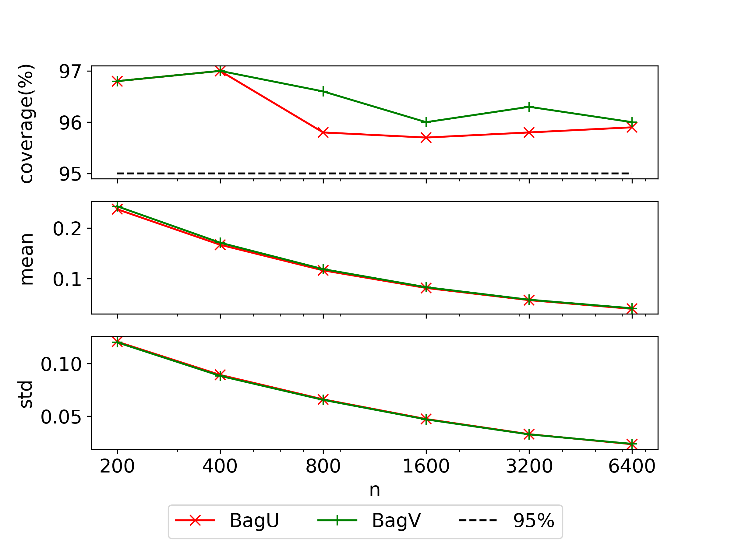
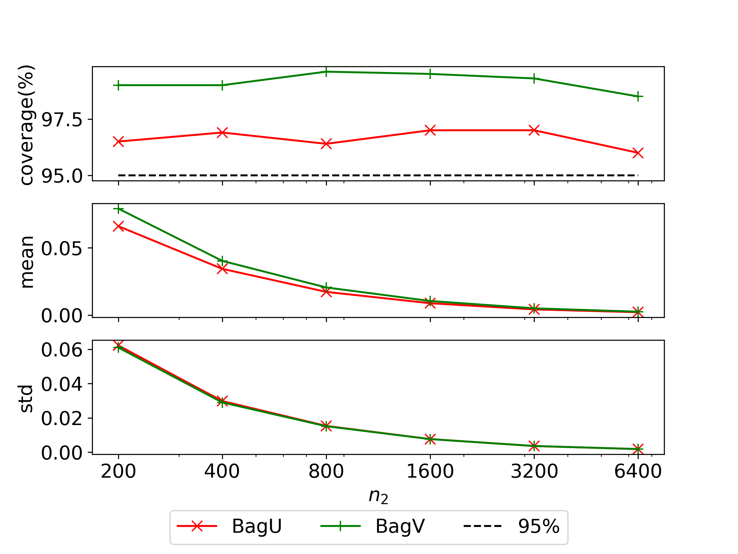
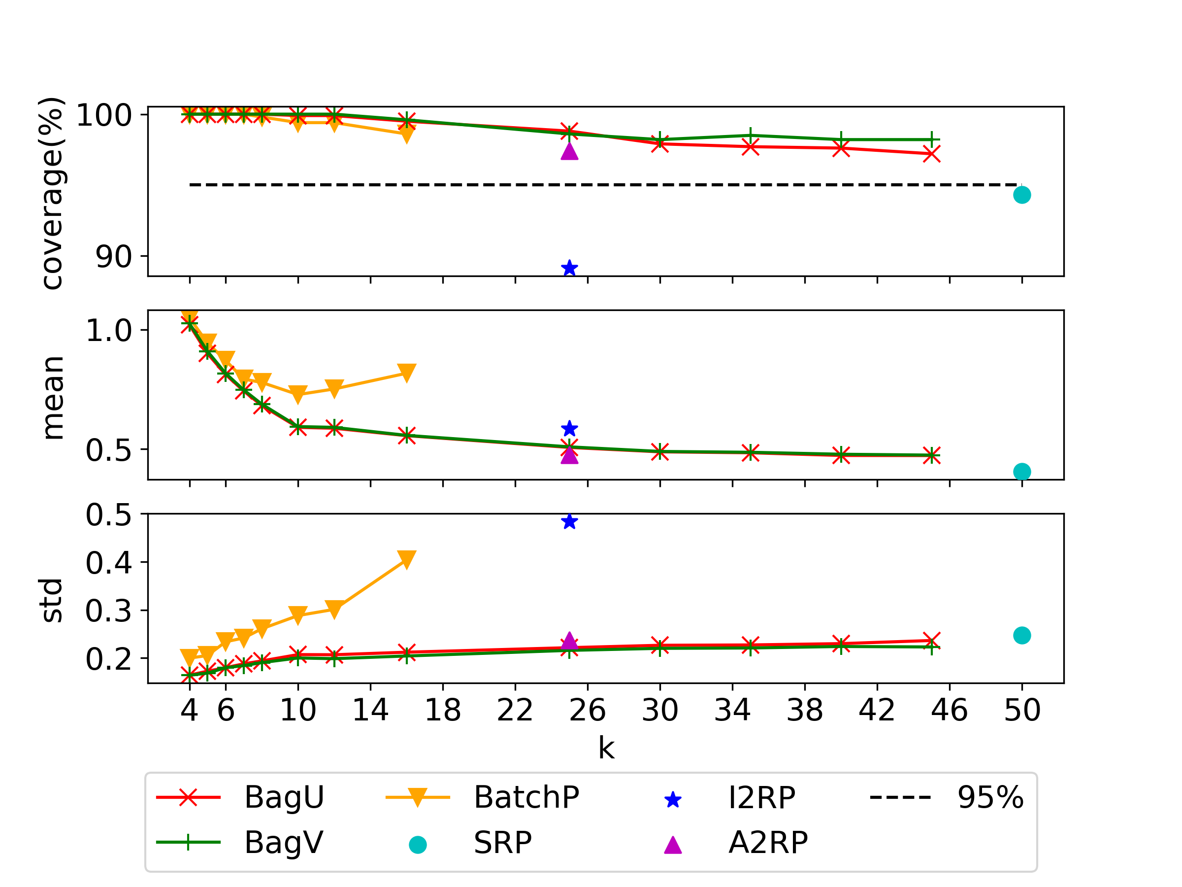
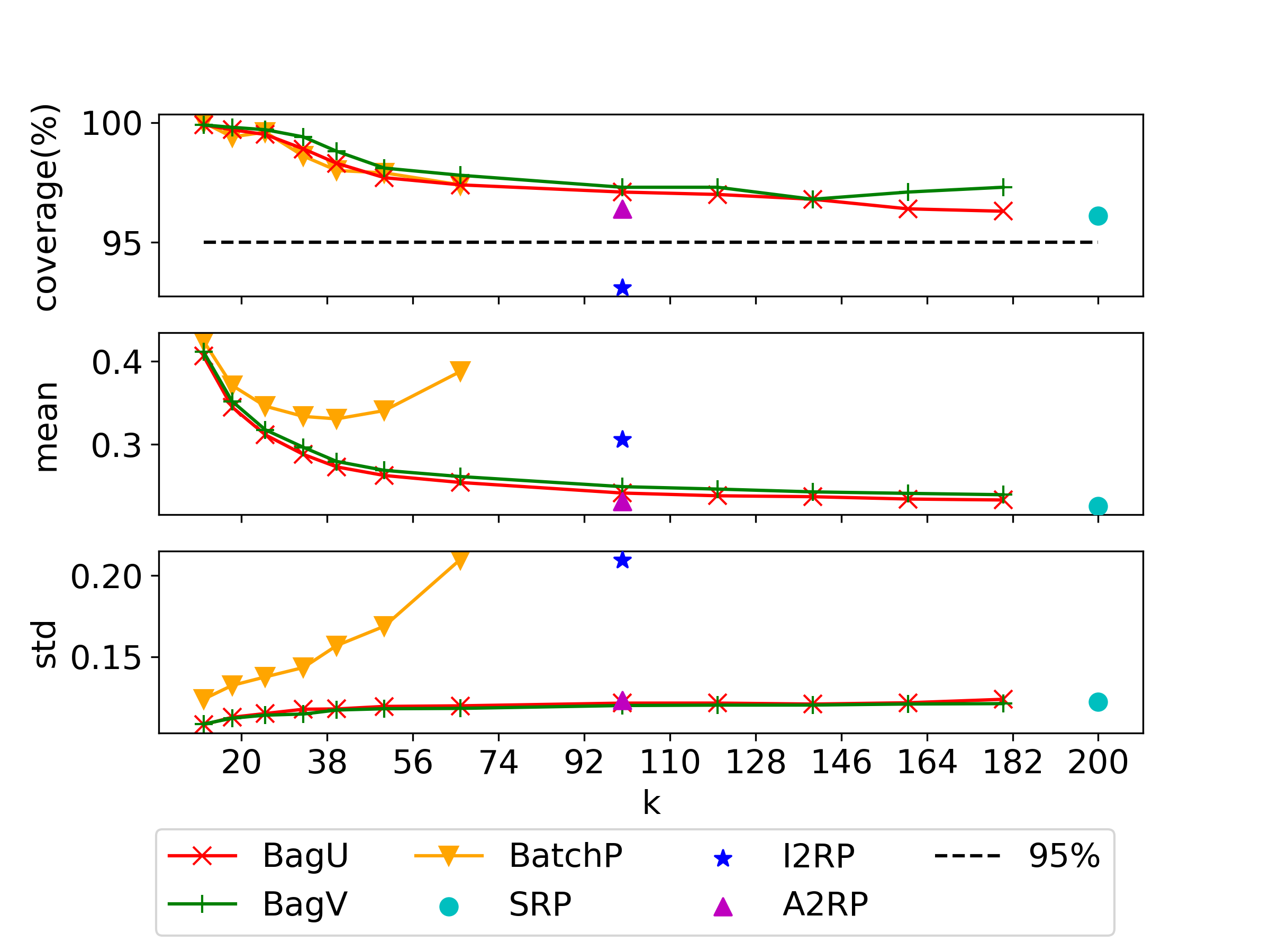
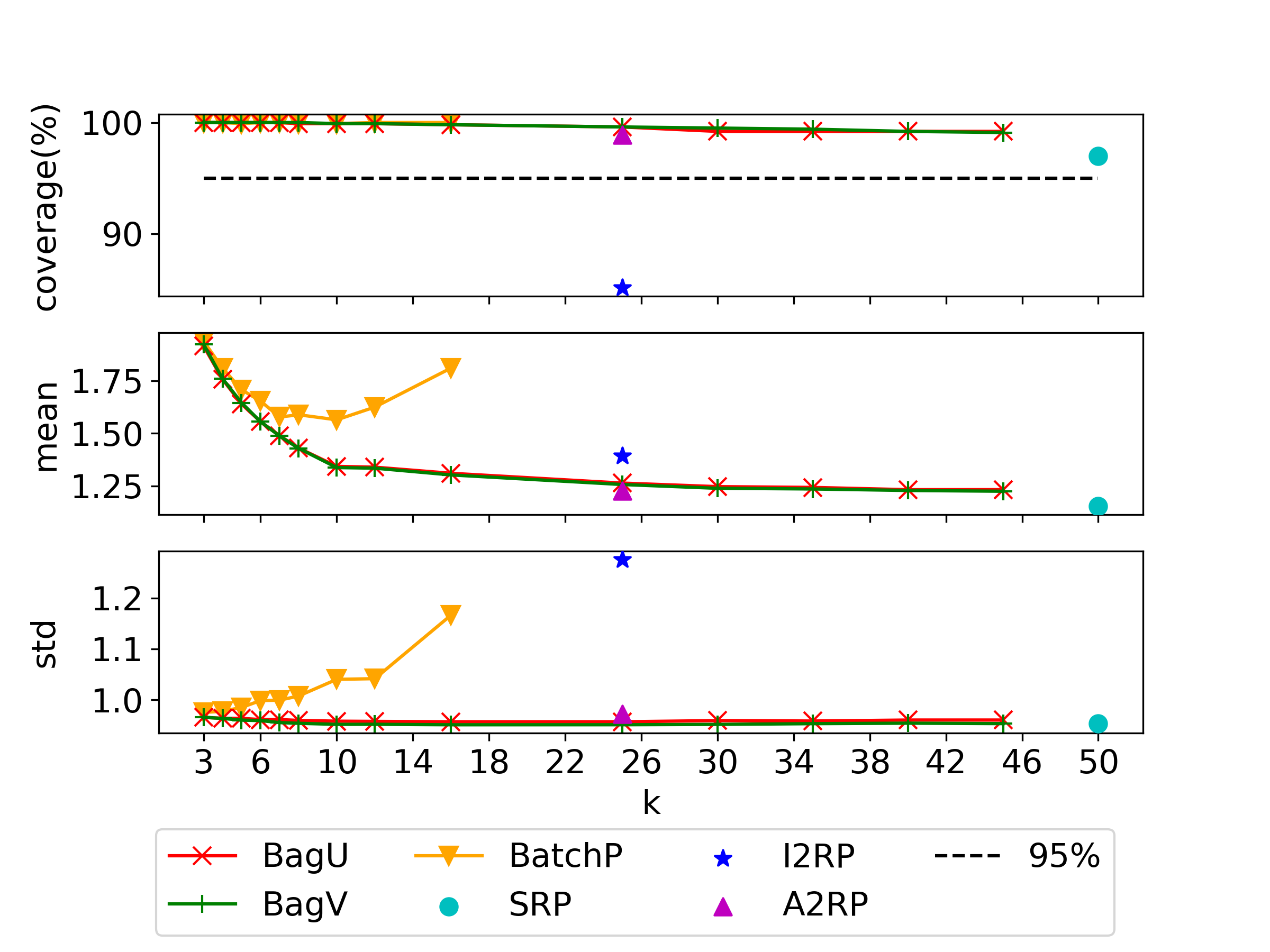
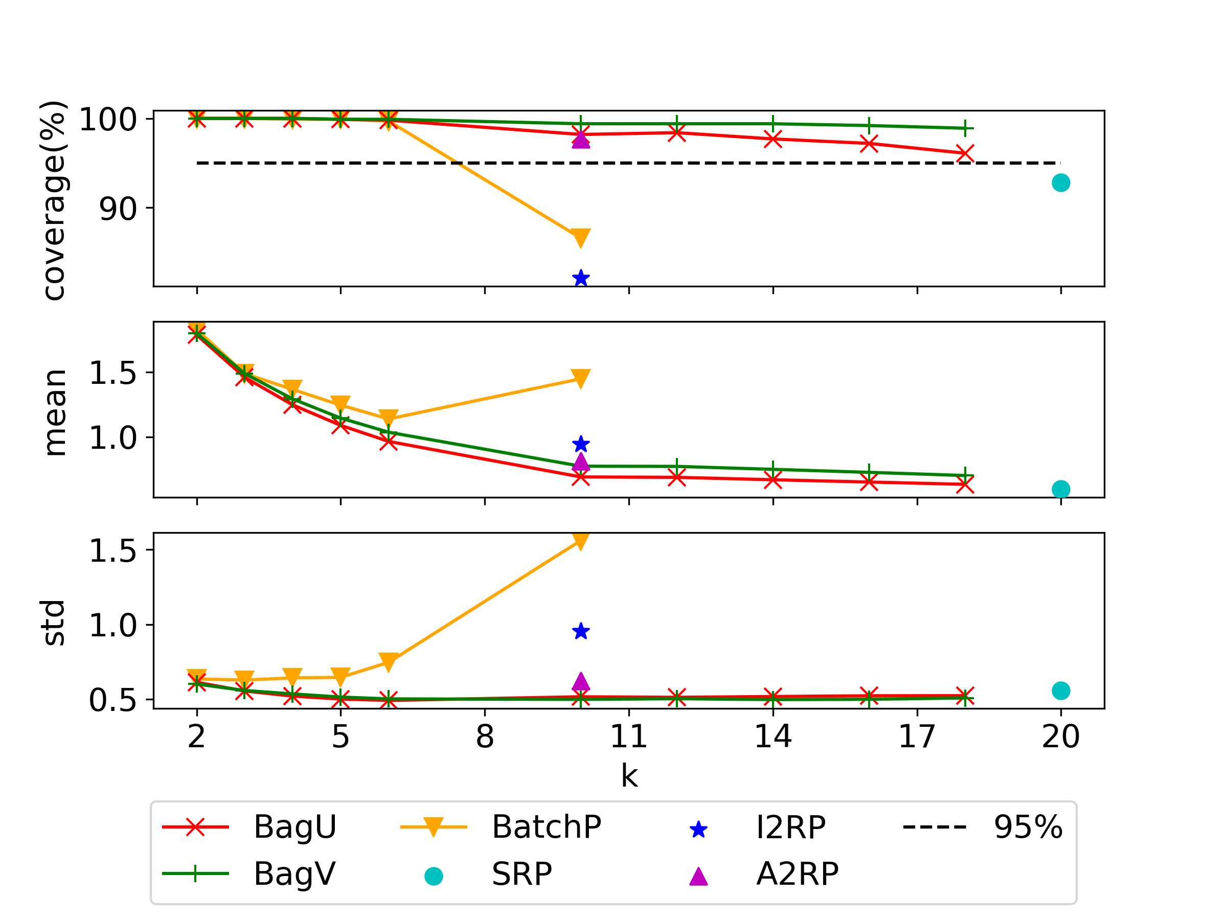
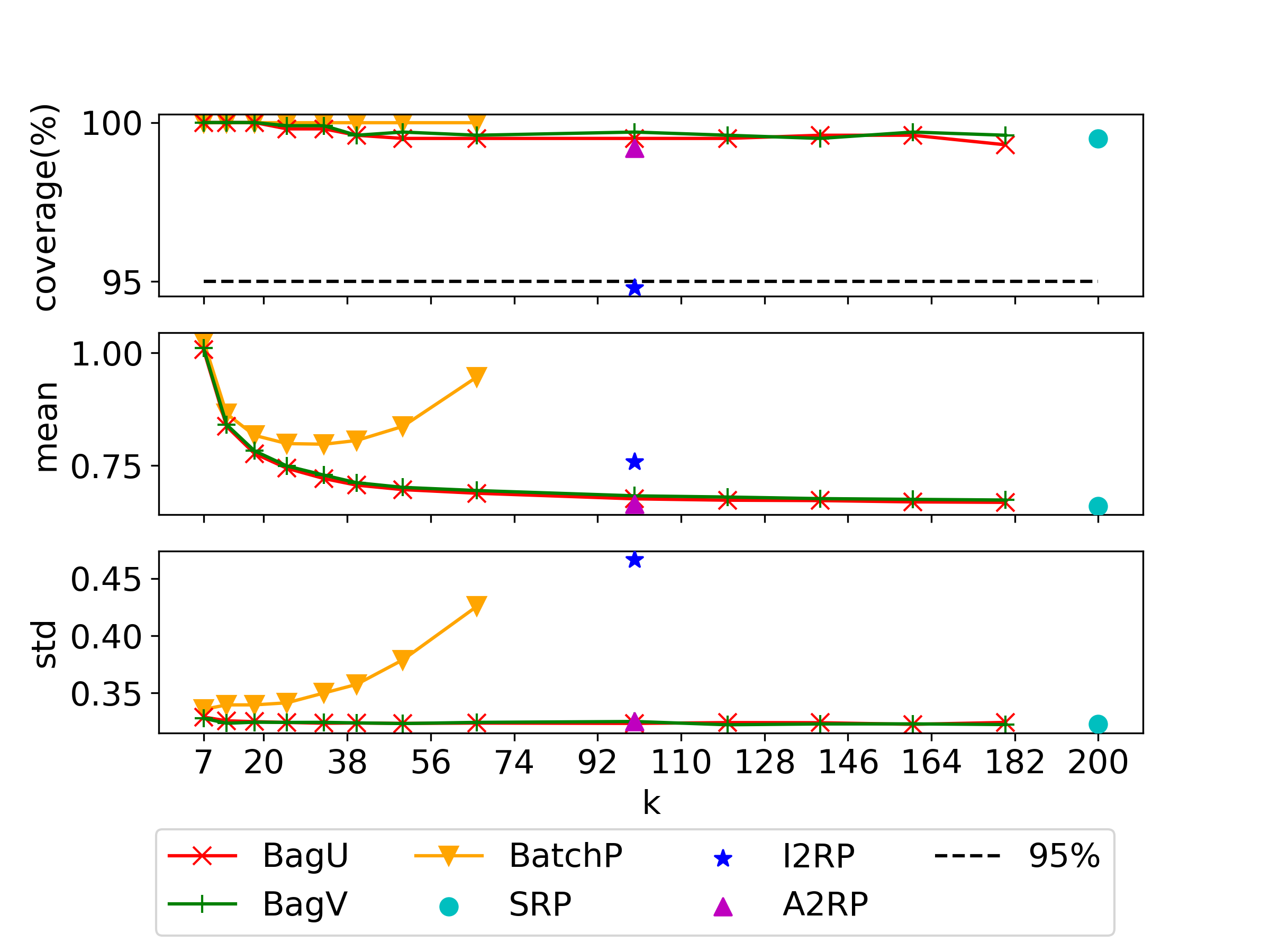
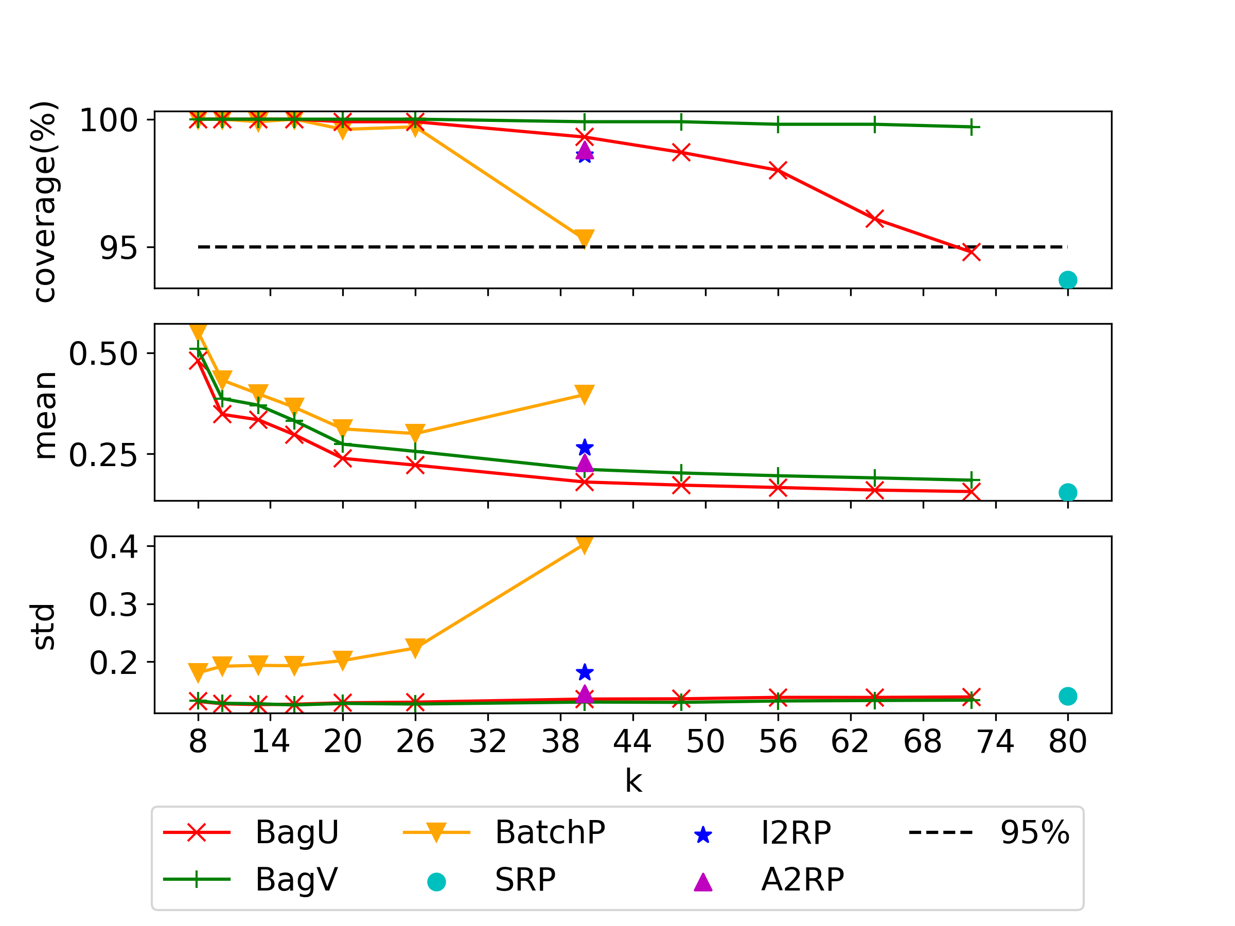
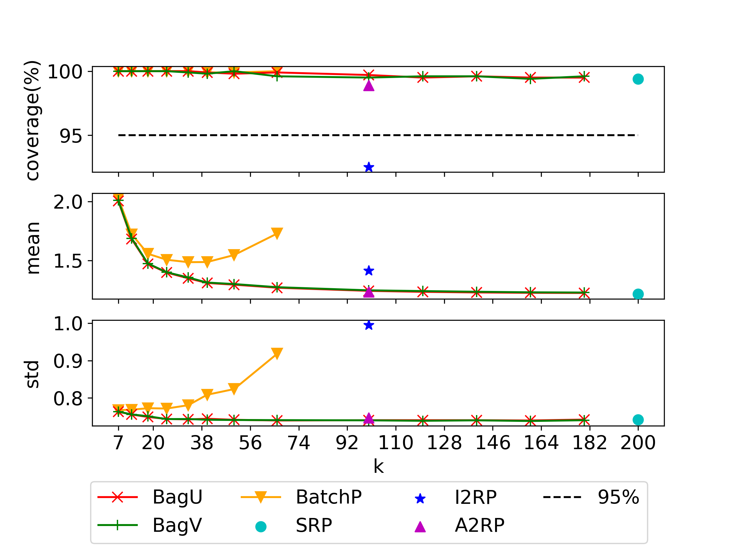
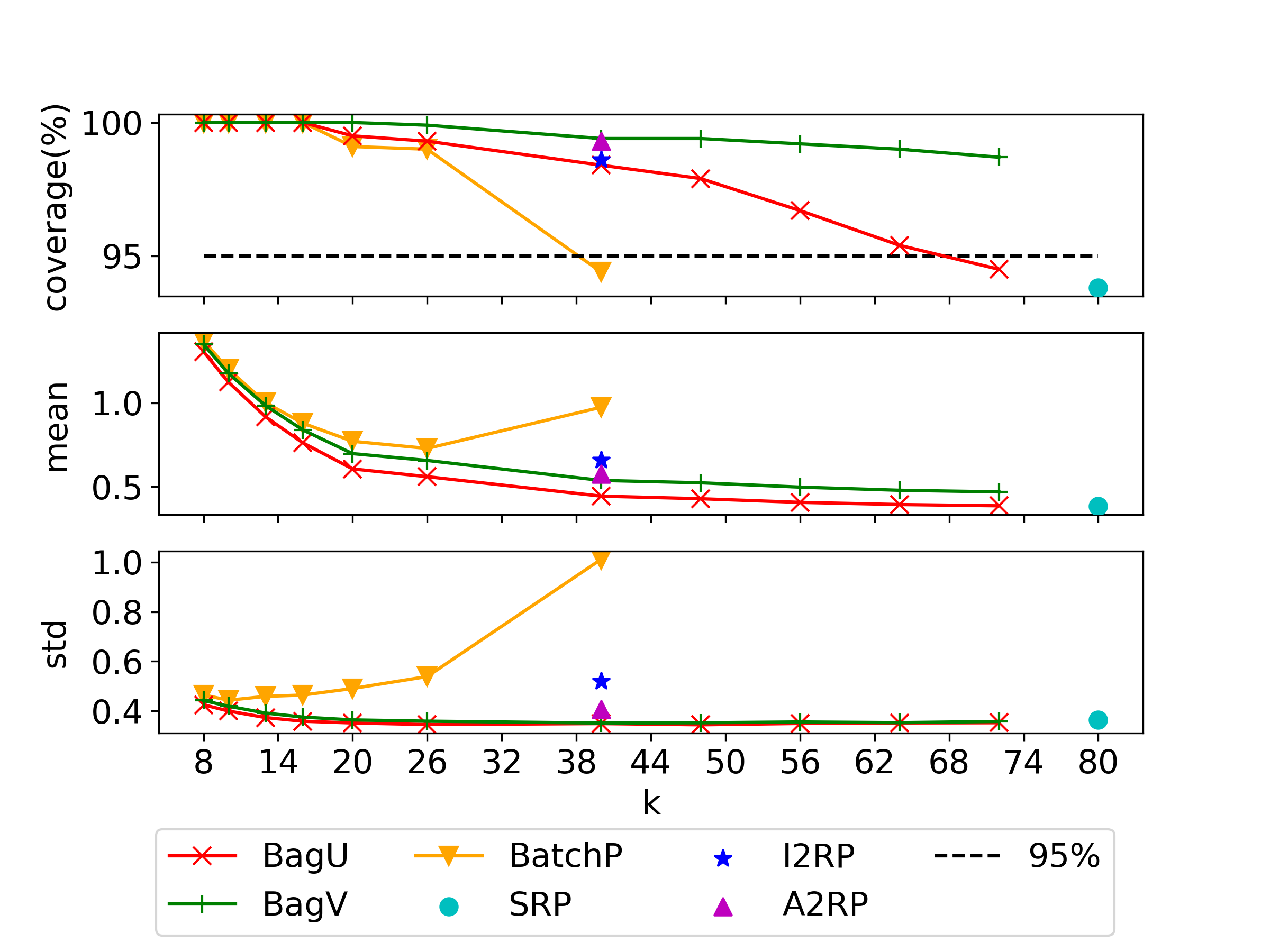
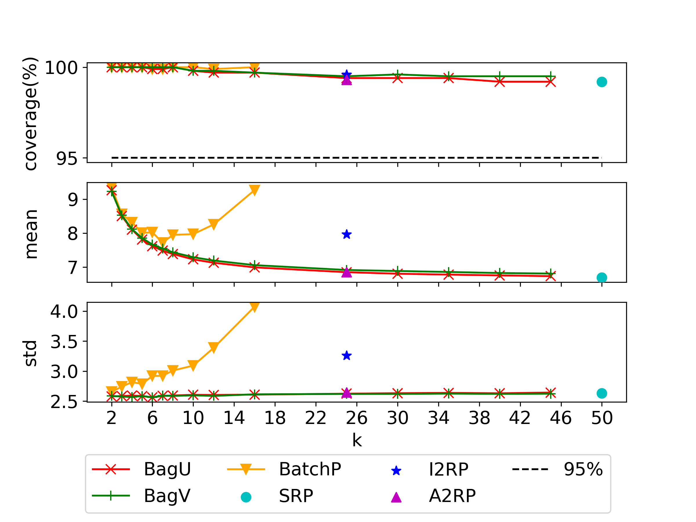
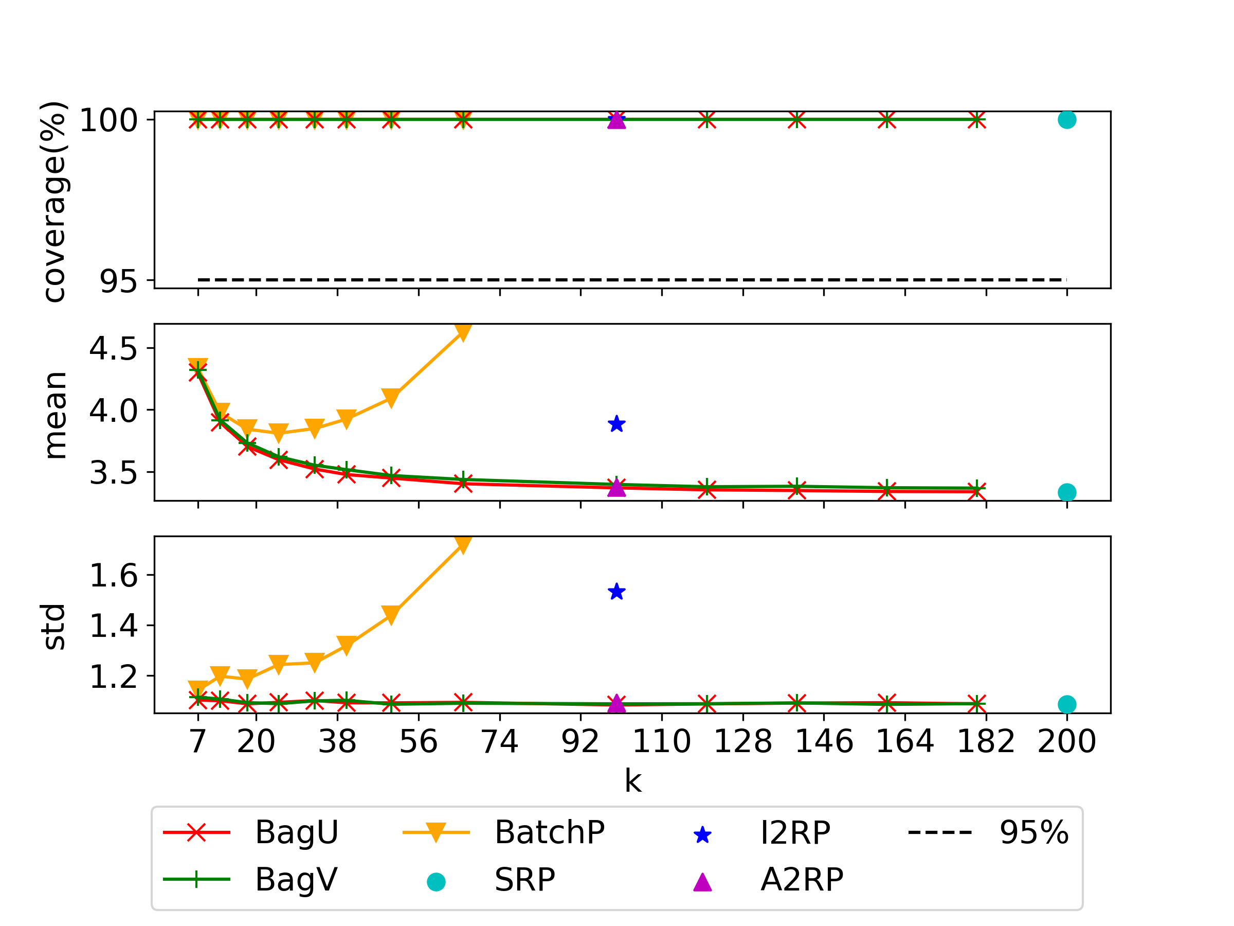
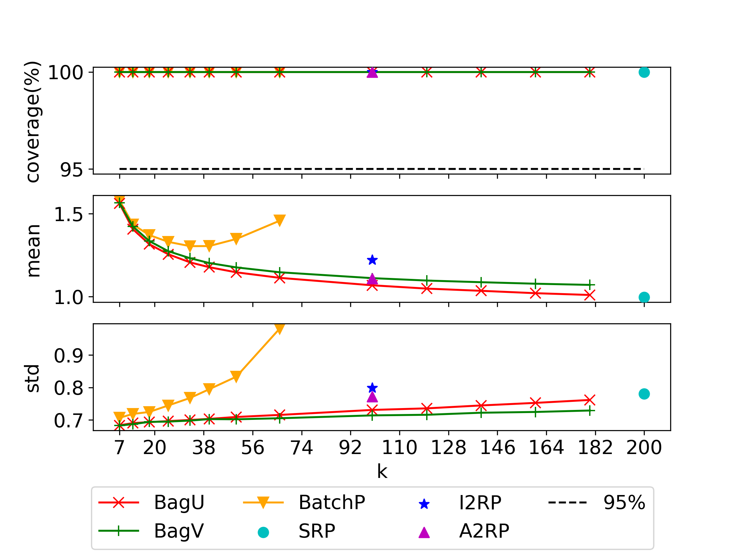
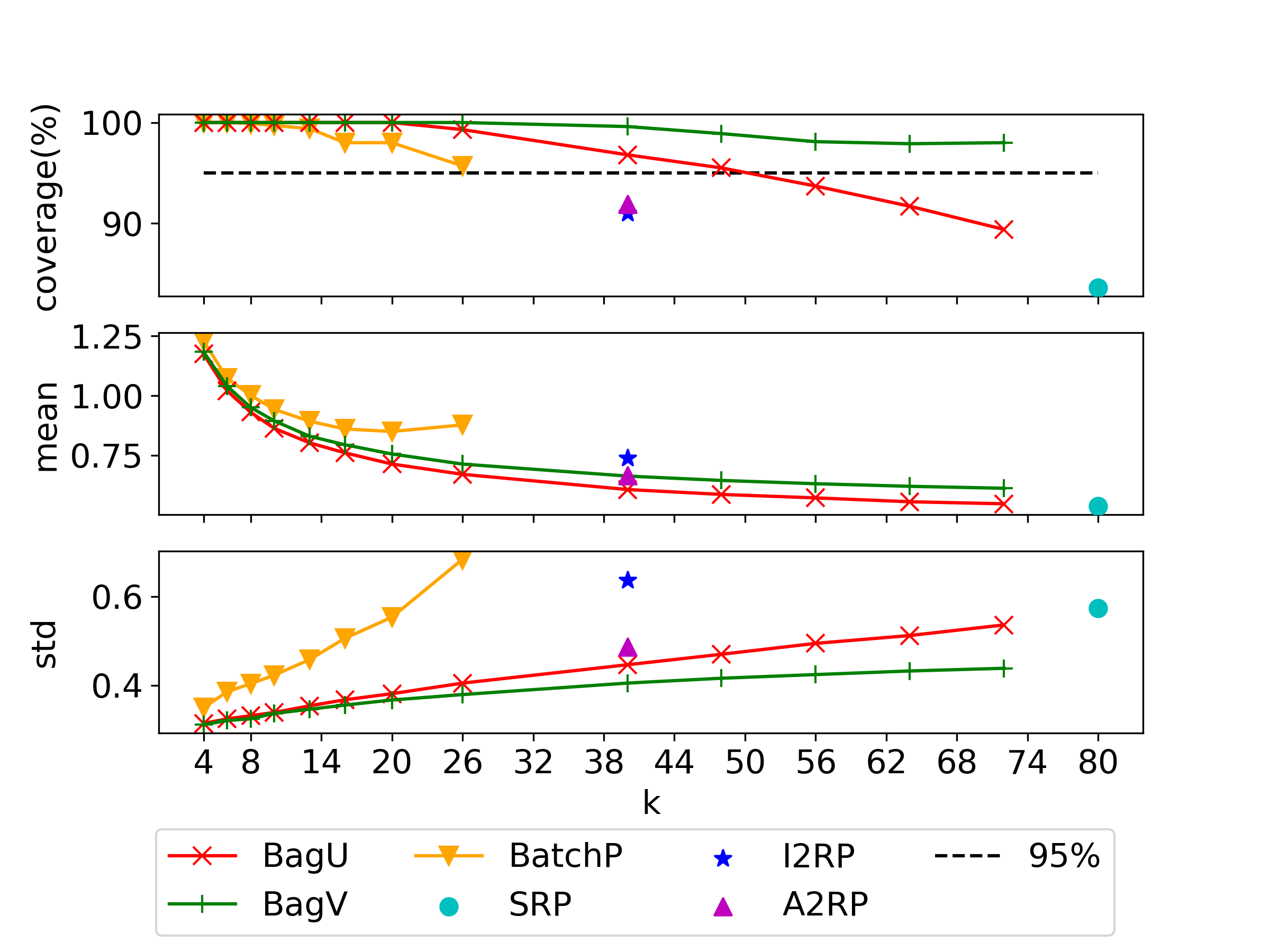
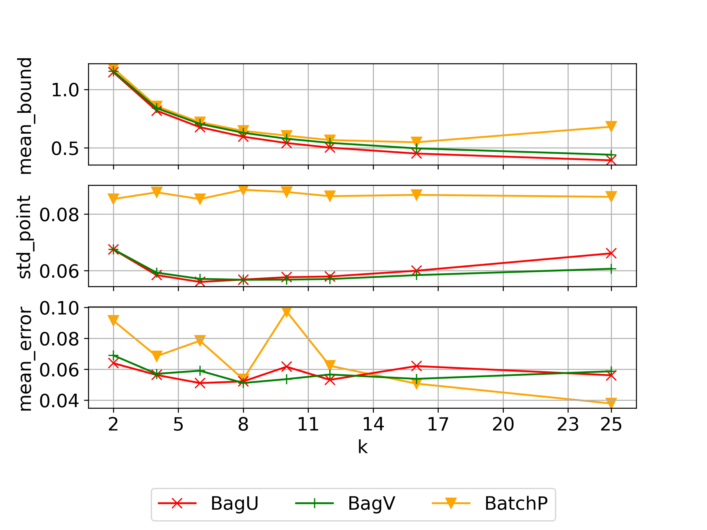
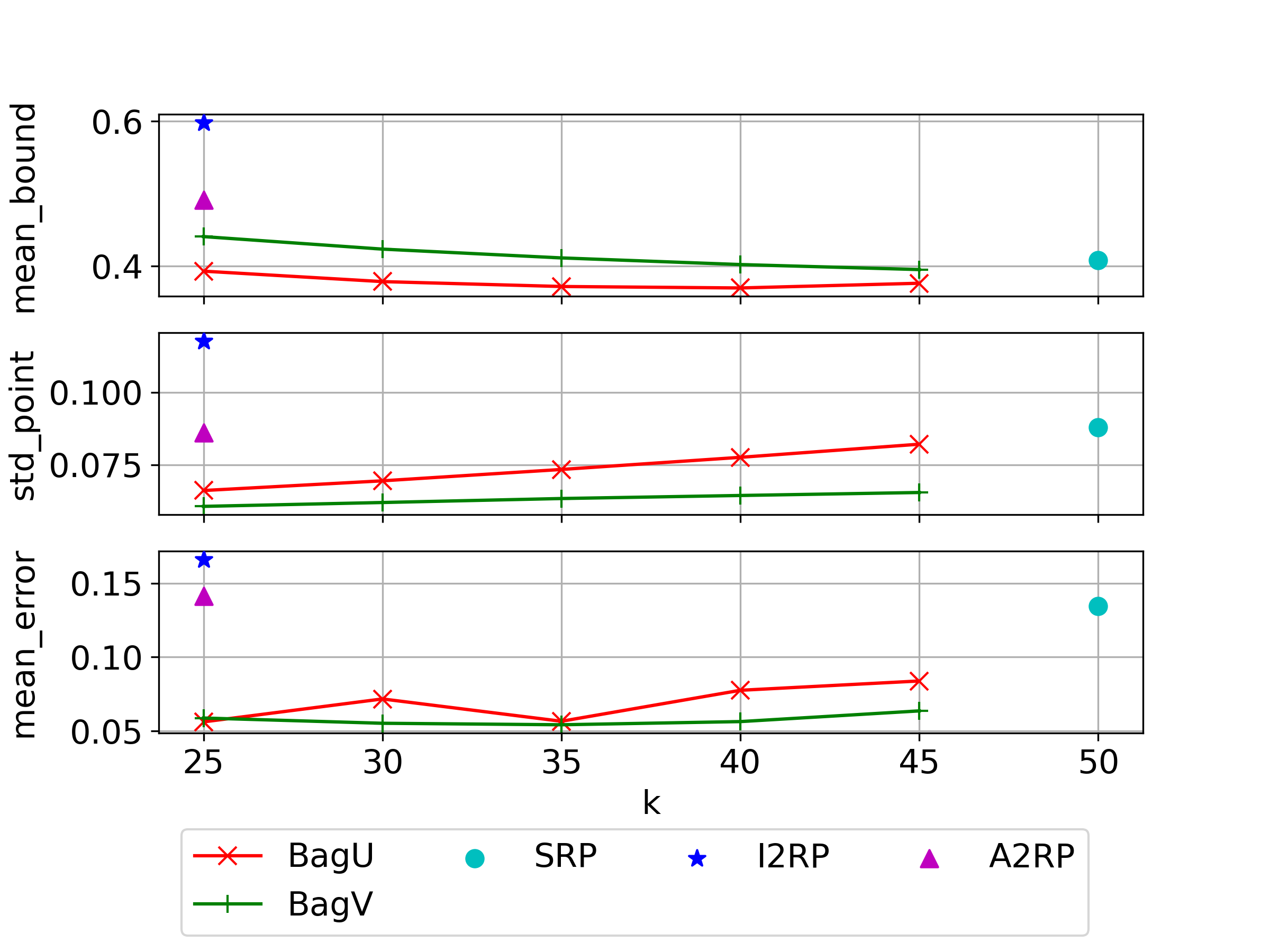
informs2014 \bibliographyAPXreferences
