CDF Transform-and-Shift: An effective way to deal with datasets of inhomogeneous cluster densities

Abstract

The problem of inhomogeneous cluster densities has been a long-standing issue for distance-based and density-based algorithms in clustering and anomaly detection. These algorithms implicitly assume that all clusters have approximately the same density. As a result, they often exhibit a bias towards dense clusters in the presence of sparse clusters. Many remedies have been suggested; yet, we show that they are partial solutions which do not address the issue satisfactorily. To match the implicit assumption, we propose to transform a given dataset such that the transformed clusters have approximately the same density while all regions of locally low density become globally low density—homogenising cluster density while preserving the cluster structure of the dataset. We show that this can be achieved by using a new multi-dimensional Cumulative Distribution Function in a transform-and-shift method. The method can be applied to every dataset, before the dataset is used in many existing algorithms to match their implicit assumption without algorithmic modification. We show that the proposed method performs better than existing remedies.

Keywords Density-ratio  $\cdot$ Density-based Clustering  $\cdot$ kNN anomaly detection  $\cdot$ inhomogeneous densities  $\cdot$ Scaling  $\cdot$ Shift

1 Introduction

Many existing distance-based and density-based algorithms in clustering and anomaly detection have an implicit assumption that all clusters have approximately the same density. As a result, these algorithms have a bias towards dense clusters and produce poor performance when presented with datasets having inhomogeneous cluster densities ². For example, DBSCAN ¹⁶ is biased towards grouping neighbouring dense clusters into a single cluster, in the presence of a sparse cluster ⁴⁴.

A number of methods have been proposed to “correct” this bias, but many of them are tailored to specific algorithms. For example, in the context of clustering, to overcome the issue of DBSCAN ¹⁶ that only uses a global density threshold to identify high-density clusters, OPTICS ⁵ utilises multiple density thresholds to extract clusters with varied densities based on a “reachability” (${k}^{th}$-nearest neighbour distance) plot. SNN clustering ¹⁵ proposes adaptive similarity measures in place of the distance measure in DBSCAN. In addition, DP ³⁴ identifies cluster centres which have local maximum density and are well separated, and then assigns each remaining point to its cluster centre via a linking scheme.

However, these methods are not satisfactory in addressing the density bias issue. The ranking on “reachability” plot of OPTICS depends heavily on the original data density distribution and the plot may merge different clusters which are close and dense ⁴⁴. The performance of SNN is sensitive to the $k$ setting in the ${k}^{th}$-nearest neighbour distance calculation that depends on the local data density ³⁸. Although DP uses local maximum density to identify cluster centres, the centre selection process is based on the density ranking on a decision graph ³⁴. In a nutshell, their performances are still affected by data density variation between clusters.

To demonstrate the shortcomings of these four density-based clustering algorithms, we apply them to an image segmentation task, and the data points are represented in the LAB space ³⁷. Table 1 shows their best clustering outcomes on the image shown in Figure 1. It can be seen that all these clustering algorithms cannot identify the sky, cloud and building well, due to the significant density variation in the LAB space.

Figure 1: An image used for segmentation.

Table 1: Image segmentation on the image shown in Figure 1. The colours in the scatter plot indicate different clusters identified by a clustering algorithm. The results only display the best-matched clusters wrt sky, cloud and buildings, i.e., the grey points in LAB scatter plots are labelled as noise or unmatched clusters by the clustering algorithm. We searched different parameters in a reasonable range. The bandwidth of the density estimator used in DBSCAN and DP is set to $\epsilon=0.1$.

	LAB	Cluster 1	Cluster 2	Cluster 3
DBSCAN
OPTICS
SNN
DP

Recently, density-ratio has been proposed as a principled method ⁴⁴ in addressing density bias. It aims to transform the data such that the estimated density of each transformed point approximates the density-ratio of that point in the original space. This effectively transforms locally low-density gaps between clusters in the original space into globally low-density gaps in the transformed space. As a result, all clusters can be easily extracted using a single density threshold.

On the same principle, we propose a more effective data transform-and-shift method based on a CDF (Cumulative Density Function). It transforms the space to one in which the cluster gaps are more obvious and all clusters have the same/similar density even though the geometry of each cluster may have changed. The proposed method is an elegant solution that equalises the density of all clusters (of high-density regions) as well as the density of low-density regions. This matches the implicit assumption of existing algorithms. The proposed method is a pre-processing method such that the transformed-and-shifted data can be used to reduce the underlying bias (towards dense clusters) and boost the performance of existing density-based algorithms without any algorithmic modification.

This paper makes the following three contributions:

1. Analysing the limitations and drawbacks of existing density-ratio based methods, i.e., existing CDF transform methods are either individual attribute-based (e.g., ReScale ⁴⁴) or individual point-based (e.g., DScale ⁴⁵); thus, they cannot solve the density bias issue adequately. More specifically, ReScale is a one-dimensional method which treats each dimension independently. The independent assumption limits its applications to some datasets only. DScale applies a multi-dimensional CDF without shifting; and it must be incorporated into an existing algorithm. DScale yields a non-metric and asymmetric measure. Both limit their ability to apply the transform multiple times in order to enhance the impact.

2. Proposing a new CDF-based Transform-and-Shift method called CDF-TS that changes the volume of each point’s neighbourhood simultaneously in the full multi-dimensional space. As far as we know, this is the first attempt to perform a multi-dimensional CDF transform to achieve the desired effect of homogenising the distribution of an entire dataset w.r.t a density estimator, i.e., making the density of all clusters homogeneous without impairing cluster structures.

3. Applying the new transform-and-shift method to both density-based clustering and distance-based anomaly detection to demonstrate its superiority over four existing algorithms, i.e., DBSCAN ¹⁶, DP ³⁴, LGD ²³, EC ⁴³; and one $k$NN anomaly detector.

The proposed method CDF-TS differs from the existing density-ratio algorithms of ReScale ⁴⁴ and DScale ⁴⁵ in three aspects:

1. Methodology: While ReScale ⁴⁴, DScale ⁴⁵ and the proposed CDF-TS follow the same principled method and have the same aim, the proposed CDF Transform-and-Shift method is a multi-dimensional technique incorporating both transformation and point-shift, which greatly expands the method’s applicability. In contrast, ReScale is a one-dimensional transformation and point-shift technique; and DScale is a multi-dimensional transformation without point-shift. The ‘complete’ CDF-TS method produces a more satisfactory result for both clustering and anomaly detection, which we will show in Section 7.

2. Metric compliance: CDF-TS and ReScale create a similarity matrix which is a metric; whereas the one produced by DScale ⁴⁵ is not a metric, i.e., it does not satisfy the symmetry or triangle inequalities. Thus, DScale cannot be used for algorithms that require the property of symmetry, e.g., we cannot visualise the scaled distance or data distribution using MDS ⁸.

3. Ease of use: Like ReScale, CDF-TS is a preprocessing method to transform data. The targeted (clustering or anomaly detection) algorithm can thus be applied without altering to the transformed data. In contrast, DScale requires an algorithmic modification before using it.

The rest of the paper is organised as follows. The related work in a broader context is described in Section 2. The most closely related work is organised into the following three sections. Section 3 presents the issues of inhomogeneous cluster density in density-based clustering and distance-based anomaly detection. Section 4 describes the density-ratio estimation as a principle to address the issues of inhomogeneous density. Section 5 presents the two existing CDF scaling methods based on density-ratio. Section 6 proposes the local-density transform-and-shift as a multi-dimensional CDF scaling method. Section 7 empirically evaluates the performance of existing density-based clustering and distance-based anomaly detection algorithms on the transformed-and-shifted datasets. Discussion and conclusions are provided in the last two sections.

2 Related work in a broader context

There are many algorithms proposed to improve density-based clustering performance on a dataset with clusters of varied densities. OPTICS ⁵ and HDBSCAN ¹⁰ utilise different thresholds to extract clusters of different densities. IS-DBSCAN ¹¹, DP ³⁴, LC ¹², LGD ²³, DPC-DBFN ²⁶ and EC ⁴³ rely on local density estimation. IS-DBSCAN ¹¹ uses a ranking procedure based on the kNN distances to efficiently identify different densities in the dataset. DP ³⁴ identifies cluster modes which have local maximum density and are well separated, and then assigns each remaining point in the dataset to a cluster mode via a linking scheme. LC ¹² and DPC-DBFN ²⁶ utilise enhanced local density estimators based on a kNN graph and a fuzzy neighbourhood measure, respectively, to improve the clustering performance of DP. EC ⁴³ redefines cluster centres as points with the highest density in their neighbourhoods to overcome the shortages of DP. To handle high-dimensional data with varied densities, LGD ²³ estimates the local density for each point based on the average distance over the nearest neighbours of that point. In addition, MuDi-Stream ⁴ uses a grid-based method to detect adaptive micro-clusters for clustering streaming data with clusters of varied densities. MDSC ¹⁷ uses a swarm intelligence approach to adaptively merge micro-clusters and improve the performance of clustering dynamic data streams.

ReScale ⁴⁴ and DScale ⁴⁵ are density-ratio based scaling methods which are able to improve existing density-based clustering algorithm on detecting clusters with varied densities. In addition, there are data-dependent similarity measures, such as SNN ¹⁵ and aNNE ³¹, which can be directly applied on an existing density-based clustering algorithm to overcome their weakness of detecting varied densities.

LOF ⁹ is a local density-based approach for anomaly detection. The LOF score of $x$ is the ratio of the average density of $x$’s $k$-nearest neighbours to the density of $x$, where the density of $x$ is inversely proportional to the average distance to its $k$-nearest-neighbours ⁹. It has the ability to identify local anomalies, which are relatively low-density points close to a dense cluster. With an isolation-based approach to detect local anomalies, iNNE ⁶ uses a nearest neighbour ensemble to calculate a ratio of nearest neighbour distances.

There are many unsupervised distance metric learning algorithms which aim to transform data from a high-dimensional space to a low-dimensional space, e.g., global methods such as PCA ²¹ and KUMMP ⁴²); and local methods such as Isomap ³⁹ and t-SNE ²⁷. These methods are usually used as dimension reduction methods such that data clusters are transformed into a low-dimensional space based on some local/global objective function in linear/nonlinear approaches ^{7, 41}. For example, t-SNE ²⁷ first uses the Gaussian kernel to convert similarities between data points to joint probabilities in the original space. Then it produces a low-dimensional space that minimises the Kullback-Leibler divergence between the joint probabilities of the low-dimensional space and the original space.

The objective of CDF-TS is to reduce the density variation of a given dataset that yields a transformed dataset with clusters of homogeneous density. And this is achieved without impairing the cluster structures and changing the dimensionality in the given dataset. The transform step employs CDF; the shift step shifts data points based on the local density distribution in the original space. None of the distance metric learning algorithms has this objective, or employs the CDF transform and/or point shift as a methodology. The objective of CDF-TS is specifically targeted to reduce the underlying bias (towards dense clusters) in density-based algorithms. In contrast, metric learning algorithms are generic dimensional reduction methods, often targeted for visualisation. With reference to the categorisation of local/global and linear/nonlinear methods in distance metric learning, CDF-TS uses a linear method to do the CDF transform; and it is a local method because of the use of local density distribution.

In a nutshell, CDF-TS is neither a metric learning method nor a dimension reduction method.

As mentioned in the last section, algorithms using a method closely related to that of CDF-TS are ReScale ⁴⁴ and DScale ⁴⁵. With the differences mentioned earlier, we will show that CDF-TS greatly expands the method’s applicability and enables different density estimators to be employed in both clustering and anomaly detection tasks.

3 Effect of inhomogeneous cluster densities

We now discuss the effect of inhomogeneous cluster densities on density-based clustering and distance-based anomaly detection algorithms.

3.1 Density-based clustering

This section describes the condition under which density-based algorithm DBSCAN fails to detect all clusters in a dataset of inhomogeneous cluster densities.

Let $D=\{x_{1},x_{2},...,x_{n}\}$, $x_{i}\in\mathbb{R}^{d},x_{i}\sim F$ denote a dataset of $n$ points, each sampled independently from a distribution $F$. Let $\widehat{pdf}(x)$ denote the density estimate of point $x$ which approximates the true density $pdf(x)$. In addition, let $\mathcal{N}(x;\epsilon)$ be the $\epsilon$-neighbourhood of $x$, $\mathcal{N}(x;\epsilon)=\{y\in D\leavevmode\nobreak\ |\leavevmode\nobreak\ s(x,y)\leqslant\epsilon\}$, where $s(\cdot,\cdot)$ is the distance function ($s:{\mathbb{R}}^{d}\times{\mathbb{R}}^{d}\rightarrow{\mathbb{R}}$).

The classic density-based clustering algorithm DBSCAN ¹⁶, estimates the density ${pdf}(x)$ of a point $x$ by counting points within a small $\epsilon$-neighbourhood as follows:

$$\widehat{pdf}_{\epsilon}(x)=\frac{1}{nV_{\epsilon}}|\mathcal{N}(x;\epsilon)|=\frac{|\{y\in D\leavevmode\nobreak\ |\leavevmode\nobreak\ s(x,y)\leqslant\epsilon\}|}{nV_{\epsilon}}$$ (1)

where $V_{\epsilon}\propto\epsilon^{d}$ is the volume of a $d$-dimensional ball of radius $\epsilon$.

A set of clusters $\{C_{1},\dots,C_{\varsigma}\}$ is defined as non-empty and non-intersecting subsets: $C_{i}\subset D,C_{i}\neq\emptyset,\forall_{i\neq j}\ C_{i}\cap C_{j}=\emptyset$. Let $c_{i}=\arg\max_{{x\in C_{i}}}\widehat{pdf}(x)$ denote the mode (point of the highest estimated density) for cluster $C_{i}$; $p_{i}=\widehat{pdf}(c_{i})$ denote the corresponding peak density value.

DBSCAN uses a global density threshold to identify core points (which have densities higher than the threshold); then it links neighbouring core points together to form clusters ¹⁶. It is defined as follows.

Definition 1.

A core point is a point with an estimated density above or equal to a user-specified threshold $\tau$, i.e., $(\widehat{pdf}_{\epsilon}(x)\geqslant\tau)\leftrightarrow Core(x)=1$, where $Core$ denotes a set indicator function.

Definition 2.

Using a density estimator with density threshold $\tau$, a point $x_{1}$ is density connected with another point $x_{p}$ in a sequence of $p$ unique points from $D$, i.e., $\{x_{1},x_{2},x_{3},...,x_{p}\}$: $CON_{\epsilon}^{\tau}(x_{1},x_{p})$ is defined as:

$$CON_{\epsilon}^{\tau}(x_{1},x_{p})\leftrightarrow\left\{\begin{array}[]{l}\text{(i) if $p=2$}:(x_{1}\in\mathcal{N}_{\epsilon}(x_{p}))\wedge(Core(x_{1})\vee Core(x_{p}));\\ \text{(ii) if $p>2$}:\exists_{(x_{1},x_{2},...x_{p})}((\forall_{i\in\{2,...,p\}}\ x_{i-1}\in\mathcal{N}_{\epsilon}(x_{i}))\wedge(\forall_{i\in\{2,...,p-1\}}\ Core(x_{i}))).\end{array}\right.$$

Definition 3.

A cluster detected by the density-based algorithm DBSCAN is a maximal set of density connected instances, i.e., ${C}_{i}=\{x\in D\ |\ CON_{\epsilon}^{\tau}(x,c_{i})\}$, where $c_{i}=\arg\max_{\begin{subarray}{c}x\in\mathbb{C}_{i}\end{subarray}}\widehat{pdf}_{\epsilon}(x)$ is the cluster mode.

For this kind of algorithm to find all clusters in a dataset, the data distribution must have the following necessary condition: the peak density of each cluster must be greater than the maximum over all possible paths of the minimum density along any path linking any two modes. This condition is formally described by Zhu et al ⁴⁴ as follows:

$$\min_{{k\in\{1,\dots,\varsigma\}}}c_{k}>\max_{{i\neq j\in\{1,\dots,\varsigma\}}}g_{ij}$$ (2)

where $g_{ij}$ is the largest of the minimum density along any path linking the mode of clusters $C_{i}$ and $C_{j}$.

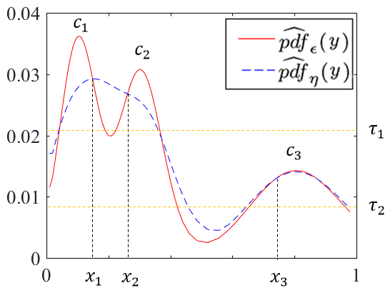
This condition implies that there must exist a threshold $\tau$ that can be used to break all paths between the modes by assigning regions with a density less than $\tau$ to noise. Otherwise, if some cluster mode has a density lower than that of a low-density region between other clusters, then this kind of density-based clustering algorithm will fail to find all clusters. Either some high-density clusters will be merged (when a lower density threshold is used), or low-density clusters will be designated as noise (when a higher density threshold is used). To illustrate, Figure 2(a) shows that using a high threshold $\tau_{1}$ will cause all points in Cluster $C_{3}$ to be assigned to noise but using a low threshold $\tau_{2}$ will cause points in $C_{1}$ and $C_{2}$ to be assigned to the same cluster.

(a) Original data

(b) ReScaled data

Figure 2: (a) A mixture of three one-dimensional Gaussian distributions that cannot be separated using a single density threshold; (b) Density distribution on ReScaled data of (a), where a single density threshold can be found to separate all three clusters. Note that point $x_{1}$, $x_{2}$ and $x_{3}$ are shifted to $y_{1}$, $y_{2}$ and $y_{3}$, respectively. $\eta$ is a larger bandwidth than $\epsilon$.

3.2 $k$NN anomaly detection

A classic nearest-neighbour based anomaly detection algorithm assigns an anomaly score to an instance based on its distance to the $k$-th nearest neighbour ³². The instances with the largest anomaly scores are identified as anomalies.

On a dataset of inhomogeneous cluster densities, we show that this kind of anomaly detector fails to detect two types of anomalies, i.e., local anomalies and anomalous clusters.

Given a dataset and the parameter $k$, the density of $x$ can be estimated using a $k$-th nearest neighbour density estimator (as used by the classic $k$NN anomaly detector ³²):

$$\widehat{pdf}_{\epsilon_{k}(x)}(x)=\frac{1}{nV_{\epsilon_{k}(x)}}|\mathcal{N}(x;\epsilon_{k}(x))|=\frac{k}{n\times V_{\epsilon_{k}(x)}}\propto(\frac{1}{\epsilon_{k}(x)})^{d}$$ (3)

where $\epsilon_{k}(x)$ is the distance between $x\in\mathbb{R}^{d}$ and its $k$-th nearest neighbour in a dataset $D$.

Note that the $k$-th nearest neighbour distance $\epsilon_{k}(x)$ is a proxy to the density of $x$, i.e., high $\epsilon_{k}(x)$ indicates low density, and vice versa.

Let $C$ be the set of all normal points in a dataset $D$. The condition under which the classic $k$NN anomaly detector could, with an appropriate setting of a density/distance threshold, identify every anomaly $y$ in $A=D\setminus C$ is given as follows:

$$\min_{y\in A}\ \epsilon_{k}(y)>\max_{x\in C}\ \epsilon_{k}(x)$$ (4)

Equation 4 states that all anomalies must have the highest $k$NN distances (or the lowest densities) in order to detect them. In other words, $k$NN anomaly detectors can detect both global anomalies and scattered anomalies which have lower densities than that of all normal points ^{1, 25}.

However, based on this characteristic, $k$NN anomaly detectors are unable to detect:

1. Local anomalies. This is because a local anomaly $y$ with low density relative to nearby normal (non-anomalous) instances in a region of high average density may still have a higher density than that of normal (non-anomalous) instances in regions of lower average density ⁹. Translating this in terms of $k$-th NN distance, we have: $\forall_{x,z\in C,y\in A}\ \epsilon_{k}(x)<\epsilon_{k}(y)<\epsilon_{k}(z)$. Here, some local anomalies (for example, points located around the boundaries of $C_{1}$ and $C_{2}$) are ranked lower than the normal points located around the sparse cluster ($C_{3}$), as shown in Figure 2(a).

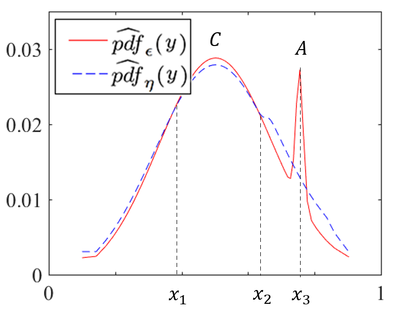
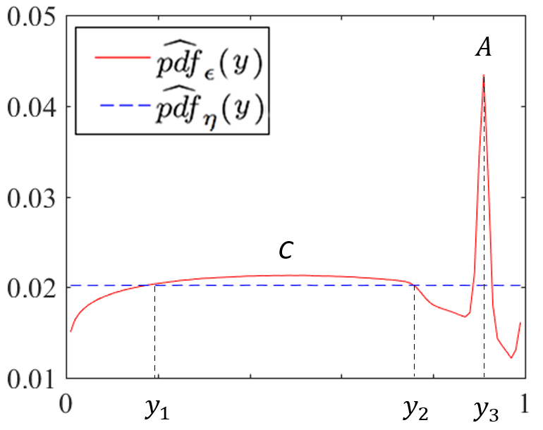
2. Anomalous clusters (sometimes referred to as clustered anomalies ²⁵) are groups of points where each group is too small to be considered a normal cluster and is found in a low-density region of the space (i.e. far from the other normal clusters). They are difficult to detect when the density of each point of an anomalous cluster is higher than most normal points. A purported benefit of the $k$NN anomaly detector is that it is able to identify such anomalous clusters provided $k$ is sufficiently large (larger than the size of the anomalous group), when these clustered anomalies are sufficiently distanced from normal points ¹. By rescaling the data such that clustered anomalies could be farther to the normal points, larger $k$NN distances could be used to detect them.

(a) Original data

(b) ReScaled data

Figure 3: (a) A mixture of two one-dimensional Gaussian distributions where C is a normal cluster and A is an anomalous cluster; (b) Density distribution on the ReScaled data of (a), where the anomalous cluster is farther to the normal cluster centre. Note that point $x_{1}$, $x_{2}$ and $x_{3}$ are shifted to $y_{1}$, $y_{2}$ and $y_{3}$, respectively.

To sum up, both density-based clustering and distance-based anomaly detectors have weaknesses when it comes to handling datasets with inhomogeneous cluster densities clusters. Rather than creating a new density estimator or modifying the existing clustering and anomaly detection algorithm procedures, we advocate transforming clusters to be more uniformly distributed (with homogeneous density) than it is in the original space such that the separation between clusters can be identified easily.

4 Density-ratio estimation

Density-ratio estimation is a principled method to overcome the weakness of density-based clustering for detecting clusters with inhomogeneous densities ⁴⁴.

The density-ratio of a point is the ratio of two density estimates calculated using the same density estimator, but with two different bandwidth settings.

Let $pdf(\cdot;\gamma)$ and $pdf(\cdot;\lambda)$ be density estimators using kernels of bandwidth $\gamma$ and $\lambda$, respectively. Given the constraint that the denominator has a larger bandwidth than the numerator $\gamma<\lambda$, the density ratio of $x$ is estimated as:

$${rpdf}(x;\gamma,\lambda)=\frac{{pdf}(x;\gamma)}{{pdf}(x;\lambda)}$$ (5)

We recall a lemma from ⁴⁴ regarding the density ratio:

Lemma 1.

For any data distribution and sufficiently small values of $\gamma$ and $\lambda$ s.t. $\gamma<\lambda$, if $x$ is at a local maximum density of $\mathcal{N}(x;\lambda)$, then ${rpdf}(x;\gamma,\lambda)\geqslant 1$; and if $x$ is at a local minimum density of $\mathcal{N}(x;\lambda)$, then ${rpdf}(x;\gamma,\lambda)\leqslant 1$.

Since points located at local high-density areas (almost invariably) have density-ratio higher than points located at local low-density areas, a global density-ratio threshold around unity can be used to identify all cluster peaks and break all paths between different clusters. Thus, based on density-ratio estimation, existing density-based clustering algorithms such as DBSCAN can identify clusters as regions of locally high density, separated by regions of locally low density.

Similarly, a density-based anomaly detector is able to detect local anomalies since their density-ratio values are lower and ranked higher than normal points with locally high densities.

5 Scaling inhomogeneous cluster densities

We now discuss methods for rescaling a dataset to tackle the problem of inhomogeneous cluster densities.

5.1 One-dimensional CDF scaling

Let $pdf(\cdot;\lambda)$ and $cdf(\cdot;\lambda)$ denote density and cumulative-density estimators, respectively, which are parameterised by a bandwidth of $\lambda$. Let $x^{\prime}$ denote a point that has been transformed using the $cdf$ as follows:

$$x^{\prime}=cdf(x;\lambda)$$ (6)

As this is a probability integral transform ³⁰, we then have the property:

$$pdf(x^{\prime};\lambda)=pdf(cdf(x;\lambda);\lambda)=1/n$$ (7)

Given the data size $n$ is large, $pdf(x)$ varies slowly around $x$ and $\lambda>\gamma$, we have ⁴⁴:

$$pdf(x^{\prime};\gamma) = \frac{1}{nV_{\gamma}}\sum_{j}\mathbf{1}(\|{x^{\prime}-x^{\prime}_{j}}\|\leqslant\gamma)$$ (8)

$$= \frac{1}{nV_{\gamma}}\sum_{j}\mathbf{1}(\|{cdf(x;\lambda)-cdf(x_{j};\lambda)}\|\leqslant\gamma)$$

$$\approx \frac{1}{nV_{\gamma}}\sum_{j}\mathbf{1}(pdf(x;\lambda)*\|{x-x_{j}}\|\leqslant\gamma)$$

$$\approx \frac{1}{V_{\gamma}}P_{X\sim F}(pdf(x;\lambda)*\|{x-X}\|\leqslant\gamma)$$

$$= \frac{1}{V_{\gamma}}P_{X\sim F}(\|{x-X}\|\leqslant\frac{\gamma}{pdf(x;\lambda)})$$

$$\approx \frac{1}{V_{\gamma}}\frac{P_{X\sim F}(\|{x-X}\|\leqslant\gamma)}{pdf(x;\lambda)}$$

$$\approx \frac{1}{nV_{\gamma}}\frac{\sum_{j}\mathbf{1}(\|{x-x_{j}}\|\leqslant\gamma)}{pdf(x;\lambda)}=\frac{pdf(x;\gamma)}{pdf(x;\lambda)}$$

where $\mathbf{1}(.)$ denotes the indicator function and $\|.\|$ is the Euclidean distance function.

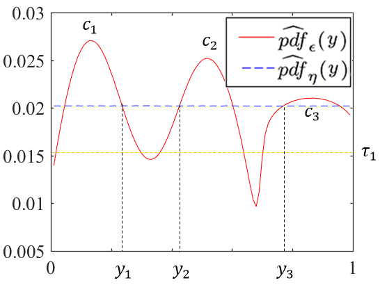
ReScale ⁴⁴ is a representative implementation algorithm based on this $cdf$ transform. Figure 2(b) and Figure 3(b) show ReScale rescales the data distribution on two 1-dimensional datasets, respectively. They show that clusters and anomalies are easier to identify after the application of ReScale.

Since this $cdf$ transform can be performed on a one-dimensional dataset only, ReScale must apply the transformation to each attribute independently for a multi-dimensional dataset.

5.2 Multi-dimensional CDF scaling

With a distance scaling method, a multi-dimensional $cdf$ transform can be achieved by simply rescaling the distances between each point and all the other instances in its local neighbourhood, (thereby considering all of the dimensions of the multi-dimensional dataset at once).

Given a point $x\in D$, the distance between $x$ and all points in its $\lambda$-neighbourhood $y\in\mathcal{N}(x;s,\lambda)$ can be rescaled using a scaling function $r(\cdot)$:

$$s^{\prime}(x,y)=s(x,y)\times r(x;\lambda),\forall_{x,y\in D,y\in\mathcal{N}(x;s,\lambda)}$$ (9)

where $s^{\prime}(\cdot,\cdot)$ is the scaled distance of $s(\cdot,\cdot)$.

Here, the scaling function $r(x;\lambda)$ depends on both the position $x$ and size of the neighbourhood $\lambda$. It is defined as follows using the estimated density $pdf(x;s,\lambda)$ with the aim of making the density distribution within the $\lambda$-neighbourhood uniform:

$$r(x;\lambda)=\frac{m}{\lambda}\times(\frac{pdf(x;s,\lambda)\times V_{\lambda}}{n})^{\frac{1}{d}}\propto pdf(x;s,\lambda)^{\frac{1}{d}}$$ (10)

where $m=max_{x,y\in D}\ s(x,y)$ is the maximum pairwise distance in $D$. Note that we have now reparameterised the density estimator $pdf(x;s,\lambda)$ to include the distance function s, in order to facilitate calculations below.

With reference to the uniform distribution which has density $\frac{n}{V_{m}}$, where $V_{m}$ is the volume of the ball having radius $m$:

$$r(x;\lambda)<1\mbox{, if }pdf(x;s,\lambda)<\frac{n}{V_{m}}$$ (11)

$$r(x;\lambda)>1\mbox{, if }pdf(x;s,\lambda)>\frac{n}{V_{m}}$$ (12)

That is, the process rescales sparse regions to be denser by using $r(x;\lambda)<1$, and dense regions to be sparser by using $r(x;\lambda)>1$; such that the entire dataset is approximately uniformly distributed in the scaled $\lambda$-neighbourhood. More specifically, after rescaling distances with s’, the density of points in the neighbourhood of size ${\lambda_{x}^{\prime}}={\lambda}\times r(x;\lambda)$ around $x$ is the same as the density of points across the whole dataset:

$${pdf}(x;s^{\prime},\lambda_{x}^{\prime})=\frac{pdf(x;s,\lambda)\times V_{\lambda}}{V_{\lambda_{x}^{\prime}}}=\frac{pdf(x;s,\lambda)\times V_{\lambda}}{V_{\lambda}\times r(x;\lambda)^{d}}$$

$$=\frac{pdf(x;s,\lambda)\times V_{\lambda}}{V_{\lambda}\times(\frac{m}{\lambda}\times(\frac{pdf(x;s,\lambda)\times V_{\lambda}}{n})^{\frac{1}{d}})^{d}}=\frac{n\times\lambda^{d}}{V_{\lambda}\times m^{d}}=\frac{n}{V_{m}}$$ (13)

Note that the above derivation is possible because (i) the scaling is isotropic about $x$ (hence the shape of the unit ball doesn’t change only its size) and (ii) the uniform-kernel density estimator is local (i.e., its value depends only on points within the $\lambda_{x}^{\prime}$ neighbourhood).

In order to maintain the same relative ordering of distances between $x$ and all other points in the dataset, the distance between $x$ and any point outside the $\lambda$-neighbourhood $y\in D\setminus\mathcal{N}(x;s,\lambda)$ can be normalised by a simple $min$-$max$ normalisation:

$$s^{\prime}({x,y})=(s({x,y})-\lambda)\times\frac{m-\lambda_{x}^{\prime}}{m-\lambda}+\lambda_{x}^{\prime},\forall_{y\in D\setminus\mathcal{N}(x;s,\lambda)}$$ (14)

The implementation of DScale ⁴⁵, which is a representative algorithm based on this multi-dimensional CDF scaling, is provided in A.

An observation about the density on the rescaled distance is given as follows:

Observation 1.

The density ${pdf}(x;s^{\prime},\gamma_{x}^{\prime})$ with the rescaled distance $s^{\prime}$ is approximately proportional to the density-ratio $\frac{pdf(x;s,\gamma)}{pdf(x;s,\lambda)}$ in terms of the original distance $s$ within the $\lambda$-neighbourhood of $x$.

Proof.

$${pdf}(x;s^{\prime},\gamma_{x}^{\prime})\approx\frac{pdf(x;s,\gamma)\times V_{\gamma}}{V_{\gamma_{x}^{\prime}}}=\frac{pdf(x;s,{\gamma})\times V_{\gamma}}{V_{\gamma}\times r(x;\lambda)^{d}}$$

$$=\frac{pdf(x;s,{\gamma})}{\frac{m^{d}}{\lambda^{d}}\times\frac{pdf(x;s,{\lambda})\times V_{\lambda}}{n}}=\frac{n}{V_{m}}\times\frac{pdf(x;s,{\gamma})}{pdf(x;s,{\lambda})}$$

$$\propto\frac{pdf(x;s,{\gamma})}{pdf(x;s,{\lambda})}$$

where ${\gamma_{x}^{\prime}}={\gamma}\times r(x;\lambda)$ and $\gamma<\lambda$. ∎

Note that the above observation is only valid within the $\lambda$-neighbourhood of $x$, and when each $x\in D$ is treated independently. In other words, the $cdf$ transform is only valid locally. In addition, the rescaled distance is asymmetric, i.e., $s^{\prime}(x,y)\neq s^{\prime}(y,x)$ when $r(x;\lambda)\neq r(y;\lambda)$.

To be a valid $cdf$ transform globally for the entire dataset, we propose in this paper to perform an iterative process that involves two steps: distance rescaling and point shifting.

6 CDF Transform-and-Shift

Here we present our proposed method, which we call CDF Transform-and-Shift (CDF-TS) because the key process is motivated by and based on a multi-dimensional CDF scaling.

A CDF transform on a dataset produces a uniformly distributed dataset ³⁵. However, an entire dataset of a single uniform distribution destroys the cluster structures in the dataset which is of no use for data mining.

The proposed method aims to reduce the density variation of a given dataset, effectively equalises the density of all clusters (of high-density regions) as well as equalises the density of low-density regions (between any two clusters). The latter ensures that the cluster structure in the dataset is preserved; while the former conforms to the implicit assumption of existing density-based algorithms. These enable each of the existing algorithms to identify all clusters that would be otherwise impossible.

This is achieved through a CDF transform-and-shift process. While the same CDF transform process as DScale is used, the additional “shift” ensures that (i) the transformed-and-shifted dataset becomes approximately uniformly distributed in the scaled $\lambda$-neighbourhood; and (ii) the standard Euclidean distance can then be used to measure distances between any two transformed-and-shifted points. These advantages are not available in DScale which relies on a rescaled distance which is non-metric and asymmetric.

The CDF transform-and-shift process is described as follows.

Consider two points $x,y\in D$. In order to make the distribution around point $x$ more uniform, we wish to rescale (expand or contract) the distance between $x$ and $y$ to be $s^{\prime}(x,y)$ as defined by Equations 9 and 14. We do this by translating $y$ to a new point denoted $y_{x}^{\prime}$ which lies along the direction $(y-x)$ as follows:

$$y_{x}^{\prime}=x+\frac{s^{\prime}(x,y)}{s(x,y)}(y-x)$$ (15)

Note that the distance between $x$ and the newly transformed point $y_{x}^{\prime}$ satisfies the rescaled distance requirement:

$$s(x,y_{x}^{\prime})=||y_{x}^{\prime}-x||=\frac{s^{\prime}(x,y)}{s(x,y)}||(y-x)||=s^{\prime}(x,y)$$ (16)

So far we have considered the effect of translating point $y$ to $y_{x}^{\prime}$ wtih respect to $x$ only. To consider the effects with respect to all points $D$, point $y$ needs to be transformed by the average of the above translations with respect to all points in $D$:

$$\bar{y}^{\prime}=\frac{1}{n}\sum_{x\in D}y_{x}^{\prime}=\frac{1}{n}\sum_{x\in D}\left[x+\frac{s^{\prime}(x,y)}{s(x,y)}(y-x)\right]$$ (17)

We make the following observation regarding the final shifted dataset, denoted $D^{\prime}=\{\bar{y}^{\prime}|y\in D\}$:

Observation 2.

Given a dataset, if there is a sufficiently small bandwidth $\lambda\!<\!m$ such that for every point $x\!\in\!D$ the density over its neighbourhood $\mathcal{N}(x;s,\lambda)$ varies relatively slowly, then the variance in $\lambda$-neighbourhood density should reduce as a result of the data transformation, i.e.:

$$\mathbb{VAR}_{\bar{x}^{\prime}\in D^{\prime}}[pdf(\bar{x}^{\prime};s,\lambda)]<\mathbb{VAR}_{x\in D}[pdf(x;s,\lambda)]$$ (18)

We provide an intuitive argument supporting this observation in B.

Furthermore, the transform-and-shift process can be repeated multiple times iteratively to further reduce the variance in the $\lambda$-neighbourhood density estimates.

Although CDF-TS takes the average of scaling effects from all data points, the $\lambda$-neighbourhood densities of all points approximate to be uniformly distributed. Since Equations 15 and 17 are based on the linear transformation within and outside the $\lambda$-neighbourhood of a data point, the local density-variation inside the $\lambda$-neighbourhood can be preserved in each shift process, i.e., the locally low-density gaps between clusters become globally low-density gap, as shown in Observation 1.

The key parameter $\lambda$ is very important for this shift process. In case a non-convergence situation arises from an inappropriate $\lambda$ setting, we set a condition where the iteration process stops: when a fixed iteration limit is reached, or when the total movement of points between iterations ($D$ to $D^{\prime}$) falls below a threshold $\delta$. Here we use a Manhattan distance to measure the movement in our experiments, i.e.,

$$\sum_{x\in D,\ \bar{x}^{\prime}\in D^{\prime}}{|x-\bar{x}^{\prime}|}\leq\delta$$ (19)

Figure 4 illustrates the effects of CDF-TS on a two-dimensional dataset with different iterations. It shows that the original clusters with different densities become increasing uniform with less density variation as the number of iterations increases. In addition, the gaps between different clusters become more obvious after iterations.

(a) A two-dimensional data with $Std(x)=4.29$

(b) After 1 iteration $Std(x)=1.65$

(c) After 3 iterations $Std(x)=0.62$

(d) After 5 iterations $Std(x)=0.42$

Figure 4: Scatter plots for illustrating the effects of CDF-TS on a two-dimensional data with $\lambda=0.1$. $Std(x)=\sigma(\widehat{pdf}_{\epsilon}(x\in D))$ represents the standard deviation of the density with $\epsilon=0.1$.

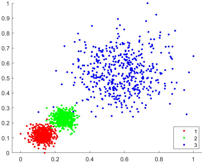
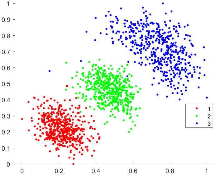
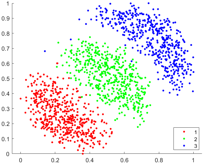
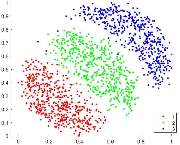
The implementation of CDF-TS is shown in Algorithm 1. The DScale algorithm used in step 6 is provided in A. Algorithm 1 requires two parameters $\lambda$ and $\delta$. Note that, due to the shifts in each iteration, the value ranges of attributes of the shifted dataset $D^{\prime}$ are likely to be different from those of the original dataset $D$. We can use a min-max normalisation ³ on each attribute to keep the values in the same fixed range at the end of each iteration. In addition, we set the maximum number of iterations to prevent the unconverged situation.

Algorithm 1 CDF-TS($D$, $\lambda$, $\delta$)

1:$D$ - input data matrix ($n\times d$ matrix); $\lambda$ - bandwidth parameter; $\delta$ - threshold for the total shifted distance.

2:$D^{\prime}$ - data matrix after rescaling and point shifting.

3:Normalising $D$ using min-max normalisation

4:$\Delta=\infty$

5:$t=1$

6:while $\Delta>\delta$ and $t<100$ do

7:     $S\leftarrow$ Calculating the distance matrix for $D$

8:     $S^{\prime}\leftarrow$ DScale($S$, $\lambda$, $d$)

9:     for each $z\in D$ (where $z$ is a reference point) do

10:         $D_{z}\leftarrow$ Shift every point $x\in D$ to $x_{z}^{\prime}$ in the direction of $z$ to $x$ with magnitude $S^{\prime}[z,x]$

11:     end for

12:     $D^{\prime}\leftarrow\frac{1}{n}\sum_{z\in D}D_{z}$

13:     Normalising $D^{\prime}$ using min-max normalisation

14:     $\Delta=\frac{1}{nd}\sum_{i,j}|D[i,j]-D^{\prime}[i,j]|$

15:     $t=t+1$

16:     $D=D^{\prime}$

17:end while

18:return $D^{\prime}$

To demonstrate the effects of different density-ratio based rescaling methods (ReScale ⁴⁴, DScale ⁴⁵ and CDF-TS), we apply them for the same image segmentation task as shown in Table 1. Table 2 shows the results of applying the clustering algorithm DP ³⁴ to produce three clusters on the image shown in Figure 1. The scatter plots in LAB space in Table 2 show that the three clusters become more homogeneous distributed. Although the density variation of CDF-TS is not the smallest, the gaps between cluster boundaries are much larger for CDF-TS than the other scaling methods. Thus, DP with CDF-TS yields the best clustering result, shown in Table 2. This also shows that density equalisation is not the only aim; and by itself, density equalisation does not achieve the intended outcome of identifying all clusters in the dataset.

Table 2: DP’s image segmentation on the image shown in Figure 1. The colours in the scatter plots indicate the three clusters identified by DP using each of the four methods. The scatter plots of DScale and No Scaling are based on the original LAB attributes; and the other two are based on the transformed attributes. Note that the standard deviation of the density distribution of points in the LAB space are 12.82, 7.03, 3.19 and 7.85 for the four sub-figures, respectively. The density estimation is based on Equation 1 with $\epsilon=0.1$.

	LAB	Cluster 1	Cluster 2	Cluster 3
No Scaling
ReScale
DScale
CDF-TS

6.1 Density estimators applicable to CDF-TS

The following two types of density estimators, with fixed-size and variable-size bandwidths of the uniform kernel, are applicable to CDF-TS to do the CDF scaling:

(a) $\epsilon$-neighbourhood density estimator:

$$\widehat{pdf}_{\epsilon}(x)=\frac{|\{y\in D\leavevmode\nobreak\ |\leavevmode\nobreak\ s(x,y)\leqslant\epsilon\}|}{nV_{\epsilon}}$$

where $V_{\epsilon}$ is the volume of the ball with radius $\epsilon$.

When this density estimator is used in CDF-TS, the $\lambda$-neighbourhood described in Sections 5.2 and 6, i.e., $\mathcal{N}(x;s,\lambda)=\{y\in D\leavevmode\nobreak\ |\leavevmode\nobreak\ s(x,y)\leqslant\epsilon\}$, where $\lambda=\epsilon$, denoting the fixed-size bandwidth uniform kernel.

(b) $k$-th nearest neighbour density estimator:

$$\widehat{pdf}(x;\epsilon_{k}(x))=\frac{k}{nV_{s(x,x_{k})}}\propto(\frac{1}{s(x,x_{k})})^{d}$$

where $x_{k}$ is the $k$-th nearest neighbour of $x$; $\epsilon_{k}(x)$ is $k$-th nearest neighbour distance of $x$.

When this density estimator is used in CDF-TS, the neighbourhood size $\lambda$ becomes dependent on the location $x$ and the distribution of surrounding points. We denote $\lambda(x)_{k}=s(x,x_{k})$ as the distance to the $k$-th nearest neighbour of $x$. In this case the density is simply calculated over the neighbourhood: $\mathcal{N}(x;s,\lambda(x)_{k})=\{y\in D\leavevmode\nobreak\ |\leavevmode\nobreak\ s(x,y)\leqslant s(x,x_{k})\}$, denoting the variable-size bandwidth uniform kernel, i.e., small in dense region and large in sparse region. Note that, in this circumstance, the density of each shifted point also becomes more uniform w.r.t their surrounding.

In the following experiments, we employ the same density estimators used in DBSCAN and DP (in clustering) and $k$NN anomaly detector in CDF-TS to transform $D$ to $D^{\prime}$, i.e., $\epsilon$-neighbourhood density estimator is used in CDF-TS for clustering; and $k$-th nearest neighbour density estimator is used in CDF-TS for anomaly detection.

7 Empirical Evaluation

This section presents experiments designed to evaluate the effectiveness of CDF-TS.

All algorithms used in our experiments were implemented in Matlab R2020a (the CDF-TS source code is available at https://sourceforge.net/p/cdf-ts/). The experiments were run on a machine with eight cores CPU (Intel Core i7-7820X @ 3.60GHz), 32GB memory and a 2560 CUDA cores GPU (GeForce GTX 1080). All datasets were normalised using the $min$-$max$ normalisation to yield each attribute to be in [0,1] before the experiments began.

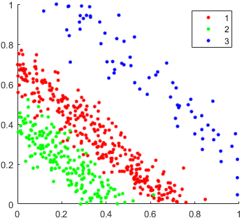
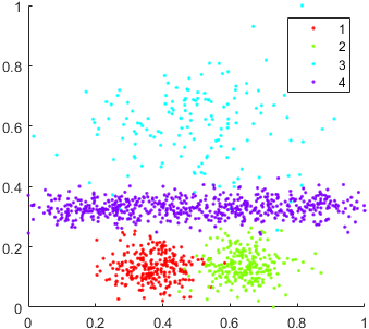
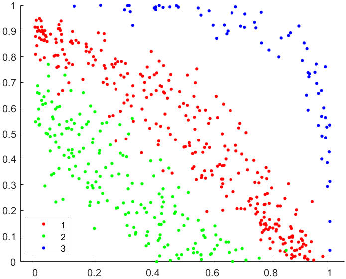
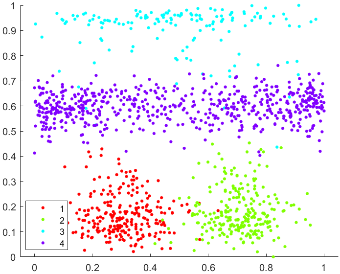
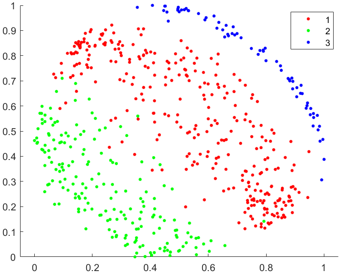
For clustering, we used two artificial datasets and 13 real-world datasets with different data sizes and dimensions from the UCI Machine Learning Repository ¹⁴. Table 3 presents the data properties of the datasets. 3L is a 2-dimensional data containing three elongated clusters with different densities, as shown in Figure 5(a). 4C dataset is a 2-dimensional dataset containing four clusters with different densities (three Gaussian clusters and one elongated cluster), as shown in Figure 5(b). Note that DBSCAN is unable to correctly identify all clusters in both of these datasets because they do not satisfy the condition specified in Equation 2. Furthermore, clusters in 3L dataset significantly overlap on individual attribute projections, which violates the requirement of ReScale that one-dimensional projections allow for the identification of the density peaks of each cluster.

Table 3: Properties of datasets used for clustering

Dataset	Data Size	#Dimensions	#Clusters
Pendig	10992	16	10
Segment	2310	19	7
Mice	1080	83	8
Biodeg	1055	41	2
ILPD	579	9	2
ForestType	523	27	4
Wilt	500	5	2
Musk	476	166	2
Libras	360	90	15
Dermatology	358	34	6
Haberman	306	3	2
Seeds	210	7	3
Wine	178	13	3
3L	560	2	3
4C	1250	2	4

(a) 3L data distribution

(b) 4C data distribution

Figure 5: (a) The scatter plot of a two-dimensional data containing three elongated clusters. (b) The scatter plot of a two-dimensional data containing four clusters.

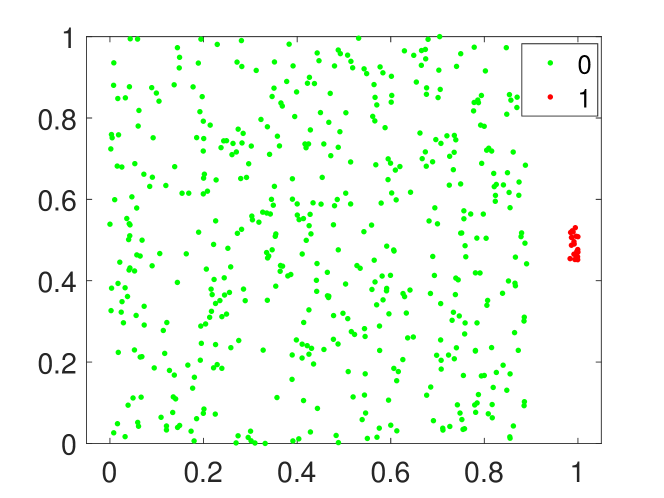
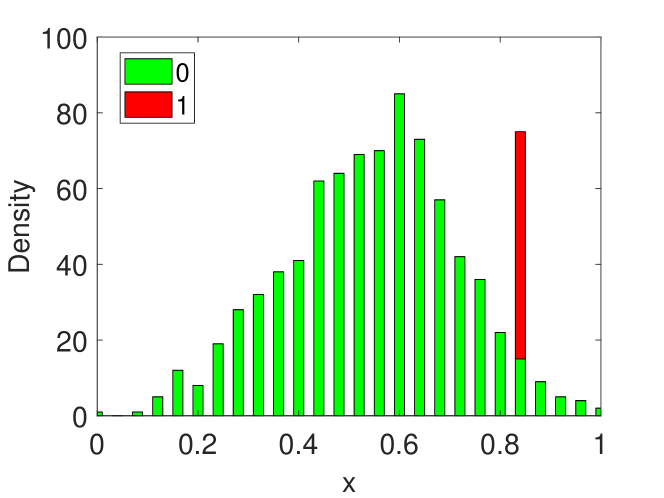
For anomaly detection, we compared the anomaly detection performance on two synthetic datasets with anomalous clusters and 10 real-world benchmark datasets. The data size, dimensions and percentage of anomalies are shown in Table 4. Both the Syn 1 and Syn 2 datasets contain clusters of anomalies. Their data distributions are shown in Figure 6.

Table 4: Properties of datasets used for anomaly detection

Dataset	Data Size	#Dimensions	% Anomaly
AnnThyroid	7200	6	7.4%
Pageblocks	5473	10	10.2%
Tomcat	858	20	9.0%
Ant	745	20	22.3%
BloodDonation	604	4	5.6%
Vowel	528	10	9.1%
Mfeat	410	649	2.4%
Dermatology	358	34	5.6%
Balance	302	4	4.6%
Velocity	229	20	34.1%
Syn 1	520	2	3.9%
Syn 2	860	1	7.0%

(a) The scatter plot of Syn 1 dataset

(b) The stacked histogram on Syn 2 dataset

Figure 6: Data distributions of the Syn 1 and Syn 2 datasets, where the red colour indicates the anomaly.

7.1 Clustering

In this section, we compare CDF-TS with ReScale and DScale using four existing density-based clustering algorithms, i.e., DBSCAN ¹⁶, DP ³⁴ , LGD ²³ and EC ⁴³, in terms of F-measure ³³: given a clustering result, we calculate the precision score $P_{i}$ and the recall score $R_{i}$ for each cluster $C_{i}$ based on the confusion matrix, and then the F-measure score of $C_{i}$ is the harmonic mean of $P_{i}$ and $R_{i}$. The overall F-measure score is the unweighted (macro) average over all clusters: F-measure$=\frac{1}{\varsigma}\sum_{i=1}^{\varsigma}\frac{2P_{i}R_{i}}{P_{i}+R_{i}}$.

We report the best clustering performance after a parameter search for each algorithm. Table 5 lists the parameters and their search ranges for each algorithm. $\psi$ in ReScale controls the precision of $\widehat{cdf}_{\lambda}(x)$, i.e., the number of intervals used for estimating $\widehat{cdf}_{\lambda}(x)$. We set $\delta=0.015$ as the default value for CDF-TS.

Table 5: Parameters and their search ranges. The search ranges of $\psi$ and $\lambda$ are as used by Zhu et. al. ⁴⁴. The parameter search ranges for LGD follow the original paper ²³

. Algorithm Parameters with search ranges DBSCAN $Minpts\in\{2,3,...,10\}$; $\epsilon\in[0,1]$ DP $k\in\{2,3,...,20\}$; $\epsilon\in[0,1]$ EC $\epsilon\in[0,1]$ LGD $k\in\{2,4,6,10,15,20\}$; $\tau\in[0.5,0.52,0.56,0.62]$; $c=\#clusters$ ReScale $\psi=100$; $\lambda\in\{0.1,0.2,...,0.5\}$ DScale $\lambda\in\{0.1,0.2,...,0.5\}$ CDF-TS $\lambda\in\{0.1,0.2,...,0.5\}$; $\delta=0.015$

Table 6 shows the best F-measures for DBSCAN, DP, EC, LGD and their ReScale, DScale and CDF-TS versions. The average F-measures, showed in the second last row, reveal that CDF-TS improves the clustering performance of all clustering algorithms with a larger performance gap than both ReScale and DScale. In addition, CDF-TS is the best performer on many more datasets than other contenders (shown in the last row of Table 6.)

Table 6: The best F-measure for DBSCAN, DP, EC, LGD and their ReScale, DScale and CDF-TS versions. For each clustering algorithm, the best performer in each dataset is boldfaced. Ori, ReS, and DS represent the Original algorithm, ReScale, and DScale respectively.

Data	DBSCAN				DP				EC				LGD
	Orig	ReS	DS	CDF-TS	Orig	ReS	DS	CDF-TS	Orig	ReS	DS	CDF-TS	Orig	ReS	DS	CDF-TS
Pendig	0.70	0.78	0.74	0.80	0.79	0.82	0.82	0.84	0.79	0.84	0.84	0.844	0.83	0.878	0.87	0.88
Segment	0.59	0.62	0.61	0.67	0.78	0.77	0.80	0.84	0.57	0.66	0.69	0.66	0.76	0.73	0.76	0.80
Mice	0.99	0.99	0.99	0.993	1.00	1.00	1.00	1.00	0.98	0.98	0.99	0.99	1.00	1.00	1.00	1.00
Biodeg	0.45	0.44	0.47	0.52	0.72	0.74	0.73	0.76	0.45	0.44	0.61	0.70	0.68	0.70	0.71	0.73
ILPD	0.41	0.42	0.56	0.52	0.60	0.63	0.62	0.64	0.49	0.49	0.58	0.57	0.57	0.62	0.57	0.600
ForestType	0.27	0.51	0.48	0.65	0.69	0.83	0.70	0.85	0.28	0.66	0.55	0.84	0.63	0.82	0.80	0.84
Wilt	0.38	0.39	0.54	0.55	0.54	0.68	0.54	0.74	0.44	0.53	0.49	0.67	0.53	0.56	0.54	0.71
Musk	0.51	0.52	0.51	0.53	0.55	0.58	0.61	0.62	0.51	0.53	0.54	0.53	0.60	0.61	0.63	0.586
Libras	0.41	0.44	0.46	0.49	0.52	0.52	0.52	0.53	0.46	0.46	0.49	0.49	0.48	0.51	0.49	0.54
Dermatology	0.52	0.73	0.74	0.83	0.91	0.97	0.91	0.96	0.73	0.76	0.75	0.87	0.92	0.97	0.94	0.96
Haberman	0.47	0.64	0.59	0.66	0.56	0.63	0.58	0.67	0.49	0.58	0.54	0.66	0.53	0.67	0.56	0.664
Seeds	0.75	0.88	0.85	0.83	0.91	0.92	0.92	0.94	0.90	0.90	0.91	0.88	0.91	0.91	0.91	0.91
Wine	0.64	0.86	0.80	0.90	0.93	0.95	0.96	0.962	0.84	0.92	0.90	0.88	0.92	0.94	0.92	0.96
3L	0.59	0.63	0.90	0.88	0.82	0.81	0.86	0.89	0.76	0.79	0.70	0.73	0.71	0.71	0.71	0.70
4C	0.71	0.90	0.92	0.95	0.87	0.92	0.95	0.91	0.86	0.88	0.88	0.883	0.95	0.961	0.95	0.96
Average	0.56	0.65	0.68	0.72	0.75	0.78	0.77	0.81	0.64	0.70	0.70	0.75	0.73	0.77	0.76	0.79
#Top 1	0	1	2	12	1	2	2	13	0	2	3	11	1	4	1	12

It is interesting to see that CDF-TS performs notably better than both DBSCAN and DP on many datasets, such as ForestType, Wilt, Dermatology and Wine. On most datasets, CDF-TS also outperforms its competitors ReScale and/or DScale by a wide gap.

Note that the performance gap is smaller for DP than it is for DBSCAN because DP is a more powerful algorithm which does not rely on a single density threshold to identify clusters.

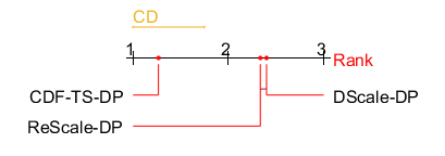
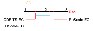
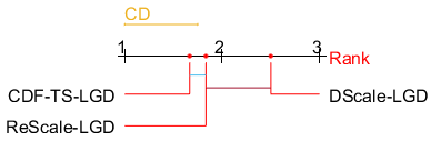
To evaluate whether the performance difference among the three scaling algorithms is significant, we conduct the Friedman test with the post-hoc Nemenyi test ¹³. Figure 7 shows the results of the significance test for different clustering algorithms. The results show that the CDF-TS versions are significantly better than at least one of DScale and ReScale versions for each clustering algorithm.

(a) Significance test for DBSCAN

(b) Significance test for DP

(c) Significance test for EC

(d) Significance test for LGD

Figure 7: Critical difference (CD) diagram of the post-hoc Nemenyi test ($\alpha=0.10$). Two algorithms are significantly different if the gap between their ranks is larger than the CD. Otherwise, there is a line linking them.

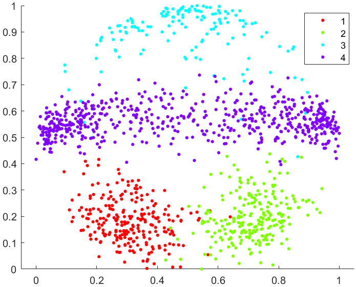
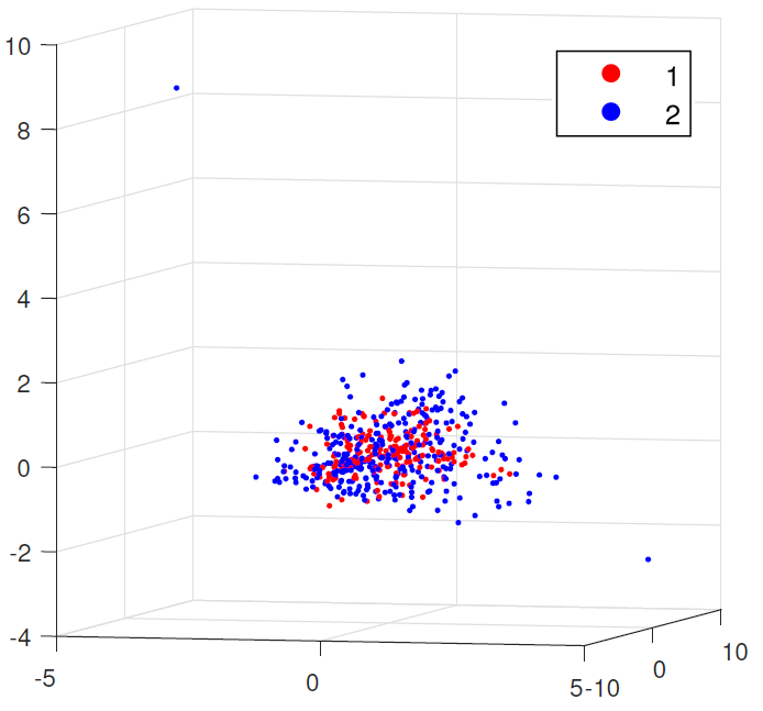
Here we compare the different effects on the transformed datasets due to ReScale and CDF-TS. The effects on the two synthetic datasets are shown in Figure 8 and Figure 10. They show that both the rescaled datasets are more axis-parallel distributed using ReScale than those using CDF-TS. For the 3L dataset, the blue cluster is still very sparse after running ReScale, as shown in Figure 8(a). In contrast, it becomes denser using CDF-TS, as shown in Figure 9(a). As a result, DBSCAN has much better performance with CDF-TS on the 3L dataset. Figure 10 shows the MDS visualisation on the Wilt dataset where CDT-TS outperforms both DBSCAN and DP the most. The figure shows that the each cluster is more homogeneously distributed in the new space, which makes the boundary between clusters easier to be identified than that in the original space. In contrast, based on distance, most points of the red cluster are surrounded by points of the blue cluster, as shown in Figure 9(c).

(a) 3L data distribution

(b) 4C data distribution

Figure 8: Scatter plots after running ReScale when achieving the best DBSCAN clustering performance

(a) 3L data distribution

(b) 4C data distribution

Figure 9: Scatter plots after running CDF-TS when achieving the best DBSCAN clustering performance

(c) Based on distance

(d) Based on CDF-TS

Figure 10: MDS plots on the Wilt dataset

7.2 Anomaly detection

In this section, we evaluate the ability of CDF-TS to detect local anomalies based on $k$NN anomaly detection.

Three state-of-the-art anomaly detectors, Local Outlier Factor (LOF) ⁹, iForest ²⁴ and iNNE ⁶, are also used in the comparison. Table 7 lists the parameters and their search ranges for each algorithm. Parameters $\psi$ and $t$ in iForest control the sub-sample size and number of iTrees, respectively. We report the best performance of each algorithm on each dataset in terms of best AUC (Area under the Curve of ROC) ¹⁸.

Table 7: Parameters and their search ranges.

Algorithm	Parameters and their search ranges
$k$NN/LOF	$k\in\{5\%n,10\%n,...,50\%n\}$
iForest/iNNE	$t=100$; $\psi\in\{2^{1},2^{2},...,2^{10}\}$
ReScale	$\psi=100$; $\lambda\in\{0.1,0.2,...,0.5\}$
DScale	$\lambda\in\{0.1,0.2,...,0.5\}$
CDF-TS	$\lambda\in\{0.1,0.2,...,0.5\}$; $\delta=0.015$

Table 8 compares the best AUC score of each algorithm. CDF-TS-$k$NN achieves the highest average AUC of 0.90 and performs the best on 5 out of 12 datasets. For the Syn 1 dataset which has significant overlapping on the individual attribute projection, iForest and ReScale perform the worst because they are based on individual attribute splitting and scaling, respectively. All of ReScale, DScale and CDF-TS improve the performance of $k$NN on Syn 1 dataset which has cluster anomalies, because these anomalies become farther from the normal cluster centre. It is interesting to mention that CDF-TS-$k$NN has the largest AUC increase in $k$NN on Dermatology and AnnThyroid.

Table 8: The best AUC on 12 datasets. The best performer on each dataset is boldfaced. Original, ReScale, DScale and CDF-TS represent $k$NN, ReScale-$k$NN, DeScale-$k$NN and CDF-TS-$k$NN, respectively.

Data	LOF	iForest	iNNE	$k$NN
				Original	ReScale	DScale	CDF-TS
AnnThyroid	0.68	0.88	0.74	0.65	0.76	0.71	0.94
Pageblocks	0.93	0.90	0.92	0.89	0.88	0.86	0.94
Tomcat	0.67	0.81	0.69	0.63	0.77	0.69	0.78
Ant	0.68	0.77	0.70	0.67	0.76	0.71	0.76
BloodDonation	0.79	0.82	0.74	0.69	0.84	0.80	0.86
Vowel	0.93	0.92	0.95	0.93	0.930	0.90	0.94
Mfeat	0.98	0.98	0.99	0.99	0.99	1.00	0.99
Dermatology	0.99	0.86	0.98	0.91	0.99	0.97	1.00
Balance	0.95	0.91	0.97	0.94	0.91	0.83	0.92
Velocity	0.62	0.65	0.61	0.66	0.67	0.694	0.69
Syn 1	0.93	0.90	0.94	0.92	0.89	0.95	0.98
Syn 2	0.88	0.86	0.91	0.88	0.92	0.95	0.94
Average	0.83	0.86	0.85	0.81	0.86	0.84	0.90
#Top 1	0	2	2	0	0	3	5

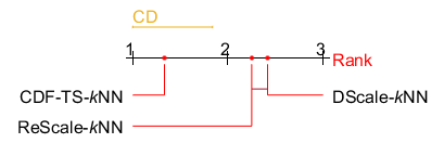
Figure 11 shows the significance test on the three algorithms applied to $k$NN anomaly detector. It can be seen from the results that CDF-TS-$k$NN is significantly better than DScale-$k$NN and ReScale-$k$NN.

Figure 11: Critical difference (CD) diagram of the post-hoc Nemenyi test ($\alpha=0.10$) for anomaly detection algorithms.

7.3 Compared with metric learning algorithms

We have examined the best performance of PCA ²¹ and t-SNE ²⁷ in DP clustering and $k$NN anomaly detection, as shown in Table 9 and Table 10, respectively. We set the dimensionality of PCA and t-SNE output space to 2 or $d$. The perplexity in t-SNE are searched in $[10,20,30,40,50]$. We find that PCA could not improve the performance on most of these tasks. t-SNE-DP has comparable clustering performance to CDF-TS-DP. However, t-SNE could not improve the performance on $k$NN anomaly detector on some datasets, such as the AnnThyroid, Pageblocks and Tomcat datasets.

Table 9: The best F-measure of DP and its PCA, t-SNE and CDF-TS versions. For each version, the best performer in each dataset is boldfaced.

Dataset	DP
	Original	PCA	t-SNE	CDF-TS
Segment	0.78	0.78	0.81	0.84
Mice	1.00	1.00	1.00	1.00
Biodeg	0.72	0.72	0.73	0.76
ILPD	0.60	0.60	0.61	0.64
ForestType	0.69	0.75	0.87	0.85
Wilt	0.54	0.55	0.60	0.74
Musk	0.55	0.55	0.58	0.62
Libras	0.52	0.52	0.56	0.53
Dermatology	0.91	0.91	0.97	0.96
Haberman	0.56	0.56	0.57	0.67
Seeds	0.91	0.93	0.94	0.94
Wine	0.93	0.98	0.97	0.96
3L	0.82	0.70	0.91	0.89
4C	0.87	0.87	0.96	0.91
Average	0.74	0.74	0.79	0.81
#Top 1	1	2	7	8

Table 10: The best AUC on 12 datasets. The best performer on each dataset is boldfaced. PCA, t-SNE and CDF-TS represent PCA-$k$NN, t-SNE-$k$NN and CDF-TS-$k$NN, respectively.

Data	$k$NN
	Original	PCA	t-SNE	CDF-TS
AnnThyroid	0.65	0.65	0.67	0.94
Pageblocks	0.89	0.89	0.88	0.94
Tomcat	0.63	0.63	0.60	0.78
Ant	0.67	0.67	0.68	0.76
BloodDonation	0.69	0.75	0.75	0.86
Vowel	0.93	0.93	0.97	0.94
Mfeat	0.99	0.99	1.00	0.99
Dermatology	0.91	0.91	1.00	1.00
Balance	0.94	0.96	0.94	0.92
Velocity	0.66	0.66	0.67	0.69
Syn 1	0.92	0.92	1.00	0.98
Syn 2	0.88	0.88	0.96	0.94
Average	0.81	0.82	0.84	0.90
#Top 1	0	1	5	7

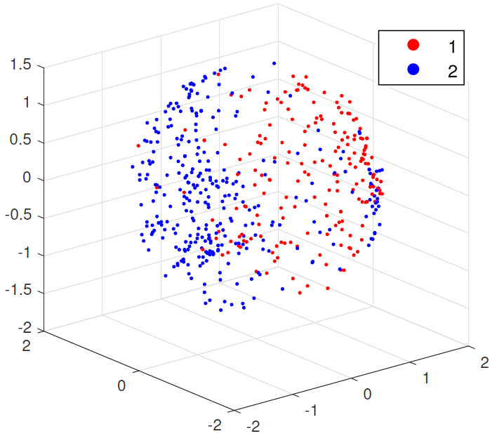
In order to visually compare the effects of these transform methods, Table 11 shows the visualisation results on two datasets. It shows that most anomalies become anomalous clusters and farther away from normal points on the CDF-TS transformed datasets, and thus easier to be detected by the $k$NN anomaly detector. When using PCA, some normal points are still scattered having a large $k$NN distance from other normal points on the Dermatology dataset, so it has the same AUC score to that obtained on the original dataset. On the AnnThyroid dataset, the clustered anomalies are still close to normal clusters in the t-SNE transformed space. With CDF-TS, the normal points occur on a sphere and there is a large gap between the surface of the sphere and the anomalies.

Table 11: Visualisation results on two datasets, where red points indicate anomalies. Distance and CDF-TS results are based on MDS, $\eta=0.1$ and $\delta=0.015$ in CDF-TS; PCA and t-SNE results set output dimensionality to 3, and perplexity in t-SNE is 30.

	Distance	PCA	t-SNE	CDF-TS
Dermatology
AnnThyroid

7.4 Run-time

ReScale, DScale, PCA, t-SNE and CDF-TS are all pre-processing methods, their computational complexities are shown in Table 12. Because many existing density-based clustering algorithms have time and space complexities of $\mathcal{O}(n^{2})$, all these methods do not increase their overall complexities.

Table 12: Computational complexity of ReScale, DScale, PCA, t-SNE and CDF-TS.

Algorithm	Time complexity	Space complexity
PCA	$\mathcal{O}(dn^{2}+d^{3})$	$\mathcal{O}(dn)$
t-SNE	$\mathcal{O}(dn^{2})$	$\mathcal{O}(n^{2})$
ReScale	$\mathcal{O}(dn\psi)$	$\mathcal{O}(dn+d\psi)$
DScale and CDF-TS	$\mathcal{O}(dn^{2})$	$\mathcal{O}(dn+n^{2})$

Table 13 shows the runtime of the dissimilarity matrix calculation for each of the three methods on the Mfeat, Segment, Pageblocks and AnnThyroid datasets. Their parameters are set to be the same for all datasets, i.e., $\lambda=0.2$, $\psi=100$, $perplexity=30$, $NumDimensions=2$ and $\delta=0.015$. The result shows that CDF-TS had longer runtime than DScale because it requires multiple DScale calculations. However, t-SNE took the longest runtime because of search and optimisation algorithms used. We omit GPU results of PCA and t-SNE because their available program cannot take the advantage of GPU on the Matlab platform.

Table 13: Runtime comparison of dissimilarity matrix calculation (in seconds).

Dataset	CPU					GPU
	ReScale	DScale	PCA	t-SNE	CDF-TS	ReScale	DScale	CDF-TS
Mfeat	0.69	0.03	0.05	2.47	1.26	0.05	0.02	2.89
Segment	0.29	0.28	0.01	23.38	2.68	0.02	0.05	0.11
Pageblocks	0.16	1.64	0.01	43.71	18.64	0.02	0.17	2.84
AnnThyroid	0.19	3.09	0.01	61.52	24.40	0.02	0.26	2.97

8 Discussion

8.1 Parameter settings

Both DScale and CDF-TS are preprocessing methods and have one critical parameter $\lambda$ to define the $\lambda$-neighbourhood. The density-ratio based on a small $\lambda$ will approximate density ratio of 1 everywhere and provides no information; while on a large $\lambda$, it will approximate the actual density and has no advantage. Generally, in practice, we found that $\lambda\in[0.1,0.3]$ and $\epsilon$ in DBSCAN and DP shall be set slightly smaller than $\lambda$. The $\lambda$ could be larger for high-dimensional and sparse datasets to include sufficient points in the $\lambda$-neighbourhood.

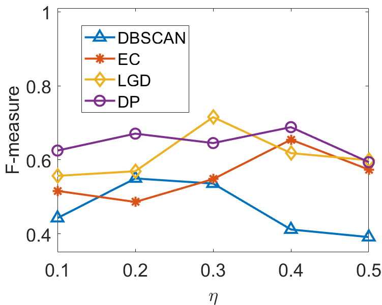
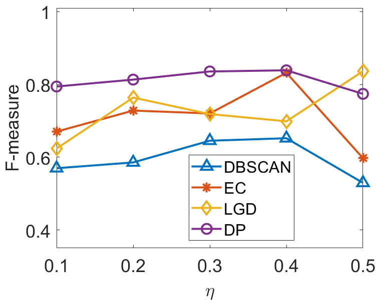
The parameter $\delta$ in CDF-TS controls the number of iterations, i.e., a small $\delta$ usually results in a high number of iterations in the CDF-TS process, which yields the desired outcome: the shifted clusters of homogeneous density. In our experiments, we set $\delta=0.015$ as the default value which usually ran in about 5 iterations in CDF-TS. This significantly improves the clustering results of existing algorithms. We provide a sensitivity test about $\eta$ and the number of iterations for CDF-TS on four datasets in D.

Since CDF-TS is a preprocessing technique, we have used clustering and anomaly detection algorithms to indirectly validate the effectiveness of the transformation, i.e., it can improve the task-specific performance of existing clustering and anomaly detection algorithms.

However, existing density-based algorithms are sensitive to parameter settings and there is no uniform guide in setting their parameters. The sensitivity exists because the nonparametric density estimator used in these algorithms suffers from noise in a random sample without specific knowledge about the data domain ¹⁹. Although there are some heuristic methods, their performance cannot be guaranteed.

Hyperparameter optimisation in a clustering algorithm, as an unsupervised learning method, is still an open question in the research community and is beyond the scope of this paper ². We followed the common practice in searching the best parameters for each algorithm to demonstrate its optimal performance.

In addition, we used a train-and-test evaluation method to compare the performance of t-SNE and CDF-TS, where a dataset is split into two subsets of equal size and the parameter setting of an algorithm is determined on the training set before it is used on the test. The results show that CDF-TS still performs better than t-SNE on $k$NN anomaly detection tasks, i.e., CDF-TS has an average AUC of 0.90 and t-SNE has an average AUC of 0.82 with $k$NN anomaly detector. However, since density-based clustering is very sensitive to the data sampling variation, both CDF-TS and t-SNE only get the average F-measure of 0.65 with DP, still better than the original DP with the average F-measure of 0.62.

8.2 Compared with a density equalisation method

CDF-TS reduces density variance of the dataset, such that the cluster structure becomes clearer and easier to be extracted with a single density threshold. If the density is equalised irrespective of the bandwidth selection, then the cluster density information will be totally lost; and there will be no clusters to detect.

In the context of kernel $k$-means, $k$NN kernel ²⁸ has been suggested to be a way to equalise the density of a given dataset to reduce the bias of kernel $k$-means algorithm and to improve the clustering performance on datasets with inhomogeneous cluster densities. The dissimilarity matrix generated by $k$NN kernel is binary. It can be seen as the adjacent matrix of $k$NN graph such that “1” means a point is in the set of $k$ nearest neighbours of another point, and “0” otherwise. Thus, a $k$-means clustering algorithm can be used to group points based on their $k$NN graph.

However, $k$NN kernel cannot be applied to both density-based clustering and $k$NN anomaly detection. This is because it converts all points to have the same density in the new space regardless of a density estimator (and its bandwidth setting) used in an intended algorithm. Thus, DBSCAN will either group neighbouring clusters into a single cluster or assign all clusters to noise.

kNN kernel doesn’t work for DP either for the same reason DP links a point to another point with a higher density to form clusters in the last step of the clustering process ³⁴. DP would not be able to link points when all points have the same density.

For $k$NN anomaly detection, replacing the distance measure with the $k$NN kernel produces either 0 or 1 similarity between any two points. This does not work for anomaly detection.

9 Conclusions

The density bias issue has been a perennial problem for existing density-based algorithms. Different methods have been attempted, but the issue remains.

We introduce a CDF Transform-and-Shift (CDF-TS) algorithm to comprehensively address this issue for both density-based clustering and distance-based anomaly detection algorithms. This is achieved without substantial computational cost. As CDF-TS is applied as a preprocessing step, no algorithmic modification is required to these algorithms to address their density bias issue.

CDF-TS is the first density-ratio method that performs both the space transformation and point-shift comprehensively, i.e., (a) all locally low-density locations in the original space become globally low-density locations in the transformed space; and (b) the volume of every point’s neighbourhood in the entire multi-dimensional space is modified via point-shifting in order to homogenise cluster density. Existing CDF transform methods such as ReScale ⁴⁴ and DScale ⁴⁵ achieve a much-reduced effect on the rescaled dataset because the former is a one-dimensional method and the latter is one without point-shifting (and the resultant measure is not a metric).

In addition, CDF-TS is more generic than these two CDF transform methods because the algorithm permits different density estimators. We show that either $\epsilon$-neighbourhood or $k$NN density estimators can be successfully incorporated. It is also more effective than existing methods such as t-SNE and $k$NN kernel ²⁸. As a result, CDF-TS can be applied to more algorithms/tasks with a better outcome than these methods.

Through extensive evaluations, we show that CDF-TS significantly improves the performance of four existing density-based clustering algorithms and one existing distance-based anomaly detector.

It is interesting to note that other algorithms, which are not normally considered as density-based, have also been identified with a density bias issue, e.g., spectral clustering ²⁹. We think CDF-TS can be a potential solution as well. This will be explored in the future.

Appendix A DScale algorithm

Algorithm 2 is a generalisation of the implementation of DScale [14] which can employ a density estimator with a bandwidth parameter $\lambda$. It requires one parameter $\lambda$ only.

Algorithm 2 DScale($S$, $\lambda$, $d$)

1:$S$ - input distance matrix ($n\times n$ matrix); $\lambda$ - bandwidth parameter; $d$ - dimensionality of the dataset.

2:$S^{\prime}$ - distance matrix after scaling.

3:$m\leftarrow$ the maximum distance in $S$

4:Initialising $n\times n$ matrix $S^{\prime}$

5:for $i=1$ to $n$ do

6:     $r(x_{i})=\frac{m}{\lambda}\times(\frac{|\mathcal{N}(x_{i},s,\lambda)|}{n})^{\frac{1}{d}}$

7:     $\forall_{x_{j}\in\mathcal{N}(x_{i},s,\lambda)}\ S^{\prime}[{x_{i},x_{j}}]=S[{x_{i},x_{j}}]\times r(x_{i})$

8:     $\forall_{x_{j}\in D\setminus\mathcal{N}(x_{i},s,\lambda)}\ S^{\prime}[{x_{i},x_{j}}]=(S[{x_{i},x_{j}}]-\lambda)\times\frac{m-\lambda\times r(x_{i})}{m-\lambda}+\lambda\times r(x_{i})$

9:end for

10:return $S^{\prime}$

Appendix B Intuitive argument why variance reduces as stated in Observation 2

Let $x\in D$ be close to $y\in D$ such that $||x-y||\approx 0$. We have:

$$s(\bar{x}^{\prime},\bar{y}^{\prime}) = ||\bar{x}^{\prime}-\bar{y}^{\prime}||$$

$$= ||\frac{1}{n}\sum_{z\in D}(\frac{s^{\prime}(z,x)}{s(z,x)}(x-z)-\frac{s^{\prime}(z,y)}{s(z,y)}(y-z)))||$$

Now since $||x-y||\approx 0$, we have $\forall_{z\in D}\ s(z,x)\approx s(z,y)$ and $s^{\prime}(z,x)\approx s^{\prime}(z,y)$ and can simplify the above equation:

$$s(\bar{x}^{\prime},\bar{y}^{\prime})\approx||\frac{1}{n}\sum_{z\in D}\frac{s^{\prime}(z,x)}{s(z,x)}(x-y)||=s(x,y)\frac{1}{n}\sum_{z\in D}\frac{s^{\prime}(z,x)}{s(z,x)}$$

We now consider separately the cases when point $z$ lies inside and outside of the neighbourhood $\mathcal{N}(x;s,\lambda)$:

(a) For points inside the neighbourhood $z\in\mathcal{N}(x;s,\lambda)$, when $pdf(z;s,\lambda)$ varies slowly over the neighbourhood of $x$ such that $pdf(z;s,\lambda)\approx pdf(x;s,\lambda)$, then we have $r(x)\approx r(z)$ and $s^{\prime}(z,x)\approx s^{\prime}(x,z)$. Thus, we get:

$$\sum_{z\in\mathcal{N}(x;s,\lambda)}\frac{s^{\prime}(z,x)}{s(z,x)}\approx\sum_{z\in\mathcal{N}(x;s,\lambda)}\!\!\frac{s^{\prime}(x,z)}{s(x,z)}=|\mathcal{N}(x;s,\lambda)|\times r(x;\lambda)$$

(b) For points lying outside of the neighbourhood, $z\notin\mathcal{N}(x;s,\lambda)$: given a sufficient small $\lambda$ such that $|\mathcal{N}(x;s,\lambda)|$ is small and the average density $pdf(z;s,\lambda)$ is around $\frac{n}{V_{m}}$, then the average rescaling factor is approximately 1: ${\mathbb{E}}_{x\in D}[r(z;\lambda)]\approx 1$, then we have ${\mathbb{E}}_{z\in\mathcal{N}(x;s,\lambda)}\ [\frac{s^{\prime}(z,x)}{s(z,x)}]\approx{\mathbb{E}}_{z\notin\mathcal{N}(x;s,\lambda)}\ [\frac{s^{\prime}(z,x)}{s(z,x)}]\approx 1$. Thus, we have:

$$\frac{s(\bar{x}^{\prime},\bar{y}^{\prime})}{s(x,y)} \approx {\displaystyle\frac{1}{n}(\!\!\sum_{z\in\mathcal{N}(x;s,\lambda)}\!\!\frac{s^{\prime}(z,x)}{s(z,x)}+\!\!\sum_{z\notin\mathcal{N}(x;s,\lambda)}\!\!\frac{s^{\prime}(z,x)}{s(z,x)})}$$

$$\approx (\frac{|\mathcal{N}(x;s,\lambda)|}{n}\times r(x;\lambda)+\frac{n-|\mathcal{N}(x;s,\lambda)|}{n})$$

The above relation can be rewritten as:

$$\frac{\frac{s(\bar{x}^{\prime},\bar{y}^{\prime})}{s(x,y)}-1}{r(x;\lambda)-1}\approx\frac{|\mathcal{N}(x;s,\lambda)|}{n}$$

As $\frac{|\mathcal{N}(x;s,\lambda)|}{n}\in(0,1)$, the relation between $\frac{s(\bar{x}^{\prime},\bar{y}^{\prime})}{s(x,y)}$ and $r(x;\lambda)$ depends on whether $x$ is in a sparse or dense region:

$$r(x;\lambda)<\frac{s(\bar{x}^{\prime},\bar{y}^{\prime})}{s(x,y)}<1\mbox{ if}pdf(x;s,\lambda)<\frac{n}{V_{m}}$$ (20)

$$r(x;\lambda)>\frac{s(\bar{x}^{\prime},\bar{y}^{\prime})}{s(x,y)}>1\mbox{ if}pdf(x;s,\lambda)>\frac{n}{V_{m}}$$ (21)

When the density varies slowly in the $\mathcal{N}(x;s,\lambda)$, then $\forall_{a,b\in\mathcal{N}(x;s,\lambda),||a-b||\approx 0}\ \frac{s(\bar{a}^{\prime},\bar{b}^{\prime})}{s(a,b)}\approx R$, where $R$ is a constant. Thus, density still varies slowly in $\bar{\lambda}^{\prime}$-neighbourhood.

Let $\mathcal{N}(x^{\prime};s,\bar{\lambda}^{\prime})$ be the new neighbourhood covering most points in $\mathcal{N}(x;s,\lambda)$ in the transformed space. Since the density still varies slowly in $\mathcal{N}(x^{\prime};s,\bar{\lambda}^{\prime})$ and when $\lambda$ is sufficiently small, we have:

$${pdf}(\bar{x}^{\prime};s,{\lambda}) \approx {pdf}(\bar{x}^{\prime};s,\bar{\lambda}^{\prime})$$ (22)

$$\approx \frac{|\mathcal{N}(x;s,\lambda)|}{V_{\bar{\lambda}^{\prime}}}=\frac{pdf(x;s,\lambda)\times V_{\lambda}}{V_{\lambda}\times(\frac{s(\bar{x}^{\prime},\bar{y}^{\prime})}{s(x,y)})^{d}}$$

Here we have two scenarios, depending on the density of $x$:

1. In sparse region $pdf(x;s,\lambda)<n/V_{m}$, we have $r(x;\lambda)<\frac{s(\bar{x}^{\prime},\bar{y}^{\prime})}{s(x,y)}<1$, as shown in Equation 20. Using this inequality in Equation 22, we have:

   $$n/V_{m}>pdf(\bar{x}^{\prime};s,\lambda)>pdf(x;s,\lambda)$$

2. In dense region $pdf(x;s,\lambda)>n/V_{m}$, we have $r(x;\lambda)>\frac{s(\bar{x}^{\prime},\bar{y}^{\prime})}{s(x,y)}>1$, as shown in Equation 21. Using this inequality in Equation 22, we have:

   $$n/V_{m}<pdf(\bar{x}^{\prime};s,\lambda)<pdf(x;s,\lambda)$$

Therefore, given a sufficiently small $\lambda$, $|\mathcal{N}(x;s,\lambda)|$ is small such that the $\lambda$-neighbourhood density of every point $x\in D$ varies slowly, $pdf(\bar{x}^{\prime};s,\lambda)$ should be closer to $\frac{n}{V_{m}}$ after the shifting process. Consequently, if the average density of $pdf(\bar{x}^{\prime};s,\lambda)$ remains unchanged (approximately $\frac{n}{V_{m}}$), we should have:

$$\mathbb{VAR}_{\bar{x}^{\prime}\in D^{\prime}}[pdf(\bar{x}^{\prime};s,\lambda)]<\mathbb{VAR}_{x\in D}[pdf(x;s,\lambda)]$$

Appendix C AMI scores for DP and LGD clustering

Table 14 shows the best AMI ⁴⁰ of DP, LGD and their ReScale, DScale and CDF-TS versions. The results show similar trends as in Table 6 in Section 7.1, i.e., the CDF-TS version is significantly better than the contender versions.

Table 14: The best AMI of DP and LGD, and their ReScale, DScale and CDF-TS versions. For each clustering algorithm, the best performer in each dataset is boldfaced.

Data	DP				LGD
	Orig	ReS	DS	CDF-TS	Orig	ReS	DS	CDF-TS
Pendig	0.78	0.81	0.78	0.83	0.80	0.84	0.83	0.85
Segment	0.75	0.75	0.76	0.79	0.67	0.70	0.67	0.73
Mice	1.00	1.00	1.00	1.00	1.00	1.00	1.00	1.00
Biodeg	0.15	0.18	0.16	0.22	0.10	0.15	0.13	0.16
ILPD	0.07	0.09	0.08	0.12	0.05	0.117	0.06	0.12
ForestType	0.47	0.58	0.49	0.62	0.53	0.57	0.54	0.60
Wilt	0.04	0.06	0.06	0.33	0.01	0.03	0.01	0.18
Musk	0.13	0.13	0.14	0.15	0.05	0.05	0.08	0.085
Libras	0.66	0.68	0.67	0.69	0.56	0.58	0.56	0.63
Dermatology	0.88	0.95	0.88	0.94	0.86	0.95	0.90	0.94
Haberman	0.06	0.09	0.07	0.10	0.02	0.09	0.03	0.085
Seeds	0.74	0.76	0.74	0.80	0.73	0.73	0.73	0.74
Wine	0.80	0.82	0.85	0.86	0.76	0.80	0.77	0.86
3L	0.57	0.62	0.64	0.68	0.47	0.53	0.47	0.45
4C	0.74	0.80	0.86	0.79	0.86	0.88	0.86	0.89
Average	0.52	0.55	0.55	0.59	0.50	0.53	0.51	0.55
#Top 1	1	2	2	13	2	3	2	12

Appendix D Sensitivity analyses

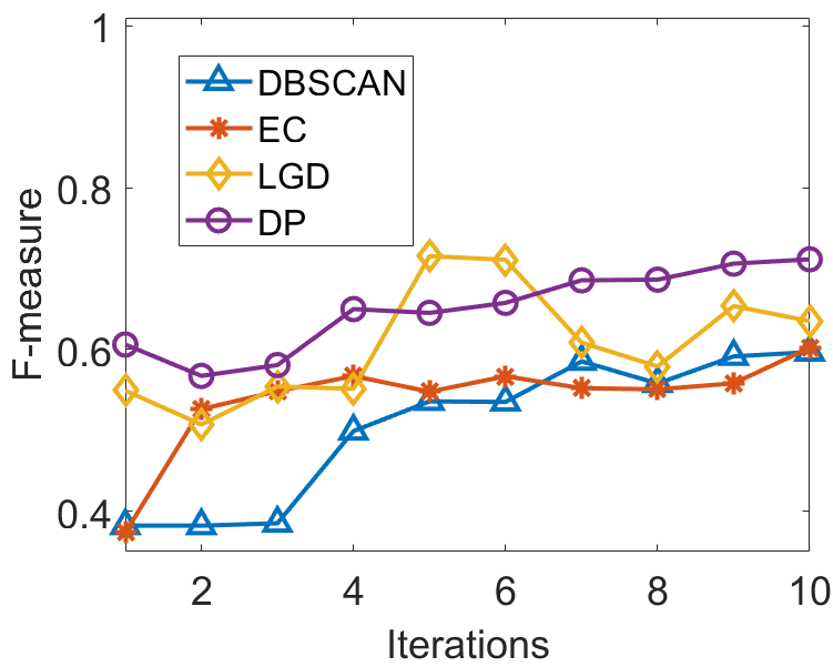
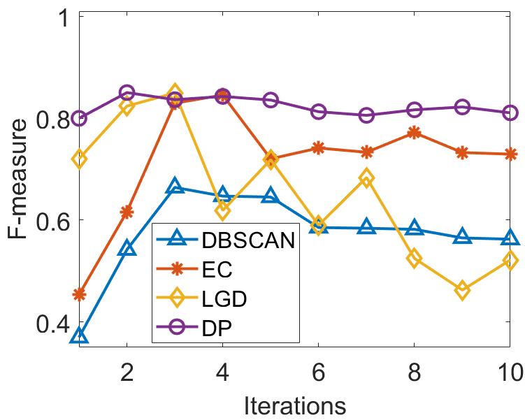
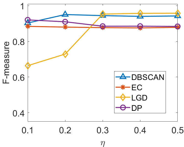
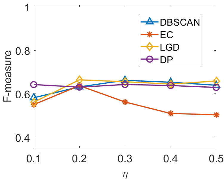
In this section, we select four datasets (4C, Haberman, Wilt and ForestType) in which CDF-TS significantly improves the performance of DBSCAN for the sensitivity analyses.

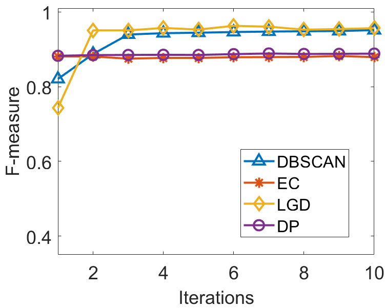
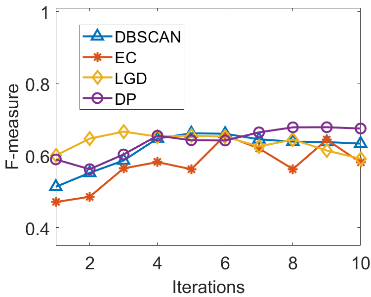
Figure 12 shows the best F-measure of the CDF-TS versions of four clustering algorithms with $\eta=0.3$ but different iterations from 1 to 10. The results show that only a few iterations allow most clustering algorithms to reach a good performance; while higher iterations may degrade the clustering performances of LGD and DBSCAN, as shown in Wilt and ForestType.

Figure 13 shows the best F-measure of the CDF-TS versions of four clustering algorithms with 5 iterations but different $\eta$. Most clustering algorithms can reach a good F-measure with $\eta=$ 0.2 or 0.3.

(a) 4C

(b) Haberman

(c) Wilt

(d) ForestType

Figure 12: The best F-measure of the CDF-TS versions of four clustering algorithms with $\eta=0.3$ but different iterations from 1 to 10 on four datasets.

(a) 4C

(b) Haberman

(c) Wilt

(d) ForestType

Figure 13: The best F-measure of the CDF-TS versions of four clustering algorithms with 5 iterations but different $\eta$ settings on four datasets.

References

- Aggarwal 2017 Charu C Aggarwal. Outlier Analysis. Springer International Publishing, Switzerland, 2nd edition, 2017. ISBN 978-3-319-47577-6.
- Aggarwal and Reddy 2014 Charu C Aggarwal and Chandan K Reddy. Data clustering. Algorithms and applications. Chapman&Hall/CRC Data mining and Knowledge Discovery series, Londra, 2014.
- Aksoy and Haralick 2001 Selim Aksoy and Robert M Haralick. Feature normalization and likelihood-based similarity measures for image retrieval. Pattern recognition letters, 22(5):563–582, 2001.
- Amini et al. 2016 Amineh Amini, Hadi Saboohi, Tutut Herawan, and Teh Ying Wah. Mudi-stream: A multi density clustering algorithm for evolving data stream. Journal of Network and Computer Applications, 59:370–385, 2016.
- Ankerst et al. 1999 Mihael Ankerst, Markus M. Breunig, Hans-Peter Kriegel, and Jörg Sander. OPTICS: Ordering points to identify the clustering structure. In Proceedings of the 1999 ACM SIGMOD International Conference on Management of Data, SIGMOD ’99, pages 49–60, New York, NY, USA, 1999. ACM. ISBN 1-58113-084-8.
- Bandaragoda et al. 2018 Tharindu R Bandaragoda, Kai Ming Ting, David Albrecht, Fei Tony Liu, Ye Zhu, and Jonathan R Wells. Isolation-based anomaly detection using nearest-neighbor ensembles. Computational Intelligence, 34(4):968–998, 2018.
- Blum and Langley 1997 Avrim L. Blum and Pat Langley. Selection of relevant features and examples in machine learning. Artificial Intelligence, 97(1):245 – 271, 1997. ISSN 0004-3702. Relevance.
- Borg et al. 2012 Ingwer Borg, Patrick JF Groenen, and Patrick Mair. Applied Multidimensional Scaling. Springer Science & Business Media, 2012.
- Breunig et al. 2000 Markus M. Breunig, Hans-Peter Kriegel, Raymond T. Ng, and Jörg Sander. LOF: Identifying density-based local outliers. SIGMOD Rec., 29(2):93–104, May 2000.
- Campello et al. 2013 Ricardo J. G. B. Campello, Davoud Moulavi, and Joerg Sander. Density-based clustering based on hierarchical density estimates. In Jian Pei, Vincent S. Tseng, Longbing Cao, Hiroshi Motoda, and Guandong Xu, editors, Advances in Knowledge Discovery and Data Mining, pages 160–172, Berlin, Heidelberg, 2013. Springer Berlin Heidelberg. ISBN 978-3-642-37456-2.
- Cassisi et al. 2013 Carmelo Cassisi, Alfredo Ferro, Rosalba Giugno, Giuseppe Pigola, and Alfredo Pulvirenti. Enhancing density-based clustering: Parameter reduction and outlier detection. Information Systems, 38(3):317–330, 2013.
- Chen et al. 2018 Bo Chen, Kai Ming Ting, Takashi Washio, and Ye Zhu. Local contrast as an effective means to robust clustering against varying densities. Machine Learning, pages 1–25, 2018.
- Demšar 2006 Janez Demšar. Statistical comparisons of classifiers over multiple data sets. Journal of Machine Learning Research, 7:1–30, 2006.
- Dua and Graff 2017 Dheeru Dua and Casey Graff. UCI machine learning repository, 2017. URL http://archive.ics.uci.edu/ml.
- Ertöz et al. 2003 Levent Ertöz, Michael Steinbach, and Vipin Kumar. Finding clusters of different sizes, shapes, and densities in noisy, high dimensional data. In Proceedings of the 2003 SIAM International Conference on Data Mining, pages 47–58. SIAM, 2003.
- Ester et al. 1996 Martin Ester, Hans-Peter Kriegel, Jörg S, and Xiaowei Xu. A density-based algorithm for discovering clusters in large spatial databases with noise. In Proceedings of the Second International Conference on Knowledge Discovery and Data Mining (KDD-96), pages 226–231. AAAI Press, 1996.
- Fahy and Yang 2019 Conor Fahy and Shengxiang Yang. Finding and tracking multi-density clusters in online dynamic data streams. IEEE Transactions on Big Data, 2019.
- Fawcett 2006 Tom Fawcett. An introduction to roc analysis. Pattern recognition letters, 27(8):861–874, 2006.
- Gramacki 2018 Artur Gramacki. Nonparametric kernel density estimation and its computational aspects. Springer, 2018.
- Hou et al. 2020 Jian Hou, Aihua Zhang, and Naiming Qi. Density peak clustering based on relative density relationship. Pattern Recognition, page 107554, 2020.
- Jolliffe 2011 Ian Jolliffe. Principal component analysis. In International encyclopedia of statistical science, pages 1094–1096. Springer, 2011.
- Kuhn 1955 Harold W Kuhn. The hungarian method for the assignment problem. Naval Research Logistics Quarterly, 2(1-2):83–97, 1955.
- Li et al. 2019 Ruijia Li, Xiaofei Yang, Xiaolong Qin, and William Zhu. Local gap density for clustering high-dimensional data with varying densities. Knowledge-Based Systems, 184:104905, 2019.
- Liu et al. 2008 Fei Tony Liu, Kai Ming Ting, and Zhi-Hua Zhou. Isolation forest. In 2008 Eighth IEEE International Conference on Data Mining, pages 413–422. IEEE, 2008.
- Liu et al. 2010 Fei Tony Liu, Kai Ming Ting, and Zhi-Hua Zhou. On detecting clustered anomalies using SCiForest. In Proceedings of the 2010 European Conference on Machine Learning and Knowledge Discovery in Databases: Part II, ECML PKDD’10, pages 274–290, Berlin, Heidelberg, 2010. Springer-Verlag. ISBN 3-642-15882-X, 978-3-642-15882-7.
- Lotfi et al. 2020 Abdulrahman Lotfi, Parham Moradi, and Hamid Beigy. Density peaks clustering based on density backbone and fuzzy neighborhood. Pattern Recognition, page 107449, 2020.
- Maaten and Hinton 2008 Laurens van der Maaten and Geoffrey Hinton. Visualizing data using t-sne. Journal of machine learning research, 9(Nov):2579–2605, 2008.
- Marin et al. 2019 Dmitrii Marin, Meng Tang, Ismail Ben Ayed, and Yuri Boykov. Kernel clustering: density biases and solutions. IEEE Transactions on Pattern Analysis and Machine Intelligence, 41(1):136–147, 2019.
- Ozertem et al. 2008 Umut Ozertem, Deniz Erdogmus, and Robert Jenssen. Mean shift spectral clustering. Pattern Recognition, 41(6):1924–1938, 2008.
- Pearson 1938 Egon Sharpe Pearson. The probability integral transformation for testing goodness of fit and combining independent tests of significance. Biometrika, 30(1/2):134–148, 1938.
- Qin et al. 2019 Xiaoyu Qin, Kai Ming Ting, Ye Zhu, and Vincent CS Lee. Nearest-neighbour-induced isolation similarity and its impact on density-based clustering. In Proceedings of the AAAI Conference on Artificial Intelligence, volume 33, pages 4755–4762, 2019.
- Ramaswamy et al. 2000 Sridhar Ramaswamy, Rajeev Rastogi, and Kyuseok Shim. Efficient algorithms for mining outliers from large data sets. In Proceedings of the 2000 ACM SIGMOD International Conference on Management of Data, SIGMOD ’00, pages 427–438, New York, NY, USA, 2000. ACM. ISBN 1-58113-217-4.
- Rijsbergen 1979 C. J. Van Rijsbergen. Information Retrieval. Butterworth-Heinemann, Newton, MA, USA, 2nd edition, 1979. ISBN 0408709294.
- Rodriguez and Laio 2014 Alex Rodriguez and Alessandro Laio. Clustering by fast search and find of density peaks. Science, 344(6191):1492–1496, 2014.
- Shi 2000 Jonathan Jingsheng Shi. Reducing prediction error by transforming input data for neural networks. Journal of computing in civil engineering, 14(2):109–116, 2000.
- Strehl and Ghosh 2002 Alexander Strehl and Joydeep Ghosh. Cluster ensembles—a knowledge reuse framework for combining multiple partitions. Journal of Machine Learning Research, 3(Dec):583–617, 2002.
- Szeliski 2010 Richard Szeliski. Computer vision: algorithms and applications. Springer Science & Business Media, 2010.
- Tan et al. 2020 Malong Tan, Shichao Zhang, and Lin Wu. Mutual knn based spectral clustering. Neural Computing and Applications, 32(11):6435–6442, 2020.
- Tenenbaum et al. 2000 Joshua B Tenenbaum, Vin De Silva, and John C Langford. A global geometric framework for nonlinear dimensionality reduction. science, 290(5500):2319–2323, 2000.
- Vinh et al. 2010 Nguyen Xuan Vinh, Julien Epps, and James Bailey. Information theoretic measures for clusterings comparison: Variants, properties, normalization and correction for chance. The Journal of Machine Learning Research, 11:2837–2854, 2010.
- Wang and Sun 2015 Fei Wang and Jimeng Sun. Survey on distance metric learning and dimensionality reduction in data mining. Data Mining and Knowledge Discovery, 29(2), 2015.
- Wang et al. 2011 Fei Wang, Bin Zhao, and Changshui Zhang. Unsupervised large margin discriminative projection. IEEE transactions on neural networks, 22(9):1446–1456, 2011.
- Wang et al. 2021 Shuliang Wang, Qi Li, Chuanfeng Zhao, Xingquan Zhu, Hanning Yuan, and Tianru Dai. Extreme clustering–a clustering method via density extreme points. Information Sciences, 542:24 – 39, 2021. ISSN 0020-0255.
- Zhu et al. 2016 Ye Zhu, Kai Ming Ting, and Mark J. Carman. Density-ratio based clustering for discovering clusters with varying densities. Pattern Recognition, 60:983 – 997, 2016. ISSN 0031-3203.
- Zhu et al. 2018 Ye Zhu, Kai Ming Ting, and Maia Angelova. A distance scaling method to improve density-based clustering. In Dinh Phung, Vincent S. Tseng, Geoffrey I. Webb, Bao Ho, Mohadeseh Ganji, and Lida Rashidi, editors, Advances in Knowledge Discovery and Data Mining, pages 389–400, Cham, 2018. Springer International Publishing. ISBN 978-3-319-93040-4.