CLEAR I: Ages and Metallicities of Quiescent Galaxies at $\mathbf{1.0<z<1.8}$ Derived from Deep
Hubble Space Telescope Grism Data

Abstract

We use deep Hubble Space Telescope spectroscopy to constrain the metallicities and (light-weighted) ages of massive ($\log M_{\ast}/M_{\odot}\gtrsim 10$) galaxies selected to have quiescent stellar populations at $1.0<z<1.8$. The data include 12–orbit depth coverage with the WFC3/G102 grism covering $\sim$ $8,000<\lambda<11,500$ Å  at a spectral resolution of $R\sim 210$ taken as part of the CANDELS Lyman-$\alpha$ Emission at Reionization (CLEAR) survey. At $1.0<z<1.8$, the spectra cover important stellar population features in the rest-frame optical. We simulate a suite of stellar population models at the grism resolution, fit these to the data for each galaxy, and derive posterior likelihood distributions for metallicity and age. We stack the posteriors for subgroups of galaxies in different redshift ranges that include different combinations of stellar absorption features. Our results give light-weighted ages of $t_{z\sim 1.1}=3.2\pm 0.7$ Gyr, $t_{z\sim 1.2}=2.2\pm 0.6$ Gyr, $t_{z\sim 1.3}=3.1\pm 0.6$ Gyr, and $t_{z\sim 1.6}=2.0\pm 0.6$ Gyr, for galaxies at $z\sim 1.1$, 1.2, 1.3, and 1.6. This implies that most of the massive quiescent galaxies at $1<z<1.8$ had formed $>68$% of their stellar mass by a redshift of $z>2$. The posteriors give metallicities of $Z_{z\sim 1.1}=1.16\pm 0.29$ $Z_{\odot}$, $Z_{z\sim 1.2}=1.05\pm 0.34$ $Z_{\odot}$, $Z_{z\sim 1.3}=1.00\pm 0.31$ $Z_{\odot}$, and $Z_{z\sim 1.6}=0.95\pm 0.39$ $Z_{\odot}$. This is evidence that massive galaxies had enriched rapidly to approximately Solar metallicities as early as $z\sim 3$.

1 Introduction

Astronomers have recently developed a general picture of the formation, chemical enrichment, and evolution of massive galaxies ($\log M_{\ast}/M_{\odot}\gtrsim 10-11$) from $z\gtrsim$ 3–4 to the present day. These galaxies formed their stellar populations early, reaching a peak star-formation rate (SFR) at $z>2$ (e.g., Labbé et al. 2005; Papovich et al. 2006; Madau & Dickinson 2014; Schreiber et al. 2016), and quenching as early as $z\sim 3-4$ (Spitler et al. 2014; Straatman et al. 2014; Glazebrook et al. 2017; Schreiber et al. 2018a, b). Massive galaxies continue to quench and remain in phases of quiescent evolution to lower redshift, where the fraction of quiescent galaxies with $\log M_{\ast}/M_{\odot}>10.5$ rises from $\sim$ 30% at $z\sim 2$ to $\approx$60% by $z=0.5$ (Muzzin et al. 2013; Tomczak et al. 2014; Kawinwanichakij et al. 2017). Because these massive galaxies formed their stars and quenched so early, they are testing grounds for physical processes associated with gas accretion, star-formation efficiency, feedback, metal production and retention (Oppenheimer et al. 2012; Somerville & Davé 2015; Torrey et al. 2017).

The next step is to understand in greater detail the galaxies’ star-formation and chemical enrichment histories. These effects are all encoded in the colors and spectral features of the galaxies’ stellar populations, which allows one to constrain the ages and metallicities using features that are sensitive to independent changes in these parameters. For example, line indexes (such as e.g., $D_{n}4000$, H$\delta$_A+H$\gamma_{A}$, H$\beta$, Mg$b$, [MgFe]^′, [Mg₂Fe]) have long been used to study these properties in galaxies, and to study their evolution with mass and redshift (e.g., Matteucci 1994; Trager et al. 2000; Thomas et al. 2005; Gallazzi et al. 2005, 2014; Renzini 2006; Choi et al. 2014; Wu et al. 2018).

Regarding the evolution of metals in galaxies, most studies have focused on the relation between the gas-phase metallicity (usually measured from emission line ratios in active galaxies) and galaxy stellar-mass, and their evolution with redshift (e.g., Tremonti et al. 2004; Erb et al. 2006; Zahid et al. 2014; Onodera et al. 2016; Sanders et al. 2017). It has been more difficult to measure evolution of metallicity of the stellar populations in galaxies. The spectral absorption and continuum features are sensitive to both $\alpha$-elements and Iron-peak elements (which dominate the opacity in stellar photospheres). Analyzing the spectra of quiescent galaxies at low-redshift ($z\lesssim 0.1$), many studies have found that massive galaxies have Solar (or super-Solar) metallicities and abundance ratios, with formation epochs at $z>2$ (e.g. Thomas et al. 2005, 2010; Gallazzi et al. 2005; Renzini 2006; Conroy et al. 2014). Gallazzi et al. (2014, hereafter Gal14) conducted one of the first studies at higher redshift ($z\sim 0.7$), and showed that the spectra of quiescent galaxies with $\log M_{\ast}/M_{\odot}>10.5$ are already consistent with high metallicity ($Z~{}\sim Z_{\odot}$), while star-forming galaxies have sub-Solar metallicities (and require additional enrichment from $z\sim 0.7$ to the present-day, see also Ferreras et al. 2018). The implication is that some fraction of the massive, quiescent galaxy population must have enriched to approximately Solar metallicities at even higher redshift, presumably at $z\gtrsim 2$.

To understand the evolution of massive quiescent galaxies therefore requires that we push spectroscopic studies to higher redshift, closer to the quenching epoch of these galaxies. The reason for this is that evolutionary changes in stellar populations occur on timescales $d\log t\propto dt/t$ (see e.g., Weisz et al. 2014). Therefore, galaxy properties change more rapidly at higher redshift (Tran et al. 2007; Eisenhardt et al. 2008; Blakeslee et al. 2009; Papovich et al. 2010), and more accurate (relative) measures of galaxy ages can be made by observing quiescent galaxies at $z>1$. The difficulty is that all the rest-frame optical spectral features used to measure both stellar population metallicities and ages shift above $\sim$1 µm for galaxies at $z>1$, where studies from ground-based telescopes are subject to higher backgrounds and a high density of telluric (night-sky) emission lines (see, Sullivan & Simcoe 2012). Several studies have now measured galaxy metallicities at high redshift with near-IR spectrographs on ground-based telescopes (e.g., Lonoce et al. 2015; Onodera et al. 2015; Kriek et al. 2016; Toft et al. 2017), but are often limited to one or a few objects or require stacking. An attractive alternative solution is to take advantage of space-based spectroscopy using, for example, the HST grisms, which have been used to study the properties of stellar populations in distant galaxies (e.g., Daddi et al. 2005; van Dokkum & Brammer 2010; van Dokkum et al. 2011; Whitaker et al. 2014; Momcheva et al. 2016; Fumagalli et al. 2016; Lee-Brown et al. 2017; Ferreras et al. 2018; Morishita et al. 2018).

Here, we use deep grism spectroscopy taken with HST spectroscopy with WFC3 using the G102 grism, covering wavelengths $\approx$8000 Å to 11,500 Å. We study the stellar populations of a sample of massive ($\log M/M_{\odot}\geq 10$) quiescent galaxies at $1<z<1.8$. At these redshifts, the G102 spectra cover crucial rest-frame optical absorption features at spectral resolution of $R\sim 210$, including the strength of the redshifted 4000 Å break, Balmer lines (H$\delta$, H$\gamma$,H$\beta$), Ca HK, and Mg$b$ absorption features) sensitive to stellar population ages and metallicities of galaxies down to $J\simeq 23-24$ AB mag. The G102 data also provide much improved measurements of the galaxy redshifts. We use a Bayesian method with a forward-modeling approach, whereby we simulate stellar population models of the two–dimensional (2D) WFC3/G102 spectra using the galaxies’ accurate morphologies at the appropriate roll-angle for HST combined with the G102 spectroscopic resolution.

One of the goals of this project is to determine the accuracy of stellar population properties measured with lower-resolution grism data. This has important implications for the next generation of space telescopes (JWST and WFIRST), and will allow the study of stellar populations of galaxies in much larger samples and at higher redshifts. As we push to higher redshifts, all important age- and metallicity-sensitive spectroscopic features shift into the IR. As we show here, even relatively low resolution ($R\sim 100-200$) spectroscopy can recover metallicity and age diagnostics of higher redshift galaxies (provided the spectra cover the age– and metallicity–sensitive features). This will have a wide range of application for future space missions.

The remainder of this paper is organized as follows: In Section 2 we describe the parent sample selection. In Section 3 we summarize the HST observations, data reduction, and spectral extraction methods. In Section 4 we describe the G102 spectral modeling procedure, including tests to demonstrate our ability to recover accurate stellar population parameters. We then discuss the model fits to the G102 data for the galaxies in our sample. In Section 5 we discuss the constraints on metallicities and (light-weighted) age for these galaxies, as well as implications for the formation, quenching and evolution of these galaxies. In Section 6 we present our conclusions and describe future work using this method. In the Appendices we show the model fits to the full galaxy sample, discuss our method to derive errors on model templates, discuss the Bayesian evidence in support of different stellar populations derived from the modeling, and we test our posterior stacking technique.

Throughout we use a cosmology with $\Omega_{M}=0.3$, $\Omega_{\Lambda}=0.7$, and $h$ = 0.7, where $H_{0}=100$ $h$ km s^-1 Mpc^-1 consistent with the recent constraints from Planck (Planck Collaboration et al. 2016) and the local distance scale of Riess et al. (2016). All magnitudes are in “absolute bolometric” (AB) units (Oke & Gunn 1983).

2 Parent Sample and Sample Selection

The HST WFC3 G102 grism wavelength coverage (8000 $<\lambda<$ 11500 Å) provides a wealth of information for distant galaxies as it probes the rest-frame UV and optical range for redshifts $z\sim 1$ (rest-frame coverage: 4000 $<\lambda<$ 5750 Å) to $z\sim 1.8$ (rest-frame coverage: 2850 $<\lambda<$ 4100 Å). These wavelengths cover many age– and metallicity–sensitive spectral features, including Ca HK, the 4000 Å/Balmer break, Balmer-series lines, several Lick indices, Mg$b$, and some Fe I lines (though not all features are covered at all redshifts by the G102 grism, as we will discuss below). With this in mind, we focused on a sample of quiescent galaxies selected to have low levels of star formation compared to their past averages. By modeling the spectra of such galaxies, we are able to constrain the galaxies’ star-formation histories (SFHs, when did they form their stars and when did they quench?), and enrichment histories (when did they form their metals?).

The CLEAR survey includes G102 observations within the CANDELS coverage of the GOODS-North deep (GND) and GOODS-S deep (GSD) fields (Grogin et al. 2011; Koekemoer et al. 2011). We selected galaxies from an augmented version of the photometric catalog from 3D-HST (Skelton et al. 2014; Momcheva et al. 2016) that includes photometry from $Y$–band imaging (using the WFC3 F098M and/or F105W imaging), which exists over the majority of the GND and GSD CANDELS fields (Koekemoer et al. 2011). More importantly, the WFC3 F098M and F105W filters provide imaging at comparable wavelengths covered by the WFC3 G102 grism, and is important for object extraction and identifying the locations of nearby objects that may cause spectral contamination.

The original 3D-HST data release did not include the F098M nor F105W data in the GOODS fields (because these have less uniform coverage, and are only available in two of the five CANDELS fields). Because we require them for our program, we have added them to the 3D-HST photometric catalog following the identical approach as Skelton et al. (2014). We first matched the PSFs of the F098M and F105W images to the detection image (using a weighted combination of the WFC3 F125W + F140W + F160W images). We then reran SExtractor (v2.8.6, Bertin & Arnouts 1996) in dual-image mode, using the detection image to photometer sources in the F098M and F105W images. We then inserted these fluxes into the existing 3D-HST catalogs along with rederived photometric redshifts and rest-frame $U-V$ and $V-J$ colors using EAZY (Brammer et al. 2008), and stellar masses from FAST (Kriek et al. 2009) (using a Chabrier (2003) IMF). For details of the procedures, see Skelton et al. (2014).

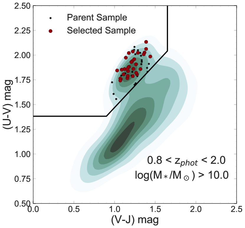
Figure 1: Distribution of rest-frame $V-J$ and $U-V$ colors of the galaxies in the GND and GSD galaxy samples. The green–shaded regions show the distribution of all galaxies in the parent catalog with $0.8\leq z_{\mathrm{phot}}\leq 2.0$, CLASS_STAR $<0.8$ from SExtractor, and $\log(M_{\ast}/M_{\odot})\geq 10.0$ (the two-dimensional shows all galaxies in this redshift and mass range, smoothed using an Epanechnikov (1969) kernel density estimation). The polygon delineates “quiescent” galaxies (upper left region) from “star-forming” (everywhere else) using the definition of Williams et al. (2009). Red points mark the sample of quiescent galaxies used here (these galaxies satisfy our selection requirements and fall in fields covered by the deep HST/WFC3 G102 spectroscopy). Unfilled points mark the sample of galaxies which were covered in the data and met most of the selection requirements, but were rejected from the final sample.

Table 1: Properties of the $1<z<1.8$ Quiescent Galaxy Sample

ID	$z_{phot}$	$J_{125}$ (Mag)	Log $(M_{\ast}/M_{\odot})$	SNR
(1)	(2)	(3)	(4)	(5)
GND23758	$0.94_{-0.04}^{+0.04}$	20.5	11.0	12.3
GND37955	$0.97_{-0.03}^{+0.03}$	21.3	10.8	7.3
GND16758	$0.99_{-0.03}^{+0.04}$	21.2	10.8	10.1
GSD43615	$1.04_{-0.04}^{+0.04}$	21.7	10.7	6.9
GSD42221	$1.04_{-0.04}^{+0.04}$	21.7	10.5	7.7
GSD39241	$1.04_{-0.04}^{+0.05}$	20.9	10.9	12.4
GSD45972	$1.05_{-0.02}^{+0.03}$	21.1	10.9	12.3
GSD44620	$1.08_{-0.03}^{+0.03}$	22.1	10.5	4.8
GSD39631	$1.08_{-0.03}^{+0.03}$	21.3	10.7	9.2
GSD39170	$1.08_{-0.02}^{+0.03}$	20.3	11.1	20.8
GND34694	$1.09_{-0.03}^{+0.04}$	21.0	10.9	9.9
GND23435	$1.09_{-0.06}^{+0.06}$	22.5	10.3	4.4
GSD47677	$1.10_{-0.04}^{+0.04}$	22.5	10.1	4.2
GSD39805	$1.16_{-0.03}^{+0.03}$	22.5	10.6	3.9
GSD38785	$1.18_{-0.03}^{+0.04}$	21.5	10.9	7.5
GND32566	$1.18_{-0.05}^{+0.05}$	21.7	10.6	6.6
GSD40476	$1.19_{-0.03}^{+0.03}$	21.9	10.6	8.6
GND21156	$1.20_{-0.04}^{+0.04}$	20.9	11.2	15.8
GND17070	$1.22_{-0.04}^{+0.04}$	21.2	10.9	5.3
GSD35774	$1.23_{-0.03}^{+0.03}$	21.0	10.9	10.0
GSD40597	$1.24_{-0.03}^{+0.03}$	20.9	11.0	16.3
GND37686	$1.27_{-0.04}^{+0.04}$	21.3	10.9	8.4
GSD46066	$1.32_{-0.03}^{+0.03}$	21.7	10.8	3.4
GSD40862	$1.33_{-0.04}^{+0.04}$	21.7	10.9	4.9
GSD39804	$1.36_{-0.03}^{+0.04}$	21.6	10.9	4.5
GND21427	$1.48_{-0.05}^{+0.05}$	22.0	10.7	2.5
GSD40623	$1.49_{-0.09}^{+0.11}$	22.3	10.8	4.7
GSD41520	$1.64_{-0.04}^{+0.04}$	22.2	10.9	3.4
GSD40223	$1.65_{-0.05}^{+0.05}$	22.7	10.7	2.3
GSD39012	$1.66_{-0.06}^{+0.06}$	22.6	11.1	1.8
GSD44042	$1.67_{-0.05}^{+0.05}$	21.8	11.0	4.0

Note. — (1) Galaxy ID number in the GND or GSD 3D-HST catalog. (2) photometric redshift from the 3D-HST catalog; (3) observed $J_{125}$ magnitude from the 3D-HST catalog; (4) stellar mass derived using FAST; (5) SNR per pixel measured at 8500-10500 Å in the stacked G102 spectrum.

It is our goal to select galaxies that are mostly devoid of star-formation, with a redshift that places the 4000 Å/Balmer break in the G102 grism wavelength coverage). We first selected a parent sample of galaxies to have photometric redshifts ($z_{phot}$) in the range $0.8<z_{\mathrm{phot}}<2.0$ and stellar mass $\log(M_{\ast}/\hbox{$M_{\odot}$})>10.0$. This $z_{phot}$ redshift range ensures that we select all galaxies that possibly place the 4000Å/Balmer break in the G102 wavelength coverage, when accounting for errors on the photometric redshifts. Our stellar-mass constraint ensures that the spectra have sufficient signal-to-noise for accurate modeling (see below). We filter stars from our parent sample, using objects that have stellarity values from the 3D-HST  catalog (defined by SExtractor) with CLASS_STAR $<0.8$. We remove any source with an X-ray detection (within a search radius of 0$\farcs$5) in the 2 Ms Chandra Deep Field-North Survey (Xue et al. 2016) and 7 Ms Chandra Deep Field-South Survey catalogs (Luo et al. 2017).

Based on the rest-frame $U-V$ and $V-J$ colors, we selected galaxies that are actively star-forming from those in quiescent phases of evolution (compared to star-forming/active galaxies, Wuyts et al. 2007; Williams et al. 2009; Whitaker et al. 2011). We selected a parent sample of quiescent galaxies from our augmented 3D-HST catalog using the definition in Williams et al. (2009),

$$(U-V)\ \geq\ 1.382\ \mathrm{mag},\$$

$$(V-J)\ \leq\ 1.65\ \mathrm{mag},\ \mathrm{and}\$$ (1)

$$(U-V)\ \geq\ 0.88\times(V-J)+0.59$$

Figure 1 shows the $U-V$ versus $V-J$ color distribution for the full galaxy catalog and for those galaxies in our parent sample. Galaxies in the quiescent UVJ region typically have specific SFRs (sSFRs) $<10^{-2}$ Gyr^-1 (Papovich et al. 2012), indicative of galaxies with lower current SFRs compared to their past averages (e.g., for a galaxy with a current stellar mass $10^{11}$ $M_{\odot}$ and sSFR=10^-2 $M_{\odot}$ yr^-1, the current SFR is $\Psi$=1 $M_{\odot}$ yr^-1, whereas the SFR averaged over the past Hubble time is $\langle\Psi\rangle$ $\sim$ 20 $M_{\odot}$ yr^-1). Galaxies with such low sSFR qualify as having “suppressed” SFRs (Kriek et al. 2006). Past studies of the evolution of these galaxies show they follow “passive” evolution of their mass-to-light ratios from redshifts as high as $z\sim 2$ (e.g., Fum16).

From the parent sample, we further require that all galaxies fall within the CLEAR HST/WFC3 G102 coverage (which includes 12 WFC3 pointings divided evenly between the GND and GSD fields, see Section 3). We then refit the galaxy redshifts using the G102 grism spectra themselves (as described in Section 5.1 below), and kept only those galaxies with $1.0<z_{grism}<1.8$ to ensure the G102 data cover the redshifted 4000 Å/Balmer break for all galaxies (this last step does exclude some galaxies with low SNR in the G102 data, typically $\langle SNR\rangle\lesssim 1.5$, see below). This yields our final sample of 31 galaxies. Table 1 shows the physical details of these galaxies.

For quiescent galaxies, the stellar mass limit of $\log M_{\ast}/\hbox{$M_{\odot}$}>10.0$ corresponds roughly to a magnitude limit of $J_{125}\leq 22.7$ mag at $z<1.8$. For such galaxies we measure a mean signal-to-noise ratio (SNR) in the G102 data of $\langle$SNR$\rangle$ $\gtrsim$3 per pixel, averaged over $\lambda$=0.85–1.05 µm (see Figure 2 and below). Most of the quiescent galaxies in our sample lie at stellar masses well above this limit, where the median mass is $\log(M_{\ast}/M_{\odot})=10.87$ with an interquartile range (spanning the 25th to 75th percentile) of $\log(M_{\ast}/M_{\odot})=10.67$ to 10.96.

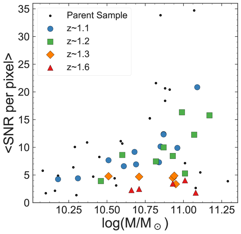
Figure 2: The average Signal-to-Noise ratio (SNR) measured in the HST/WFC3 G102 grism data for the galaxies in our samples as a function of galaxy stellar mass. For each galaxy, we measured the average SNR per pixel in the 1D spectrum over wavelengths $8500<\lambda<10500$ Å. For the majority of galaxies the average SNR is $>$3 per spectral pixel, where our tests show we are able to derive “good” physical constraints on the galaxy stellar population parameters.

3 HST WFC3/G102 Observations and Data Reduction

3.1 HST  Observing Strategy

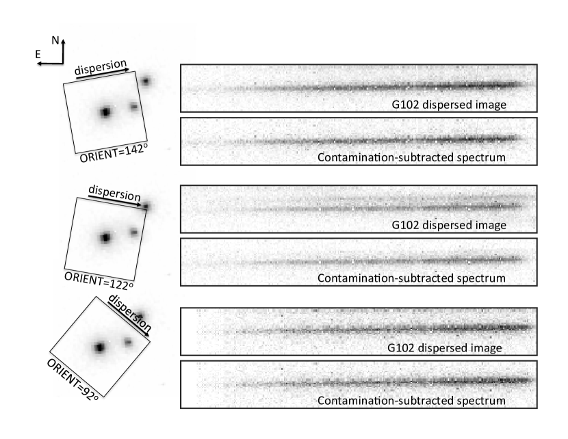
Figure 3: Example of HST imaging and spectroscopy for one object in our sample. The panels show the extracted F105W direct image and 2D G102 grism spectra for object GSD39170. The data are taken at three different PAs (ORIENT=142, 122, and 92 deg, as labeled). In each direct-imaging panel, the arrow shows the direction of the spectroscopic dispersion in the associated G102 image. Each panel contains a stack from four orbits at each PA, and shows the spectrum both before and after the subtraction from nearby sources (modeled during the the extraction process).

We use HST slitless spectroscopic data taken from the CANDELS Lyman-$\alpha$ Emission at Reionization (CLEAR; HST GO 14227, PI: Papovich). CLEAR covers 12 fields in the GND and GSD portions of CANDELS, with deep WFC3/G102 grism observations (12 orbits, when combined with some existing data). For unresolved sources the G102 dispersion is 24.5 Å/pixel^-1 (for the native WFC3 pixel scale, $\approx$0$\farcs$13/pixel), yielding a resolution of $R\sim 210$ at 1.0 µm.

The observations for CLEAR were taken over dates ranging from 2015 Nov 14 to 2017 Feb 19. Each pointing was observed for 10 or 12 orbits, with direct imaging in the WFC3 F105W ($Y_{105}$) paired with the G102 grism exposures. We followed the sub-pixel dither pattern used by 3D-HST (Brammer et al. 2012). The observations for each pointing were divided into 3 pointings of 4-orbits each (except in GND and the ERS field) separated by $\pm$10 degrees in roll angle to mitigate collisions of spectra from nearby objects and to avoid detector defects. In addition, we combined the CLEAR data with existing 2–orbit–depth data from other programs. The observations in the GND were only 10 orbits, and were combined with existing 2-orbit-depth data from the G102 from program GO 13420 (PI: Barro). The observations in the ERS were combined with existing 2-orbit-depth G102 data from the WFC3 ERS program (PI: O’Connell; see Windhorst et al. 2011; Straughn et al. 2011).

During the scheduling of the CLEAR observations, care was taken to protect the G102 grism data from a known time-variable background. This background is due to He I emission from the Earth’s atmosphere at 10830 Å, which contributes to the background in the $Y$–band (and G102 grism) when HST observes at low limb angles (see Brammer et al. 2014; Tilvi et al. 2016; Lotz et al. 2017). Following the strategy of the Hubble Frontier Fields (Lotz et al. 2017), we monitored the predicted observational ephemeris of each CLEAR observation. We then structured the observing sequence to place the direct imaging (F105W) observation at the end (or start) of the orbit when the He I emission was expected to have the largest impact, and to place the grism (G102) observation at the start (or end) of the orbit to take advantage of the lower background levels.

3.2 HST Spectroscopic Data Reduction

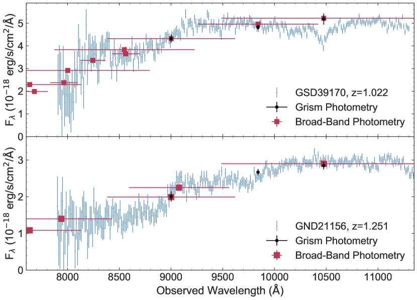
Figure 4: Example comparison of the flux-calibration of our 12-orbit depth 1D G102 grism spectra (blue) to the broad-band photometry (red) from our 3D-HST catalog (that includes available $z_{850}$, $Y_{105}$, or $Y_{098}$ data) for two objects in our sample. Black points show the synthesized $z_{850}$, $Y_{105}$, and $Y_{098}$ measurements from the grism data. The horizontal bars on the photometric points show the FWHM of the broad-band filter transmission curves. Vertical error bars show the 1 sigma errors. Filters included in the top panel are the F775W, IA767, IA797, F814W, IA827, I, IA856, $z_{850}$, $Y_{098}$, and $Y_{105}$ bandpasses. The filters included in the bottom panel are the F775W, I, $z_{850}$, Z, and $Y_{105}$ bandpasses.

The data reduction of the G102 spectra follow the procedures from the 3D-HST pipeline^, (Brammer et al. 2012; Momcheva et al. 2016) and custom scripts. This includes interlacing of the data to reduce pixel-to-pixel correlations (c.f., drizzling). Following the calwf3 processing, we inspect the images for artifacts (satellite trails) and any regions of elevated background. Satellites typically affect a single WFC3 grism read, and in those instances, we remove the read (or reads) containing the satellite trail. If they persisted we masked them. We then rejected cosmic rays by using AstroDrizzle.

To calibrate the G102 images we first divided them by the WFC3/F105W imaging flat field (see Brammer et al. 2012) and then subtracted the background following the methods in Brammer et al. (2014). We then subtracted the masked column average in each image to create the final background–subtracted images and to remove low-level residuals not accounted for in the backgrounds. Lastly, we combined the exposures taken at the same ORIENT using the interlacing discussed in Momcheva et al. (2016). This provided stacked grism images containing between two and four orbits of data.

From these stacked grism images we extracted 2D and 1D spectra for individual objects in our sample defined in Section 2 using the procedures in (Momcheva et al. 2016). We required a reference direct image to provide the positions and morphologies of each object for spectroscopic extraction. As described by Momcheva et al. (2016), the pipeline uses the direct image to identify and model the expected location of spectral traces associated with contaminating sources, using the positions and redshifts of sources in the input catalog (see Section 2).

We used the WFC3 F105W mosaics for all extractions, and for the modeling and subtraction of contamination from nearby sources (we found that using the F105W provided the best contamination modeling and subtraction compared to other WFC3 bands, likely because the F105W matches the wavelength coverage of the G102 data).

Prior to stacking spectra for each object, we visually inspected the data to ensure they were not affected by severe contamination or by other cosmetic issues. In most cases, the pipeline removed most of the contamination from nearby sources. In rare cases we identified residual contamination present in one of the stacks (in all but one case for our sample this affected only one ORIENT). In this case we either discarded the contaminated stack, or if the contamination was minor, we masked affected pixels before stacking the extracted spectra.

Figure 3 shows the CLEAR data for one of the galaxies in our sample (GSD 39170 with a redshift derived from the grism spectrum of $z_{grism}=1.02$, see below), which shows the direct imaging and grism data extracted from the 4-orbit depth stacks at each of the three different roll angles (ORIENTs). This target highlights the contamination subtraction capabilities of the CLEAR pipeline, as a contaminating source lies near our target. In one orient its spectrum falls near the target, and in another it lies directly over our spectrum. Using multiple orients we can characterize the contaminating source spectrum, and subtract it from the raw data.

3.3 Tests of the HST G102 Grism Flux Calibration

Our study requires that the relative flux calibration of the HST WFC3/G102 grism data be accurate as we use the continuum in our analysis of the galaxy stellar populations. In general, the absolute flux calibration of HST is very stable with average temporal variations constrained to be less than 1% (Lee et al. 2014), and allows us to use the continuum for this purpose. This is a significant advantage of space-based slitless spectroscopy compared to slit-fed spectroscopy from the ground, which suffers from systematics associated with terrestrial, astronomical, and instrumental backgrounds (Sullivan & Simcoe 2012), and partly explains why slitless spectroscopy with HST is superior in some aspects compared to ground-based 10 m-class telescopes (Momcheva et al. 2016; Tilvi et al. 2016), even though the current HST IR instruments operate at lower spectral resolution.

Figure 5: Difference between the $\hbox{$z_{850}$}-\hbox{$Y_{098}$}$ color derived from broad-band photometry and the color in those bands synthesized from the G102 spectra, plotted as a function of the G102 SNR measured at 8500-10500 Å. Here we can see the residuals are consistent with zero.

We tested the flux calibration of the extracted grism data for objects in our sample by comparing the spectra with the broad-band flux measurements from HST broad-band imaging. We synthesized photometry from the grism spectra by integrating them with the HST ACS F850LP and WFC3 F098M filters ($z_{850}$ and $Y_{098}$), as these cover wavelengths also covered by the G102 grism. Figure 4 shows a comparison of the (flux-calibrated) extracted G102 spectra for two objects in our sample (GSD 39170 and GND 21156) to their broad-band photometry from our augmented 3D-HST catalog (see Section 2). The overall agreement between the broad–band and synthesized photometry is better than 3%.

Next, we investigated the accuracy of the relative flux as a function of wavelength (i.e., the accuracy of the “color” of the spectra as these would impact our ability to measure stellar population parameters, such as the ages and metallicity). The G102 grism covers wavelengths also covered entirely by the ACS F850LP and WFC3 F098M filters, and we therefore focus only on the subset of objects in the GSD (ERS) that have coverage in both band-passes. Figure 5 compares the $\hbox{$z_{850}$}-\hbox{$Y_{098}$}$ color synthesized from the G102 data to the color measured directly by these bands in our photometric catalog, plotted as a function of SNR in the G102 grism spectrum measured at 8500-10500Å. Taking all objects, the median color difference is $\Delta(\hbox{$z_{850}$}-\hbox{$Y_{098}$})=0.05$ mag, this is consistent with a measurement of 0.0 mag as our measured errors are larger than the offset. Therefore we conclude that the grism flux calibration is accurate (compared to the broad-band colors), and we consider any systematic uncertainty in flux calibration to be negligible in our analysis.

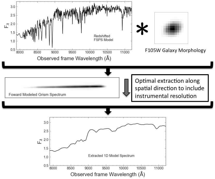
Figure 6: Flow chart of the forward modeling process for the G102 spectra. Top row shows the input, observed frame spectrum with the native resolution of the stellar population synthesis model (in this case FSPS; top left panel). This is then convolved with the $Y$–band (F105W or F098M) imaging (second right panel) and G102 grism resolution to produce an accurate model of the 2D G102 spectrum for this galaxy for this stellar population model (illustrated in the middle row). We then optimally extract a 1D spectrum for this model, which now includes an accurate G102 spectroscopic resolution (that includes the morphological broadening appropriate for each galaxy). For each galaxy we build a suite of these models over a range of stellar population parameters, which we then fit to the observed spectra for each galaxy.

4 Methods and Tests of Model Fitting

Our primary goal is to constrain the ages and metallicities of the quiescent galaxies in our sample. Here, we describe our method to model the spectra, to fit them to the data, and to extract posteriors of the stellar population parameters.

4.1 Forward Modeling of HST Grism Data Using Stellar Population Models

We use composite stellar population models in order to investigate the SFHs, ages, and metallicities of the quiescent galaxies at $1.0<z_{grism}<1.8$ in our sample. To generate model spectra, we tested two sets of models: the Flexible Stellar Population Synthesis (FSPS) models (Conroy et al. 2009; Conroy & Gunn 2010); and the set of models from Bruzual & Charlot (2003, BC03). The FSPS models use isochrones from the Padova stellar evolution tracks, with the MiLeS empirical stellar library for wavelengths $3500<\lambda/\hbox{\AA}<7500$ (and BaSeL theoretical spectra elsewhere). The BC03 models use the Padova tracks and isochrones combined with the STELIB empirical stellar library for wavelengths $3200<\lambda/\hbox{\AA}<9500$ and BaSeL spectra elsewhere. For both the BC03 and FSPS models we assume a Salpeter (1955) IMF (although this has minimal impact on the age or metallicity constraints we infer).

While we consider both BC03 and FSPS for our model fitting. In Appendix C, we find Bayesian evidence against the BC03 models in favor of the FSPS models. Fum16 obtain similar results, where they show that FSPS models provide better agreement (lower $\chi^{2}$ values) for fits to stacked quiescent galaxy spectra of similar resolution and rest-frame wavelength. We therefore report results from the FSPS for the remainder of this work in light of the Bayesian evidence against the BC03 models.

We generated a large range of spectra from the FSPS models, spanning a range in age ($t=0.5-6.0$ Gyr, in steps of 0.1 Gyr), metallicity ($Z=0.1-1.6$ $Z_{\odot}$ in steps of 0.05 $Z_{\odot}$), and SFH ($\tau=0.0-3.0$ Gyr in steps of 0.1 Gyr). Regarding the metallicity, as we fit to the full spectra, our measurements of the metallicities are affected both by the individual elements in the spectral absorption features and those that affect the stellar opacities that make up the continua. Since the latter are dominated primarily by Iron peak elements (Conroy et al. 2014), we expect that the “metallicity” ($Z$) here is a proxy for [Fe/H]. Nevertheless, there is evidence for higher abundances of [$\alpha$/Fe] in massive galaxies at low redshift (see, e.g., Matteucci 1994; Thomas et al. 2005; Choi et al. 2014; Conroy et al. 2014, and references therein) and some evidence for this in galaxies at high redshift (Kriek et al. 2016; Steidel et al. 2016). Future modeling of the abundance of individual elements would provide more detailed insight into chemical enrichment histories of galaxies.

We assume "delayed $\tau$" SFHs that increase linearly with time followed by an exponential decay characterized by an e-folding timescale $\tau$, such that the star-formation rate (SFR, $\Psi(t)$) at a given age, $t$, is parameterized by $\Psi(t)\propto t\times\exp(-t/\tau)$. These best represent the average SFHs of quiescent galaxies at early and late times (e.g., Papovich et al. 2011; Simha et al. 2014; Pacifici et al. 2016; Iyer & Gawiser 2017). In our analysis we marginalize over $\tau$ as a nuisance parameter.

For the remainder of this work, we interpret the age using the “light–weighted” ages, $\langle t\rangle_{L}$, which have been averaged over the past SFH weighted by the luminosity of the stellar population. This is because $\langle t\rangle_{L}$ best corresponds to the age of the stellar populations that dominate the galaxy light. This is more robustly quantifiable than the SFH itself (see e.g., Papovich et al. 2001; Salmon et al. 2015), and best represents the age of the stars that dominate the observed spectrum (see also Fum16). We derive the light-weighted ages using the SFHs and (instantaneous) ages as

$$\langle t(t^{\ast},\tau)\rangle_{L}=\frac{\int_{0}^{t^{*}}\Psi(t,\tau)\ L(t^{*}-t,\tau)\ (t^{*}-t)\ dt}{\int_{0}^{t^{*}}\Psi(t,\tau)\ L(t^{*}-t,\tau)\ dt}$$ (2)

where $t^{\ast}$ is the instantaneous age of the model. The quantity $L(t^{*}-t,\tau)$ is the luminosity at an age of $t^{*}-t$, for a given SFH, $\Psi(t,\tau)$, measured in a given filter band (we use the SDSS $g$ band in the rest frame).

To include the effects of dust, we attenuate the model spectra by the value $A(V)$ using the Calzetti et al. (2000) dust law (to be consistent with the dust measurements from 3D-HST Skelton et al. 2014).

$$F(\lambda)_{\mathrm{observed}}=F(\lambda)_{\mathrm{unattenuated}}\times 10^{-0.4\ k(\lambda)\ A(V)/R(V)}$$ (3)

where $k(\lambda)$ is the starburst reddening curve, and $R(V)$ is the total–to–selected attenuation in the $V$-band, with $R(V)=4.05$.

We then simulated the 2D and 1D grism spectra from using the stellar population models with the software package Grizli (the grism redshift and line analysis software), developed by CLEAR team member (G. Brammer). Grizli uses as input the stellar population model spectrum, the galaxy redshift, and the galaxy image to correctly model the 2D grism data. For this latter step, we use imaging from F105W (or F098M) from CANDELS. Using the correct morphology is highly important, as the galaxy morphology effectively “smooths” the resolution of the (slitless) grism spectrum (referred to as “morphological broadening”, van Dokkum et al. 2011), which is caused by the image of the galaxy dispersed over the range of wavelengths covered by the grism. The broadening of features is therefore correlated to the morphology of the galaxy (and at the resolution of our data this is the dominant effect; we can neglect the contribution from dynamical motions within the galaxy). The correlation with morphology means the spectral resolution decreases with increasing galaxy size (where narrow lines can be lost or smoothed over). More compact galaxies, due to their smaller size, will produce the least morphologically broadened spectra (i.e., they will have higher spectral resolution). This modeling process of the data is illustrated in Figure 6.

We further adopt an additional “uncertainty” to account for systematic errors, which could either arise from incompleteness or inaccuracies in the stellar population models, or from systematic errors in the data (see e.g., discussion in Papovich et al. 2001; Brammer et al. 2008). To counter this “model error” we add an additional systematic error term (a template error function) following Brammer et al. (2008) (detailed in Appendix B) .

4.2 Fitting Grism Models to Grism Data

In what follows we describe fitting the 1D spectral models derived from Grizli and the stellar populations to the 1D G102 data for each galaxy. Because we are considering only a small number of parameters at present, we generate models over a grid of parameter values. We derive a $\chi^{2}$ goodness-of-fit measurement for each combination of model for the G102 data, and we then calculate a likelihood distribution using the following,

$$P(D|\Theta)\propto\exp(-\chi^{2}/2)$$ (4)

where $D$ is the data and $\Theta$ is the set of parameters we consider. We derive the joint probability density function using Bayes’ theorem

$$P(\Theta|D)\propto{P(D|\Theta)P(\Theta)}$$ (5)

where $P(\Theta)$ represents prior information. Here we assume “flat” priors over the parameter range (see discussion in Salmon et al. 2015); for metallicity, (light-weighted) age, SFH, and redshift. For the dust attenuation, we use a prior derived by fitting a skewed Gaussian to the distribution of $A(V)$ values derived from broad-band photometry from 3D-HST for galaxies in our redshift and mass range. We then marginalize to get posteriors on individual parameters. For example, given $\Theta$ = ($X$, $Y$, $Z$), we would derive the posterior on parameter $X$ as,

$$P(X)=\int_{Y}\int_{Z}\ P(X,Y,Z|D)\ dZ\ dY$$ (6)

In the sections that follow, we test the ability of our method to recover model parameters using simulated data. We first test the results for model stellar populations in different redshift ranges (Section  4.2.1). Next, we test the accuracy of recovered stellar population parameters for models fit to simulated data with and without the spectral continua (Section 4.2.2). As a result of these tests we concluded a best practice to (1) sub-divide galaxies by redshift so that the G102 spectra cover different spectral features which allows us to study systematics resulting from differences in rest-frame wavelength coverage, and (2) fit the full spectrum including the continua as this provides the most accurate constraints on the stellar population parameters. Following these tests we apply these methods to (re-)measure galaxy redshifts from the G102 grism data (Section 5.1). We then fit the grism data to derive stellar population parameters for the galaxies in our sample. (Section 5.2).

4.2.1 Tests using Simulated Data in Different Redshift Ranges

We tested our ability to measure meaningful constraints on model parameters of galaxies at different redshifts. We selected (direct) images and redshifts from four real galaxies in our sample, and input models with 6 different combinations of parameter values spaced throughout a plausible range of values; $t=1.9$ to $4.5$ Gyr, $Z=$ 0.42 to 1.32 $Z_{\odot}$, and a delayed SFH with $\tau=0.5$ Gyr. In all cases, we simulated model spectra, as illustrated in Figure 6. For the simulated “data” we added real noise measured from extracted the G102 spectral data.

We then fit the simulated model data using the method described in Equations 4–6, fixing redshift to the true value and setting A($V$)$=0$. We repeated these simulations 1000 times (for each set of “truth” parameters) to generate likelihoods for the accuracy of the recovered parameters. One limitation of this simulation is that model spectra exactly match the (simulated) “data”, but this allows us to determine the limitations of the fitting procedure in the idealized case before applying it to real data. We then derived posteriors on the model parameters.

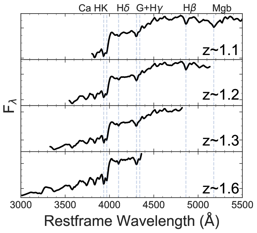
Figure 7: Comparison of redshift subgroups. Each panel shows the portion of the rest-frame spectrum covered by the G102 in each redshift subgroup. Important age– and metallicity–sensitive spectral features are labeled.

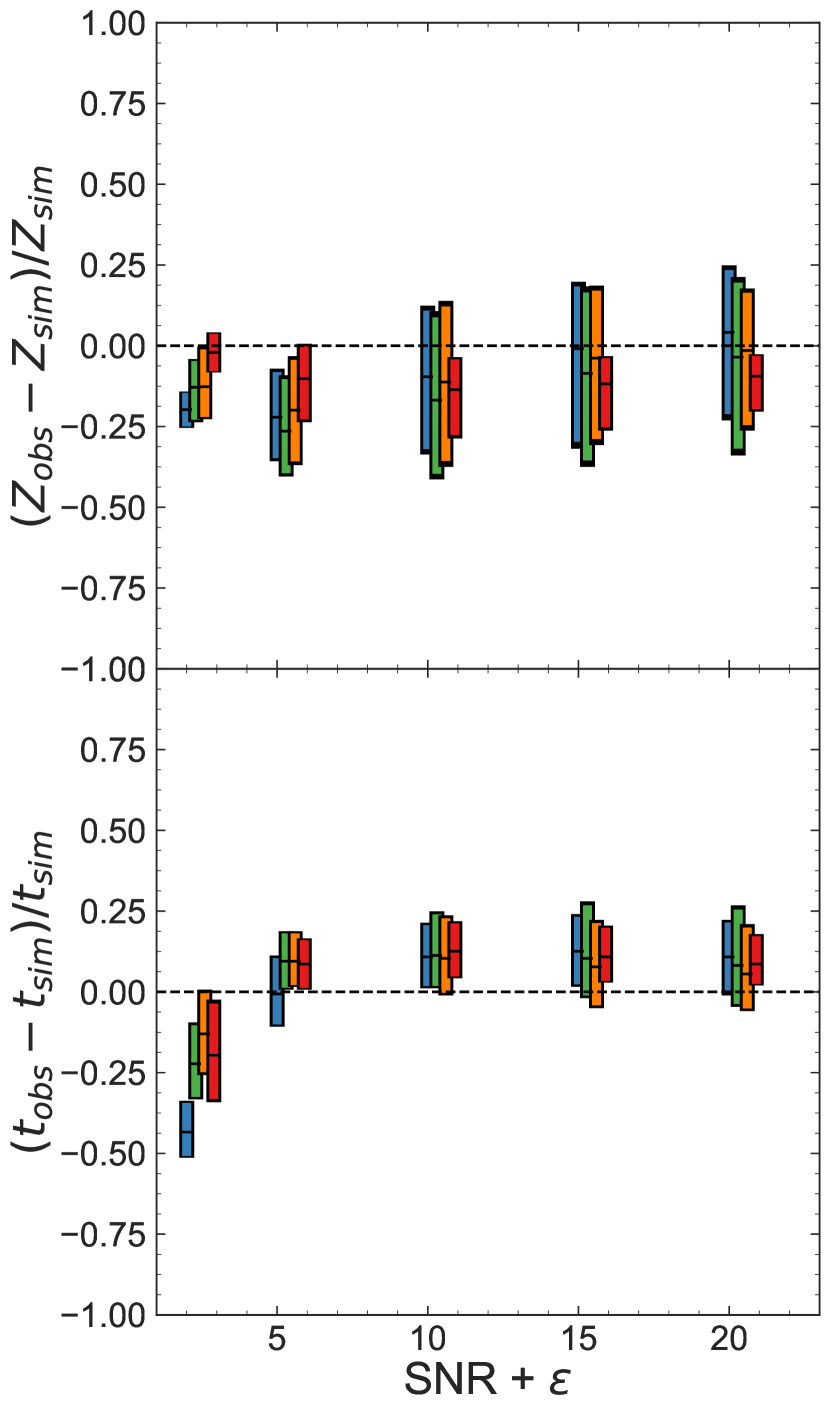
Figure 8: Illustration of the distribution of fits on stellar population parameters derived from fits to simulated data. This was done for each redshift subgroup as a function of SNR (shown with a slight offset ($\epsilon$) for readability). Fits shown here are in relation to simulated spectra with “true” values $t=$2.5 Gyr and $Z=$1 $Z_{\odot}$ . Because the G102 spectrum probes different portions of the rest-frame spectrum, the accuracy of the derived parameters changes as the important features shift across the grism coverage.

Inspecting our results, we identified four natural redshift ranges which probe different rest-frame spectroscopic features, and therefore have slightly different systematics in the results from the fitting. These redshift ranges have medians of approximately $z=1.1$, 1.2, 1.3, and 1.6, and correspond to where the different age– and metallicity–sensitive spectral features shift in and out of the grism wavelength coverage, as illustrated in Figure 7. At all redshifts ($1.0<z_{grism}<1.8$) the G102 spectra contain the 4000 Å/Balmer break, which provides constraining power on the ages and metallicities of the stellar populations.

Figure 8 shows the measured distributions on (light-weighted) age ($t$) and metallicity ($Z$) for simulated models, for one combination of “true” (light-weighted) age $t=$2.5 Gyr and metallicity $Z=$1 $Z_{\odot}$, in each of the four redshift bins (we obtain similar results for other combinations of age and metallicity, but show these as they are close to the values we derive for the real data for the galaxies in our sample).

In what follows we qualitatively describe the fits in each subgroup for one set of parameters. This set was chosen as it represents a region of the parameter space we expect to be well populated. We quote values for fits of spectra with SNR = 10 (as an example of how well “good” spectra can constrain parameters), though we find that we are able to recover the parameters accurately down to SNR $\sim$ 3.

For the first redshift subgroup, z $\sim$ 1.1 ($1.00<z_{grism}<1.16$), the G102 data cover wavelengths that probe features out through Mg$b$. Unlike the Balmer lines, which are mostly age dependent, including the Mg$b$ feature provides improved constraints on metallicity. The age constraints are also reliable, but suffer from the lack of spectral coverage the rest-frame $U$-band data.

The second redshift subgroup, z $\sim$ 1.2 ($1.16<z_{grism}<1.30$), includes features out through H$\beta$. The lack of Mg$b$ could make constraining metallicity more difficult, but with a better defined 4000 Å break and coverage of the rest-frame $U$ band these data probe the shape of the rest-frame $U$–$B$ continuum and yields relatively accurate constraints on the age and metallicity.

The third redshift subgroup, z $\sim$ 1.3 ($1.30<z_{grism}<1.45$), contains galaxy spectra that lack coverage of Mg$b$ and H$\beta$, but still contain the G+H$\gamma$ features. The constraints on the age are aided due to stronger presence of the rest-frame $U$–$B$ continuum.

The fourth subgroup is our highest redshift group, z $\sim$ 1.6 ($1.45<z_{grism}<1.70$). The most prominent features of the z $\sim$ 1.6 group are the 4000 Å break and the large amount of $U$–$B$ continuum. This group differs from the z $\sim$ 1.3 group by having the $H_{\gamma}$ feature in a noisy region of the spectra.

For the all groups, we are able to recover the metallicities and light-weighted ages with typical uncertainties of $\sigma(Z)$$\approx$0.30 Z_⊙ and $\sigma(t)$$\approx$0.3 Gyr ($\sigma(t)$$\approx$0.2 Gyr for z $\sim$ 1.6) respectively. The tighter constraint seen in the z $\sim$ 1.6 age measurement is an artifact of the definition of SNR. We use the SNR per pixel, averaged over 8500–11,500 Å. For $z\sim 1.6$, this observed wavelength range mostly covers the $U$ band, and the portion around (and above) the rest-frame 4000 Å/Balmer break has much higher S/N.

When taking all redshift subgroups, and parameters into account, Figure 8 indicates there may be a slight bias in light-weighted age and metallicity on the order of $\approx+10\%$ and $\approx-10\%$, respectively (for SNR $>$ 5). However, these biases are small relative to the constraints we derive on these parameters for each galaxy. We therefore make no attempt to correct these.

Figure 9: Comparison of parameter distributions from fitting with and without the continuum. The top panel shows the posteriors on the metallicity distributions. The bottom panel shows the light-weighted age distributions.

4.2.2 Tests Using Simulated Data with and without Continua

We performed an additional test to determine the importance of fitting to the galaxy spectra including the continuum and fitting with the continuum divided out. Although we show in Section 3.1 that the flux calibration is not a significant source of error, past studies frequently remove the continuum, allowing for fits directly to the stellar population features, and mitigating against uncertainties in flux calibration (Conroy & Gunn 2010, Fum16). However, there is information in the continuum as it is the superposition of the photospheres of the composite stellar populations, whose characteristics depend strongly on age, metallicity and SFH. As we have determined that the HST flux calibration is both accurate and stable, including the continuum provides important information for the model fits.

For our test, we removed the continua (on the models and simulated “data”) by dividing the spectra with a third order polynomial fit, masking out regions with possible emission or absorption features except for the 4000 Å break. We then fit the models to the data, derived likelihoods, and marginalized over parameters to derive posteriors.

Figure 9 compares the recovered parameters derived by fitting simulated spectra with and without the continuum. The abscissa in both the top and bottom panels show the difference between the true value and the derived median value. We smooth the distribution of points with a kernel density estimator to derive the likelihood. While we recover, on average, the true value for both cases, using the continuum provides a tighter and more symmetric distribution, with improved results. Formally, using the continuum, we derive median and 68% confidence intervals for the offset in metallicity and light-weighted age as $\Delta Z_{c}=-0.013_{-0.22}^{+0.19}$ $Z_{\odot}$ and $\Delta t_{c}=-0.26_{-0.46}^{+0.59}$ Gyr. Using fits to data where the continuum has been divided out, we derive $\Delta Z_{nc}=-0.013_{-0.27}^{+0.32}$ $Z_{\odot}$ and $\Delta t_{nc}=-0.08_{-0.86}^{+0.71}$ Gyr. For the case that includes fits to the full spectra (i.e., including the continua and all absorption features), the offsets and uncertainties are smaller (and the posterior is more symmetric). We therefore fit to the full spectra in our analysis of the galaxies in our sample=.

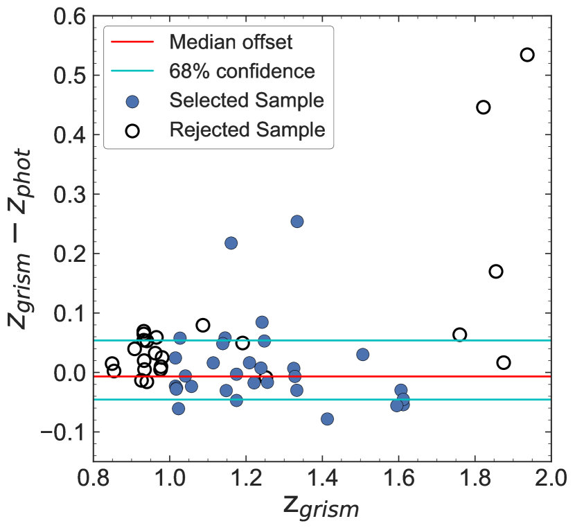
Figure 10: Comparison of our photometric redshifts derived from the deep CLEAR G102 spectra ($z_{grism}$) to those derived from broad–band photometry from 3D-HST ($z_{phot}$). The median offset between the two redshifts ($\Delta z\sim$ 0.01) is marked by a red line and the 68% scatter intervals ($-0.07<\Delta z<0.04$) are bounded by cyan lines. Empty circles mark the rejected sample; this includes the sample of galaxies rejected after fitting $z_{grism}$.

5 Results

5.1 Measuring Redshifts from the Grism G102 Data

It is important to have accurate redshifts when modeling the galaxy stellar populations. We therefore re-derived galaxy redshifts, $z_{grism}$, by fitting the model grism spectrum to the data, using an iterative method. We firstly fit $z_{grism}$ over a coarse grid of model parameters to estimate its value. We secondly fit $z_{grism}$ over the full set of parameters but limiting the range of redshifts. These two steps saved computation time by a factor of $\approx$25.

For the first $z_{grism}$ iteration, we generated models with fixed $\tau$ = 100 Myr over a coarser grid of metallicities and ages, with a very fine grid of redshift ($\Delta z=0.001$) over a range of $0.8<z<2.0$. For the galaxies in our sample, the choice of $\tau$ does not affect the measurement of $z_{grism}$ for $\tau<500$ My for the quiescent galaxies in our sample. We fit using the set of parameters $\Theta=(Z,t,z_{grism})$, and then marginalize to obtain a posterior on $z_{grism}$,

$$P(z_{grism})=\int_{Z}\int_{t}P(Z,t,z_{grism})\ dt\ dZ$$ (7)

From the $P(z)$ we derive median values and a 68%-tile range on $z_{grism}$ for each galaxy. These median values are used in our full model fitting (below) to set the redshift range used (where we fit over a range $z_{median}\pm dz$ with $dz=0.02$ (which spans the peak and majority of the probability mass in redshift space for galaxies in our sample). Table 2 reports the median and 68% confidence interval on $z_{grism}$ from these fits. The grism-derived redshifts have typical uncertainties $\sigma_{z}\lesssim 0.004$, and are significantly improved compared to the broad-band-derived photometric redshifts with $\sigma_{z}\approx 0.02-0.11$ (see Table 1 and Figure 10). Similar results are seen in Momcheva et al. (2016)

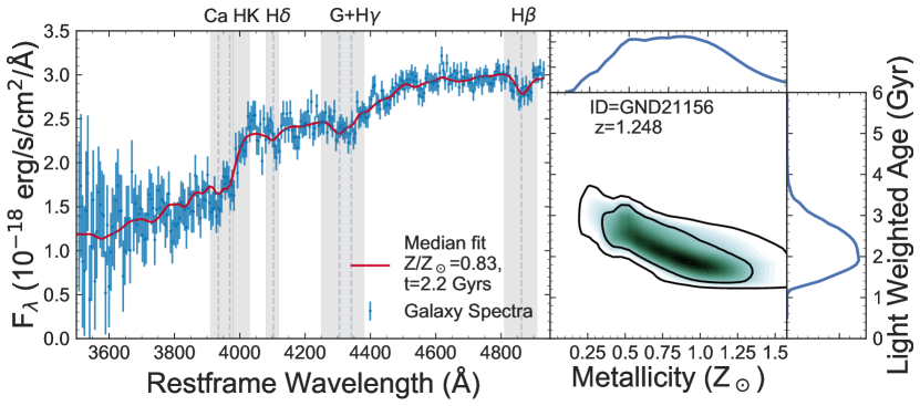
Figure 11: Left: The 1D G102 grism 12-orbit data for the galaxy GND21156 at $z=1.251$ as a function of rest-frame wavelength. The shaded regions show the locations of prominent spectral features. The red solid line shows a model with parameters given by the median metallicity ($Z$) and light-weight age ($t$) derived from the posteriors derived on each parameter. Right:The posteriors on the stellar population parameters of metallicity and light-weighted age for the galaxy in the left panel. The main panel shows the joint likelihood (with the 68$\%$ and 95$\%$ confidence intervals outlined in black) derived on both parameters jointly using Equation 6. The sub-panels to the right and above the main panel show the individual posteriors on light-weighted age and metallicity. From these we derived median and 68%-tile ranges for each parameter for each galaxy in our sample.

5.2 Measuring Stellar Population Parameters from the CLEAR G102 Data

To constrain the stellar population parameters for the galaxies in our sample, we generated a large range of spectra from the FSPS models. Our parameter space consists of metallicity, age, and SFH (ranges defined in Section 4.1), the redshift range described in Section 5.1, and a range of dust attenuation of $0.0<$ A$(V)/\mathrm{mag}<1.0$.

As discussed above, the use of delayed-$\tau$ SFHs is justified by the fact that our sample consists of quiescent galaxies, where the light-weighted ages are typically many times the $e$–folding timescale. Such SFHs are motivated by studies that find galaxy SFRs rise at early times and decline at later times (e.g. Papovich et al. 2011; Salmon et al. 2015; Pacifici et al. 2016; Carnall et al. 2017). We note that using other parameterizations of the SFH would change the stellar–population ages and metallicities by $<$0.1 dex (see e.g., Gal14). Our tests using purely exponentially declining SFHs (e.g., SFR($t$) $\propto exp(-t/\tau)$) results in (light-weighted) ages younger by $\approx$15% compared to the results here using delayed-$\tau$ models. This would push the formation redshifts of the galaxies in our sample to later epochs, but the effect is systematic and would not effect our overall conclusions.

We fit the models to each galaxy individually. For each galaxy, we generate the suite of 2D model spectra using the galaxy’s F105W (or F098M) image and extract a 1D spectrum as illustrated in Figure 6. We then fit the models to the data for each galaxy using Equations 4 to 6, where we marginalize to generate posteriors on each parameter. We then derive median and 68% confidence intervals on each parameter. Table 2 lists these values for each galaxy in our sample; including fits to the (lighted-weighted) age, metallicity, $\tau$, $z_{grism}$, and dust attenuation.

Figure 11 shows an example fit for one galaxy in our sample. The model has the median values derived for the stellar population parameter posteriors (i.e., this is not the best fit model, but instead is the model with metallicity and light-weighted age matching the median of the posterior distributions). The right panel of Figure 11 shows the corresponding joint posterior on (light-weighted) age and metallicity, $P(t,Z)$ and individual parameter posteriors, $P(t)$ and $P(Z)$. This figure also shows the benefits of using the light-weighed age rather than the instantaneous age. Based on our tests, the light-weighed age is best at breaking the metallicity– age degeneracy and we see an anti-correlation in the joint $P(t,Z)$ posteriors. As a result, the distributions on the individual parameters ($Z$ and $t$) are more symmetric and well constrained. In Appendix A we show similar plots for all the galaxies in our sample, along with their respective median fit models, and metallicity and age joint likelihoods.

We observe possible H$\beta$ emission in 3 of the galaxies ($<$10%) in our sample. When this residual H$\beta$ emission is present we mask out this region when fitting. We have also refit all the galaxies in our sample, removing the central region of H$\beta$, and find no measurable impact on the parameter fits (in 11 out of 18 galaxies), with random (i.e., not systematic) changes of $<$10% in the median fits on parameters in the other cases. We therefore make no correction for H$\beta$ (or other nebular) emission.

Although it is our goal to derive model fits solely from the G102 grism data for each galaxy in this study, we have compared the best-fit model fits from our analysis to available broad-band photometry (from Skelton et al. 2014). A quantitative comparison yields limited information as the best-fit models do not capture the full range of allowable parameter values, but they do offer guidance to the fidelity of the model parameters. We find that the broad-band photometry and best-fit model fits span the same range of color across out to longward of (rest-frame) 1 µm in 70% of cases, and this is improved to nearly 100% when we fix the dust content in the models to be $A(V)=0$ mag. Because we marginalize over dust attenuation here, our uncertainties include this information. We plan to explore this more fully in a future work, using all available grism and broad-band data to constrain the stellar populations of galaxies.

5.3 Stacked Results for Galaxies in Redshift Subgroups

To derive parameter constraints for all galaxies in each redshift subgroup, we adapt the “stack-smooth-iterate” technique discussed in Bak & Statler (2000). This allows us to combine the posterior likelihoods, $P(Z)$ and $P(t)$, derived from each individual galaxy, placing constraints on the subgroups as a population.

The steps in our “stack–smooth–iterate” method are as follows. We explain the steps in greater detail below.

1. Sum the posteriors using weights to remove large peaks from the summed distribution.

2. Apply a prior derived from the previous iteration (the prior is flat on the first iteration).

3. Smooth the distribution to remove smaller residual peaks.

4. Set this smoothed distribution as the new prior.

5. Iterate until asymptotically reaching the parent distribution.

The process begins by deriving the weights, $w_{i}$. To do this we take the inverse variance derived by a jackknife process. The jackknife begins by summing the posteriors to create a distribution $Y(\Theta)$

$$Y(\Theta)=\frac{1}{n}\sum_{i}P(\Theta|D)_{i}$$ (8)

where $n$ is the total number of posteriors. We then quantify the effect a single posterior has on $Y(\Theta)$ by leaving it out of a newly summed distribution $\bar{Y}(\Theta)_{i}$

$$\bar{Y}(\Theta)_{i}=\frac{1}{n-1}\sum_{j}^{j\neq i}P(\Theta|D)_{j}$$ (9)

We then calculate the weights $w_{i}$ to be

$$w_{i}=\frac{1}{\int_{\Theta}(\bar{Y}(\Theta)_{i}-Y(\Theta))^{2}d\Theta}$$ (10)

Here we find the variance between $Y(\Theta)$ and $\bar{Y}(\Theta)_{i}$, where we excluded the $i$th posterior and integrated over $\Theta$. The advantage of weighting in this way is that the weights naturally handle individual $P(\Theta|D)_{i}$ that are sharply peaked (e.g., a distribution approximately that of a $\delta$-function), as this would otherwise dominate an average of the subgroup distributions.

We then stack our posteriors using a weighted sum

$$P^{*}(\Theta)=\frac{\sum_{i}w_{i}P(\Theta|D)_{i}P(\Theta)}{\int_{\Theta}\sum_{i}w_{i}P(\Theta|D)_{i}P(\Theta)d\Theta}\;.$$ (11)

$P(\Theta)$ is a prior on $\Theta$, which is derived from the data itself (i.e., $P(\Theta)$ is flat in the 1st iteration, then taken as $P(\Theta)=P^{\ast}(\Theta)$ on successive iterations, see below).

We then iterate to calculate $P^{*}(\Theta)$ from Equation 11. On each iteration (including the first) we smooth the $P^{*}(\Theta)$ distribution using local linear regression (Cleveland 1979) to remove any residual peaks. While the choice of smoothing algorithm is not as important, the smoothing step is important because it will remove any peaks on the distribution that the weights did not. During the iteration process these residual peaks (because it is a multiplicative process) will begin grow and shift the distribution.

Once smoothed we set $P(\Theta)=P^{*}(\Theta)$ , and iterate. In this way we derive the prior $P(\Theta)$ from the data itself. (Note that we apply this “prior” only to derive the stacked likelihood here, and not to alter the likelihoods for individual galaxies derived above.) After several iterations $P^{*}(\Theta)$ will converge to reach a distribution, which is an estimate of the parent distribution of the sample. We emphasize that these are approximations of the parent distributions, and larger sample sizes would more reliably recover these distributions. Appendix D describes our tests to check the accuracy of this method to recover a true known parent distribution.

Figures 12 and 13 show the stacked spectra and models with the median parameters from the stacked posteriors for the galaxies in each of our redshift subgroups. The stacked spectra are the weighted average of the spectra for each galaxy in each subgroup: we first shift these all to the rest-frame, then average, weighting by the inverse variance as a function of wavelength for each spectrum. Each figure shows the “median” model, which is the stellar population with parameters equal to the median light-weighted age and metallicity from the stacked parameter posteriors (i.e., these are not best fits). Nevertheless, the agreement between the model spectra and the data is high. This gives us confidence that the models reliably represent the data and therefore inform us about the stellar population parameters for these galaxies.

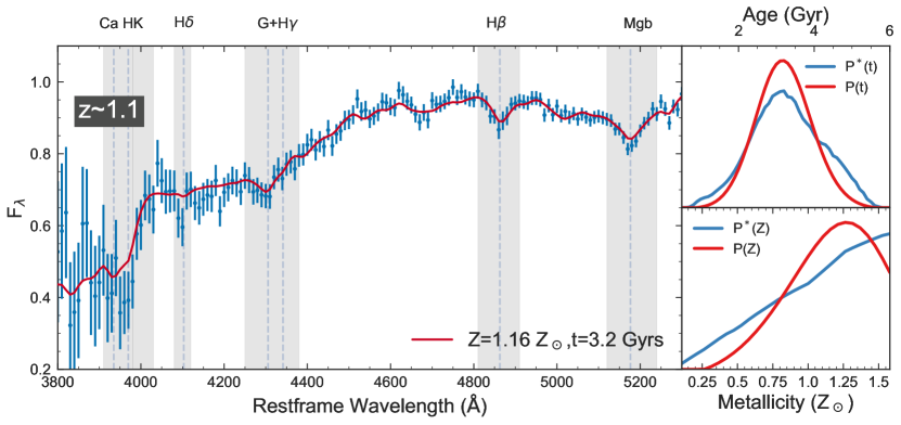
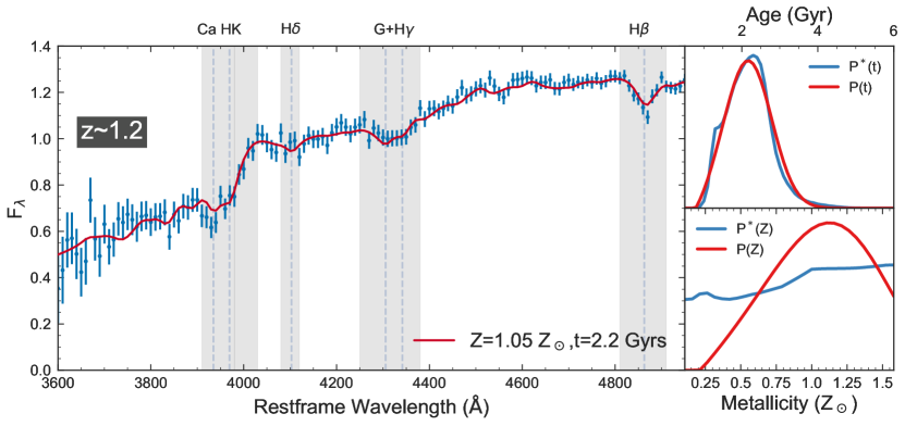
Figure 12: Top: Stacked spectra and posteriors for galaxies in the z $\sim$ 1.1 redshift subgroup. The main panel shows the stacked 1D G102 grism data against rest-frame wavelength. The sub-panels on the right show the stacked posteriors (blue:weighted stacking, red:“stack-smooth-iterate” method ) on light-weighted age ($t$) and metallicity ($Z$) derived using the method described in Section 5.2. The red-solid line in the main panel shows a model with the median $Z$ and $t$ taken from these individual-parameter posteriors (i.e., these are not best-fit models to the stack). Bottom: Same plots for the z $\sim$ 1.2 redshift subgroup of galaxies.

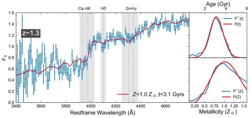
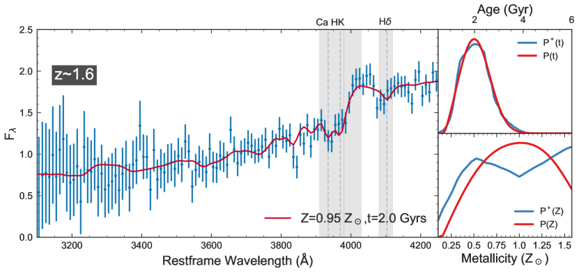
Figure 13: Same as Figure 12 for galaxies in the z $\sim$ 1.3 (top) and z $\sim$ 1.6 (bottom) galaxy subgroups.

From the stacked posteriors we derive median and 68%-tile ranges on the light weighted ages and metallicities for the galaxies in the different redshift subgroups. Based on our tests (in Appendix D) we interpret the 68%-tile distributions as an estimate of the intrinsic scatter in parent distribution of the population. Table 3 lists these values as well as the mass range and number of galaxies for each redshift subgroup.

Table 2: Measured parameters for individual galaxies from this work

ID	$z_{grism}$	Metallicity	Age	$\tau$	A(V)
		($Z_{\odot}$)	(Gyr)	(Gyr)	(Mag)
(1)	(2)	(3)	(4)	(5)	(6)
GND16758	$1.015_{-0.002}^{+0.002}$	$1.23_{-0.32}^{+0.25}$	$3.56_{-0.50}^{+0.76}$	$0.31_{-0.21}^{+0.24}$	$0.06_{-0.05}^{+0.08}$
GSD39241	$1.017_{-0.002}^{+0.002}$	$1.24_{-0.27}^{+0.23}$	$3.74_{-0.55}^{+0.75}$	$0.27_{-0.18}^{+0.22}$	$0.17_{-0.09}^{+0.11}$
GSD42221	$1.018_{-0.005}^{+0.005}$	$1.20_{-0.50}^{+0.27}$	$1.24_{-0.31}^{+0.85}$	$0.26_{-0.20}^{+0.67}$	$0.20_{-0.12}^{+0.18}$
GSD43615	$1.020_{-0.005}^{+0.002}$	$1.12_{-0.38}^{+0.31}$	$3.86_{-0.78}^{+0.90}$	$0.27_{-0.19}^{+0.24}$	$0.48_{-0.16}^{+0.20}$
GSD39170	$1.023_{-0.002}^{+0.002}$	$1.40_{-0.24}^{+0.13}$	$3.42_{-0.34}^{+0.31}$	$0.48_{-0.28}^{+0.14}$	$0.04_{-0.03}^{+0.04}$
GND37955	$1.027_{-0.002}^{+0.005}$	$1.24_{-0.54}^{+0.25}$	$2.67_{-0.36}^{+0.45}$	$0.68_{-0.33}^{+0.22}$	$0.63_{-0.25}^{+0.23}$
GSD45972	$1.041_{-0.002}^{+0.002}$	$0.73_{-0.23}^{+0.42}$	$3.48_{-0.77}^{+1.05}$	$0.27_{-0.18}^{+0.25}$	$0.08_{-0.06}^{+0.09}$
GSD39631	$1.057_{-0.010}^{+0.002}$	$0.64_{-0.29}^{+0.50}$	$3.56_{-0.90}^{+1.00}$	$0.25_{-0.18}^{+0.24}$	$0.19_{-0.11}^{+0.13}$
GSD47677	$1.117_{-0.005}^{+0.002}$	$1.05_{-0.47}^{+0.38}$	$3.11_{-0.67}^{+0.90}$	$0.30_{-0.21}^{+0.26}$	$0.30_{-0.16}^{+0.22}$
GND23435	$1.139_{-0.007}^{+0.005}$	$0.73_{-0.43}^{+0.57}$	$2.23_{-0.73}^{+0.65}$	$0.34_{-0.24}^{+0.34}$	$0.38_{-0.20}^{+0.27}$
GND34694	$1.145_{-0.002}^{+0.002}$	$1.12_{-0.39}^{+0.29}$	$2.21_{-0.47}^{+0.71}$	$0.18_{-0.12}^{+0.21}$	$0.25_{-0.13}^{+0.14}$
GND32566	$1.148_{-0.002}^{+0.005}$	$1.15_{-0.48}^{+0.31}$	$2.11_{-0.63}^{+0.39}$	$0.54_{-0.35}^{+0.31}$	$0.36_{-0.19}^{+0.24}$
GND23758	$1.161_{-0.002}^{+0.005}$	$0.60_{-0.45}^{+0.61}$	$2.10_{-0.25}^{+0.28}$	$1.02_{-0.24}^{+0.21}$	$0.90_{-0.14}^{+0.07}$
GSD38785	$1.169_{-0.002}^{+0.005}$	$0.80_{-0.53}^{+0.50}$	$2.47_{-0.56}^{+0.63}$	$0.43_{-0.29}^{+0.28}$	$0.29_{-0.16}^{+0.22}$
GND17070	$1.175_{-0.014}^{+0.005}$	$1.09_{-0.43}^{+0.34}$	$2.10_{-0.67}^{+0.50}$	$0.34_{-0.25}^{+0.33}$	$0.15_{-0.10}^{+0.14}$
GSD40476	$1.209_{-0.002}^{+0.002}$	$0.51_{-0.27}^{+0.45}$	$1.83_{-0.57}^{+0.68}$	$0.22_{-0.15}^{+0.28}$	$0.44_{-0.19}^{+0.24}$
GSD40597	$1.221_{-0.002}^{+0.002}$	$1.22_{-0.40}^{+0.25}$	$2.49_{-0.34}^{+0.21}$	$0.63_{-0.25}^{+0.16}$	$0.20_{-0.12}^{+0.14}$
GSD35774	$1.227_{-0.005}^{+0.002}$	$1.28_{-0.27}^{+0.21}$	$1.65_{-0.34}^{+0.52}$	$0.12_{-0.08}^{+0.11}$	$0.57_{-0.24}^{+0.26}$
GSD39805	$1.243_{-0.019}^{+0.051}$	$1.06_{-0.59}^{+0.38}$	$2.10_{-0.47}^{+0.36}$	$0.59_{-0.31}^{+0.27}$	$0.40_{-0.22}^{+0.29}$
GND21156	$1.249_{-0.002}^{+0.002}$	$0.83_{-0.34}^{+0.36}$	$2.20_{-0.52}^{+0.58}$	$0.26_{-0.17}^{+0.22}$	$0.31_{-0.14}^{+0.16}$
GND37686	$1.256_{-0.002}^{+0.001}$	$0.58_{-0.24}^{+0.43}$	$3.10_{-0.63}^{+0.78}$	$0.23_{-0.16}^{+0.24}$	$0.49_{-0.18}^{+0.20}$
GSD46066	$1.326_{-0.002}^{+0.012}$	$1.04_{-0.28}^{+0.31}$	$3.48_{-0.58}^{+0.57}$	$0.18_{-0.12}^{+0.17}$	$0.44_{-0.22}^{+0.28}$
GSD40862	$1.328_{-0.005}^{+0.002}$	$1.15_{-0.45}^{+0.30}$	$2.52_{-0.69}^{+0.72}$	$0.19_{-0.13}^{+0.19}$	$0.45_{-0.23}^{+0.27}$
GSD39804	$1.333_{-0.001}^{+0.005}$	$0.94_{-0.28}^{+0.37}$	$3.17_{-0.54}^{+0.67}$	$0.21_{-0.15}^{+0.20}$	$0.28_{-0.16}^{+0.21}$
GSD44620	$1.334_{-0.007}^{+0.005}$	$0.80_{-0.48}^{+0.54}$	$0.96_{-0.26}^{+0.53}$	$0.22_{-0.14}^{+0.33}$	$0.62_{-0.28}^{+0.25}$
GSD40623	$1.413_{-0.005}^{+0.019}$	$1.02_{-0.23}^{+0.29}$	$3.08_{-0.50}^{+0.56}$	$0.16_{-0.11}^{+0.16}$	$0.27_{-0.15}^{+0.19}$
GND21427	$1.506_{-0.022}^{+0.072}$	$0.91_{-0.46}^{+0.44}$	$2.43_{-0.60}^{+0.64}$	$0.25_{-0.18}^{+0.24}$	$0.40_{-0.21}^{+0.27}$
GSD40223	$1.595_{-0.005}^{+0.005}$	$0.81_{-0.42}^{+0.49}$	$1.82_{-0.48}^{+0.44}$	$0.47_{-0.22}^{+0.22}$	$0.48_{-0.24}^{+0.29}$
GSD41520	$1.605_{-0.002}^{+0.002}$	$0.97_{-0.49}^{+0.46}$	$1.98_{-0.55}^{+0.66}$	$0.18_{-0.12}^{+0.18}$	$0.73_{-0.20}^{+0.17}$
GSD39012	$1.612_{-0.024}^{+0.010}$	$0.75_{-0.43}^{+0.55}$	$1.87_{-0.53}^{+0.58}$	$0.45_{-0.27}^{+0.27}$	$0.42_{-0.23}^{+0.30}$
GSD44042	$1.612_{-0.002}^{+0.002}$	$1.28_{-0.85}^{+0.22}$	$2.33_{-0.28}^{+0.33}$	$0.47_{-0.20}^{+0.11}$	$0.22_{-0.13}^{+0.18}$

Note. — (1) Galaxy ID number in the GND or GSD 3D-HST catalog; (2) measured grism redshift; (3) median metallicity; (4) median light-weighted age; (5) median e-folding time for delayed $\tau$ SFH; (6) median A(V) for Calzetti dust law; all measurements provided with 68% confidence intervals; horizontal lines show the galaxies in each of the separate redshift subgroups

Table 3: Measured parameters for each redshift subgroup

Redshift group	Metallicity	Age	Mass Range	Sample Size
	($Z_{\odot}$)	(Gyr)	(log(M∗/M⊙))	(N)
(1)	(2)	(3)	(4)	(5)
z $\sim$ 1.1	$1.16_{-0.33}^{+0.26}$	$3.2\pm 0.7$	10.1–11.1	12
z $\sim$ 1.2	$1.05_{-0.36}^{+0.32}$	$2.2\pm 0.6$	10.6–11.2	9
z $\sim$ 1.3	$1.00_{-0.31}^{+0.31}$	$3.1\pm 0.6$	10.5–11.0	5
z $\sim$ 1.6	$0.95_{-0.40}^{+0.37}$	$2.0\pm 0.6$	10.7–11.1	5

Note. — Values on (light-weighted) age and metallicity correspond to the median and 68% confidence range for each parameter, which we interpret as an estimate of the intrinsic scatter in the subgroup (see text); The columns show (1) Redshift of the sub-group of the stacked posteriors; (2) metallicity; (3) light-weighted age, (4) Mass range of the galaxies in each of the samples; (5) number of galaxies in each redshift sub-group.

6 Discussion

Our dataset and analysis allow us to explore the correlations between stellar mass, (light-weighted) age, and metallicity in galaxies at $z>1$, much closer in time to the galaxies’ quenching time. We can use these to constrain both the SFHs and enrichment histories of these galaxies. In the sections that follow, we interpret the results of our modeling.

It is important to note that throughout (unless otherwise specified) all ages correspond to “light weighted” ages (see above) as these are better constrained because they correspond to the stellar populations that dominate the light in the galaxies’ spectra (when weighted by their luminosity). These are related to the parametric form of the SFHs through Equation 2, and different choices in this can impact the (light-weighted or mass-weighted) ages by $\sim$0.4 Gyr (e.g., Carnall et al. 2017). We will explore the effects of different SFHs in a future work.

6.1 The Ages and Metallicities of Quiescent Galaxy Populations from $z\sim 1.1$ to $1.6$

Generally, our modeling of the quiescent galaxies from z $\sim$ 1.1 to z $\sim$ 1.6 favor (light-weighted) ages of $\simeq$2–4 Gyr (with age increasing with decreasing redshift) and near Solar metallicities. Here, we comment on the values and quality of the model fits.

For each redshift subgroup, Figures 12 and 13 show the stacked posterior on the age and metallicity. The model fits in the Figures have metallicity and age equal to the median value from these stacked posteriors (that is, these are not best fit models to the stack). Rather, the posteriors are derived by stacking the posteriors of the individual galaxies in each redshift subgroup using the method in Section 5.2, and the data are the stacks of the individual galaxies (weighted by their inverse variance). The agreement between the models and data match is qualitatively quite good.

The z $\sim$ 1.1 subgroup has median parameter values of $Z=1.16\pm 0.29$ $Z_{\odot}$, $t_{L}=3.2\pm 0.7$ Gyr (Figure 12 top panel). The regions around H$\beta$ and Mg$b$ are particularly well reproduced by the model. This may be expected as the S/N of the data are highest in those regions and these features are age and metallicity sensitive. The model agrees well with the data at bluer wavelengths, but it does not capture all the apparent features. For example, the data show possible absorption at H$\delta$ that is not reproduced in the model. However, the G102 grism has less sensitivity at these wavelengths, reflected by the larger uncertainties on the data in this part of the spectrum, and the spectral regions at bluer wavelengths constrain the models less. Furthermore, we would have expected stronger H$\delta$ absorption to be accompanied by stronger H$\gamma$ absorption, which is not seen in the data (providing additional constraints on the models).

The z $\sim$ 1.2 sample has median parameter values of $Z=1.05\pm 0.34$ $Z_{\odot}$, $t_{L}=2.2\pm 0.6$ Gyr (Figure 12 bottom panel). Qualitatively, we see excellent agreement between the model and data, especially in the regions from the 4000 Å/Balmer break out past H$\beta$, and these features drive the constraints on the model parameters.

The z $\sim$ 1.3 sample has median parameter values of $Z=1.00\pm 0.31$ $Z_{\odot}$ and $t_{L}=3.1\pm 0.6$ Gyr (Figure 13 top panel). The 68%-tile confidence intervals on light-weighted age and metallicity are as tight as those at z $\sim$ 1.1 and z $\sim$ 1.2 samples (see Table 3), implying the shape of the continuum has important constraining power even as important features (like H$\beta$ and Mg$b$) shift out of the wavelength coverage. Most of the information constraining the models comes from the wavelength region of the 4000 Å break to the rest-frame $B$-band, where the S/N is highest.

The z $\sim$ 1.6 sample has median parameter values of $Z=0.95\pm 0.39$ $Z_{\odot}$, and $t_{L}=2.0\pm 0.6$ Gyr (Figure 13 bottom panel). The 68%-tile range on the light-weighted age is nearly as tight as for the lower redshift subgroups. The metallicity measurements place this group as slightly sub-solar, with a fairly broad 68%-tile range.

6.2 On the Star-Formation and Quenching Histories of Quiescent Galaxies at $z>1$,

Figure 14: The evolution of light-weighted age as a function of redshift. The small, colored data points show results for the individual $1<z_{grism}<1.8$ galaxies in our sample. Large colored data points correspond to median values derived from the stacked posteriors for redshift subgroup as labeled. Error bars show 68% confidence intervals. Other small (black) data points correspond to results from Mendel et al. (2015); Choi et al. (2014); Gallazzi et al. (2014); Whitaker et al. (2013); Fumagalli et al. (2016); Ferreras et al. (2018). Generally, quiescent galaxies have younger stellar populations at higher redshifts, where their light-weighted age has nearly a constant offset from the age of the universe. This agrees with predictions from the Millennium simulation (Henriques et al. 2015), where the shaded band shows the median and 68%-tile scatter in light-weighted ages of quiescent galaxies in their predictions.

Figure 15: Distribution of galaxy formation redshifts. The Left panel shows the derived formation redshifts, $z_{70}$ of quiescent galaxies as a function of observed redshift. The Right panel shows the distribution of median formation redshifts for our samples. The formation redshift, $z_{\mathrm{form}}$, corresponds to the redshift where the galaxies had formed more than 68% of their stellar mass (see Section 6.2). Here, we only include age measurements (shown in black) from studies which measured light-weighted ages. The quiescent galaxies at $1<z_{grism}<1.8$ in our sample have formation redshifts $z_{\mathrm{form}}>2-3$ nearly independent of observed galaxy redshift.

Figure 14 shows the measured (light-weighted) ages as a function of redshift for the galaxies in our sample. The Figure shows the median values and 68$\%$ confidence intervals on the ages for each quiescent galaxy in our sample, as well as the ages derived from the stacks for each redshift subgroup. Generally, galaxies in our sample have ages $2-4$ Gyr, where there is a trend that higher redshift galaxies have younger ages. In Figure 14 we also compare the (light-weighted) ages for the galaxies in our study to some other studies in the literature that also report ages. Comparing our derived age measurements to many other studies is complicated by the fact that there are different definitions and conventions of “age”. There are three widely used definitions of age: the instantaneous age of the stellar population model; mass-weighted ages, and light (luminosity-)weighted ages (we use the latter here). For a given (declining) SFH , the instantaneous age is the oldest as it measures the time since the onset of star-formation. Mass–weighted and light-weighted ages will be younger than instantaneous ages as they average over the mass (or light) of stars that continue to form after the initial burst of star-formation. As discussed above, the light-weighted ages are more robust against uncertainties in the SFH. For this reason we only show other results for light-weighted ages in Figure 15 as they are most directly comparable to the ones here.

The ages we derive for the galaxies in our sample tend to be larger than some other values for galaxies at similar redshift taken from the literature (cf. Whitaker et al. 2013; Mendel et al. 2015; Fumagalli et al. 2016). This may result from systematic effects owing to different definitions of age in previous studies, and the fact that we treat the metallicity as a free parameter. As seen in the right panel of Figure 11, the metallicity–age degeneracy shows that lower metallicity solutions push the median age higher (consistent with the offsets between our work and most literature studies). For example, Carnall et al. (2017) allow the metallicity to be free and find similar (mass-weighted) ages for quiescent galaxies in the same redshift range as our sample here.

Interestingly, the light-weighted ages we derive are consistent with predictions of ($r$–band light-weighted) from the semi-analytic model (SAM) based on the Millennium simulation from Henriques et al. (2015). Figure 14 shows the 68% scatter in ages from galaxies from this SAM selected to be quiescent (defined by sSFR$<10^{-10}$ yr^-1). This implies that the quenching epochs predicted in the models are consistent with the results we derive here for our sample. (We plan a more detailed comparison in a future study.)

Figure 14 also shows that the light-weighted ages of the quiescent galaxies in our sample have a nearly constant offset from the age of the Universe at the observed redshifts of the galaxies in our sample. This implies the galaxies all quenched at approximately the same time in the past. Figure 15 illustrates this by showing the formation redshift $z_{\mathrm{form}}$ for each galaxy in our sample (and showing galaxies from the literature for comparison). Indeed, the galaxies in our samples show a near constant formation redshift, $z_{\mathrm{form}}>2.5$.

We can relate $z_{\mathrm{form}}$ to the amount of stellar mass the galaxies had formed at this formation time. This requires integrating the SFHs, accounting for the light-weighted ages and mass losses from stellar evolution. This is not straight-forward: for example there is no analytical solution (to our knowledge) to the integral in Equation 2, owing to the dependence of $L(t^{*}-t)$ on light-weighted age, metallicity, and SFH. However, we can make an approximation as the ages of the quiescent galaxies in our samples are all in the regime where $t^{*}\gg\tau$ (where $t^{\ast}$ is the instantaneous age of the model and $\tau$ is the $e$-folding time constant of the SFR). In this case we compare $\langle t(t^{\ast},\tau)\rangle_{L}$ (the light-weighted age) to $\langle t(t^{\ast},\tau)\rangle$ (i.e., the mass-weighted age), which we define as

$$\langle t(t^{\ast},\tau)\rangle=\frac{\int_{0}^{t^{*}}\Psi(t,\tau)\ (t^{*}-t)\ dt}{\int_{0}^{t^{*}}\Psi(t,\tau)\ dt}$$ (12)

For the case where $t^{*}>\tau$ it will always be the case that

$$\langle t(t^{\ast},\tau)\rangle_{L}<\langle t(t^{\ast},\tau)\rangle.$$ (13)

For the case $t^{*}\gg\tau$, it can be shown that for delayed-$\tau$ SFHs, equation 12 reduces to

$$\langle t(t^{\ast}\gg\tau,\tau)\rangle\approx t^{*}-2\tau.$$ (14)

That is, the light-weighted age is always less than the (mass-weighted) age because for our galaxy sample the stellar populations fade monotonically. This leads to an upper bound on the light-weighted age, $\langle t(t^{\ast},\tau)\rangle_{L}$,

$$\langle t(t^{\ast},\tau)\rangle_{L}<t^{\ast}-2\tau.$$ (15)

Empirically, we find that Equation 15 holds for $\langle t(t^{\ast},\tau)\rangle_{L}$ $>$ 1.5 Gyr, and $t^{\ast}\geq 4\tau$. For younger light-weighted ages, there is a bias of $\lesssim$15% (so long as $t^{*}\geq 4\tau$ is satisfied).

Figure 16: Left panel: Mass–metallicity relation for quiescent galaxies at $1.0<z_{grism}<1.7$. The small, colored data points and error bars show the median values and 68%-tile range for the individual galaxies in our redshift subgroups, as labeled in the figure legend. The large colored data points show the metallicities from the stacked posteriors for each subgroup. The thick solid line shows a linear fit to the individual galaxies and the shaded region shows the 68%–tile bound. The dashed and dot–dashed lines show the mass-metallicity relation for quiescent galaxies from lower redshift samples (from SDSS at $z<0.22$, Gallazzi et al. (2005); and $z\sim 0.7$ from Gal14). We also include measurements of individual galaxies from Gal14 and Ferreras et al. (2018). Right panel: Histogram of the median metallicities for the galaxies in our $1.0<z_{grism}<1.7$ sub-groups. The majority of the probability density lies around $\approx Z_{\odot}$.

The stellar–mass formed for a SFH parameterized as a “delayed-$\tau$” model is then

$$M(t,\tau)=m(t,\tau)\ C\ \int_{0}^{t}t^{\prime}\ e^{-t^{\prime}/\tau}\ dt^{\prime}$$ (16)

where $m(t,\tau)$ is the fractional mass loss function (and depends on age, SFH and stellar population model). $C$ is a constant we can solve for by setting $t=t^{*}$ and $M(t^{*},\tau)=M_{obs}$ (the measured stellar mass).

Substituting in the value for $C$ leads to

$$M(t\ |\ M_{obs},t^{\ast},\tau)=\frac{m(t,\tau)\ M_{obs}\ \int_{0}^{t}\ t^{\prime}\ e^{-t^{\prime}/\tau}\ dt^{\prime}}{m(t^{*},\tau)\ \tau^{2}\ (1-e^{-t^{*}/\tau}[1+t^{*}/\tau])}$$ (17)

Using the approximation for $\langle t(t^{\ast},\tau)\rangle_{L}<t^{\ast}-2\tau$, we find a lower limit on the stellar mass formed at $\langle t(t^{\ast},\tau)\rangle_{L}$ (called the “quenching mass”, $M_{Q}$),

$$M_{Q}>M(t=2\tau)=\frac{0.6\ m(2\tau,\tau)\ M_{obs}}{m(t^{*},\tau)\ (1-e^{-t^{*}/\tau}[1+t^{*}/\tau])}$$ (18)

Finally, again applying the limit of $t^{*}\gg\tau$, we can approximate $M_{Q}$ to be

$$M_{Q}>0.6\times\frac{m(2\tau,\tau)}{m(t^{*},\tau)}\times M_{obs}$$ (19)

The values of $m$ are determined by the stellar population model, including the effects of the IMF. For a Salpeter IMF $M_{Q}>0.68$ $M_{obs}$, and for a Chabrier IMF $M_{Q}>0.75$ $M_{obs}$. Therefore, for the assumed SFHs, the galaxies in our sample would have formed $\gtrsim$70% of their stellar mass by the redshift that corresponds to their light-weighted ages, which we define as $z_{\mathrm{form}}$.

Both $z_{70}$ and $M_{Q}$ are related to the assumed star-formation history. To test how different parameterizations for this affect our light-weighted ages, we refit our galaxies with both $\tau$ and delayed $\tau$ models. The only effect seen on the light-weighted ages was a systematic shift (delayed $\tau$ models produce lower light-weighted ages). Using $\tau$-models rather than delayed-$\tau$ models increases the light-weighted ages and shifts the formation redshifts to $z_{\mathrm{form}}>4$.

Compared to the galaxies in our sample, quiescent galaxies at lower redshifts have lower formation redshifts (see Figure 15, and Mendel et al. 2015; Choi et al. 2014; Gallazzi et al. 2014; Whitaker et al. 2013; Fumagalli et al. 2016; Ferreras et al. 2018, although a direct comparison is complicated by the different definitions of “age” in some studies). This is likely a consequence of progenitor bias, where the progenitors of quiescent galaxies at $z<1$ are a mix of quiescent galaxies and some star-forming galaxies at $z>1$ (that quench at later time). Because some fraction of the population is star-forming at higher redshift, they will be younger at lower redshift and shift the mean formation redshift lower. Similarly, quiescent galaxies could become “younger” if they accrete enough mass through minor (dry) mergers of (quenched) lower mass galaxies with younger ages (see discussion in Choi et al. 2014).

Our results imply there should exist a population of massive quiescent galaxies at redshifts as high as $z>3$. Indeed, candidates of such galaxies have been identified (e.g., Renzini 2006; Guo et al. 2012; Spitler et al. 2014; Straatman et al. 2014; Merlin et al. 2018), where recent spectroscopic confirmation shows the rest-frame optical light strong Balmer absorption features (i.e., dominated by A-type stars), indicative of recent quenching (Glazebrook et al. 2017; Schreiber et al. 2018a).

We can gain insight into the evolution of these objects by comparing the (comoving) number densities of these massive galaxy candidates at $z>2$ to those in our sample. Figure 15 shows that roughly one-third of our sample experienced early quenching, with $z_{70}$ $>$ 3. Spitler et al. (2014) measure a number density when considering all massive galaxies ($\log M_{\ast}/M_{\odot}>10.6$) at $3<z<4$ of $5.1\times 10^{-5}$ Mpc^-3. We can compare this to number density of quiescent galaxies in our sample ($1<z_{grism}<1.8$) with $\log M/M_{\odot}>10.85$ (the higher mass here is needed to account for the $\sim 30\%$ growth expected as our estimates of the "formation redshift", $z_{70}$, correspond to the point where our galaxies had formed 70% of their mass). Using this mass limit we find a number density of $1.3(\pm 0.2)\times 10^{-4}$ Mpc^-3, where the uncertainty is purely Poissonian. Taking one-third of this number density (to account for the one-third of objects that quenched at $z_{70}>3$), this is consistent with the measured number density from Spitler et al. (2014), but it requires that $\approx$all of the massive galaxies at $z>3$ quench to account for the galaxies with high $z_{70}$ in our sample.

The rest of the galaxies quench at lower redshift ($2<z<3$, see Figure 15). Integrating the galaxy stellar mass functions from Tomczak et al. (2014), we find that quiescent galaxies with $\log M_{\ast}/M_{\odot}>10.6$ have a number density of $1.3\times 10^{-4}$ Mpc^-3. These are equal to the density number we derive for quiescent galaxies in our sample, showing we can account for all the population of quiescent galaxies we observe at $1<z<1.8$ (not even accounting for uncertainties or from changes in stellar mass through mergers, but see below). This evidence supports the $z_{70}$ values we derive.

6.3 The Mass–Metallicity Relation for Quiescent Galaxies at $z>1$

The CLEAR WFC3 G102 data allows us to measure stellar metallicities for quiescent galaxies at $z>1$. Because our sample is closer (in redshift) to the epoch when the galaxies quenched, we can better constrain their enrichment history.

Figure 16 shows the mass-metallicity relation for the quiescent galaxies in our sample at $1<z_{grism}<1.7$. The figure shows evidence that (1) quiescent galaxies at this redshift have near Solar Metallicities, and (2) that a mass–metallicity relationship for these quiescent galaxies is nearly unchanged from the $z\sim 0.1$ to $z>1$.

The mass-metallicity relation for $z\sim 1-1.7$ quiescent galaxies is either flat (no dependence) with stellar mass or slightly increasing with stellar mass. We fit a linear relation to the data of the form,

$$\log(Z_{*}/Z_{\odot})=A\log(M_{*}/10^{11}\ M_{\odot})+B$$ (20)

for all the $1<z_{grism}<1.7$ galaxies in our sample. This yielded a fit with $A=0.15\pm 0.13$, $B=0.08\pm 0.03$, with a covariance, $\sigma_{AB}=0.002$, which is illustrated as the shaded area in the figure.

The zero-point and shallow slope of the mass-metallicity relation show that the galaxies in our sample are consistent with Solar metallicity. Furthermore, Figure 16 shows that the stacked posteriors of galaxies in each redshift subgroup are strongly clustered around Solar metallicities, and that the distribution (histogram) of median metallicities for all the galaxies in our sample are likewise peaked around Solar metallicities. Therefore, we interpret this as strong evidence for Solar-metallicity enrichment in quiescent galaxies at $z\sim 1-1.7$.

In contrast, there is no evidence for evolution in the slope and zeropoint of the mass-metallicity relation for quiescent galaxies from $1\lesssim z\lesssim 1.7$ to $z\sim 0.2$. Figure 16 shows that the measurements for galaxies at $z<0.22$ from SDSS (Gallazzi et al. 2005) and at $z\sim 0.7$ (Gal14) are consistent with the same mass-metallicity relation we infer at $z>1$. (Similar results are found by Lonoce et al. 2015; Onodera et al. 2015; Ferreras et al. 2018). This is consistent with the assertion that these galaxies enriched rapidly while they formed their stars up to Solar metallicities, they have evolved passively since.

At higher redshift, $z>2$, there is some evidence that massive ($\log(M_{*}/M_{\odot})>11.0$) quiescent galaxies include objects with $\approx$Solar (and super-Solar) metallicities, as well as objects with less (sub-Solar metallicity) enrichment (Kriek et al. 2016; Toft et al. 2017; Morishita et al. 2018), with (in at least one case) evidence for super-Solar [$\alpha$/Fe] enrichment (e.g., Kriek et al. 2016). This could imply that at these epochs we are seeing the quenching of the cores of galaxies, which may evolve to higher metallicity at later times through mergers (see below, and discussion in Kriek et al. 2016). However, current constraints at $z>2$ are based on only a few (four) galaxies (highlighting the difficulty of these measurements) and larger galaxy samples are required.

Similarly interesting would be to study the evolution of the metallicity ([Fe/H]) and the $\alpha$-element enrichment ([$\alpha$/Fe]) in our galaxies. This is clearly an important problem given that massive quiescent galaxies at low redshifts show evidence for [$\alpha$/Fe] $>$ 0 (e.g., Thomas et al. 2010; Conroy et al. 2014), with some recent evidence at high redshift (e.g., Kriek et al. 2016; Steidel et al. 2016). This is likely related to their short SFHs combined with delay times in of Type Ia supernovae (e.g., Dahlen et al. 2012; Friedmann & Maoz 2018). Given that the $z\sim 1-1.7$ quiescent galaxies in our sample likely have similar histories to those at $z\sim 0$ (see discussion below), we may expect them to be similarly $\alpha$-enriched. We plan to study this in a future work.

6.4 Implications for Enrichment and Quenching of $z>1$ Quiescent Galaxies

Star-forming galaxies show a (gas-phase) mass-metallicity relation that evolves strongly with redshift. This contrasts strongly with the (lack of) evolution in the mass-metallicity relation for quiescent galaxies we find out to $1.0<z<1.7$. For example, the mass-metallicity relation for galaxies from SDSS at $z\sim 0.1$ derived from nebular emission lines shows that the gas-phase metallicity rises quickly with mass, and is Solar (or exceeds Solar) for the most massive galaxies (with stellar masses $\log M_{\ast}/M_{\odot}>10.5$, Tremonti et al. 2004; Andrews & Martini 2013). This evolves with redshift: at $z\sim 2.3$ the metallicities of star-forming galaxies at $\log(M_{\ast}/M_{\odot})$=10.5 are lower by about a factor of $\sim$2 compared to $z\sim 0.1$ (Tadaki et al. 2013; Zahid et al. 2014; Sanders et al. 2017, although this depends slightly on systematics owing to different metallicity indicators), and by about a factor of $\sim$3 at $z\sim 3.3$ (Onodera et al. 2016). This evolution persists even for absorption-line studies, where Gal14 report a similar offset in the stellar metallicity for star-forming galaxies at $z\sim 0.7$ at fixed stellar mass (in contrast to their mass-metallicity relation for quiescent galaxies which shows no evolution to $z\sim 0.7$).

What does it mean that the metallicities of quiescent galaxies at $1<z<1.7$ all favor near Solar metallicities? The lack of evolution in their mass-metallicity relation means that the progenitors of the galaxies in our sample presumably also had Solar metallicities at the time of quenching, $z_{70}\gtrsim 2.$. However, this makes their star-forming progenitors strong outliers in metallicity, offset from the gas–phase mass-metallicity relation observed at $z\sim 2.3$ and $z\sim 3.3$ for galaxies with stellar mass $\log M_{\ast}/M_{\odot}>10.5$ (Onodera et al. 2016; Sanders et al. 2017, see above). Observationally, there are few (if any) star-forming galaxies at these masses and redshifts with Solar metallicity that are candidates for the progenitors of the quiescent galaxies in our sample (this is assuming metallicity indicators used for quiescent and star forming galaxies are consistent, which is unclear).

Insight may be garnered from theory. In simulations of galaxies at these redshifts, the slope and scatter of the gas–phase mass-metallicity relation is a result of the combination of gas accretion, gas fraction, feedback, and metal-retention efficiency (Oppenheimer et al. 2012; Torrey et al. 2017). The slope of the gas-phase mass-metallicity relation is a result of mass-dependent gas accretion and feedback, resulting in lower metal retention efficiency for lower mass galaxies. This reproduces the observed evolution of the gas-phase mass-metallicity relation (e.g., Torrey et al. 2017).

The simulations show that at $z\sim 2$ the mean metallicity of massive galaxies is sub-Solar. However, the distribution extends to higher values and some galaxies have roughly Solar metallicity (Torrey et al. 2017). One explanation is that gas accretion has ceased in these galaxies (or slowed down, possibly as the galaxies are in the act of quenching, see below), and/or their metal retention efficiencies are higher (related to the fact that their escape velocities are larger), making it easier for them to enrich to higher metallicities faster. Interestingly, the lack of evolution in the observed mass-metallicity relation for quiescent galaxies out to $z>1$ could mean that these processes of galaxy quenching are redshift independent, which would set a requirement on simulations.

Why is it then that quiescent galaxies observed at nearly all redshifts have Solar metallicity? It could be that obtaining Solar metallicity is a symptom of the processes that lead to quenching and be related to the observational differences between quiescent and star-forming galaxies. One way to correlate the build-up of metals to quenching is by connecting the metal retention efficiency to galaxy feedback and galaxy size (Muratov et al. 2015; Christensen et al. 2016). Quiescent galaxies are known to have smaller effective radii compared to mass-matched star-forming galaxies (van der Wel et al. 2011), and this observation has led to theories such as the process of “compactification”, which relates sizes sizes to quenching (e.g., Dekel et al. 2009; Barro et al. 2013). Such scenarios could also lead to a natural connection between the high Solar metallicity and quenching in galaxies: as galaxies become more compact, the increase in their mass- and SFR-surface densities leads to stronger feedback, likely pushing the galaxy beyond the quenching point (Thompson et al. 2005; Barro et al. 2013); the increase in their escape velocities and SFR leads to higher metal production and retention (Ellison et al. 2008; Torrey et al. 2017). This is a plausible explanation for our observations, but it remains to be seen if simulations can reproduce the detailed values and evolution. For example, one prediction if the metal enrichment occurs prior to quenching is that more compact star-forming galaxies should likewise have higher metallicity (consistent with some results for galaxies in the SDSS, see Ellison et al. 2008). We plan to test this at higher redshift in a future study.

Regardless, if the Solar metallicities in our sample are correct, then their progenitors must exist somewhere. Some may be related to the compact star-forming galaxies discussed above (Barro et al. 2013). It is also possible that the time for galaxies to enrich from $\sim$1/3–1/2 $Z_{\odot}$ to $Z_{\odot}$ is very short-lived, in which case they may be very rare in surveys. For example, if quenching is tied to the process of “compaction”, the timescales could be $\ll 1$ Gyr (Zolotov et al. 2015), such that finding metal-rich star-forming galaxies in this stage is rare. This “rapid” phase would also be consistent with high [$\alpha$/Fe] abundances (e.g., Kriek et al. 2016, and we plan to test for this in future work). However, as surveys of $z>2$ galaxies become larger (Kriek et al. 2015), we expect them to include examples of this population.

Another possible explanation for the lack of metal-rich star-forming progenitors is that current samples of spectroscopically studied galaxies at $z\sim 2$ and 3 contain components of metal-enriched gas, but only in regions with heavy dust obscuration. In this case, the (rest-frame optical) spectra only probe the lower-metallicity gas (possibly diluted by recent inflows of pristine gas), yielding a mass-metallicity relation biased low. Alternatively, it may be that current spectroscopic studies of star-forming galaxies lack the progenitors of the quiescent galaxies in our samples entirely because the former are completely attenuated by dust. Massive, dusty star-forming galaxies are known to exist (e.g., Papovich et al. 2006; Casey et al. 2013; Spilker et al. 2014), with the space densities that connect them to quiescent galaxies (Spitler et al. 2014; Toft et al. 2014). Some dusty star-forming galaxies are observed to have compact gas reservoirs (Simpson et al. 2015; Tadaki et al. 2015), which likewise make them candidate progenitors to quiescent galaxies at lower redshifts. Future observations at at (rest-frame) near-IR to far-IR wavelengths (such as with the James Webb Space Telescope [JWST] and the Atacama Large Millimeter Array [ALMA]) may identify this galaxy population (and/or the higher- metallicity gas components in galaxies at these redshifts, see previous paragraph). It may also be possible to resolve these regions of high metallicity through higher angular resolution studies (e.g., with the Giant Segmented Mirror Telescopes [GSMTs] combined with adaptive optics).

7 Summary

In this work we used deep HST spectroscopy to constrain the metallicities and light-weighted ages of massive ($\log M_{\ast}/M_{\odot}\gtrsim 10$), quiescent galaxies at $1.0<z<1.8$. We selected 32 galaxies from existing HST and multi-wavelength imaging in the GOODS-N and -S fields also covered by our deep, 12–orbit WFC3/G102 grism pointings from CLEAR. For redshifts $1.0<z<1.8$ the data cover important stellar population features in the rest-frame optical, including the Ca HK feature, 4000 Å break, Balmer lines, Mg$b$, several other Lick indices and Fe I Iron lines, which are sensitive to stellar population age and metallicity. All galaxies are selected to have rest-frame optical colors ($U-V$ and $V-J$) indicative of quiescent stellar populations, so that we can use the HST grism data to study the relation between galaxy star-formation and enrichment histories and galaxy quenching.

We developed a method to forward model stellar population models, combining the grism dispersion model with the galaxy morphology to model accurately the galaxy spectra and contamination from spectra of nearby sources. We extracted 1D spectra from these models so they match the 1D spectra measured from the data. We validated this method by fitting these models to simulated data from which we are able to recover stellar population ages and metallicities. We showed that there are four redshift subgroups with median redshifts, z $\sim$ 1.1, z $\sim$ 1.2, z $\sim$ 1.3, z $\sim$ 1.6, which contain different spectral features in the G102 wavelength coverage, and we discussed the systematic differences and statistical uncertainties in the results for stellar population parameters for galaxies that fall in these redshift subgroups.

We then fit the suite of stellar population models to the 1D G102 grism data for each galaxy in our sample, taking into account the galaxies’ morphologies to correctly model the grism resolution. We first re-fit for galaxy redshifts using the grism data, and find small corrections from the photometric redshifts derived from broad-band photometry. The grism redshifts yield an accuracy of $\sigma_{z}\approx 0.005$ compared to the typical photometric redshift from broad-band photometry, $\sigma_{z}\approx 0.02-0.10$. Using the grism redshifts, we then fit the models to derive posterior likelihood distributions for metallicity and light-weighted age for each galaxy. We considered two sets of stellar population models: FSPS and BC03, but we argue the FSPS models are a better representation for these galaxies based on evidence from Bayes Factors derived from the fitting these models to all the galaxies. We then stack the posteriors for light-weighted ages and metallicities from the fits of stellar population models to each galaxy in each of the four redshift subgroups to derive constraints on the stellar population parameters for the galaxy populations.

Because we are observing the quiescent galaxies closer to their quenching epoch, our results place tighter constraints on their formation history than has generally been possible. Considering the full range of SFHs in our models, we derive light-weighted ages for the galaxies at $1.0<z<1.8$ that correspond to a “formation” redshift of $z_{70}>2$, with approximately one-third of the sample showing $z_{70}>3$. We show that for the SFHs, these formation redshifts correspond to the epoch when the galaxies had formed formed $\gtrsim 70$% of their stellar mass. The implication is that quiescent galaxies formed the bulk of their stellar mass early. This connects them to recently identified quiescent galaxies at redshifts as high as $z\sim 3-4$ (e.g., Glazebrook et al. 2017; Schreiber et al. 2018a).

We derive constraints on the metallicities of the quiescent galaxies at $1.0<z<1.8$, which show that these massive galaxies had enriched rapidly to approximately Solar metallicities as early as $z_{70}\sim 3$. We also show that a mass-metallicity relation exists for $1<z_{grism}<1.7$ quiescent galaxies, and that this is consistent with no evolution from $z\sim 1.7$ to $z<0.1$.

Logically, the star-forming progenitors of these galaxies must have been similarly enriched to approximately Solar metallicities prior to quenching. Because there are few galaxies (at any mass) at $z\sim 2-3$ with Solar gas-phase metallicities, the progenitors of the quiescent galaxies would be outliers in existing samples. This means there is something special about galaxies on the verge of quenching in the high redshift Universe: either they are more compact with higher metal retention efficiencies (possibly these are the blue-compact galaxies seen at $z>2$), very short lived phases ($\ll 1$ Gyr), or their progenitors are deeply attenuated by dust which current surveys (that select in the rest-frame optical, i.e., $H$-band or $K$-band) are biased against. It also may be that some combination of these effects are in play. The key to understanding the quenching of quiescent galaxies observed at $1\lesssim z\lesssim 1.7$ will be to identify their Solar-metallicity star-forming progenitors at $z>2-3$. Such studies will be possible in the future with JWST, ALMA, and the GSMTs.

Appendix A Results of fitting stellar population models to all sample galaxies

In this appendix we show the spectra for each galaxy along with the model fit from our analysis. In Figure 17 and 18 we show the 1D G102 grism data for all the galaxies in our sample. The red line in each figure shows the “median" model fit, the stellar population model with parameter values equal to the median values in Table 2. For each galaxy, the figures also show the joint posterior on the (light-weighted) age and metallicity from the stellar population model fitting.

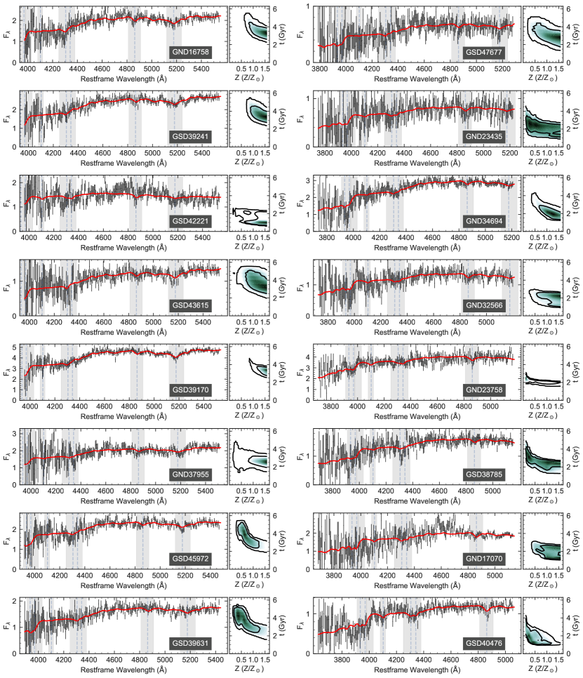
Figure 17: The data and model fits for the first 16 of the 31 galaxies in our sample. In the left hand panel of each subplot, the gray data points show the measured spectra (and uncertainties). The red lines show the model fits using median values for the parameters. The shaded regions correspond to the metallicity–age spectral features. The right hand panel of each subplot shows the metallicity and (light-weighted) age joint likelihoods. The legend shows the galaxy ID, and Table 2 gives the derived values for each model parameter for each galaxy.

Figure 18: Same as Figure 17 showing the remaining 15 of 31 galaxies in our dataset.

Appendix B Template Error Function

Figure 19: Distribution of the normalized residuals and the template error function. The top panel shows ($(F_{\lambda}-M)$ / $F_{\lambda}$) as a function of wavelength for all galaxies in the rest-frame, where $F_{\lambda}$ are the observed data (e.g., the G102 spectra) for each galaxy, $M$ is the best-fit model for each galaxy. The bottom panel shows the smoothed absolute normalized residuals (red, solid line; derived from the data in the top plot) along with the smoothed relative error (($\sigma_{\lambda}$ / $F_{\lambda}$), black dashed line, where $\sigma_{\lambda}$ are the measured uncertainties on the data) and the derived template error function ($E(\lambda)$, blue solid line) as described in the text.

To calculate our template error function we first find the best-fit model to the data for each galaxy (see Section 4.2). We then calculate a likelihood, $\mathcal{L}$, of the form

$$\mathcal{L}\propto\frac{1}{\sqrt{2\pi}s}\exp{(-x^{2}/(2s^{2}))}$$ (B1)

where $x=F_{\lambda}-M$ the difference between the data and model, and $s=\sqrt{\sigma_{F_{\lambda}}^{2}+(E(\lambda)F_{\lambda})^{2}}$ is the sum (in quadrature) of the errors on the data ($\sigma_{F_{\lambda}}$) and the “template error function”, $E(\lambda)$. We then take $d\mathcal{L}/dE(\lambda)=0$, and solve to find

$$E(\lambda)=\sqrt{\left(\frac{F_{\lambda}-M}{F_{\lambda}}\right)^{2}-\left(\frac{\sigma_{F_{\lambda}}}{F_{\lambda}}\right)^{2}}$$ (B2)

where the first term is the normalized residuals and the second term is the normalized error. We then follow the steps outlined in Brammer et al. (2008) to derive $E(\lambda)$.

The top panel in Figure 19 shows the distribution of $(F_{\lambda}-M)$ / $F_{\lambda}$ for all of our spectra. The bottom panel shows absolute median of this distribution as a function of wavelength, and shows the contributions from photometric uncertainties, and the error function, $E(\lambda)$. For wavelengths longward of $\gtrsim$3500 Å, there is only a small template error function ($\approx$5%). At shorter wavelengths, below $\sim$3500 Å, the template error function increases to as high as 30%, and may result of model uncertainties in the rest-frame UV. We include this error function in our fits, but in practice this has little effect on our results (as the data for rest-frame $\lesssim$3500 Å typically have lower S/N, so contribute little to the probably density).

Appendix C Bayesian Evidence Between the Stellar Population Models

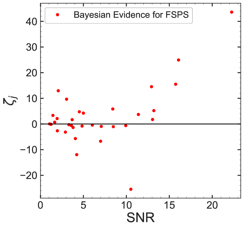
Figure 20: Distribution of Bayes-factor evidence ($\zeta_{j}$), for each galaxy $j$ in our sample, as a function of SNR. Positive (negative) values of $zeta_{j}$ denote galaxies with evidence against (in favor of) the BC03 models compared to the FSPS models.

In this study we performed model fits using two sets of composite stellar population synthesis models, those from FSPS and BC03 (see Section 4.1). In our analysis we favored results from FSPS, for the reason that it better fits the rest-frame wavelength region probed by the G102 data for our sample, approximately, $3000<\lambda_{\mathrm{rest}}/\hbox{\AA}<5800$. Similar results are found by Fum16 for quiescent galaxies at different redshifts with similar rest-frame wavelength coverage. Here, we use Bayesian evidence to support our use of the FSPS models in our conclusions.

We followed the description of the model selection process describe in (Salmon et al. 2016, see also Kass & Raftery 1995). We used the results from the fit of each set of models (BC03 and FSPS) to each galaxy in our sample using the same range of age and SFH parameters. For FSPS we use the same metallicity griding we use in our fitting, while for BC03 we use several of the metallicities made available ($Z=$[0.02, 0.2, 0.4, 1.0, 2.5] $Z_{\odot}$) . To compare the models, we consider all parameters, $\Theta$, as nuisance parameters. Marginalizing over the full parameter space includes probability contributions from all possible combinations of parameters for a given model, and the ratio of these then contains information about the relative probability for one model compared to the other. We may use this to derive the “odds” that favor one model over the other using the ratio of the model posteriors:

$$\frac{P(m_{1}|D)}{P(m_{2}|D)}=\frac{P(D|m_{1})}{P(D|m_{2})}\times\frac{P(m_{1})}{P(m_{2})}$$ (C1)

for the different stellar population models, $m_{1}$ and $m_{2}$, where $m_{i}$ is the i-th model (e.g., 1=FSPS, 2=BC03). In Equation C1, the term on the left-hand side is the ratio of posteriors (“Posterior Odds”). On the right-hand side, the last term is the ratio of priors (“Prior Odds”), and the first term is the so-called “Bayes Factor” (e.g., Jeffreys 1935; Kass & Raftery 1995), defined as

$$\mathrm{Bayes\ Factor}\equiv B_{12}=\frac{P(D|m_{1})}{P(D|m_{2})},$$ (C2)

where the values $P(D|m_{1,2})$ are the normalizations of the posteriors for each model, derived by marginalizing the posteriors over the full set of parameters,

$$P(D|m_{1,2})=\int_{\Theta}\ P(D|\Theta,m_{1,2})\ P(\Theta|m_{1,2})\ d\Theta.$$ (C3)

Conceptually, the Bayes factor is the ratio of the normalizations of the posteriors. A model that produces an overall better fit (over the full range of parameters, $\Theta$) will yield a higher normalization, and the ratio of these normalizations then indicates whether one model generally fits the data better, and is thus favored.

We quantified this using the definition of the Bayes-factor evidence ($\zeta$) (Kass & Raftery 1995), which is related to the Bayes factor by, $\zeta_{j}=2\ln B_{12,j}.$ Here the subscript $j$ corresponds to each galaxy in our sample. We then sum over all $\zeta_{j}$ to measure the significance of the Bayes factor evidence. If both models ($m_{1,2}$) fit the data equally well then $\Sigma\zeta_{j}=0$. A positive sum of the Bayes factor evidence ($\Sigma\zeta\ >\ 0$) shows evidence in favor of model 1 ($m_{1}$), while a negative sum of the Bayes factor evidence ($\Sigma\zeta\ <\ 0$) shows evidence towards model 2 ($m_{2}$). Kass & Raftery (1995) provide significance statements based on value of the Bayes factor evidence, which we adopt here.

We computed the Bayes factor for the FSPS and BC03 models for each galaxy in our sample, and then derived the overall Bayes factor evidence (the distribution of values are shown in Figure 20). Summing over $\zeta_{j}$ for all $j$ galaxies, we derived $\Sigma\ \zeta\ =\ 164$. This corresponds to “very strong” evidence (defined as $\Sigma\ \zeta>10$) against BC03 in favor of FSPS for the galaxies in our sample. We note that the grid of FSPS models is much finer in metallicity than BC03, and this could be a driving factor. We therefore recomputed the Bayes factor evidence using a set of FSPS models with the same metallicity griding as for BC03. In this case we derive $\zeta=96$, which is still “very strong” evidence for FSPS compared to BC03, and argues that for the galaxies in our sample the FSPS models provide a better overall fit to the data. For these reasons we adopt the FSPS for the conclusions in this study.

Appendix D Testing the “Stack–Smooth–Iterate” Method to Combine Parameter Likelihoods

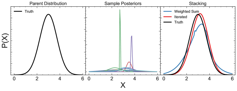
Figure 21: Test of our stacking method to recover a parent distribution. Panel 1 shows the true distribution, panel 2 show the randomly selected sample from distribution, and panel 3 displays a weighted sum of the sample posteriors along with the fully processed stacked posterior.

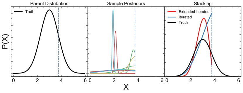
Figure 22: Test of our stacking method to recover a parent distribution when our parameter space does not cover the entirety of the parent distribution. Panel 1 shows the true distribution, panel 2 show the randomly selected sample from distribution, and panel 3 displays the fully processed stacked posterior with and without extending the parameter space.

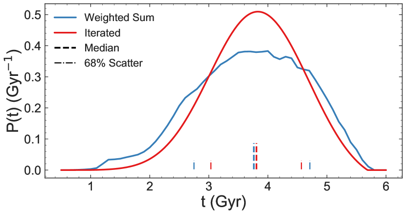
Figure 23: An example of the stacking method applied to the light-weighted age posteriors of our z $\sim$ 1.1 redshift group. The solid blue line shows the direct weighted sum (the result of direct stacking in the first step of the interaction using Equation 11). This yields the median and 68% confidence range illustrated by the blue dashed and dot-dashed lines. The solid red line shows the results after iterating. Because the iterations smooth over objects with sharply peaked likelihoods it yields a slightly tighter (and smoother) final likelihood. The red dashed and dot-dashed lines show the change in the median and 68% confidence range, respectively. We use the “stack-smooth-iterate” method to derive likelihoods from the galaxies in each of our redshift subgroups.

Here we test the stacking method described in Section 5.2 to see how well it reproduces a known true parent distribution. This process is illustrated in Figure 21. The test is done as follows: (1) We take a parent (Gaussian) distribution (shown in the first panel of Figure 21). (2) We randomly draw from it several data points (here we use 12 samplings to approximate a sample size similar to what we have in our z $\sim$ 1.1 redshift subgroup) with random errors (this is similar to a situation where some galaxies constrain their parameters better than others): this is illustrated in the middle panel of Figure 21. (3) Then we iteratively stack our sample posteriors to recover an approximation of the parent distribution following the method of Section 5.2. This is illustrated in the right panel of Figure 21. In that panel, the blue curve shows the recovered distribution after performing the weighted summation (the first step in the stacking process, which is identical to a weighted stack of the likelihoods). After the first step, the weighted distribution contains sharp peaks from objects with highly constrained likelihood functions. If these sharp peaks are not removed the iteration process will tend to follow the peaks, and the final product will be highly skewed. The red curve shown in panel 3 is the final product of the iterative stacking process. This included 20 iterations, although even a few iterations ($\sim$5) produce a good approximation of the correct distribution (and subsequent iterations approach an estimation of the truth distribution asymptotically). With a fixed sample size, n=12 in this case, the algorithm may converge to some estimate, but this will not be the true distribution. Convergence to the true distribution is only expected as the sample size gets larger.

One of the limitations of the stacking process described above is that it can fail in cases where the parameter space does not fully encompass the parent distribution ($\lesssim 90\%$ of the probability). When this occurs much of the probability mass will lie at the edge of the parameter space, and when the iterative stacking is applied the resulting distribution is driven to the edge (as seen in panel 3 of Figure 22). In order to resolve this we extend the parameter space artificially during the stacking process. This allows the distribution to fold over during the stacking process, preventing the distribution from sticking to the edge. This extended-iterative stack better reproduces the median value (though it often underestimates the confidence intervals).

Figure 23 shows the outcome of this “stack-smooth-iterate” process applied to our data for the galaxies in our z $\sim$ 1.1 sample. Here we see the differences between the weighted sum and iterated stack. There is a very slight shift in the median, $\sim$ 5% for metallicity and $\sim$ 1% for light-weighted age. The 68% confidence ranges are slightly tighter by $\sim$ 40% for metallicity and $\sim$ 10% for light-weighted age. The reason that the iterated distribution is “tighter” is that the presence of sharply peaked likelihoods from individual galaxies are smoothed in successive iterations as the method converges. We apply this method to all the galaxies in each of our redshift groups (z $\sim$ 1.1, z $\sim$ 1.2, z $\sim$ 1.3, z $\sim$ 1.6) to derive probability density functions parameters for each population.

References

- Andrews & Martini (2013) Andrews, B. H., & Martini, P. 2013, ApJ, 765, 140
- Bak & Statler (2000) Bak, J., & Statler, T. S. 2000, AJ, 120, 110
- Barro et al. (2013) Barro, G., Faber, S. M., Pérez-González, P. G., et al. 2013, ApJ, 765, 104
- Bertin & Arnouts (1996) Bertin, E., & Arnouts, S. 1996, A&AS, 117, 393
- Blakeslee et al. (2009) Blakeslee, J. P., Jordán, A., Mei, S., et al. 2009, ApJ, 694, 556
- Brammer et al. (2014) Brammer, G., Pirzkal, N., McCullough, P., & MacKenty, J. 2014, Time-varying Excess Earth-glow Backgrounds in the WFC3/IR Channel, Tech. rep.
- Brammer et al. (2008) Brammer, G. B., van Dokkum, P. G., & Coppi, P. 2008, ApJ, 686, 1503
- Brammer et al. (2012) Brammer, G. B., van Dokkum, P. G., Franx, M., et al. 2012, ApJS, 200, 13
- Bruzual & Charlot (2003) Bruzual, G., & Charlot, S. 2003, MNRAS, 344, 1000
- Calzetti et al. (2000) Calzetti, D., Armus, L., Bohlin, R. C., et al. 2000, ApJ, 533, 682
- Carnall et al. (2017) Carnall, A. C., McLure, R. J., Dunlop, J. S., & Davé, R. 2017, ArXiv e-prints, arXiv:1712.04452
- Casey et al. (2013) Casey, C. M., Chen, C.-C., Cowie, L. L., et al. 2013, MNRAS, 436, 1919
- Chabrier (2003) Chabrier, G. 2003, Publications of the Astronomical Society of the Pacific, 115, 763
- Choi et al. (2014) Choi, J., Conroy, C., Moustakas, J., et al. 2014, ApJ, 792, 95
- Christensen et al. (2016) Christensen, C. R., Davé, R., Governato, F., et al. 2016, ApJ, 824, 57
- Cleveland (1979) Cleveland, W. S. 1979, Journal of the American Statistical Association, 74, 829
- Conroy et al. (2014) Conroy, C., Graves, G. J., & van Dokkum, P. G. 2014, ApJ, 780, doi:10.1088/0004-637X/780/1/33
- Conroy & Gunn (2010) Conroy, C., & Gunn, J. E. 2010, ApJ, 712, 833
- Conroy et al. (2009) Conroy, C., Gunn, J. E., & White, M. 2009, ApJ, 699, 486
- Daddi et al. (2005) Daddi, E., Renzini, A., Pirzkal, N., et al. 2005, ApJ, 626, 680
- Dahlen et al. (2012) Dahlen, T., Strolger, L.-G., Riess, A. G., et al. 2012, ApJ, 757, 70
- Dekel et al. (2009) Dekel, A., Sari, R., & Ceverino, D. 2009, ApJ, 703, 785
- Eisenhardt et al. (2008) Eisenhardt, P. R. M., Brodwin, M., Gonzalez, A. H., et al. 2008, ApJ, 684, doi:10.1086/590105
- Ellison et al. (2008) Ellison, S. L., Patton, D. R., Simard, L., & McConnachie, A. W. 2008, ApJ, 672, L107
- Epanechnikov (1969) Epanechnikov, V. A. 1969, Theory of Probability and its Applications, 14, 153
- Erb et al. (2006) Erb, D. K., Shapley, A. E., Pettini, M., et al. 2006, ApJ, 644, 813
- Ferreras et al. (2018) Ferreras, I., Pasquali, A., Pirzkal, N., et al. 2018, ArXiv e-prints, arXiv:1805.03665
- Friedmann & Maoz (2018) Friedmann, M., & Maoz, D. 2018, ArXiv e-prints, arXiv:1803.04421
- Fumagalli et al. (2016) Fumagalli, M., Franx, M., van Dokkum, P., et al. 2016, ApJ, 822, 1
- Gallazzi et al. (2014) Gallazzi, A., Bell, E. F., Zibetti, S., Brinchmann, J., & Kelson, D. D. 2014, ApJ, 788, 72
- Gallazzi et al. (2005) Gallazzi, A., Charlot, S., Brinchmann, J., White, S. D. M., & Tremonti, C. A. 2005, MNRAS, 362, 41
- Glazebrook et al. (2017) Glazebrook, K., Schreiber, C., Labbé, I., et al. 2017, Nature, 544, 71
- Grogin et al. (2011) Grogin, N. A., Kocevski, D. D., Faber, S. M., et al. 2011, ApJS, 197, 35
- Guo et al. (2012) Guo, Y., Giavalisco, M., Cassata, P., et al. 2012, ApJ, 749, 149
- Henriques et al. (2015) Henriques, B. M. B., White, S. D. M., Thomas, P. A., et al. 2015, MNRAS, 451, 2663
- Iyer & Gawiser (2017) Iyer, K., & Gawiser, E. 2017, ApJ, 838, 127
- Jeffreys (1935) Jeffreys, H. 1935, Journal of the Royal Statistical Society, 98, 39
- Kass & Raftery (1995) Kass, R. E., & Raftery, A. E. 1995, Journal of the American Statistical Association, 90, 773
- Kawinwanichakij et al. (2017) Kawinwanichakij, L., Papovich, C., Quadri, R. F., et al. 2017, ApJ, 847, 134
- Koekemoer et al. (2011) Koekemoer, A. M., Faber, S. M., Ferguson, H. C., et al. 2011, ApJS, 197, 36
- Kriek et al. (2009) Kriek, M., van Dokkum, P. G., Labbé, I., et al. 2009, ApJ, 700, 221
- Kriek et al. (2006) Kriek, M., van Dokkum, P. G., Franx, M., et al. 2006, ApJ, 649, L71
- Kriek et al. (2015) Kriek, M., Shapley, A. E., Reddy, N. A., et al. 2015, The Astrophysical Journal Supplement Series, 218, 15
- Kriek et al. (2016) Kriek, M., Conroy, C., van Dokkum, P. G., et al. 2016, Nature, 540, 248
- Labbé et al. (2005) Labbé, I., Huang, J., Franx, M., et al. 2005, ApJ, 624, L81
- Lee et al. (2014) Lee, J. C., Pirzkal, N., & Hilbert, B. 2014, Flux Calibration Monitoring: WFC3/IR G102 and G141 Grisms, Tech. rep.
- Lee-Brown et al. (2017) Lee-Brown, D. B., Rudnick, G. H., Momcheva, I. G., et al. 2017, ApJ, 844, doi:10.3847/1538-4357/aa7948
- Lonoce et al. (2015) Lonoce, I., Longhetti, M., Maraston, C., et al. 2015, MNRAS, 454, 3912
- Lotz et al. (2017) Lotz, J. M., Koekemoer, A., Coe, D., et al. 2017, ApJ, 837, 97
- Luo et al. (2017) Luo, B., Brandt, W. N., Xue, Y. Q., et al. 2017, The Astrophysical Journal Supplement Series, 228, 2
- Madau & Dickinson (2014) Madau, P., & Dickinson, M. 2014, ARA&A, 52, 415
- Matteucci (1994) Matteucci, F. 1994, A&A, 288, 57
- Mendel et al. (2015) Mendel, J. T., Saglia, R. P., Bender, R., et al. 2015, ApJ, 804, L4
- Merlin et al. (2018) Merlin, E., Fontana, A., Castellano, M., et al. 2018, MNRAS, 473, 2098
- Momcheva et al. (2016) Momcheva, I. G., Brammer, G. B., van Dokkum, P. G., et al. 2016, ApJS, 225, 27
- Morishita et al. (2018) Morishita, T., Abramson, L. E., Treu, T., et al. 2018, ApJ, 856, L4
- Muratov et al. (2015) Muratov, A. L., Kereš, D., Faucher- Giguère, C.-A., et al. 2015, MNRAS, 454, 2691
- Muzzin et al. (2013) Muzzin, A., Marchesini, D., Stefanon, M., et al. 2013, ApJ, 777, 18
- Oke & Gunn (1983) Oke, J. B., & Gunn, J. E. 1983, ApJ, 266, 713
- Onodera et al. (2015) Onodera, M., Carollo, C. M., Renzini, A., et al. 2015, ApJ, 808, 161
- Onodera et al. (2016) Onodera, M., Carollo, C. M., Lilly, S., et al. 2016, ApJ, 822, 42
- Oppenheimer et al. (2012) Oppenheimer, B. D., Davé, R., Katz, N., Kollmeier, J. A., & Weinberg, D. H. 2012, MNRAS, 420, 829
- Pacifici et al. (2016) Pacifici, C., Kassin, S. A., Weiner, B. J., et al. 2016, ApJ, 832, 79
- Papovich et al. (2001) Papovich, C., Dickinson, M., & Ferguson, H. C. 2001, ApJ, 559, 620
- Papovich et al. (2011) Papovich, C., Finkelstein, S. L., Ferguson, H. C., Lotz, J. M., & Giavalisco, M. 2011, MNRAS, 412, 1123
- Papovich et al. (2006) Papovich, C., Moustakas, L. A., Dickinson, M., et al. 2006, ApJ, 640, 92
- Papovich et al. (2010) Papovich, C., Momcheva, I., Willmer, C. N. A., et al. 2010, ApJ, 716, 1503
- Papovich et al. (2012) Papovich, C., Bassett, R., Lotz, J. M., et al. 2012, ApJ, 750, 93
- Planck Collaboration et al. (2016) Planck Collaboration, Ade, P. A. R., Aghanim, N., et al. 2016, A&A, 594, A13
- Renzini (2006) Renzini, A. 2006, Annual Review of Astronomy and Astrophysics, 44, 141
- Riess et al. (2016) Riess, A. G., Macri, L. M., Hoffmann, S. L., et al. 2016, ApJ, 826, 56
- Salmon et al. (2015) Salmon, B., Papovich, C., Finkelstein, S. L., et al. 2015, ApJ, 799, 183
- Salmon et al. (2016) Salmon, B., Papovich, C., Long, J., et al. 2016, ApJ, 827, 20
- Salpeter (1955) Salpeter, E. E. 1955, ApJ, 121, 161
- Sanders et al. (2017) Sanders, R. L., Shapley, A. E., Kriek, M., et al. 2017, ArXiv e-prints, arXiv:1711.00224
- Schreiber et al. (2016) Schreiber, C., Elbaz, D., Pannella, M., et al. 2016, A&A, 589, A35
- Schreiber et al. (2018a) Schreiber, C., Koekemoer, A.and Nanayakkara, T., Kacprzak, G., et al. 2018a, A&A submitted
- Schreiber et al. (2018b) Schreiber, C., Labbé, I., Glazebrook, K., et al. 2018b, A&A, 611, A22
- Simha et al. (2014) Simha, V., Weinberg, D. H., Conroy, C., et al. 2014, ArXiv e-prints, arXiv:1404.0402
- Simpson et al. (2015) Simpson, J. M., Smail, I., Swinbank, A. M., et al. 2015, ApJ, 799, 81
- Skelton et al. (2014) Skelton, R. E., Whitaker, K. E., Momcheva, I. G., et al. 2014, ApJS, 214, 24
- Somerville & Davé (2015) Somerville, R. S., & Davé, R. 2015, ARA&A, 53, 51
- Spilker et al. (2014) Spilker, J. S., Marrone, D. P., Aguirre, J. E., et al. 2014, ApJ, 785, 149
- Spitler et al. (2014) Spitler, L. R., Straatman, C. M. S., Labbé, I., et al. 2014, ApJ, 787, L36
- Steidel et al. (2016) Steidel, C. C., Strom, A. L., Pettini, M., et al. 2016, ApJ, 826, 159
- Straatman et al. (2014) Straatman, C. M. S., Labbé, I., Spitler, L. R., et al. 2014, ApJ, 783, L14
- Straughn et al. (2011) Straughn, A. N., Kuntschner, H., Kümmel, M., et al. 2011, AJ, 141, 14
- Sullivan & Simcoe (2012) Sullivan, P. W., & Simcoe, R. A. 2012, PASP, 124, 1336
- Tadaki et al. (2013) Tadaki, K.-i., Kodama, T., Tanaka, I., et al. 2013, ApJ, 778, 114
- Tadaki et al. (2015) Tadaki, K.-i., Kohno, K., Kodama, T., et al. 2015, ApJ, 811, L3
- Thomas et al. (2005) Thomas, D., Maraston, C., Bender, R., & Mendes de Oliveira, C. 2005, ApJ, 621, 673
- Thomas et al. (2010) Thomas, D., Maraston, C., Schawinski, K., Sarzi, M., & Silk, J. 2010, MNRAS, 404, 1775
- Thompson et al. (2005) Thompson, T. A., Quataert, E., & Murray, N. 2005, ApJ, 630, 167
- Tilvi et al. (2016) Tilvi, V., Pirzkal, N., Malhotra, S., et al. 2016, ApJ, 827, L14
- Toft et al. (2014) Toft, S., Smolčić, V., Magnelli, B., et al. 2014, ApJ, 782, 68
- Toft et al. (2017) Toft, S., Zabl, J., Richard, J., et al. 2017, Nature, 546, 510
- Tomczak et al. (2014) Tomczak, A. R., Quadri, R. F., Tran, K.-V. H., et al. 2014, ApJ, 783, 85
- Torrey et al. (2017) Torrey, P., Vogelsberger, M., Marinacci, F., et al. 2017, ArXiv e-prints, arXiv:1711.05261
- Trager et al. (2000) Trager, S. C., Faber, S. M., Worthey, G., & González, J. J. 2000, AJ, 120, 165
- Tran et al. (2007) Tran, K.-V. H., Franx, M., Illingworth, G. D., et al. 2007, ApJ, 661, 750
- Tremonti et al. (2004) Tremonti, C. A., Heckman, T. M., Kauffmann, G., et al. 2004, ApJ, 613, 898
- van der Wel et al. (2011) van der Wel, A., Rix, H.-W., Wuyts, S., et al. 2011, ApJ, 730, 38
- van Dokkum & Brammer (2010) van Dokkum, P. G., & Brammer, G. 2010, ApJ, 718, L73
- van Dokkum et al. (2011) van Dokkum, P. G., Brammer, G., Fumagalli, M., et al. 2011, ApJ, 743, L15
- Weisz et al. (2014) Weisz, D. R., Dolphin, A. E., Skillman, E. D., et al. 2014, ApJ, 789, 147
- Whitaker et al. (2011) Whitaker, K. E., Labbé, I., van Dokkum, P. G., et al. 2011, ApJ, 735, 86
- Whitaker et al. (2013) Whitaker, K. E., van Dokkum, P. G., Brammer, G., et al. 2013, ApJ, 770, L39
- Whitaker et al. (2014) Whitaker, K. E., Franx, M., Leja, J., et al. 2014, ApJ, 795, 104
- Williams et al. (2009) Williams, R. J., Quadri, R. F., Franx, M., van Dokkum, P., & Labbé, I. 2009, ApJ, 691, 1879
- Windhorst et al. (2011) Windhorst, R. A., Cohen, S. H., Hathi, N. P., et al. 2011, ApJS, 193, 27
- Wu et al. (2018) Wu, P.-F., van der Wel, A., Gallazzi, A., et al. 2018, ApJ, 855, doi:10.3847/1538-4357/aab0a6
- Wuyts et al. (2007) Wuyts, S., Labbé, I., Franx, M., et al. 2007, ApJ, 655, 51
- Xue et al. (2016) Xue, Y. Q., Luo, B., Brandt, W. N., et al. 2016, ApJS, 224, 15
- Zahid et al. (2014) Zahid, H. J., Dima, G. I., Kudritzki, R.-P., et al. 2014, ApJ, 791, doi:10.1088/0004-637X/791/2/130
- Zolotov et al. (2015) Zolotov, A., Dekel, A., Mandelker, N., et al. 2015, MNRAS, 450, 2327