Classifying Multi-channel UWB SAR Imagery via Tensor Sparsity Learning Techniques

Abstract

Using low-frequency (UHF to L-band) ultra-wideband (UWB) synthetic aperture radar (SAR) technology for detecting buried and obscured targets, e.g. bomb or mine, has been successfully demonstrated recently. Despite promising recent progress, a significant open challenge is to distinguish obscured targets from other (natural and manmade) clutter sources in the scene. The problem becomes exacerbated in the presence of noisy responses from rough ground surfaces. In this paper, we present three novel sparsity-driven techniques, which not only exploit the subtle features of raw captured data but also take advantage of the polarization diversity and the aspect angle dependence information from multi-channel SAR data. First, the traditional sparse representation-based classification (SRC) is generalized to exploit shared information of classes and various sparsity structures of tensor coefficients for multi-channel data. Corresponding tensor dictionary learning models are consequently proposed to enhance classification accuracy. Lastly, a new tensor sparsity model is proposed to model responses from multiple consecutive looks of objects, which is a unique characteristic of the dataset we consider. Extensive experimental results on a high-fidelity electromagnetic simulated dataset and radar data collected from the U.S. Army Research Laboratory side-looking SAR demonstrate the advantages of proposed tensor sparsity models.

I Introduction

Over the past two decades, the U.S. Army has been investigating the capability of low-frequency, ultra-wideband (UWB) synthetic aperture radar (SAR) systems for the detection of buried and obscured targets in various applications, such as foliage penetration [1], ground penetration [2], and sensing-through-the-wall [3]. These systems must operate in the low-frequency spectrum spanning from UHF frequency band to L band to achieve both resolution and penetration capability. Although a lot of progress has been made over the years, one critical challenge that low-frequency UWB SAR technology still faces is discrimination of targets of interest from other natural and manmade clutter objects in the scene. The key issue is that that the targets of interest are typically small compared to the wavelength of the radar signals in this frequency band and have very low radar cross sections (RCSs). Thus, it is very difficult to discriminate targets and clutter objects using low-resolution SAR imagery.

I-A SAR geometry and image formation overview

Figure 1: Constant integration angle and multi-look SAR image formation via backprojection.

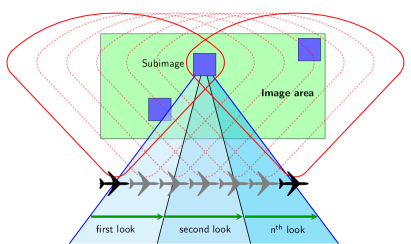
Figure 1 shows a typical side-looking SAR geometry where a vehicle or an airborne-based radar transmits wideband signals to the imaging area and measures the backscatter signals as it moves along an aperture. Let $s_{k}$ be the received range-compressed data received at $k^{\text{th}}$ aperture; the backprojection algorithm [4] computes the value for each SAR image pixel from the imaging area as follows:

$$P_{i}=\sum_{k=N_{i_{1}}}^{N_{i_{2}}}w_{k}*s_{k}(f(i,k)),$$ (1)

where $N_{i_{2}}-N_{i_{1}}+1$ is the total number of aperture records used for the coherent integration, $w_{k}$ is the weighting value at the $k^{\text{th}}$ aperture position, and $f(i,k)$ is the shift index to the signal $s_{k}$ for $i^{\text{th}}$ pixel at the $k^{\text{th}}$ aperture position. For a typical SAR image with $0^{\circ}$ aspect angle, $N_{i_{1}}$ and $N_{i_{2}}$ correspond to the angle values of $-\alpha/2$ and $\alpha/2$ to form a SAR image with an integration angle of $\alpha$. Note that for a true constant integration angle SAR image formation, $N_{i_{1}}$ and $N_{i_{2}}$ are computed for every pixel of the SAR image. However, for computational efficiency, a large image area is divided into smaller subimages. For each subimage, SAR image formation is computed using the $N_{i_{1}}$ and $N_{i_{2}}$ values derived from the geometry of the center of the subimage and the radar aperture. To exploit the aspect dependence information of target, instead of forming a single SAR image with $0^{\circ}$ aspect angle as described above with a single sector $[-\alpha/2,\alpha/2]$, we form multiple sectors to generate the corresponding SAR images at different aspect angles. For example, in our consecutive multi-look experiment, three SAR images are formed: left side image that covers sector $[-\alpha/2,\alpha/6]$, broadside image that covers sector $[-\alpha/6,\alpha/6]$, and right side image at sector $[\alpha/6,\alpha/2]$.

To achieve a constant cross-range resolution SAR image, a large image area is also divided into smaller subimages. Each subimage is formed using a different subset of aperture. For a constant integration angle, subimages at farther range would be integrated using a longer aperture than near-range subimages. The subimages are then mosaicked together to form a single large image that covers the area of interest. In consecutive multi-look SAR image processing mode, instead of generating a single SAR image, multiple SAR images are formed at different viewing angles to exploit the aspect angle dependent information from targets. Thus, each aperture for each subimage is further divided into smaller segments (either disjoint or overlapped) that are used to form consecutive multi-look SAR images as illustrated in Figure 1. The aspect angle dependence features from targets have been exploited in past research before using different techniques [5, 6, 4].

I-B Closely related works and motivation

UWB radar techniques have recently attracted increasing attention in the area of penetration and object detection, thanks to their usage in security applications and surveillance systems [7]. T. Sakamoto et al. [8] proposed fast methods for ultra-wideband (UWB) radar imaging that can be applied to a moving target. The technology has been also applied to 3-D imaging applications [9], human posture [10], human activity [11], vital sign [12], and liquid material [13] classification problems. In these papers, due to high dimensionality and small signal-to-ratio (SNR), the signals need to be preprocessed, e.g., dimensionality reduction and background subtraction, before being used to train a classifier. It has been shown that support vector machines usually provide the best performance [11, 13]. It is worth noting that in the aforementioned applications, objects are usually big (human) and captured from a relatively small distance. On the contrary, objects in our problem are relatively small and quite far from the radar.

In this paper, we consider the problem of discriminating and classifying buried targets of interest (metal and plastic mines, 155-mm unexploded ordinance [UXO], etc.) from other natural and manmade clutter objects (a soda can, rocks, etc.) in the presence of noisy responses from the rough ground surfaces for low-frequency UWB 2-D SAR images. For classification problems, sparse representation-based classification [14] (SRC) has been successfully demonstrated in other imagery domains such as medical image classification [15, 16, 17, 18], hyperspectral image classification [19, 20, 21], high-resolution X-band SAR image classification [22], video anomaly detection [23], and several others [24, 25, 26, 27, 28, 29, 30, 31]. However, in the low-frequency RF UWB SAR domain, although we have studied the feasibility of using SRC for higher-resolution 3-D down-looking SAR imagery [32], the application of SRC to low-frequency UWB 2-D SAR imagery has not been studied to date due to the aforementioned low-resolution issue. In this paper, we generalize the traditional SRC to address target classification using either a single channel (radar polarization) or multiple channels of SAR imagery. Additionally, we further propose a novel discriminative tensor sparsity framework for multi-look multi-channel classification problem, which is naturally suitable for our problem. In sparse representations, many signals can be expressed by a linear combination of a few basic elements taken from a “dictionary”. Based on this theory, SRC [14] was originally developed for robust face recognition. The main idea in SRC is to represent a test sample as a linear combination of samples from the available training set. Sparsity manifests because most of the nonzero components correspond to basic elements with the same class as the test sample.

Multi-channel SRC has been investigated before in medical images [16, 18]. In these papers, one dictionary for each channel is formed from training data with locations of all channels of one training point being the same in all dictionaries. Then intuitively, when sparsely encoding each channel of a new test point using these dictionaries, we obtain sparse codes whose active (nonzero) elements tend to happen at the same locations in all channels. In other words, active elements are simultaneously located at the same location across all channels. This intuition is formulated based on $l_{0}$ pseudo-norm, which is solved using a modified version of simultaneous orthogonal matching pursuit (SOMP) [33]. The cost function is nonconvex, and hence, it is difficult to find the global solution. Furthermore, when more constraints involved, there is no straightforward way to extend the algorithm. In this paper, we proposed another way of formulating the simultaneity constraint based on the $l_{12}$ norm, which enforces the row sparsity of the code matrix (in tensor form, we call it tube sparsity). The newly convex optimization problem can be solved effectively using the fast iterative shrinkage thresholding algorithm (FISTA) [34]. We also propose other different tensor sparsity models for our multi-channel classification problems.

It has been shown that learning a dictionary from the training samples instead of concatenating all of them as a dictionary can further enhance performance of sparsity-based methods. On one hand, the training set can be compacted into a smaller dictionary, reducing computational burden at the test time. On the other hand, by using dictionary learning, discriminative information of different classes can be trained via structured discriminative constraints on the dictionary as well as the sparse tensor code. A comprehensive study of discriminative dictionary learning methods with implementations is presented at [26, 35]. These dictionary learning methods, however, are all applied to single-channel problem where samples are often represented in form of vectors. While multi-channel signals can be converted to a long vector by concatenating all channels, this trivial modification not only leads to the curse of dimensionality of high-dimensional space, but also possibly neglects cross-channel information, which might be crucial for classification. In this paper, we also propose a method named TensorDL, which is a natural extension of single-channel dictionary learning frameworks to multi-channel dictionary learning ones. Particularly, the cross-channel information will be captured using the aforementioned simultaneity constraint.

Naturally, when a radar carried by a vehicle or aircraft moves around an object of interest, it can capture multiple consecutive views of that object (see Fig. 1). Consequently, if the multi-look information is exploited, the classification accuracy will be improved. While the multi-look classification problem has been approached before by SRC-related methods [22, 25], none of these works uses the relative continuity of different views. We propose a framework to intuitively exploit this important information. More importantly, the optimization problem corresponding to this structure can be converted to the simultaneous sparsity model by using an elegant trick that we call ShiftSRC. Essentially, a tensor dictionary is built by circularly shifting an appropriate amount of a single-channel dictionary. When we sparsely code the multi-look signals using this tensor dictionary, the tensor sparse code becomes tube sparsity.

I-C Contributions

The main contributions of this paper are as follows:

1. A framework for simultaneously denoising and classifying 2-D UWB SAR imagery. Subtle features from targets of interest are directly learned from their SAR imagery. The classification also exploits polarization diversity and consecutive aspect angle dependence information of targets.

2. A generalized tensor discriminative dictionary learning (TensorDL) is also proposed when more training data involved. These dictionary learning frameworks are shown to be robust even with high levels of noise.

3. A relative SRC framework (ShiftSRC) is proposed to deal with multi-look data. Low-frequency UWB SAR signals are often captured at different views of objects, depending on the movement of the radar carriers. These signals contain uniquely important information of consecutive views. With ShiftSRC, this information will be comprehensively exploited. Importantly, a solution to the ShiftSRC framework can be obtained by an elegant modification on the training dictionary, resulting in a tensor sparse coding problem, which is similar to a problem proposed in contribution 1).

The remainder of this paper is organized as follows. Section II presents different tensor sparsity frameworks and the discriminative tensor dictionary learning scheme for multi-channel classification problems. The ShiftSRC for multiple-relative-look and solutions to all proposed frameworks are also presented in this section. Section III shows extensive experimental results on a simulated dataset for several scenarios. An experiment with a realistic dataset is also included. Section IV concludes the paper.

II Sparse representation-based classification

II-A Notation

Scalars are denoted by italic letters and may be either lower or uppercase, e.g., $d,N,k$. Vectors and matrices are denoted by bold lowercase ($\mathbf{x,y}$) and bold upper case ($\mathbf{X,Y}$), respectively. In this paper, we also consider 3-D tensors (tensors for short) whose dimensions are named row, column, and channel. A tensor with only one column will be denoted by a bold, lowercase, calligraphic letter ($\mathbcal{x},\mathbcal{y}$). Tensors with more than one column will be denoted by an bold, uppercase, calligraphic letters ($\mathbfcal{X},\mathbf{Y},\mathbfcal{D}$).

For any tensor $\mathbfcal{M}$, let $\mathbfcal{M}^{(t)}$ be its $t$-th channel. For convenience, given two tensors $\mathbfcal{M},\mathbfcal{N}$, the tensor multiplication $\mathbfcal{P}=\mathbfcal{M}\mathbfcal{N}$ is considered channel-wise multiplication, i.e., $\mathbfcal{P}^{(t)}=\mathbfcal{M}^{(t)}\mathbfcal{N}^{(t)}$. For a tensor $\mathbfcal{M}$, we also denote the sum of square of all elements by $\|\mathbfcal{M}\|_{F}^{2}$ and the sum of absolute values of all elements by $\|\mathbfcal{M}\|_{1}$. Tensor addition/subtraction simply represents element-wise addition/subtraction. Each target sample is represented by a UWB SAR image formed using either a single (using co-pol) or multiple polarization (using both co-pol and cross-pol) channels. Thus, one target sample is denoted by $\mathbcal{y}\in\mathbb{R}^{d\times 1\times T}$, where $d$ is the total number of image pixels and $T$ is the number of polarization channels. A collection of $N$ samples is denoted by $\mathbf{Y}\in\mathbb{R}^{d\times N\times T}$.

Consider a general classification problem with $C$ different classes. Let $\mathbfcal{D}_{c}(1\leq c\leq C)$ be the collection of all training samples from class $c$, $\mathbfcal{D}_{0}$ be the collection of samples in the shared class, and $\mathbfcal{D}=[\mathbfcal{D}_{1},\dots,\mathbfcal{D}_{C},\mathbfcal{D}_{0}]$ be the total dictionary with the concatenation being done at the second dimension (column). In our problem, the shared class can be seen as the collection of ground images.

II-B Classification scheme

Using the definition of tensor multiplication, a sparse representation of $\mathbcal{y}$ using $\mathbfcal{D}$ can be obtained by solving

$$\mathbcal{x}=\arg\min_{\mathbcal{x}}\frac{1}{2}\|\mathbcal{y}-\mathbfcal{D}\mathbcal{x}\|_{F}^{2}+\lambda g(\mathbcal{x})$$ (2)

where $\lambda$ is a positive regularization parameter and $g(\mathbcal{x})$ is a function that encourages $\mathbcal{x}$ to be sparse. Denote by $\mathbcal{x}^{i}$ the sparse coefficient of $\mathbcal{y}$ on $\mathbfcal{D}_{i}$. Then, the tensor $\mathbcal{x}$ can be divided into $C+1$ tensor parts $\mathbcal{x}^{1},\mathbcal{x}^{2},\dots,\mathbcal{x}^{C},\mathbcal{x}^{0}$.

After solving the sparse coding problem (2), shared features (grounds in our problem) are eliminated by taking $\bar{\mathbcal{y}}=\mathbcal{y}-\mathbfcal{D}_{0}\mathbcal{x}^{0}$. Then the identity of one sample $\mathbcal{y}$ can be determined by the dictionary that provides the minimum residual:

$$\text{identity}(\mathbcal{y})=\min_{i\in\{1,2,\dots,C\}}\|\bar{\mathbcal{y}}-\mathbfcal{D}_{i}\mathbcal{x}^{i}\|^{2}_{2}$$ (3)

Confuser detection: In practical problems, the set of confusers is not limited to the training set. A confuser can be anything that is not a target; it can be solely the ground or a capture of an unseen object. In the former case, the test signal can be well represented by using only the ground $\mathbfcal{D}_{0}$, while in the latter case, the sparse representation assumption is no longer valid. Therefore, one test signal $\mathbcal{y}$ is classified as a confuser if one of following three conditions is satisfied: i) it is not sparsely interpreted by the total dictionary $\mathbfcal{D}$; ii) it has the most active elements in the sparse code locating at $\mathbcal{x}^{0}$; and iii) it is similar to known confusers.

II-C Generalized sparse representation-based classification

Figure 2: Different sparsity constraints on the coefficient tensor $\mathbcal{x}$.

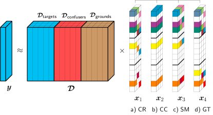
In SRC [14] where only one channel is considered, $g(\mathbcal{x})$ is simply a function that forces sparsity as $l_{0}$- or $l_{1}$-minimization. $l_{1}$-minimization is often used since it leads to a convex optimization problem with tractable solutions. In the following, we present two natural extensions of SRC for multi-channel cases. We also proposed two tensor sparse representation methods that can enhance classification accuracy by exploiting cross-channel information. These four generalized SRC methods are as follows.

a) Apply a sparsity constraint on each column of the coefficient tensor $\mathbcal{x}$, no cross-channel constraint.

We can see that this is similar to solving $T$ separate sparse coding problems, each for a polarization channel. The classification rule is executed based on the sum of all the squares of the residuals. We refer to this framework as SRC-cumulative residual or SRC-CR (CR in the short version). (See Figure 2a with sparse tensor $\mathbcal{x}_{1}$). The sparse code corresponding to the $t^{\text{th}}$ channel, $\mathbcal{x}^{(t)}$, is computed via the traditional $l_{1}$-minimization:

$$\mathbcal{x}^{(t)}=\arg\min_{\mathbcal{x}^{(t)}}\frac{1}{2}\|\mathbcal{y}^{(t)}-\mathbfcal{D}^{(t)}\mathbcal{x}^{(t)}\|_{2}^{2}+\lambda\|\mathbcal{x}^{(t)}\|_{1}$$ (4)

which can be solved effectively using FISTA [34], ADMM [37], etc., algorithms or the SPAMS toolbox [38].

b) Concatenate all channels.

The most convenient way to convert a multi-channel problem to a single-channel problem is to concatenate all $T$ channels of one signal to obtain a long vector. By doing so, we have the original SRC framework with $l_{1}$-norm minimization. After solving the sparse coding problem, if we break the long vectors and rearrange them back to tensor forms, then the tensor sparse coefficients $\mathbcal{x}$ can be formed by replicating the one-channel sparse coefficient at all channel (see Figure 2b with sparse tensor $\mathbcal{x}_{2}$). From this tensor viewpoint, the code tensor $\mathbcal{x}$ will have few active “tubes”; moreover, all elements in a tube are the same. We refer to this framework as SRC-concatenation or SRC-CC (CC in the short version).

The optimization problem in SRC-CC and its solution are very straightforward. First, we stack all channel dictionaries into a long one: $\hat{\mathbfcal{D}}=[\mathbfcal{D}^{(1)};\mathbfcal{D}^{(2)};\dots;\mathbfcal{D}^{(T)}]$ (symbol ‘;’ represents the concatenation in the first dimension). Then for every test signal, we also stack all of its channels to form a long vector: $\hat{\mathbcal{y}}=[\mathbcal{y}^{(1)};\mathbcal{y}^{(2)};\dots;\mathbcal{y}^{(T)}]$. The optimization problem (2) becomes the traditional $l_{1}$ regularization problem:

$$\mathbcal{x}=\arg\min_{\mathbcal{x}}\frac{1}{2}\|\hat{\mathbcal{y}}-\hat{\mathbfcal{D}}\mathbcal{x}\|_{2}^{2}+\lambda\|\mathbcal{x}\|_{1}$$ (5)

then also can be solved by aforementioned methods.

c) Use a simultaneous model.

Similar to the SHIRC model proposed in [16, 18], we can impose one constraint on active elements of tensor $\mathbcal{x}$ as follows: $\mathbcal{x}$ also has few nonzero tubes as in SRC-CC; however, elements in one active tube are not necessarily the same. In other words, the locations of nonzero coefficients of training samples in the linear combination exhibit a one-to-one correspondence across channels. If the $j$-th training sample in $\mathbfcal{D}^{(1)}$ has a nonzero contribution to $\mathbcal{y}^{(1)}$, then for $t\in\{2,\dots,T\}$, $\mathbcal{y}^{(t)}$ also has a nonzero contribution from the $j$-th training sample in $\mathbfcal{D}^{(t)}$. We refer to this framework as SRC-Simultaneous or SRC-SM (SM in the short version). (See Figure 2c with sparse tensor $\mathbcal{x}_{3}$). To achieve this requirement, we can impose on the tensor $\mathbcal{x}_{3}$ (with one column and T channels) the $l_{1,2}$-minimization constraint, which is similar to the row-sparsity constraint applied on matrices in [22].

Remarks: While SHIRC uses $l_{0}$-minimization on $\mathbcal{x}$ and applies the modified SOMP [33], our proposed SRC-SM exploits the flexibility of $l_{1,2}$-regularizer since it is convex, and easily modified when more constraints are present (e.g., non-negativity). In addition, it is more efficient especially when dealing with problems of multiple samples at input.

Concretely, the optimization problem of SRC-SM can be written in the form

$$\mathbcal{x}=\arg\min_{\mathbcal{x}}\frac{1}{2}\|\mathbcal{y}-\mathbfcal{D}\mathbcal{x}\|_{F}^{2}+\lambda\sum_{k=1}^{K}\|\text{vec}(\mathbcal{x}_{k::})\|_{2}$$ (6)

where $\mathbcal{x}_{k::}$ denotes the $k^{\text{th}}$ tube of the tensor code $\mathbcal{x}$ and $K$ is the total column of the dictionary $\mathbfcal{D}$, and $\text{vec}(\mathbcal{x}_{k::})$ is the vectorization of the tube $\mathbcal{x}_{k::}$. This problem is similar to the joint sparse representation (JSRC) problem proposed in [22] except that SRC-SM enforces tube-sparsity instead of the row-sparsity. Details of the algorithm that solves  are described in Section II-F.

d) Use a group tensor model.

Intuitively, since one object is ideally represented by a linear combination of the corresponding dictionary and the shared dictionary, it is highly likely that number of active (tensor) parts in $\mathbcal{x}$ is small, i.e., most of $\mathbcal{x}^{1},\dots,\mathbcal{x}^{C},\mathbcal{x}^{0}$ are zero tensors. This suggests us a group tensor sparsity framework as an extension of [39] that can improve the classification performance, which is referred to as SRC-GT (GT in the short version). The visualization of this idea is shown in Figure 2d.

The optimization problem of SRC-GT is similar to (6) with a slight difference in the grouping coefficients:

$$\mathbcal{x}=\arg\min_{\mathbcal{x}}\frac{1}{2}\|\mathbcal{y}-\mathbfcal{D}\mathbcal{x}\|_{F}^{2}+\lambda\sum_{c=1}^{C+1}\|\text{vec}(\mathbcal{x}^{c})\|_{2}$$ (7)

where $C+1$ is the total number of classes (including the shared ground class), and $\text{vec}(\mathbcal{x}^{c})$ is the vectorization of the group tensor $\mathbcal{x}^{c}$. Solution to this problem will be discussed next.

The overall algorithm of generalized SRC applied to multi-channel signals in the presence of a shared class is shown in Algorithm 1.

Algorithm 1 Generalized SRC with a shared class

function identity$(\mathbcal{y})$ =

          $\leavevmode\nobreak\ \leavevmode\nobreak\ \leavevmode\nobreak\ \leavevmode\nobreak\ \leavevmode\nobreak\ \leavevmode\nobreak\ \leavevmode\nobreak\ \leavevmode\nobreak\ \leavevmode\nobreak\ \leavevmode\nobreak\ \text{GENERALIZED\_SRC}(\mathbcal{y},\mathbfcal{D},\lambda,g(\bullet),\varepsilon,\tau)$

     INPUT:

$\mathbcal{y}\in\mathbb{R}^{d\times 1\times T}$ – a test sample;

$\mathbfcal{D}=[\mathbfcal{D}_{1},\mathbfcal{D}_{2},\dots,\mathbfcal{D}_{C},\mathbfcal{D}_{0}]\in\mathbb{R}^{d\times K\times T}$ – the total dictionary with the shared dictionary $\mathbfcal{D}_{0}$;

$g(\bullet)$ – the sparsity constraint imposed on sparse codes.

$\lambda\in\mathbb{R}^{+}$ – a positive regularization parameter;

$\varepsilon,\tau$ – positive thresholds.

     OUTPUT: the identity of $\mathbcal{y}$.

     1. Sparsely code $\mathbcal{y}$ on $\mathbfcal{D}$ via solving:

$${\mathbcal{x}}=\arg\min_{\mathbcal{x}}\{\|\mathbcal{y}-\mathbfcal{D}\mathbcal{x}\|_{F}^{2}+\lambda g(\mathbcal{x})\}$$ (8)

     2. Remove the contribution of the shared dictionary:

$$\bar{\mathbcal{y}}=\mathbcal{y}-\mathbfcal{D}_{0}\mathbcal{x}^{0}.$$

     3. Calculate the class-specific residuals :

$$r_{c}=\|\bar{\mathbcal{y}}-\mathbfcal{D}_{c}\mathbcal{x}^{c}\|_{2},\forall c=1,2,\dots,C.$$

     4. Decision:

     if $\displaystyle\min_{c}(r_{c})>\tau$ (an unseen object) or $\|\bar{\mathbcal{y}}\|_{2}<\varepsilon$ (a ground) then

         $\mathbcal{y}$ is a confuser.

     else

         $\displaystyle\text{identity}(\mathbcal{y})=\arg\min_{c}\{r_{c}\}$

     end if

end function

II-D Dictionary learning for tensor sparsity

As a natural extension, we can extend the tensor sparsity models to dictionary learning ones. Most of dictionary learning methods focus on a single-channel signal, which is not suitable for models with cross-channel information. In this work, we extend single-channel dictionary learning methods to multi-channel dictionary ones by applying aforementioned tensor sparsity constraints.

In single-channel, most of discrimination dictionary learning methods, such as FDDL [40], DLSI [41], DFDL [17], LRSDL [26], etc., have a cost function that is of the form

$$\bar{J}_{\mathbf{Y}}(\mathbf{D},\mathbf{X})=\bar{f}_{\mathbf{Y}}(\mathbf{D},\mathbf{X})+\lambda\bar{g}(\mathbf{X})$$ (9)

where $\bar{g}(\mathbf{X})$ is a function enforcing the sparsity of $\mathbf{X}$, and $\bar{f}_{\mathbf{Y}}(\mathbf{D},\mathbf{X})$, which includes fidelity and discriminant terms, is a function of $\mathbf{D},\mathbf{X}$ and depends on the training samples $\mathbf{Y}$.

One straightforward extension of these single-channel models to a multi-channel case is to apply the first term $f_{\mathbf{Y}}(\mathbf{D},\mathbf{X})$ to each channel and join all channels by a sparsity constraint represented by $g(\mathbf{X})$. Naturally, $g(\mathbf{X})$ can be one of four presented cross-channel sparsity constraints. Concretely, the overall cost function would be in the form

$${J}_{\mathbf{Y}}(\mathbfcal{D},\mathbfcal{X})={f}_{\mathbf{Y}}(\mathbfcal{D},\mathbfcal{X})+\lambda g(\mathbfcal{X})$$ (10)

where $f_{\mathbf{Y}^{(t)}}(\mathbfcal{D}^{(t)},\mathbfcal{X}^{(t)})=\bar{f}_{\mathbf{Y}^{(t)}}(\mathbfcal{D}^{(t)},\mathbfcal{X}^{(t)})$ and $g(\mathbfcal{X})$ is one of {CR, CC, SM, GT} sparsity constraints.

In this paper, we particularly focus on extending FDDL [40] to the multi-channel case. FDDL is a special case of LRSDL [26] without an explicit shared dictionary. FDDL is chosen rather than LRSDL since in our problem, the shared dictionary, e.g., grounds, is already separated out. We also adopt fast and efficient algorithms proposed in the dictionary learning toolbox DICTOL [35] to update each channel of the dictionary $\mathbfcal{D}$. Also, the sparse code tensor $\mathbfcal{X}$ is updated using FISTA [34] algorithm, which is discussed in Section II-F.

The proposed cross-channel dictionary learning method is named TensorDL suffixed by CR, CC, SM, or GT when different sparsity constraints are applied on $\mathbfcal{X}$.

Figure 3: Tensor sparsity with relative views.

II-E Tensor sparsity with multiple relative looks

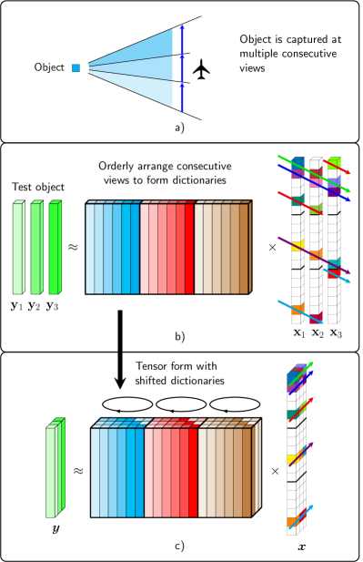
In realistic situations, objects might be captured at different angles instead of only one. Moreover, these are often consecutive angles that a plane or a vehicle can capture (see Figure 3a left) while moving around objects. Based on this observation, in the training phase, we collect data from different views of objects, as in Figure 3a right, and orderly arrange them into dictionaries for each object, as illustrated in Figure 3b. The test objects, which are often captured at different relative views $\mathbf{y}_{1},\mathbf{y}_{2},\mathbf{y}_{3}$, are then sparsely coded by the whole dictionary.

Intuitively, if $\mathbf{x}_{1}$ is the sparse code of the first view $\mathbf{y}_{1}$ with only few active elements, then the sparse code $\mathbf{x}_{2}$ of the next view $\mathbf{y}_{2}$ will be active at locations shifted by one. Similarly, active locations in $\mathbf{x}_{3}$ of the third view will be shifted by two compared to $\mathbf{x}_{1}$, and so on. In this case, active coefficients form a “stair”, as illustrated in Figure 3b right.

The sparse coding problem with the “stair” sparsity is a novel problem and has not been addressed before. In this paper, we propose a method called ShiftSRC to convert this problem to a previously known problem. The central idea is that if we stack all views into a tensor and “circularly shift” the ordered dictionary by one to the left at each view, then the obtained tensor code will be a tensor with active elements forming a “tube” sparsity (see Figure 3c). The solution to this problem is similar to the solution of SRC-SM as stated in this paper.

II-F Solution to optimization problems

Both optimization problems (6) and (7) have the form

$$\mathbcal{x}=\arg\min_{\mathbcal{x}}\{F(\mathbcal{x})\equiv f(\mathbcal{x})+\lambda g(\mathbcal{x})\},$$ (11)

where

• $g(\mathbcal{x})$ is sum of norm 2, then it is a continuous convex function and nonsmooth.

• $f(\mathbcal{x})=\frac{1}{2}\|\mathbcal{y}-\mathbfcal{D}\mathbcal{x}\|_{F}^{2}$ is a continuous convex function of the type $C^{1,1}$, i.e., continuously differentiable with a Lipschitz continuous gradient $L$:

  $$\|\nabla f(\mathbcal{x}_{1})-\nabla f(\mathbcal{x}_{2})\|_{F}\leq L\|\mathbcal{x}_{1}-\mathbcal{x}_{2}\|_{F}\leavevmode\nobreak\ \leavevmode\nobreak\ \text{for every}\leavevmode\nobreak\ \mathbcal{x}_{1},\mathbcal{x}_{2}.$$

We observe that, with these properties, the optimization problem (11) can be solved by FISTA [34]. There are three main tasks in FISTA:

1. Calculating $\nabla f(\mathbcal{x})$, which can be easily computed as

$$\nabla f(\mathbcal{x})=\mathbfcal{D}^{T}(\mathbfcal{D}\mathbcal{x}-\mathbcal{y}).$$

where each channel of $\mathbfcal{D}^{T}$ is the transpose of the corresponding channel of $\mathbfcal{D}$.

Algorithm 2 Tensor sparse coding by FISTA[34]

function ${\mathbcal{x}}$ = TENSOR_SC($\mathbcal{y},\mathbfcal{D},\mathbcal{x}_{\text{init}},\lambda$).

     1. Calculate

$$\mathbfcal{A} =\mathbfcal{D}^{T}\mathbfcal{D},\leavevmode\nobreak\ \leavevmode\nobreak\ \leavevmode\nobreak\ \mathbf{b}=\mathbfcal{D}^{T}\mathbcal{y}$$

$$L =\max_{t=1,2,\dots,T}(\lambda_{\max}(\mathbfcal{A}^{(t)}))$$

     2. Initialize $\mathbcal{x}_{0}=\mathbcal{x}_{\text{init}}$, $\mathbcal{w}_{1}=\mathbcal{x}_{0}$, $j=1,t_{1}=1$

     while non convergence and $j<j_{\max}$ do

         3. Calculate gradient: $\mathbcal{g}=\mathbfcal{A}\mathbcal{w}_{j}-\mathbcal{y}.$

         4. Calculate $\mathbcal{u}=\mathbcal{w}_{j}-\mathbcal{g}/L.$

         5. If SRC-SM, $\mathbcal{x}_{j}$ is the solution of (14); if SRC-GT, $\mathbcal{x}_{j}$ is the solution of (16).

         6. $t_{j+1}=(1+\sqrt{1+4t_{j}^{2}})/2$

         7. $\mathbcal{w}_{j+1}=\mathbcal{x}_{j}+\frac{t_{j}-1}{t_{j+1}}(\mathbcal{x}_{j}-\mathbcal{x}_{j-1})$

         8. $j=j+1$

     end while

     9. OUTPUT: $\mathbcal{x}=\mathbcal{x}_{j}$

end function

2. Calculating a Lipschitz constant of $\nabla f(\mathbcal{x})$. For our function $f$, we can choose

$$L=\max_{t=1,2,\dots,T}\left\{\lambda_{\max}\left((\mathbfcal{D}^{(t)})^{T}\mathbfcal{D}^{(t)}\right)\right\}$$ (12)

where $\lambda_{\max}$ is the maximum eigenvalue of a square matrix.

3. Solving a suboptimization problem of the form

$$\mathbcal{x}=\arg\min_{\mathbcal{x}}\left\{\frac{1}{2}\|\mathbcal{x}-\mathbcal{u}\|_{F}^{2}+\eta g(\mathbcal{x})\right\}$$ (13)

with $\eta=\frac{\lambda}{L}$.

For SRC-SM, problem (13) has the form

$$\mathbcal{x}=\arg\min_{\mathbcal{x}}\left\{\frac{1}{2}\|\mathbcal{x}-\mathbcal{u}\|_{F}^{2}+\eta\sum_{k=1}^{K}\|\text{vec}(\mathbcal{x}_{k::})\|_{2}\right\}$$

$$=\arg\min_{\mathbcal{x}}\left\{\sum_{k=1}^{K}\left(\frac{1}{2}\|\mathbcal{x}_{k::}-\mathbcal{u}_{k::}\|_{2}^{2}+\eta\|\text{vec}(\mathbcal{x}_{k::})\|_{2}\right)\right\}$$ (14)

Each problem in (14) is a minimum $l_{2}$-norm minimization with solution being

$$\mathbcal{x}_{k::}=\max\left\{1-\frac{\eta}{\|\text{vec}(\mathbcal{u}_{k::})\|_{2}},0\right\}\mathbcal{u}_{k::},\forall k=1,2,\dots,K.$$ (15)

Similarly, for SRC-GT, problem (13) can be written as

$$\mathbcal{x}=\arg\min_{\mathbcal{x}}\left\{\frac{1}{2}\|\mathbcal{x}-\mathbcal{u}\|_{F}^{2}+\eta\sum_{c=1}^{C+1}\|\text{vec}(\mathbcal{x}^{c}\|_{2}\right\}$$

$$=\arg\min_{\mathbcal{x}}\left\{\sum_{c=1}^{C+1}\left(\frac{1}{2}\|\mathbcal{x}^{c}-\mathbcal{u}^{c}\|_{2}^{2}+\eta\|\text{vec}(\mathbcal{x}^{c})\|_{2}\right)\right\}$$ (16)

with solution being:

$$\mathbcal{x}^{c}=\max\left\{1-\frac{\eta}{\|\text{vec}(\mathbcal{u}^{c})\|_{2}},0\right\}\mathbcal{u}^{c},\forall c=1,\dots,C+1.$$ (17)

Figure 4: Sample images of five targets and five clutter objects. T1 = M15 anti-tank mine, T2 = TM62P3 plastic mine, T5 = 155-mm artillery shell, C1 = soda can, C2 = rocks, C3 = rocks, C4 = rocks, C5 = rocks. a) Targets under smooth ground surface. b) Targets under rough ground surface (easy case, scale = 1). c) Targets under rough ground surface (hard case, scale = 5). d) Confusers under smooth ground surface. e) Confusers under rough ground surface (easy case, scale=1). f) Confusers under rough ground surface (hard case, scale=5).

A step by step description of SRC-SM and SRC-GT algorithms are given in Algorithm 2.

III Experimental results

Figure 5: Visualization of decomposed signals (HH polarization) after doing sparse coding. Row 1: the original clean signals. Row 2: the corresponding noisy signals with the interference of grounds. Row 3: reconstructed signal after sparse coding. Row 4: separated noises.

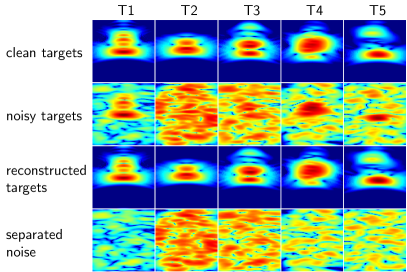
In this section, we apply the proposed models to the problem of classifying objects of interest. Extensive results are presented on simulated and real-life datasets. A MATLAB toolbox for the tensor sparsity methods presented in this paper is available at [42].

Table I: Overall average classification (%) of different methods on different polarization combinations, with or without the non-negativity constraint.

	Separate targets					All targets
	VV	HH	VV+HH	HH+HV	ALL	VV	HH	VV+HH	HH+HV	ALL
SVM	62.17	74.47	65.00	77.77	70.33	83.68	89.36	83.36	66.36	79.78
SRC-CR	76.32	83.43	86.26	85.93	82.95	86.22	91.64	87.14	91.28	90.64	without non-negativity constraint
SRC-CC	76.32	83.43	79.47	86.21	79.93	86.22	91.64	87.96	92.98	81.80
SRC-SM	76.32	83.43	81.07	86.52	85.87	86.22	91.64	89.66	95.12	94.14
SRC-GT	69.79	78.79	77.83	85.12	81.75	81.90	88.40	87.28	91.86	90.46
SRC-CR	79.05	89.41	79.85	88.52	84.92	86.32	92.98	87.48	94.86	94.26	with non-negativity constraint
SRC-CC	79.05	89.41	83.99	92.27	85.11	86.32	92.98	89.20	93.82	87.08
SRC-SM	79.05	89.41	85.62	90.85	89.36	86.32	92.98	90.00	96.82	96.00
SRC-GT	75.55	88.97	81.85	90.57	87.28	84.16	90.32	88.10	94.58	94.12

III-A Electromagnetic (EM) Simulation data

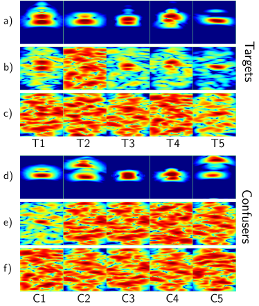
SRC is applied to a SAR database consisting of targets (metal and plastic mines, 155-mm unexploded ordinance [UXO], etc.) and clutter objects (a soda can, rocks, etc.) buried under rough ground surfaces. The electromagnetic (EM) radar data is simulated based on the full-wave computational EM method known as the finite-difference, time-domain (FDTD) software [43], which was developed by the U.S. Army Research Laboratory (ARL). The software was validated for a wide variety of radar signature calculation scenarios [44, 45]. Our volumetric rough ground surface grid – with the embedded buried targets – was generated by using the surface root- mean-square (rms) height and the correlation length parameters. The targets are flush buried at 2-3 cm depth. In our experiments, the easiest case of rough ground surface in our experiments, the surface rms is 5.6 mm and the correlation length is 15 cm. The SAR images of various targets and clutter objects are generated from EM data by coherently integrated individual radar return signals along over a range of aspect angles. The SAR images are formed using the backprojection image formation [46] with an integration angle of $30^{\circ}$. Figure 4a shows the SAR images (using vertical transmitter, vertical receiver – VV – polarization) of some targets that are buried under a perfectly smooth ground surface. Each target is imaged at a random viewing aspect angle and an integration angle of $30^{\circ}$. Figures 4b and  4c show the same targets as Figure 4a, except that they are buried under a rough ground surface (the easiest case corresponds to ground scale/noise level = 1 and harder case corresponds to noise level = 5). Similarly, Figures 4d, 4e, and 4f show the SAR images of some clutter objects buried under a smooth and rough surface, respectively. For training, the target and clutter object are buried under a smooth surface to generate high signal-to-clutter ratio images. We include 12 SAR images that correspond to 12 different aspect angles ($0^{\circ},30^{\circ},\dots,330^{\circ}$) for each target type. For testing, the SAR images of targets and confusers are generated at random aspect angles and buried under rough ground surfaces. Various levels of ground surface roughness are simulated by selecting different ground surface scaling factors when embedding the test targets under the rough surfaces. Thus, the resulting test images are very noisy with a very low signal-to-clutter ratio. Each image is a polarization signal of object which is formed by one of transmitter-receiver setups: vertical-vertical (VV), horizontal-horizontal (HH), or horizontal-vertical (HV). Each data sample of one object is represented by either i) one SAR image using data from one co-pol (VV, HH) channel or ii) two or more images using data from co-pol (VV, HH) and cross-pol (HV) channels. For each target type, we tested 100 image samples measured at random aspect angles.

III-B Denoised signal visualization

We construct the dictionary $\mathbfcal{D}=\left[\begin{matrix}\mathbfcal{D}_{t},\mathbfcal{D}_{c},\mathbfcal{D}_{c}\end{matrix}\right]$ of all three polarizations, with $\mathbfcal{D}_{t},\mathbfcal{D}_{c},\mathbfcal{D}_{g}$ being dictionaries of targets, confusers, and grounds, respectively. The sub-dictionary $\mathbfcal{D}_{o}=\left[\begin{matrix}\mathbfcal{D}_{t},\mathbfcal{D}_{c}\end{matrix}\right]$ can be seen as the dictionary of the objects of interest. For a noisy signal $\mathbcal{y}$, we first solve the following problem:

$$\mathbcal{x}=\arg\min_{\mathbcal{x}}\|\mathbcal{y}-\mathbfcal{D}\mathbcal{x}\|_{F}^{2}+\lambda g(\mathbcal{x})$$ (18)

where $g(\mathbcal{x})$ is the proposed SM constraint. The sparse tensor code $\mathbcal{x}$ is then decomposed into two parts, $\mathbcal{x}^{o}$ and $\mathbcal{x}^{\text{g}}$. The latter can be considered coefficients corresponding to the ground dictionary $\mathbfcal{D}_{g}$. The original signal can be approximately decomposed into two parts: $\mathbfcal{D}_{g}\mathbcal{x}^{g}$ as separated noise, and $\mathbfcal{D}_{o}\mathbcal{x}^{o}$ as the denoised signal. Visualization of these signals are shown in Figure 5. We can see that the tensor framework successfully decomposes noisy signals into a clean part and a ground signal. These results show the potential of the proposed tensor sparsity frameworks for classification.

III-C Overall classification accuracy

Figure 6: Classification accuracy (%) with different noise levels and different polarization combinations for the separate-target scenario.

We apply four methods presented in II-C to different combinations of three polarizations: VV, HH, VV+HH, HH+HV, and VV+HH+HV (or ALL), and also compare these results with those obtained by a support vector machine (SVM) using the libsvm library [47]. SVM was also applied to classify UWB signals [13, 11]. The training set comprises all five target sets, four out of five confuser sets (each time we leave one confuser set out, which is meant to be unseen), and the ground set. While all confuser sets can be seen as one class – confuser class – there are two ways of organizing target sets. First, each of five targets is considered one class in case the identity of each target is crucial (we name this scenario separate-target with five target classes and one confuser class). Second, if we only need to know whether an object of interest is a target or not, we can consider all five targets as one class and its corresponding name is all-target with one target class and one confuser class. We also consider two families of the sparse coding problem, one with and one without the non-negativity constraint on the sparse code $\mathbcal{x}$ in each of the tensor sparse coding methods. Each experiment is conducted 10 times and their results are reported as the average number. Parameters in each method are chosen by a 5-fold cross-validation procedure. In this experiment, all test samples are corrupted by small noise, i.e., the noise level is set to one. In our experiments, we use overall classification accuracy as the performance metric, which computes percentage of correctly classified samples over total test samples across all classes.

Overall classification accuracies of different methods on different polarization combinations are reported in Table I. From the table, a few inferences can be made:

• SRC-related methods with non-negative sparse coefficients perform better than those without this constraint. In addition, SVM is outperformed by all other methods in all tasks.

• SRC-SM provides the best results in all combinations for both the separate-target and all-target scenarios. The best accuracies in both cases are significantly high with slightly over 90% in the six-class classification problem and nearly 97% in the binary classification problem.

• If only one polarization is used, SRC-CR, SRC-CC, and SRC-SM have identical results, since all of them are basically reduced to traditional SRC in this case. Additionally, these three methods slightly outperform SRC-GT in this scenario.

• If only one polarization can be obtained, HH always outperforms VV and by a significant margin. Additionally, the HH+VV combination often worsens the results versus using HH alone.

• If the same method is used on different combinations, the best results are mostly obtained by the combination of HH and HV polarizations in both the separate-target and all-target scenarios.

III-D Effect of noise levels on overall accuracy

The results in the previous section are collected in the presence of small corruption (noise level is only 1). In real problems, objects of interest are, deliberately or not, buried under extremely rough surfaces in order to fool classifiers. In this section, we conduct an experiment to see how each method performs when the level of corruption increases in the separate-target scenario.

Classification results of five different methods on different polarization combinations and different noise levels are shown in Figure 6. First of all, similar trends to small corruption can be observed in that SRC-SM shows best performance in all cases with bigger gaps occurring at high levels of noise. In addition, of the four SRC-related methods, SRC-CC is beaten by all three others when more than one polarization involved. This can be explained by the fact that SRC-CC suffers from the curse of dimensionality when each sample is represented by concatenating long vectors. It can also be seen that SRC-GT performs better than SRC-CR and SRC-CC in the presence of multiple polarizations. Last but not least, the best classification results can be seen at HH+HV and ALL among the five different combinations considered.

III-E Effect of tensor dictionary learning on overall accuracy

We report the classification results for the all-target scenario with different noise levels. We also include the results of experiments with discriminative tensor dictionary learning methods. The results of HH+HV and ALL are reported, since they yield the best results, as observed in previous sections.

Figure 7: Classification accuracy (%) with different noise levels, and a discriminative dictionary learning on the all-target scenario.

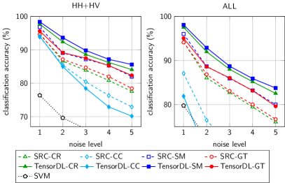
The results of nine different methods are depicted in Figure 7. These methods include SVM (the dotted line), the four SRC-related methods (dashed lines), and their corresponding tensor dictionary learning counterparts (prefixed by TensorDL, solid lines). We can see that except for the CC case, tensor dictionary learning methods outperform their corresponding SRC with gaps widening as the noise level increases. This observation confirms that tensor discriminative dictionary learning methods indeed provide accuracy improvements. Methods with the SM constraint once again emerge the winner in all noise levels, and the best accuracy numbers are observed using the HH+HV combination.

III-F Multiple-relative-look classification accuracy

Figure 8: Multi-relative-look experimental setup (a) and nonzeros locations of sparse tensors in different scenarios (b, c, d).

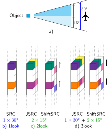
We describe a key real-world scenario where multi-look signals of an object of interest can be obtained. Figure 8a depicts the relative location of a radar carrier, a jet plane in this case, and an object of interest. The plane moves around the object at an angle corresponding to the blue arrow. One sample of object can be captured at this whole range, which can be seen as one of its looks. At the same time, the radar can also capture multiple looks of the object at smaller angles represented by green arrows. By continuing considering even smaller angles, more representatives of the object can be captured. These multiple views can provide complementary information of the object, highly likely resulting in better classification accuracy of the system.

For the training samples, for each object, we generate two sets of signals. Each set contains samples captured after each $15^{\circ}$, and each set has total of 24 views. Both sets start at the same relative angle but the first is captured by an integration angle of $30^{\circ}$, the angle in the second set is $15^{\circ}$. For the test samples, each object is represented by three signals: one by an integration angle of $30^{\circ}$ and two others by an integration angle of $15^{\circ}$, as depicted in Figure 8a. Similar to previous experiments, test samples are captured at random relative angles. Ground samples are also simulated in the same way. Based on three signals captured, we establish three different way of using this information in the classification process:

1. 1look: for each object, we use signals at integration angle of $30^{\circ}$ only. If only one polarization is used, an object of interest can be identified by SRC (and implicitly, SVM). If more than one polarization is involved, one object will be determined by SRC-SM, as this is the best method based on previous experiments (see Figure 8b).

2. 2look: each object is represented by two singles captured at $15^{\circ}$. This multi-look classification problem can be solved by joint SRC (JSRC) [22], or the proposed relative-look SRC (ShiftSRC) (see Figure 8c).

3. 3look: uses all three signals to represent an object. In this case, the relationship between the $30^{\circ}$ signal and the first $15^{\circ}$ signal can be modeled by the SRC-SM, while the relationship between two $15^{\circ}$ signals can be formed by either JSRC or ShiftSRC (see Figure 8d).

Figure 9: Classification accuracy (%) of different methods on multiple-relative-look classification problem.

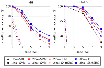
For this experiment, we consider the all-target scenario and two polarization combinations, HH and HH+HV. It is worth noting that for the HH+HV case, there will be four channels in 2look and six channels in 3look. The results of different methods are shown in Figure 9. We can see that SVM still performs well at the lowest noise level (1), but drastically degrades with a little more corruption. On the other hand, SRC-based methods obtain good results even if the noise level is large for the HH+HV combination. Of sparse representation methods, ShiftSRC outperforms the others with the gap becoming larger for highly corrupted signals. Interestingly, ShiftSRC at 2look provides even better results than JSRC does at 3look. These results confirm the advantages of the proposed relative-look sparse representation model.

Figure 10: A VV-polarized SAR image of a minefield collected at Yuma Proving Grounds using the Army Research Laboratory UWB radar.

Figure 11: Visualization of real UWB SAR signals. Top: signals of targets, bottom: signals of confusers.

III-G Overall accuracy on measured UWB SAR data

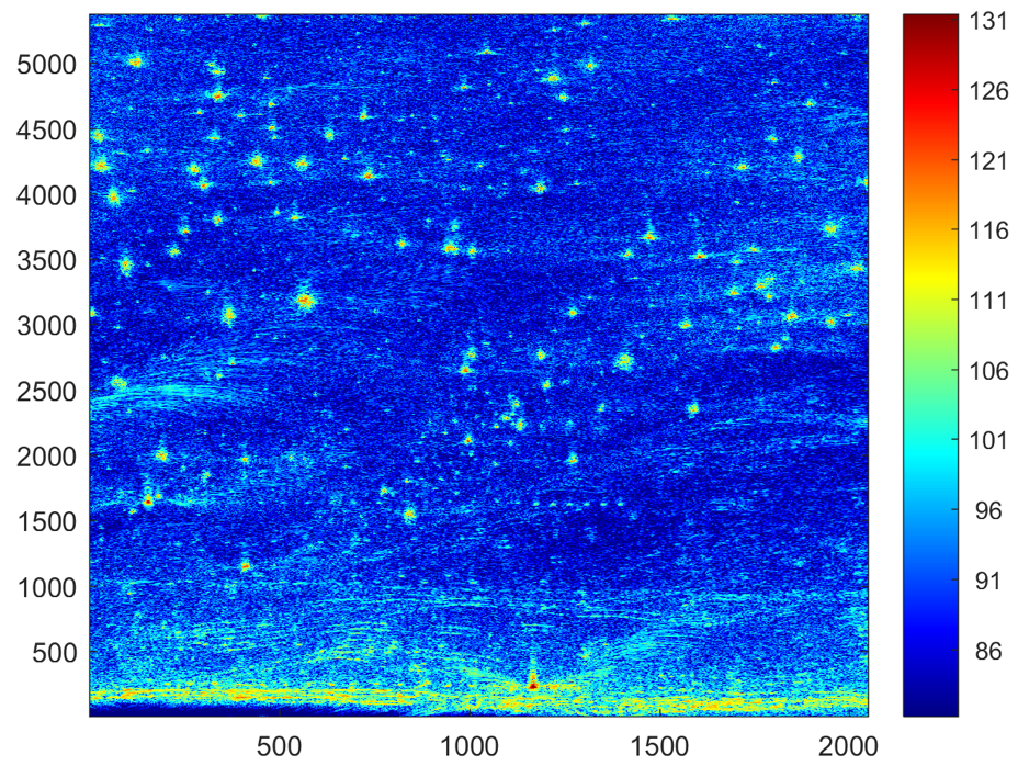
In this section, the results of this technique are illustrated using the data from the ARL UWB low-frequency SAR, which transmits radar signals occupying the frequency spectrum that span approximately from 50 to 1150 MHz [48]. Figure 10 shows a SAR image formed using data collected at Yuma Proving Grounds (YPG) [2]. The scene includes several rows of buried mines surrounded by clutter objects such as bushes, rocks, tire tracks, etc.

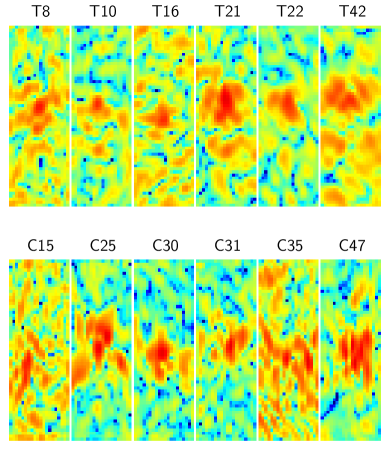
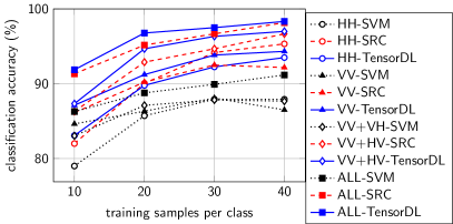
The set contains signals of 50 targets and 50 confusers. Each signal has resolution of $90\times 30$ and already includes noise from the ground. Visualization of six samples in each class are shown in Figure 11. We conduct the all-target experiment and report results of different methods on different polarization combinations in Figure 12. For each combination, three competing methods are considered: SVM, SRC, and TensorDL (both with the SM constraint). Since grounds are fixed in this data set, we report the results based on size of the training set. For each training size $N$ ($N=$10, 20, 30, or 40), we randomly choose $N$ samples from each class for training; the rest $50-N$ samples are considered test samples.

The results are reported in Figure 12 as the average of 10 tests. In general, the tensor dictionary learning performs better than sparse representation in all combinations except for the HH case. SVM also provides good results but is outperformed by other competing methods.

Figure 12: Classification accuracy on real data.

IV Conclusion

We have developed a novel discrimination and classification framework for low-frequency UWB SAR imagery using sparse representation-based methods. The framework is applicable for either single channel or multiple channel (polarizations, multilook) SAR imagery. The techniques are tested and the discrimination/classification performance of targets of interest versus natural and manmade clutter in challenging scenarios is measured using both rigorous electromagnetic simulation data and real data from the ARL UWB radar. The classification results show encouraging potential of tensor sparsity methods, even when the test images are very noisy (buried under extremely rough ground surfaces), targets have small RCSs, and the targets’ responses have very little detailed structures, i.e., targets are small compared to the wavelengths of the radar signals. The SRC-SM technique and its dictionary learning version consistently offers the best results with the combination of co- and cross-pol data, e.g., HH+HV or ALL. In addition, the non-negativity constraints on sparse tensor codes enhance the performance of the systems. Furthermore, we also show the ShiftSRC model is particularly suitable for problems with multiple-relative-look signals.

Tiep Huu Vu received the B.S. degree in Electronics and Telecommunications from Hanoi University of Science and Technology, Vietnam, in 2012. He is currently pursuing the Ph.D. degree with the information Processing and Algorithm Laboratory (iPAL), The Pennsylvania State University, University Park, PA. He did two Research Internships with the Army Research Lab, MD in 2016 and 2017. His research interests are broadly in the areas of statistical learning for signal and image analysis, computer vision and pattern recognition for image classification, segmentation, recovery and retrieval.

Lam H. Nguyen received the B.S.E.E. degree from Virginia Polytechnic Institute, Blacksburg, VA, USA, the M.S.E.E. degree from George Washington University, Washington, DC, USA, and the M.S.C.S. degree from Johns Hopkins University, Baltimore, MD, USA, in 1984, 1991, and 1995, respectively. He started his career with General Electric Company, Portsmouth, VA, in 1984. He joined Harry Diamond Laboratory, Adelphi, MD (and its predecessor Army Research Laboratory) and has worked there from 1986 to the present. Currently, he is a Signal Processing Team Leader with the U.S. Army Research Laboratory, where he has primarily engaged in the research and development of several versions of ultra-wideband (UWB) radar since the early 1990s to the present. These radar systems have been used for proof-of-concept demonstrations in many concealed target detection programs. He has been providing synthetic aperture radar (SAR) signal-processing technical consultations to industry for the developments of many state-of-the-art UWB radars. He has been developing algorithms for SAR signal and image processing. He has authored/coauthored approximately 100 conferences, journals, and technical publications. He has eleven patents in SAR system and signal processing. He has been a member of the SPIE Technical Committee on Radar Sensor Technology since 2009. He was the recipient of the U.S. Army Research and Development Achievement Awards in 2006, 2008, and 2010, the Army Research Laboratory Award for Science in 2010, and the U.S. Army Superior Civilian Performance Award in 2011.

Vishal Monga (SM 2011) is a tenured Associate Professor in the School of Electrical Engineering and Computer Science at the main campus of Pennsylvania State University in University Park, PA. He was with Xerox Research from 2005-2009. His undergraduate work was completed at the Indian Institute of Technology (IIT), Guwahati and his doctoral degree in Electrical Engineering was obtained from the University of Texas, Austin in Aug 2005. Dr. Monga’s research interests are broadly in signal and image processing. His research group at Penn State focuses on convex optimization approaches to image classification, robust signal (time-series) hashing, radar signal processing and computational imaging. He currently serves as an Associate Editor for the IEEE Transactions on Image Processing, IEEE Signal Processing Letters, and the IEEE Transactions on Circuits and Systems for Video Technology. Prof. Monga is a recipient of the US National Science Foundation (NSF) CAREER award, a Monkowski Early Career award from the college of engineering at Penn State and the Joel and Ruth Spira Teaching Excellence Award.

References

- [1] L. H. Nguyen, R. Kapoor, and J. Sichina, “Detection algorithms for ultrawideband foliage-penetration radar,” Proceedings of the SPIE, 3066, pp. 165–176, 1997.
- [2] L. H. Nguyen, K. Kappra, D. Wong, R. Kapoor, and J. Sichina, “Mine field detection algorithm utilizing data from an ultrawideband wide-area surveillance radar,” SPIE International Society of Optical Engineers, 3392, no. 627, 1998.
- [3] L. H. Nguyen, M. Ressler, and J. Sichina, “Sensing through the wall imaging using the Army Research Lab ultra-wideband synchronous impulse reconstruction (UWB SIRE) radar,” Proceedings of SPIE, 6947, no. 69470B, 2008.
- [4] L. Nguyen, R. Kapoor, D. Wong, and J. Sichina, “Ultra-wideband radar target discrimination utilizing an advanced feature set,” SPIE, Algorithms for Synthetic Aperture Radar Imagery V, 1998.
- [5] T. R. Damarla, L. Nguyen, and K. Ranney, “Detection of UXO contaminated land fields using hidden Markov models in the SAR images generated by airborne radar system,” in Proceedings of SPIE, vol. 4374, 2001, p. 61.
- [6] P. Runkle, L. H. Nguyen, J. H. McClellan, and L. Carin, “Multi-aspect target detection for sar imagery using hidden markov models,” IEEE Trans. on Geos. and Remote Sensing, vol. 39, no. 1, pp. 46–55, 2001.
- [7] M. Anabuki, S. Okumura, T. Sato, T. Sakamoto, K. Saho, M. Yoshioka, K. Inoue, T. Fukuda, and H. Sakai, “Ultrawideband radar imaging using adaptive array and doppler separation,” IEEE Transactions on Aerospace and Electronic Systems, vol. 53, no. 1, pp. 190–200, 2017.
- [8] T. Sakamoto, T. Sato, P. Aubry, and A. Yarovoy, “Fast imaging method for security systems using ultrawideband radar,” IEEE Transactions on Aerospace and Electronic Systems, vol. 52, no. 2, pp. 658–670, 2016.
- [9] A. Yamaryo, T. Takatori, S. Kidera, and T. Kirimoto, “Range-point migration-based image expansion method exploiting fully polarimetric data for UWB short-range radar,” IEEE Transactions on Geoscience and Remote Sensing, vol. 56, no. 4, pp. 2170–2182, 2018.
- [10] M. A. Kiasari, S. Y. Na, and J. Y. Kim, “Classification of human postures using ultra-wide band radar based on neural networks,” in IEEE International Conference on IT Convergence and Security (ICITCS), 2014, pp. 1–4.
- [11] J. Bryan, J. Kwon, N. Lee, and Y. Kim, “Application of ultra-wide band radar for classification of human activities,” IET Radar, Sonar & Navigation, vol. 6, no. 3, pp. 172–179, 2012.
- [12] X. Liang, T. Lv, H. Zhang, Y. Gao, and G. Fang, “Through-wall human being detection using UWB impulse radar,” EURASIP Journal on Wireless Communications and Networking, vol. 2018, no. 1, p. 46, 2018.
- [13] D. Wang, L. Chen, D. Piscarreta, and K. W. Tam, “Classification and regression of ultra wide band signals,” in IEEE Chinese Automation Congress (CAC), 2015, pp. 1907–1912.
- [14] J. Wright, A. Yang, A. Ganesh, S. Sastry, and Y. Ma, “Robust face recognition via sparse representation,” IEEE Trans. on Pattern Analysis and Machine Intelligence, vol. 31, no. 2, pp. 210–227, Feb. 2009.
- [15] T. H. Vu, H. S. Mousavi, V. Monga, U. Rao, and G. Rao, “DFDL: Discriminative feature-oriented dictionary learning for histopathological image classification,” IEEE Int. Symposium on Biomedical Imaging, pp. 990–994, 2015.
- [16] U. Srinivas, H. S. Mousavi, C. Jeon, V. Monga, A. Hattel, and B. Jayarao, “SHIRC: A simultaneous sparsity model for histopathological image representation and classification,” IEEE Int. Symposium on Biomedical Imaging, pp. 1118–1121, Apr. 2013.
- [17] T. H. Vu, H. S. Mousavi, V. Monga, U. Rao, and G. Rao, “Histopathological image classification using discriminative feature-oriented dictionary learning,” IEEE Trans. on Medical Imaging, vol. 35, no. 3, pp. 738–751, March, 2016.
- [18] U. Srinivas, H. S. Mousavi, V. Monga, A. Hattel, and B. Jayarao, “Simultaneous sparsity model for histopathological image representation and classification,” IEEE Trans. on Medical Imaging, vol. 33, no. 5, pp. 1163–1179, May 2014.
- [19] X. Sun, N. M. Nasrabadi, and T. D. Tran, “Task-driven dictionary learning for hyperspectral image classification with structured sparsity constraints,” IEEE Trans. on Geos. and Remote Sensing, vol. 53, no. 8, pp. 4457–4471, 2015.
- [20] X. Sun, Q. Qu, N. M. Nasrabadi, and T. D. Tran, “Structured priors for sparse-representation-based hyperspectral image classification,” IEEE Geos. and Remote Sensing Letters, vol. 11, no. 7, pp. 1235–1239, 2014.
- [21] Y. Chen, N. M. Nasrabadi, and T. D. Tran, “Hyperspectral image classification via kernel sparse representation,” IEEE Trans. on Geos. and Remote Sensing, vol. 51, no. 1, pp. 217–231, 2013.
- [22] H. Zhang, N. M. Nasrabadi, Y. Zhang, and T. S. Huang, “Multi-view automatic target recognition using joint sparse representation,” IEEE Trans. on Aerospace and Electronic Systems, vol. 48, no. 3, pp. 2481–2497, 2012.
- [23] X. Mo, V. Monga, R. Bala, and Z. Fan, “Adaptive sparse representations for video anomaly detection,” IEEE Trans. on Circuits and Systems for Video Technology, vol. 24, no. 4, pp. 631–645, 2014.
- [24] T. H. Vu and V. Monga, “Learning a low-rank shared dictionary for object classification,” IEEE Int. Conference on Image Processing, 2016.
- [25] H. S. Mousavi, U. Srinivas, V. Monga, Y. Suo, M. Dao, and T. Tran, “Multi-task image classification via collaborative, hierarchical spike-and-slab priors,” in IEEE Int. Conference on Image Processing, 2014, pp. 4236–4240.
- [26] T. H. Vu and V. Monga, “Fast low-rank shared dictionary learning for image classification,” IEEE Trans. on Image Processing, vol. 26, no. 11, pp. 5160–5175, Nov 2017.
- [27] U. Srinivas, Y. Suo, M. Dao, V. Monga, and T. D. Tran, “Structured sparse priors for image classification,” IEEE Trans. on Image Processing, vol. 24, no. 6, pp. 1763–1776, 2015.
- [28] H. Zhang, Y. Zhang, N. M. Nasrabadi, and T. S. Huang, “Joint-structured-sparsity-based classification for multiple-measurement transient acoustic signals,” IEEE Trans. on Systems, Man, and Cybernetics, Part B: Cybernetics, vol. 42, no. 6, pp. 1586–1598, 2012.
- [29] M. Dao, Y. Suo, S. P. Chin, and T. D. Tran, “Structured sparse representation with low-rank interference,” in IEEE Asilomar Conference on Signals, Systems and Computers, 2014, pp. 106–110.
- [30] M. Dao, N. H. Nguyen, N. M. Nasrabadi, and T. D. Tran, “Collaborative multi-sensor classification via sparsity-based representation,” IEEE Trans. on Signal Processing, vol. 64, no. 9, pp. 2400–2415, 2016.
- [31] H. Van Nguyen, V. M. Patel, N. M. Nasrabadi, and R. Chellappa, “Design of non-linear kernel dictionaries for object recognition,” IEEE Trans. on Image Processing, vol. 22, no. 12, pp. 5123–5135, 2013.
- [32] L. Nguyen and C. Le, “Sparsity driven target discrimination for ultra-wideband (UWB) down-looking Ground penetration radar (GPR),” Tri-Service Radar, 2013.
- [33] J. A. Tropp, A. C. Gilbert, and M. J. Strauss, “Algorithms for simultaneous sparse approximation. part i: Greedy pursuit,” Signal Processing, vol. 86, no. 3, pp. 572–588, 2006.
- [34] A. Beck and M. Teboulle, “A fast iterative shrinkage-thresholding algorithm for linear inverse problems,” SIAM Journal on Imaging Sciences, vol. 2, no. 1, pp. 183–202, 2009.
- [35] T. H. Vu, “DICTOL – A dictionary learning toolbox,” https://github.com/tiepvupsu/DICTOL, 2017, [Online; accessed 15-November-2017].
- [36] T. H. Vu, L. Nguyen, C. Le, and V. Monga, “Tensor sparsity for classifying low-frequency ultra-wideband (UWB) SAR imagery,” 2017, pp. 0557–0562.
- [37] S. Boyd, N. Parikh, E. Chu, B. Peleato, and J. Eckstein, “Distributed optimization and statistical learning via the alternating direction method of multipliers,” Foundations and Trends® in Machine Learning, vol. 3, no. 1, pp. 1–122, 2011.
- [38] “SPArse Modeling Software,” http://spams-devel.gforge.inria.fr/, accessed: 2014-11-05.
- [39] Y. Yu, J. Huang, S. Zhang, C. Restif, X. Huang, and D. Metaxas, “Group sparsity based classification for cervigram segmentation,” IEEE Int. Symposium on Biomedical Imaging, pp. 1425–1429, 2011.
- [40] M. Yang, L. Zhang, X. Feng, and D. Zhang, “Sparse representation based Fisher discrimination dictionary learning for image classification,” Int. Journal of Computer Vision, vol. 109, no. 3, pp. 209–232, 2014.
- [41] I. Ramirez, P. Sprechmann, and G. Sapiro, “Classification and clustering via dictionary learning with structured incoherence and shared features,” in IEEE Int. Conference Computer Vision Pattern Recognition, 2010, pp. 3501–3508.
- [42] T. H. Vu, “Tensor Sparsity Toolbox,” https://github.com/tiepvupsu/tensorsparsity, 2017, [Online; accessed 10-November-2017].
- [43] T. Dogaru, “AFDTD user’s manual,” ARL Technical Report, Adelphi, MD, ARL-TR-5145, March 2010.
- [44] T. Dogaru, L. Nguyen, and C. Le, “Computer models of the human body signature for sensing through the wall radar applications,” ARL, Adelphi, MD, ARL-TR-4290, September 2007.
- [45] D. Liao and T. Dogaru, “Full-wave characterization of rough terrain surface scattering for forward-looking radar applications,” IEEE Trans. on Antenna and Propagation, vol. 60, pp. 3853–3866, August 2012.
- [46] J. McCorkle and L. Nguyen, “Focusing of dispersive targets using synthetic aperture radar,” U.S. Army Research Laboratory, Adelphi, MD, ARL-TR-305, August 1994.
- [47] C.-C. Chang and C.-J. Lin, “LIBSVM: A library for support vector machines,” ACM Trans. on Intelligent Systems and Technology, vol. 2, pp. 27:1–27:27, 2011, software available at http://www.csie.ntu.edu.tw/~cjlin/libsvm.
- [48] M. Ressler, L. Happ, L. Nguyen, T. Ton, and M. Bennett, “The army research laboratory ultra-wide band testbed radars,” in IEEE International Radar Conference, 1995, pp. 686–691.
![[Uncaptioned image]](/html/1810.02812/assets/Vu.jpg) |