Sample Complexity of Sinkhorn Divergences


Aude Genevay                        Lénaic Chizat                        Francis Bach                        Marco Cuturi                        Gabriel Peyré

DMA, ENS Paris                        INRIA                        INRIA and DI, ENS Paris                        Google and CREST ENSAE                        CNRS and DMA, ENS Paris

Abstract

Optimal transport (OT) and maximum mean discrepancies (MMD) are now routinely used in machine learning to compare probability measures. We focus in this paper on Sinkhorn divergences (SDs), a regularized variant of OT distances which can interpolate, depending on the regularization strength ε𝜀\varepsilon, between OT (ε=0𝜀0\varepsilon=0) and MMD (ε=𝜀\varepsilon=\infty). Although the tradeoff induced by that regularization is now well understood computationally (OT, SDs and MMD require respectively O(n3logn)𝑂superscript𝑛3𝑛O(n^{3}\log n), O(n2)𝑂superscript𝑛2O(n^{2}) and n2superscript𝑛2n^{2} operations given a sample size n𝑛n), much less is known in terms of their sample complexity, namely the gap between these quantities, when evaluated using finite samples vs. their respective densities. Indeed, while the sample complexity of OT and MMD stand at two extremes, O(1/n1/d)𝑂1superscript𝑛1𝑑O(1/n^{1/d}) for OT in dimension d𝑑d and O(1/n)𝑂1𝑛O(1/\sqrt{n}) for MMD, that for SDs has only been studied empirically. In this paper, we (i) derive a bound on the approximation error made with SDs when approximating OT as a function of the regularizer ε𝜀\varepsilon, (ii) prove that the optimizers of regularized OT are bounded in a Sobolev (RKHS) ball independent of the two measures and (iii) provide the first sample complexity bound for SDs, obtained,by reformulating SDs as a maximization problem in a RKHS. We thus obtain a scaling in 1/n1𝑛1/\sqrt{n} (as in MMD), with a constant that depends however on ε𝜀\varepsilon, making the bridge between OT and MMD complete.

1 Introduction

Optimal Transport (OT) has emerged in recent years as a powerful tool to compare probability distributions. Indeed, Wasserstein distances can endow the space of probability measures with a rich Riemannian structure (Ambrosio et al., 2006), one that is able to capture meaningful geometric features between measures even when their supports do not overlap. OT has been, however, long neglected in data sciences for two main reasons, which could be loosely described as computational and statistical: computing OT is costly since it requires solving a network flow problem; and suffers from the curse-of-dimensionality, since, as will be made more explicit later in this paper, the Wasserstein distance computed between two samples converges only very slowly to its population counterpart.

Recent years have witnessed significant advances on the computational aspects of OT. A recent wave of works have exploited entropic regularization, both to compare discrete measures with finite support (Cuturi, 2013) or measures that can be sampled from (Genevay et al., 2016). Among the many learning tasks performed with this regularization, one may cite domain adaptation (Courty et al., 2014), text retrieval (Kusner et al., 2015) or multi-label classification (Frogner et al., 2015). The ability of OT to compare probability distributions with disjoint supports (as opposed to the Kullback-Leibler divergence) has also made it popular as a loss function to learn generative models (Arjovsky et al., 2017; Salimans et al., 2018; Beaumont et al., 2002).

At the other end of the spectrum, the maximum mean discrepancy (MMD) (Gretton et al., 2006) is an integral probability metric (Sriperumbudur et al., 2012) on a reproducing kernel Hilbert space (RKHS) of test functions. The MMD is easy to compute, and has also been used in a very wide variety of applications, including for instance the estimation of generative models (Li et al., 2015; MMD-GAN; Li et al., 2017).

OT and MMD differ, however, on a fundamental aspect: their sample complexity. The definition of sample complexity that we choose here is the convergence rate of a given metric between a measure and its empirical counterpart, as a function of the number of samples. This notion is crucial in machine learning, as bad sample complexity implies overfitting and high gradient variance when using these divergences for parameter estimation. In that context, it is well known that the sample complexity of MMD is independent of the dimension, scaling as 1n1𝑛\frac{1}{\sqrt{n}} (Gretton et al., 2006) where n𝑛n is the number of samples. In contrast, it is well known that standard OT suffers from the curse of dimensionality (Dudley, 1969): Its sample complexity is exponential in the dimension of the ambient space. Although it was recently proved that this result can be refined to consider the implicit dimension of data (Weed and Bach, 2017), the sample complexity of OT appears now to be the major bottleneck for the use of OT in high-dimensional machine learning problems.

A remedy to this problem may lie, again, in regularization. Divergences defined through regularized OT, known as Sinkhorn divergences, seem to be indeed less prone to over-fitting. Indeed, a certain amount of regularization seems to improve performance in simple learning tasks (Cuturi, 2013). Additionally, recent papers (Ramdas et al., 2017; Genevay et al., 2018) have pointed out the fact that Sinkhorn divergences are in fact interpolating between OT (when regularization goes to zero) and MMD (when regularization goes to infinity). However, aside from a recent central limit theorem in the case of measures supported on discrete spaces (Bigot et al., 2017), the convergence of empirical Sinkhorn divergences, and more generally their sample complexity, remains an open question.

Contributions.

This paper provides three main contributions, which all exhibit theoretical properties of Sinkhorn divergences. Our first result is a bound on the speed of convergence of regularized OT to standard OT as a function of the regularization parameter, in the case of continuous measures. The second theorem proves that the optimizers of the regularized optimal transport problem lie in a Sobolev ball which is independent of the measures. This allows us to rewrite the Sinkhorn divergence as an expectation maximization problem in a RKHS ball and thus justify the use of kernel-SGD for regularized OT as advocated in (Genevay et al., 2016). As a consequence of this reformulation, we provide as our third contribution a sample complexity result. We focus on how the sample size and the regularization parameter affect the convergence of the empirical Sinkhorn divergence (i.e., computed from samples of two continuous measures) to the continuous Sinkhorn divergence. We show that the Sinkhorn divergence benefits from the same sample complexity as MMD, scaling in 1n1𝑛\frac{1}{\sqrt{n}} but with a constant that depends on the inverse of the regularization parameter. Thus sample complexity worsens when getting closer to standard OT, and there is therefore a tradeoff between a good approximation of OT (small regularization parameter) and fast convergence in terms of sample size (larger regularization parameter). We conclude this paper with a few numerical experiments to asses the dependence of the sample complexity on ε𝜀\varepsilon and d𝑑d in very simple cases.

Notations.

We consider 𝒳𝒳\mathcal{X} and 𝒴𝒴\mathcal{Y} two bounded subsets of dsuperscript𝑑\mathbb{R}^{d} and we denote by |𝒳|𝒳|\mathcal{X}| and |𝒴|𝒴|\mathcal{Y}| their respective diameter sup{||xx|||x,x𝒳(resp.𝒴)}\sup\{|\!|x-x^{\prime}|\!||x,x^{\prime}\in\mathcal{X}(resp.\mathcal{Y})\}. The space of positive Radon measures of mass 1 on 𝒳𝒳\mathcal{X} is denoted +1(𝒳)superscriptsubscript1𝒳\mathcal{M}_{+}^{1}(\mathcal{X}) and we use upper cases X,Y𝑋𝑌X,Y to denote random variables in these spaces. We use the notation φ=O(1+xk)𝜑𝑂1superscript𝑥𝑘\varphi=O(1+x^{k}) to say that φ𝜑\varphi\in\mathbb{R} is bounded by a polynomial of order k𝑘k in x𝑥x with positive coefficients.

2 Reminders on Sinkhorn Divergences

We consider two probability measures α+1(𝒳)𝛼superscriptsubscript1𝒳\alpha\in\mathcal{M}_{+}^{1}(\mathcal{X}) and β𝛽\beta on +1(𝒴)superscriptsubscript1𝒴\mathcal{M}_{+}^{1}(\mathcal{Y}). The Kantorovich formulation (1942) of optimal transport between α𝛼\alpha and β𝛽\beta is defined by

W(α,β)=def.minπΠ(α,β)𝒳×𝒴c(x,y)dπ(x,y),superscriptdef.𝑊𝛼𝛽subscript𝜋Π𝛼𝛽subscript𝒳𝒴𝑐𝑥𝑦differential-d𝜋𝑥𝑦W(\alpha,\beta)\stackrel{{\scriptstyle\mbox{def.}}}{{=}}\min_{\pi\in\Pi(\alpha,\beta)}\int_{\mathcal{X}\times\mathcal{Y}}c(x,y)\mathrm{d}\pi(x,y), (𝒫𝒫\mathcal{P})

where the feasible set is composed of probability distributions over the product space 𝒳×𝒴𝒳𝒴\mathcal{X}\times\mathcal{Y} with fixed marginals α,β𝛼𝛽\alpha,\beta:

Π(α,β)=def.{π+1(𝒳×𝒴);P1π=α,P2π=β},superscriptdef.Π𝛼𝛽formulae-sequence𝜋superscriptsubscript1𝒳𝒴formulae-sequencesubscript𝑃1𝜋𝛼subscript𝑃2𝜋𝛽\Pi(\alpha,\beta)\stackrel{{\scriptstyle\mbox{def.}}}{{=}}\left\{\pi\in\mathcal{M}_{+}^{1}(\mathcal{X}\times\mathcal{Y})\;;\;P_{1\sharp}\pi=\alpha,P_{2\sharp}\pi=\beta\right\},

where P1πsubscript𝑃1𝜋P_{1\sharp}\pi (resp. P2πsubscript𝑃2𝜋P_{2\sharp}\pi) is the marginal distribution of π𝜋\pi for the first (resp. second) variable, using the projection maps P1(x,y)=x;P2(x,y)=yformulae-sequencesubscript𝑃1𝑥𝑦𝑥subscript𝑃2𝑥𝑦𝑦P_{1}(x,y)=x;P_{2}(x,y)=y along with the push-forward operator .

The cost function c𝑐c represents the cost to move a unit of mass from x𝑥x to y𝑦y. Through this paper, we will assume this function to be 𝒞superscript𝒞\mathcal{C}^{\infty} (more specifically, we need it to be 𝒞d2+1superscript𝒞𝑑21\mathcal{C}^{\frac{d}{2}+1}). When 𝒳=𝒴𝒳𝒴\mathcal{X}=\mathcal{Y} is endowed with a distance d𝒳subscript𝑑𝒳d_{\mathcal{X}}, choosing c(x,y)=d𝒳(x,y)p𝑐𝑥𝑦subscript𝑑𝒳superscript𝑥𝑦𝑝c(x,y)=d_{\mathcal{X}}(x,y)^{p} where p1𝑝1p\geqslant 1 yields the p𝑝p-Wasserstein distance between probability measures.

We introduce regularized optimal transport, which consists in adding an entropic regularization to the optimal transport problem, as proposed in (Cuturi, 2013). Here we use the relative entropy of the transport plan with respect to the product measure αβtensor-product𝛼𝛽\alpha\otimes\beta following (Genevay et al., 2016):

Wε(α,β)=def.minπΠ(α,β)𝒳×𝒴superscriptdef.subscript𝑊𝜀𝛼𝛽subscript𝜋Π𝛼𝛽subscript𝒳𝒴\displaystyle W_{\varepsilon}(\alpha,\beta)\stackrel{{\scriptstyle\mbox{def.}}}{{=}}\!\min_{\pi\in\Pi(\alpha,\beta)}\int_{\mathcal{X}\times\mathcal{Y}}\!\!\! c(x,y)dπ(x,y)𝑐𝑥𝑦d𝜋𝑥𝑦\displaystyle c(x,y)\mathrm{d}\pi(x,y)
+εH(παβ),𝜀𝐻conditional𝜋tensor-product𝛼𝛽\displaystyle+\varepsilon H(\pi\mid\alpha\otimes\beta), (𝒫εsubscript𝒫𝜀\mathcal{P}_{\varepsilon})

where

H(παβ)=def.𝒳×𝒴log(dπ(x,y)dα(x)dβ(y))dπ(x,y).superscriptdef.𝐻conditional𝜋tensor-product𝛼𝛽subscript𝒳𝒴d𝜋𝑥𝑦d𝛼𝑥d𝛽𝑦differential-d𝜋𝑥𝑦H(\pi\mid\alpha\otimes\beta)\stackrel{{\scriptstyle\mbox{def.}}}{{=}}\int_{\mathcal{X}\times\mathcal{Y}}\log\left(\frac{\mathrm{d}\pi(x,y)}{\mathrm{d}\alpha(x)\mathrm{d}\beta(y)}\right)\mathrm{d}\pi(x,y). (1)

Choosing the relative entropy as a regularizer allows to express the dual formulation of regularized OT as the maximization of an expectation problem, as shown in (Genevay et al., 2016)

Wε(α,β)=subscript𝑊𝜀𝛼𝛽absent\displaystyle W_{\varepsilon}(\alpha,\beta)= maxu𝒞(𝒳),v𝒞(𝒴)𝒳u(x)dα(x)+𝒴v(y)dβ(y)subscriptformulae-sequence𝑢𝒞𝒳𝑣𝒞𝒴subscript𝒳𝑢𝑥differential-d𝛼𝑥subscript𝒴𝑣𝑦differential-d𝛽𝑦\displaystyle\max_{u\in\mathcal{C}(\mathcal{X}),v\in\mathcal{C}(\mathcal{Y})}\int_{\mathcal{X}}u(x)\mathrm{d}\alpha(x)+\int_{\mathcal{Y}}v(y)\mathrm{d}\beta(y)
ε𝒳×𝒴eu(x)+v(y)c(x,y)εdα(x)dβ(y)+ε𝜀subscript𝒳𝒴superscript𝑒𝑢𝑥𝑣𝑦𝑐𝑥𝑦𝜀differential-d𝛼𝑥differential-d𝛽𝑦𝜀\displaystyle-\varepsilon\int_{\mathcal{X}\times\mathcal{Y}}e^{\frac{u(x)+v(y)-c(x,y)}{\varepsilon}}\mathrm{d}\alpha(x)\mathrm{d}\beta(y)+\varepsilon
=\displaystyle= maxu𝒞(X),v𝒞(Y)𝔼αβ[fεXY(u,v)]+εsubscriptformulae-sequence𝑢𝒞𝑋𝑣𝒞𝑌subscript𝔼tensor-product𝛼𝛽delimited-[]superscriptsubscript𝑓𝜀𝑋𝑌𝑢𝑣𝜀\displaystyle\max_{u\in\mathcal{C}(X),v\in\mathcal{C}(Y)}\mathbb{E}_{\alpha\otimes\beta}\left[f_{\varepsilon}^{XY}(u,v)\right]+\varepsilon

where fεxy(u,v)=u(x)+v(y)εeu(x)+v(y)c(x,y)ε.superscriptsubscript𝑓𝜀𝑥𝑦𝑢𝑣𝑢𝑥𝑣𝑦𝜀superscript𝑒𝑢𝑥𝑣𝑦𝑐𝑥𝑦𝜀f_{\varepsilon}^{xy}(u,v)=u(x)+v(y)-\varepsilon e^{\frac{u(x)+v(y)-c(x,y)}{\varepsilon}}. This reformulation as the maximum of an expectation will prove crucial to obtain sample complexity results. The existence of optimal dual potentials (u,v)𝑢𝑣(u,v) is proved in the appendix. They are unique αlimit-from𝛼\alpha- and βlimit-from𝛽\beta-a.e. up to an additive constant.

To correct for the fact that Wε(α,α)0subscript𝑊𝜀𝛼𝛼0W_{\varepsilon}(\alpha,\alpha)\neq 0, (Genevay et al., 2018) propose Sinkhorn divergences, a natural normalization of that quantity defined as

W¯ε(α,β)=Wε(α,β)12(Wε(α,α)+Wε(β,β)).subscript¯𝑊𝜀𝛼𝛽subscript𝑊𝜀𝛼𝛽12subscript𝑊𝜀𝛼𝛼subscript𝑊𝜀𝛽𝛽\bar{W}_{\varepsilon}(\alpha,\beta)=W_{\varepsilon}(\alpha,\beta)-\frac{1}{2}(W_{\varepsilon}(\alpha,\alpha)+W_{\varepsilon}(\beta,\beta)). (2)

This normalization ensures that W¯ε(α,α)=0subscript¯𝑊𝜀𝛼𝛼0\bar{W}_{\varepsilon}(\alpha,\alpha)=0, but also has a noticeable asymptotic behavior as mentioned in (Genevay et al., 2018). Indeed, when ε0𝜀0\varepsilon\rightarrow 0 one recovers the original (unregularized) OT problem, while choosing ε+𝜀\varepsilon\rightarrow+\infty yields the maximum mean discrepancy associated to the kernel k=c/2𝑘𝑐2k=-c/2, where MMD is defined by:

MMDk(α,β)=𝔼αα[k(X,X)]𝑀𝑀subscript𝐷𝑘𝛼𝛽subscript𝔼tensor-product𝛼𝛼delimited-[]𝑘𝑋superscript𝑋\displaystyle MMD_{k}(\alpha,\beta)=\mathbb{E}_{\alpha\otimes\alpha}[k(X,X^{\prime})] +𝔼ββ[k(Y,Y)]subscript𝔼tensor-product𝛽𝛽delimited-[]𝑘𝑌superscript𝑌\displaystyle+\mathbb{E}_{\beta\otimes\beta}[k(Y,Y^{\prime})]
2𝔼αβ[k(X,Y)].2subscript𝔼tensor-product𝛼𝛽delimited-[]𝑘𝑋𝑌\displaystyle-2\mathbb{E}_{\alpha\otimes\beta}[k(X,Y)].

In the context of this paper, we study in detail the sample complexity of Wε(α,β)subscript𝑊𝜀𝛼𝛽W_{\varepsilon}(\alpha,\beta), knowing that these results can be extended to W¯ε(α,β)subscript¯𝑊𝜀𝛼𝛽\bar{W}_{\varepsilon}(\alpha,\beta).

3 Approximating Optimal Transport with Sinkhorn Divergences

In the present section, we are interested in bounding the error made when approximating W(α,β)𝑊𝛼𝛽W(\alpha,\beta) with Wε(α,β)subscript𝑊𝜀𝛼𝛽W_{\varepsilon}(\alpha,\beta).

Theorem 1.

Let α𝛼\alpha and β𝛽\beta be probability measures on 𝒳𝒳\mathcal{X} and 𝒴𝒴\mathcal{Y} subsets of dsuperscript𝑑\mathbb{R}^{d} such that |𝒳|=|𝒴|D𝒳𝒴𝐷|\mathcal{X}|=|\mathcal{Y}|\leqslant D and assume that c𝑐c is L𝐿L-Lipschitz w.r.t. x𝑥x and y𝑦y. It holds

0Wε(α,β)W(α,β)0subscript𝑊𝜀𝛼𝛽𝑊𝛼𝛽\displaystyle 0\leqslant W_{\varepsilon}(\alpha,\beta)-W(\alpha,\beta) 2εdlog(e2LDdε)absent2𝜀𝑑superscript𝑒2𝐿𝐷𝑑𝜀\displaystyle\leqslant 2\varepsilon d\log\left(\frac{e^{2}\cdot L\cdot D}{\sqrt{d}\cdot\varepsilon}\right) (3)
ε02εdlog(1/ε).subscriptsimilar-to𝜀0absent2𝜀𝑑1𝜀\displaystyle\sim_{\varepsilon\to 0}2\varepsilon d\log(1/\varepsilon). (4)
Proof.

For a probability measure π𝜋\pi on 𝒳×𝒴𝒳𝒴\mathcal{X}\times\mathcal{Y}, we denote by C(π)=cdπ𝐶𝜋𝑐differential-d𝜋C(\pi)=\int c\,\mathrm{d}\pi the associated transport cost and by H(π)𝐻𝜋H(\pi) its relative entropy with respect to the product measure αβtensor-product𝛼𝛽\alpha\otimes\beta as defined in (1). Choosing π0subscript𝜋0\pi_{0} a minimizer of minπΠ(α,β)C(π)subscript𝜋Π𝛼𝛽𝐶𝜋\min_{\pi\in\Pi(\alpha,\beta)}C(\pi), we will build our upper bounds using a family of transport plans with finite entropy that approximate π0subscript𝜋0\pi_{0}. The simplest approach consists in considering block approximation. In contrast to the work of Carlier et al. (2017), who also considered this technique, our focus here is on quantitative bounds.

Definition 1 (Block approximation).

For a resolution Δ>0Δ0\Delta>0, we consider the block partition of dsuperscript𝑑\mathbb{R}^{d} in hypercubes of side ΔΔ\Delta defined as

{QkΔ=[k1Δ,(k1+1)Δ[×[kdΔ,(kd+1)Δ[;\displaystyle\{Q^{\Delta}_{k}={[k_{1}\cdot\Delta,(k_{1}+1)\cdot\Delta[}\times\dots[k_{d}\cdot\Delta,(k_{d}+1)\cdot\Delta[\;;
k=(k1,,kd)d}.\displaystyle k=(k_{1},\dots,k_{d})\in\mathbb{Z}^{d}\}.

To simplify notations, we introduce QijΔ=def.QiΔ×QjΔsuperscriptdef.subscriptsuperscript𝑄Δ𝑖𝑗subscriptsuperscript𝑄Δ𝑖subscriptsuperscript𝑄Δ𝑗Q^{\Delta}_{ij}\stackrel{{\scriptstyle\mbox{def.}}}{{=}}Q^{\Delta}_{i}\times Q^{\Delta}_{j}, 𝛂iΔ=def.α(QiΔ)superscriptdef.superscriptsubscript𝛂𝑖Δ𝛼superscriptsubscript𝑄𝑖Δ\boldsymbol{\alpha}_{i}^{\Delta}\stackrel{{\scriptstyle\mbox{def.}}}{{=}}\alpha(Q_{i}^{\Delta}), 𝛃jΔ=def.β(QjΔ)superscriptdef.superscriptsubscript𝛃𝑗Δ𝛽superscriptsubscript𝑄𝑗Δ\boldsymbol{\beta}_{j}^{\Delta}\stackrel{{\scriptstyle\mbox{def.}}}{{=}}\beta(Q_{j}^{\Delta}). The block approximation of π0subscript𝜋0\pi_{0} of resolution ΔΔ\Delta is the measure πΔΠ(α,β)superscript𝜋ΔΠ𝛼𝛽\pi^{\Delta}\in\Pi(\alpha,\beta) characterized by

πΔ|QijΔ=π0(QijΔ)𝜶iΔ𝜷jΔ(α|QiΔβ|QjΔ)evaluated-atsuperscript𝜋Δsubscriptsuperscript𝑄Δ𝑖𝑗subscript𝜋0subscriptsuperscript𝑄Δ𝑖𝑗superscriptsubscript𝜶𝑖Δsuperscriptsubscript𝜷𝑗Δevaluated-attensor-productevaluated-at𝛼subscriptsuperscript𝑄Δ𝑖𝛽subscriptsuperscript𝑄Δ𝑗\pi^{\Delta}|_{Q^{\Delta}_{ij}}=\frac{\pi_{0}(Q^{\Delta}_{ij})}{\boldsymbol{\alpha}_{i}^{\Delta}\cdot\boldsymbol{\beta}_{j}^{\Delta}}(\alpha|_{Q^{\Delta}_{i}}\otimes\beta|_{Q^{\Delta}_{j}})

for all (i,j)(d)2𝑖𝑗superscriptsuperscript𝑑2(i,j)\in(\mathbb{Z}^{d})^{2}, with the convention 0/0=00000/0=0.

πΔsuperscript𝜋Δ\pi^{\Delta} is nonnegative by construction. Observe also that for any Borel set Bd𝐵superscript𝑑B\subset\mathbb{R}^{d}, one has

πΔ(B×d)superscript𝜋Δ𝐵superscript𝑑\displaystyle\pi^{\Delta}(B\times\mathbb{R}^{d}) =(i,j)(d)2π0(QijΔ)𝜶iΔ𝜷jΔα(BQiΔ)𝜷jΔabsentsubscript𝑖𝑗superscriptsuperscript𝑑2subscript𝜋0superscriptsubscript𝑄𝑖𝑗Δsuperscriptsubscript𝜶𝑖Δsuperscriptsubscript𝜷𝑗Δ𝛼𝐵subscriptsuperscript𝑄Δ𝑖superscriptsubscript𝜷𝑗Δ\displaystyle=\sum_{(i,j)\in(\mathbb{Z}^{d})^{2}}\frac{\pi_{0}(Q_{ij}^{\Delta})}{\boldsymbol{\alpha}_{i}^{\Delta}\cdot\boldsymbol{\beta}_{j}^{\Delta}}\cdot\alpha(B\cap Q^{\Delta}_{i})\cdot\boldsymbol{\beta}_{j}^{\Delta}
=idα(BQiΔ)=α(B),absentsubscript𝑖superscript𝑑𝛼𝐵subscriptsuperscript𝑄Δ𝑖𝛼𝐵\displaystyle=\sum_{i\in\mathbb{Z}^{d}}\alpha(B\cap Q^{\Delta}_{i})=\alpha(B),

which proves, using the symmetric result in β𝛽\beta, that πΔsuperscript𝜋Δ\pi^{\Delta} belongs to Π(α,β)Π𝛼𝛽\Pi(\alpha,\beta). As a consequence, for any ε>0𝜀0\varepsilon>0 one has Wε(α,β)C(πΔ)+εH(πΔ)subscript𝑊𝜀𝛼𝛽𝐶superscript𝜋Δ𝜀𝐻superscript𝜋ΔW_{\varepsilon}(\alpha,\beta)\leqslant C(\pi^{\Delta})+\varepsilon H(\pi^{\Delta}). Recalling also that the relative entropy H𝐻H is nonnegative over the set of probability measures, we have the bound

0Wε(α,β)W(α,β)(C(πΔ)C(π0))+εH(πΔ).0subscript𝑊𝜀𝛼𝛽𝑊𝛼𝛽𝐶superscript𝜋Δ𝐶subscript𝜋0𝜀𝐻superscript𝜋Δ0\leqslant W_{\varepsilon}(\alpha,\beta)-W(\alpha,\beta)\leqslant(C(\pi^{\Delta})-C(\pi_{0}))+\varepsilon H(\pi^{\Delta}).

We can now bound the terms in the right-hand side, and choose a value for ΔΔ\Delta that minimizes these bounds.

The bound on C(πΔ)C(π0)𝐶superscript𝜋Δ𝐶subscript𝜋0C(\pi^{\Delta})-C(\pi_{0}) relies on the Lipschitz regularity of the cost function. Using the fact that πΔ(QijΔ)=π0(QijΔ)superscript𝜋Δsubscriptsuperscript𝑄Δ𝑖𝑗subscript𝜋0subscriptsuperscript𝑄Δ𝑖𝑗\pi^{\Delta}(Q^{\Delta}_{ij})=\pi_{0}(Q^{\Delta}_{ij}) for all i,j𝑖𝑗i,j, it holds

C(πΔ)C(π0)𝐶superscript𝜋Δ𝐶subscript𝜋0\displaystyle C(\pi^{\Delta})-C(\pi_{0}) =(i,j)(d)2π0(QijΔ)(supx,yQijΔc(x,y)\displaystyle=\sum_{(i,j)\in(\mathbb{Z}^{d})^{2}}\pi_{0}(Q^{\Delta}_{ij})\Big{(}\sup_{x,y\in Q^{\Delta}_{ij}}c(x,y)
infx,yQijΔc(x,y))\displaystyle\phantom{\sum_{(i,j)\in(\mathbb{Z}^{d})^{2}}\pi_{0}(Q^{\Delta}_{ij})\Big{(}}-\inf_{x,y\in Q^{\Delta}_{ij}}c(x,y)\Big{)}
2LΔd,absent2𝐿Δ𝑑\displaystyle\leqslant 2L\Delta\sqrt{d},

where L𝐿L is the Lipschitz constant of the cost (separately in x𝑥x and y𝑦y) and ΔdΔ𝑑\Delta\sqrt{d} is the diameter of each set QiΔsubscriptsuperscript𝑄Δ𝑖Q^{\Delta}_{i}.

As for the bound on H(πΔ)𝐻superscript𝜋ΔH(\pi^{\Delta}), using the fact that π0(QijΔ)1subscript𝜋0subscriptsuperscript𝑄Δ𝑖𝑗1\pi_{0}(Q^{\Delta}_{ij})\leqslant 1 we get

H(πΔ)𝐻superscript𝜋Δ\displaystyle H(\pi^{\Delta}) =(i,j)(d)2log(π0(QijΔ)𝜶iΔ𝜷jΔ)π0(QijΔ)absentsubscript𝑖𝑗superscriptsuperscript𝑑2subscript𝜋0subscriptsuperscript𝑄Δ𝑖𝑗superscriptsubscript𝜶𝑖Δsuperscriptsubscript𝜷𝑗Δsubscript𝜋0subscriptsuperscript𝑄Δ𝑖𝑗\displaystyle=\!\!\sum_{(i,j)\in(\mathbb{Z}^{d})^{2}}\!\log\left(\frac{\pi_{0}(Q^{\Delta}_{ij})}{\boldsymbol{\alpha}_{i}^{\Delta}\cdot\boldsymbol{\beta}_{j}^{\Delta}}\right)\pi_{0}(Q^{\Delta}_{ij})
(i,j)(d)2(log(1/𝜶iΔ)+log(1/𝜷jΔ))π0(QijΔ)absentsubscript𝑖𝑗superscriptsuperscript𝑑21superscriptsubscript𝜶𝑖Δ1superscriptsubscript𝜷𝑗Δsubscript𝜋0subscriptsuperscript𝑄Δ𝑖𝑗\displaystyle\leqslant\sum_{(i,j)\in(\mathbb{Z}^{d})^{2}}\left(\log(1/\boldsymbol{\alpha}_{i}^{\Delta})+\log(1/\boldsymbol{\beta}_{j}^{\Delta})\right)\pi_{0}(Q^{\Delta}_{ij})
=HΔ(α)HΔ(β),absentsuperscript𝐻Δ𝛼superscript𝐻Δ𝛽\displaystyle=-H^{\Delta}(\alpha)-H^{\Delta}(\beta),

where we have defined HΔ(α)=id𝜶iΔlog(𝜶iΔ)superscript𝐻Δ𝛼subscript𝑖superscript𝑑superscriptsubscript𝜶𝑖Δsuperscriptsubscript𝜶𝑖ΔH^{\Delta}(\alpha)=\sum_{i\in\mathbb{Z}^{d}}\boldsymbol{\alpha}_{i}^{\Delta}\log(\boldsymbol{\alpha}_{i}^{\Delta}) and similarly for β𝛽\beta. Note that in case α𝛼\alpha is a discrete measure with finite support, HΔ(α)superscript𝐻Δ𝛼H^{\Delta}(\alpha) is equal to (minus) the discrete entropy of α𝛼\alpha as long as ΔΔ\Delta is smaller than the minimum separation between atoms of α𝛼\alpha. However, if α𝛼\alpha is not discrete then HΔ(α)superscript𝐻Δ𝛼H^{\Delta}(\alpha) blows up to -\infty as ΔΔ\Delta goes to 00 and we need to control how fast it does so. Considering αΔsuperscript𝛼Δ\alpha^{\Delta} the block approximation of α𝛼\alpha with constant density 𝜶iΔ/Δdsuperscriptsubscript𝜶𝑖ΔsuperscriptΔ𝑑\boldsymbol{\alpha}_{i}^{\Delta}/\Delta^{d} on each block QiΔsubscriptsuperscript𝑄Δ𝑖Q^{\Delta}_{i} and (minus) its differential entropy Hd(αΔ)=dαΔ(x)logαΔ(x)𝑑xsubscript𝐻superscript𝑑superscript𝛼Δsubscriptsuperscript𝑑superscript𝛼Δ𝑥superscript𝛼Δ𝑥differential-d𝑥H_{\mathcal{L}^{d}}(\alpha^{\Delta})=\int_{\mathbb{R}^{d}}\alpha^{\Delta}(x)\log\alpha^{\Delta}(x)dx, it holds HΔ(α)=Hd(αΔ)dlog(1/Δ)superscript𝐻Δ𝛼subscript𝐻superscript𝑑superscript𝛼Δ𝑑1ΔH^{\Delta}(\alpha)=H_{\mathcal{L}^{d}}(\alpha^{\Delta})-d\cdot\log(1/\Delta). Moreover, using the convexity of Hdsubscript𝐻superscript𝑑H_{\mathcal{L}^{d}}, this can be compared with the differential entropy of the uniform probability on a hypercube containing 𝒳𝒳\mathcal{X} of size 2D2𝐷2D. Thus it holds Hd(αΔ)dlog(2D)subscript𝐻superscript𝑑superscript𝛼Δ𝑑2𝐷H_{\mathcal{L}^{d}}(\alpha^{\Delta})\geqslant-d\log(2D) and thus HΔ(α)dlog(2D/Δ)superscript𝐻Δ𝛼𝑑2𝐷ΔH^{\Delta}(\alpha)\geqslant-d\cdot\log(2D/\Delta).

Summing up, we have for all Δ>0Δ0\Delta>0

Wε(α,β)W(α,β)2LΔd+2εdlog(2D/Δ).subscript𝑊𝜀𝛼𝛽𝑊𝛼𝛽2𝐿Δ𝑑2𝜀𝑑2𝐷ΔW_{\varepsilon}(\alpha,\beta)-W(\alpha,\beta)\leqslant 2L\Delta\sqrt{d}+2\varepsilon d\cdot\log(2D/\Delta).

The above bound is convex in ΔΔ\Delta, minimized with Δ=2dε/LΔ2𝑑𝜀𝐿\Delta=2\sqrt{d}\cdot\varepsilon/L. This yields

Wε(α,β)W(α,β)4εd+2εdlog(LDdε).subscript𝑊𝜀𝛼𝛽𝑊𝛼𝛽4𝜀𝑑2𝜀𝑑𝐿𝐷𝑑𝜀W_{\varepsilon}(\alpha,\beta)-W(\alpha,\beta)\leqslant 4\varepsilon d+2\varepsilon d\log\left(\frac{L\cdot D}{\sqrt{d}\cdot\varepsilon}\right).\qed

4 Properties of Sinkhorn Potentials

We prove in this section that Sinkhorn potentials are bounded in the Sobolev space 𝐇s(d)superscript𝐇𝑠superscript𝑑\mathbf{H}^{s}(\mathbb{R}^{d}) regardless of the marginals α𝛼\alpha and β𝛽\beta. For s>d2𝑠𝑑2s>\frac{d}{2}, 𝐇s(d)superscript𝐇𝑠superscript𝑑\mathbf{H}^{s}(\mathbb{R}^{d}) is a reproducing kernel Hilbert space (RKHS): This property will be crucial to establish sample complexity results later on, using standard tools from RKHS theory.

Definition 2.

The Sobolev space 𝐇s(𝒳)superscript𝐇𝑠𝒳\mathbf{H}^{s}(\mathcal{X}), for s𝑠superscripts\in\mathbb{N}^{*}, is the space of functions φ:𝒳d:𝜑𝒳superscript𝑑\varphi:\mathcal{X}\subseteq\mathbb{R}^{d}\rightarrow\mathbb{R} such that for every multi-index k𝑘k with |k|s𝑘𝑠|k|\leqslant s the mixed partial derivative φ(k)superscript𝜑𝑘\varphi^{(k)} exists and belongs to L2(𝒳)superscript𝐿2𝒳L^{2}(\mathcal{X}). It is endowed with the following inner-product

φ,ψ𝐇s(𝒳)=|k|s𝒳φ(k)(x)ψ(k)(x)dx.subscript𝜑𝜓superscript𝐇𝑠𝒳subscript𝑘𝑠subscript𝒳superscript𝜑𝑘𝑥superscript𝜓𝑘𝑥differential-d𝑥\langle\varphi,\psi\rangle_{\mathbf{H}^{s}(\mathcal{X})}=\sum_{|k|\leqslant s}\int_{\mathcal{X}}\varphi^{(k)}(x)\psi^{(k)}(x)\mathrm{d}x. (5)
Theorem 2.

When 𝒳𝒳\mathcal{X} and 𝒴𝒴\mathcal{Y} are two compact sets of dsuperscript𝑑\mathbb{R}^{d} and the cost c𝑐c is 𝒞superscript𝒞\mathcal{C}^{\infty}, then the Sinkhorn potentials (u,v)𝑢𝑣(u,v) are uniformly bounded in the Sobolev space 𝐇s(d)superscript𝐇𝑠superscript𝑑\mathbf{H}^{s}(\mathbb{R}^{d}) and their norms satisfy

u𝐇s=O(1+1εs1)andv𝐇s=O(1+1εs1),subscriptnorm𝑢superscript𝐇𝑠𝑂11superscript𝜀𝑠1andsubscriptnorm𝑣superscript𝐇𝑠𝑂11superscript𝜀𝑠1|\!|u|\!|_{\mathbf{H}^{s}}=O\left(1+\frac{1}{\varepsilon^{s-1}}\right)\;\text{and}\;|\!|v|\!|_{\mathbf{H}^{s}}=O\left(1+\frac{1}{\varepsilon^{s-1}}\right),

with constants that only depend on |𝒳|𝒳|\mathcal{X}| (or |𝒴|𝒴|\mathcal{Y}| for v𝑣v),d𝑑d, and c(k)subscriptnormsuperscript𝑐𝑘\left\|c^{(k)}\right\|_{\infty} for k=0,,s𝑘0𝑠k=0,\dots,s. In particular, we get the following asymptotic behavior in ε𝜀\varepsilon: u𝐇s=O(1)subscriptnorm𝑢superscript𝐇𝑠𝑂1|\!|u|\!|_{\mathbf{H}^{s}}=O(1) as ε+𝜀\varepsilon\rightarrow+\infty and u𝐇s=O(1εs1)subscriptnorm𝑢superscript𝐇𝑠𝑂1superscript𝜀𝑠1|\!|u|\!|_{\mathbf{H}^{s}}=O(\frac{1}{\varepsilon^{s-1}}) as ε0𝜀0\varepsilon\rightarrow 0.

To prove this theorem, we first need to state some regularity properties of the Sinkhorn potentials.

Proposition 1.

If 𝒳𝒳\mathcal{X} and 𝒴𝒴\mathcal{Y} are two compact sets of dsuperscript𝑑\mathbb{R}^{d} and the cost c𝑐c is 𝒞superscript𝒞\mathcal{C}^{\infty}, then

  • u(x)[minyv(y)c(x,y),maxyv(y)c(x,y)]𝑢𝑥subscript𝑦𝑣𝑦𝑐𝑥𝑦subscript𝑦𝑣𝑦𝑐𝑥𝑦u(x)\in[\min_{y}v(y)-c(x,y),\max_{y}v(y)-c(x,y)] for all x𝒳𝑥𝒳x\in\mathcal{X}

  • u𝑢u is L-Lipschitz, where L is the Lipschitz constant of c𝑐c

  • u𝒞(𝒳)𝑢superscript𝒞𝒳u\in\mathcal{C}^{\infty}(\mathcal{X}) and u(k)=O(1+1εk1)subscriptnormsuperscript𝑢𝑘𝑂11superscript𝜀𝑘1\left\|u^{(k)}\right\|_{\infty}=O(1+\frac{1}{\varepsilon^{k-1}})

and the same results also stand for v𝑣v (inverting u𝑢u and v𝑣v in the first item, and replacing 𝒳𝒳\mathcal{X} by 𝒴𝒴\mathcal{Y}).

Proof.

The proofs of all three claims exploit the optimality condition of the dual problem:

exp(u(x)ε)=exp(v(y)c(x,y)ε)β(y)dy.𝑢𝑥𝜀𝑣𝑦𝑐𝑥𝑦𝜀𝛽𝑦differential-d𝑦\!\!\!\exp\left(\frac{-u(x)}{\varepsilon}\right)=\int\exp\left(\frac{v(y)-c(x,y)}{\varepsilon}\right)\beta(y)\mathrm{d}y. (6)

Since β𝛽\beta is a probability measure, eu(x)εsuperscript𝑒𝑢𝑥𝜀e^{\frac{-u(x)}{\varepsilon}} is a convex combination of φ:xev(x)c(x,y)ε:𝜑maps-to𝑥superscript𝑒𝑣𝑥𝑐𝑥𝑦𝜀\varphi:x\mapsto e^{\frac{v(x)-c(x,y)}{\varepsilon}} and thus eu(x)ε[minyφ(y),maxyφ(y)].superscript𝑒𝑢𝑥𝜀subscript𝑦𝜑𝑦subscript𝑦𝜑𝑦e^{\frac{-u(x)}{\varepsilon}}\in[\min_{y}\varphi(y),\max_{y}\varphi(y)]. We get the desired bounds by taking the logarithm. The two other points use the following lemmas:

Lemma 1.

The derivatives of the potentials are given by the following recurrence

u(n)(x)=gn(x,y)γε(x,y)β(y)dy,superscript𝑢𝑛𝑥subscript𝑔𝑛𝑥𝑦subscript𝛾𝜀𝑥𝑦𝛽𝑦differential-d𝑦u^{(n)}(x)=\int g_{n}(x,y)\gamma_{\varepsilon}(x,y)\beta(y)\mathrm{d}y, (7)

where

gn+1(x,y)=gn(x,y)+u(x)c(x,y)εgn(x,y),subscript𝑔𝑛1𝑥𝑦superscriptsubscript𝑔𝑛𝑥𝑦superscript𝑢𝑥superscript𝑐𝑥𝑦𝜀subscript𝑔𝑛𝑥𝑦g_{n+1}(x,y)=g_{n}^{\prime}(x,y)+\frac{u^{\prime}(x)-c^{\prime}(x,y)}{\varepsilon}g_{n}(x,y),

g1(x,y)=c(x,y)subscript𝑔1𝑥𝑦superscript𝑐𝑥𝑦g_{1}(x,y)=c^{\prime}(x,y) and γε(x,y)=exp(u(x)+v(y)c(x,y)ε)subscript𝛾𝜀𝑥𝑦𝑢𝑥𝑣𝑦𝑐𝑥𝑦𝜀\gamma_{\varepsilon}(x,y)=\exp(\frac{u(x)+v(y)-c(x,y)}{\varepsilon}).

Lemma 2.

The sequence of auxiliary functions (gk)k=0subscriptsubscript𝑔𝑘𝑘0(g_{k})_{k=0\dots} verifies u(k)gksubscriptnormsuperscript𝑢𝑘subscriptnormsubscript𝑔𝑘\left\|u^{(k)}\right\|_{\infty}\leqslant\left\|g_{k}\right\|_{\infty}. Besides, for all j=0,,k𝑗0𝑘j=0,\dots,k, for all k=0,,n2𝑘0𝑛2k=0,\dots,n-2, gnk(j)subscriptnormsuperscriptsubscript𝑔𝑛𝑘𝑗\left\|g_{n-k}^{(j)}\right\|_{\infty} is bounded by a polynomial in 1ε1𝜀\frac{1}{\varepsilon} of order nk+j1𝑛𝑘𝑗1n-k+j-1.

The detailed proofs of the lemmas can be found in the appendix. We give here a sketch in the case where d=1𝑑1d=1. Lemma 1 is obtained by a simple recurrence, consisting in differentiating both sides of the dual optimality condition. Differentiating under the integral is justified with the usual domination theorem, bounding the integrand thanks to the Lipschitz assumption on c𝑐c, and this bound is integrable thanks to the marginal constraint. Differentiating once and rearranging terms gives:

u(x)=c(x,y)γε(x,y)β(y)𝑑y.superscript𝑢𝑥superscript𝑐𝑥𝑦subscript𝛾𝜀𝑥𝑦𝛽𝑦differential-d𝑦u^{\prime}(x)=\int c^{\prime}(x,y)\gamma_{\varepsilon}(x,y)\beta(y)dy. (8)

where γεsubscript𝛾𝜀\gamma_{\varepsilon} is defined in Lemma 1. One can easily see that γε(x,y)=u(x)c(x,y)εγε(x,y)superscriptsubscript𝛾𝜀𝑥𝑦superscript𝑢𝑥superscript𝑐𝑥𝑦𝜀subscript𝛾𝜀𝑥𝑦\gamma_{\varepsilon}^{\prime}(x,y)=\frac{u^{\prime}(x)-c^{\prime}(x,y)}{\varepsilon}\gamma_{\varepsilon}(x,y) and this allows to conclude the recurrence, by differentiating both sides of the equality. From the primal constaint, we have that 𝒴γε(x,y)β(y)dy=1subscript𝒴subscript𝛾𝜀𝑥𝑦𝛽𝑦differential-d𝑦1\int_{\mathcal{Y}}\gamma_{\varepsilon}(x,y)\beta(y)\mathrm{d}y=1. Thus thanks to Lemma 1 we immediately get that u(n)gnsubscriptnormsuperscript𝑢𝑛subscriptnormsubscript𝑔𝑛\left\|u^{(n)}\right\|_{\infty}\leqslant\left\|g_{n}\right\|_{\infty}. For n=1𝑛1n=1, since g1=csubscript𝑔1superscript𝑐g_{1}=c^{\prime} we get that u=c=Lsubscriptnormsuperscript𝑢subscriptnormsuperscript𝑐𝐿\left\|u^{\prime}\right\|_{\infty}=\left\|c^{\prime}\right\|_{\infty}=L and this proves the second point of Proposition 1. For higher values of n𝑛n, we need the result from Lemma 2. This property is also proved by recurrence, but requires a bit more work. To prove the induction step, we need to go from bounds on gnk(i)superscriptsubscript𝑔𝑛𝑘𝑖g_{n-k}^{(i)}, for k=0,,n2𝑘0𝑛2k=0,\dots,n-2 and i=0,,k𝑖0𝑘i=0,\dots,k to bounds on gn+1k(i)superscriptsubscript𝑔𝑛1𝑘𝑖g_{n+1-k}^{(i)}, for k=0,,n1𝑘0𝑛1k=0,\dots,n-1 and i=0,,k𝑖0𝑘i=0,\dots,k. Hence only new quantities that we need to bound are gn+1k(k),k=0,,n1formulae-sequencesuperscriptsubscript𝑔𝑛1𝑘𝑘𝑘0𝑛1g_{n+1-k}^{(k)},k=0,\dots,n-1. This is done by another (backwards) recurrence on k𝑘k which involves some tedious computations, based on Leibniz formula, that are detailed in the appendix. ∎

Combining the bounds of the derivatives of the potentials with the definition of the norm in 𝐇ssuperscript𝐇𝑠\mathbf{H}^{s}, is enough to complete the proof of Theorem 2.

Proof.

(Theorem 2) The norm of u𝑢u in 𝐇s(𝒳)superscript𝐇𝑠𝒳\mathbf{H}^{s}(\mathcal{X}) is

u𝐇s=(|k|s𝒳(u(k))2)12|𝒳|(|k|su(k)2)12.subscriptnorm𝑢superscript𝐇𝑠superscriptsubscript𝑘𝑠subscript𝒳superscriptsuperscript𝑢𝑘212𝒳superscriptsubscript𝑘𝑠superscriptsubscriptnormsuperscript𝑢𝑘212|\!|u|\!|_{\mathbf{H}^{s}}=\left(\sum_{|k|\leqslant s}\int_{\mathcal{X}}(u^{(k)})^{2}\right)^{\frac{1}{2}}\leqslant|\mathcal{X}|\left(\sum_{|k|\leqslant s}\left\|u^{(k)}\right\|_{\infty}^{2}\right)^{\frac{1}{2}}.

From Proposition 1 we have that k,u(k)=O(1+1εk1)for-all𝑘subscriptnormsuperscript𝑢𝑘𝑂11superscript𝜀𝑘1\forall k,\left\|u^{(k)}\right\|_{\infty}=O(1+\frac{1}{\varepsilon^{k-1}}) and thus we get that u𝐇s=O(1+1εs1)subscriptnorm𝑢superscript𝐇𝑠𝑂11superscript𝜀𝑠1|\!|u|\!|_{\mathbf{H}^{s}}=O(1+\frac{1}{\varepsilon^{s-1}}). We just proved the bound in 𝐇s(𝒳)superscript𝐇𝑠𝒳\mathbf{H}^{s}(\mathcal{X}) but we actually want to have a bound on 𝐇s(d)superscript𝐇𝑠superscript𝑑\mathbf{H}^{s}(\mathbb{R}^{d}). This is immediate thanks to the Sobolev extension theorem (Calderón, 1961) which guarantees that u𝐇s(d)Cu𝐇s(𝒳)subscriptnorm𝑢superscript𝐇𝑠superscript𝑑𝐶subscriptnorm𝑢superscript𝐇𝑠𝒳|\!|u|\!|_{\mathbf{H}^{s}(\mathbb{R}^{d})}\leqslant C|\!|u|\!|_{\mathbf{H}^{s}(\mathcal{X})} under the assumption that 𝒳𝒳\mathcal{X} is a bounded Lipschitz domain. ∎

This result, aside from proving useful in the next section to obtain sample complexity results on the Sinkhorn divergence, also proves that kernel-SGD can be used to solve continuous regularized OT. This idea introduced in Genevay et al. (2016) consists in assuming the potentials are in the ball of a certain RKHS, to write them as a linear combination of kernel functions and then perform stochastic gradient descent on these coefficients. Knowing the radius of the ball and the kernel associated with the RKHS (here the Sobolev or Matérn kernel) is crucial to obtain good numerical performance and ensure the convergence of the algorithm.

5 Approximation from Samples

In practice, measures α𝛼\alpha and β𝛽\beta are only known through a finite number of samples. Thus, what can be actually computed in practice is the Sinkhorn divergence between the empirical measures α^n=def.1ni=1nδXisuperscriptdef.subscript^𝛼𝑛1𝑛superscriptsubscript𝑖1𝑛subscript𝛿subscript𝑋𝑖\hat{\alpha}_{n}\stackrel{{\scriptstyle\mbox{def.}}}{{=}}\frac{1}{n}\sum_{i=1}^{n}\delta_{X_{i}} and β^n=def.1ni=1nδYisuperscriptdef.subscript^𝛽𝑛1𝑛superscriptsubscript𝑖1𝑛subscript𝛿subscript𝑌𝑖\hat{\beta}_{n}\stackrel{{\scriptstyle\mbox{def.}}}{{=}}\frac{1}{n}\sum_{i=1}^{n}\delta_{Y_{i}}, where (X1,,Xn)subscript𝑋1subscript𝑋𝑛(X_{1},\dots,X_{n}) and (Y1,,Yn)subscript𝑌1subscript𝑌𝑛(Y_{1},\dots,Y_{n}) are n-samples from α𝛼\alpha and β𝛽\beta, that is

Wε(α^n,β^n)=maxu,vi=1nu(Xi)+i=1nv(Yi)εi=1nexp(u(Xi)+v(Yi)c(Xi,Yi)ε)+ε=maxu,v1ni=1nfεXiYi(u,v)+ε,subscript𝑊𝜀subscript^𝛼𝑛subscript^𝛽𝑛subscript𝑢𝑣superscriptsubscript𝑖1𝑛𝑢subscript𝑋𝑖superscriptsubscript𝑖1𝑛𝑣subscript𝑌𝑖𝜀superscriptsubscript𝑖1𝑛𝑢subscript𝑋𝑖𝑣subscript𝑌𝑖𝑐subscript𝑋𝑖subscript𝑌𝑖𝜀𝜀subscript𝑢𝑣1𝑛superscriptsubscript𝑖1𝑛superscriptsubscript𝑓𝜀subscript𝑋𝑖subscript𝑌𝑖𝑢𝑣𝜀W_{\varepsilon}(\hat{\alpha}_{n},\hat{\beta}_{n})=\max_{u,v}\sum_{i=1}^{n}u(X_{i})+\sum_{i=1}^{n}v(Y_{i})\\ -\varepsilon\sum_{i=1}^{n}\exp\left(\frac{u(X_{i})+v(Y_{i})-c(X_{i},Y_{i})}{\varepsilon}\right)+\varepsilon\\ =\max_{u,v}\frac{1}{n}\sum_{i=1}^{n}f_{\varepsilon}^{X_{i}Y_{i}}(u,v)+\varepsilon,

where (Xi,Yi)i=1nsuperscriptsubscriptsubscript𝑋𝑖subscript𝑌𝑖𝑖1𝑛(X_{i},Y_{i})_{i=1}^{n} are i.i.d random variables distributed according to αβtensor-product𝛼𝛽\alpha\otimes\beta. On actual samples, these quantities can be computed using Sinkhorn’s algorithm (Cuturi, 2013).

Our goal is to quantify the error that is made by approximating α,β𝛼𝛽\alpha,\beta by their empirical counterparts α^n,β^nsubscript^𝛼𝑛subscript^𝛽𝑛\hat{\alpha}_{n},\hat{\beta}_{n}, that is bounding the following quantity:

|Wε(α,β)\displaystyle|W_{\varepsilon}(\alpha,\beta) Wε(α^n,β^n)|=conditionalsubscript𝑊𝜀subscript^𝛼𝑛subscript^𝛽𝑛\displaystyle-W_{\varepsilon}(\hat{\alpha}_{n},\hat{\beta}_{n})|=
|𝔼fεXY(u,v)1ni=1nfεXiYi(u^,v^)|,𝔼superscriptsubscript𝑓𝜀𝑋𝑌superscript𝑢superscript𝑣1𝑛superscriptsubscript𝑖1𝑛superscriptsubscript𝑓𝜀subscript𝑋𝑖subscript𝑌𝑖^𝑢^𝑣\displaystyle|\mathbb{E}f_{\varepsilon}^{XY}(u^{*},v^{*})-\frac{1}{n}\sum_{i=1}^{n}f_{\varepsilon}^{X_{i}Y_{i}}(\hat{u},\hat{v})|, (9)

where (u,v)superscript𝑢superscript𝑣(u^{*},v^{*}) are the optimal Sinkhorn potentials associated with (α,β)𝛼𝛽(\alpha,\beta) and (u^,v^)^𝑢^𝑣(\hat{u},\hat{v}) are their empirical counterparts.

Theorem 3.

Consider the Sinkhorn divergence between two measures α𝛼\alpha and β𝛽\beta on 𝒳𝒳\mathcal{X} and 𝒴𝒴\mathcal{Y} two bounded subsets of dsuperscript𝑑\mathbb{R}^{d}, with a 𝒞superscript𝒞\mathcal{C}^{\infty}, L𝐿L-Lipschitz cost c𝑐c. One has

𝔼|Wε(α,β)Wε(α^n,β^n)|=O(eκεn(1+1εd/2))𝔼subscript𝑊𝜀𝛼𝛽subscript𝑊𝜀subscript^𝛼𝑛subscript^𝛽𝑛𝑂superscript𝑒𝜅𝜀𝑛11superscript𝜀𝑑2\mathbb{E}|W_{\varepsilon}(\alpha,\beta)-W_{\varepsilon}(\hat{\alpha}_{n},\hat{\beta}_{n})|=O\left(\frac{e^{\frac{\kappa}{\varepsilon}}}{\sqrt{n}}\left(1+\frac{1}{\varepsilon^{\lfloor d/2\rfloor}}\right)\right)

where κ=2L|𝒳|+c𝜅2𝐿𝒳subscriptnorm𝑐\kappa=2L|\mathcal{X}|+\left\|c\right\|_{\infty} and constants only depend on |𝒳|𝒳|\mathcal{X}|,|𝒴|𝒴|\mathcal{Y}|,d𝑑d, and c(k)subscriptnormsuperscript𝑐𝑘\left\|c^{(k)}\right\|_{\infty} for k=0d/2𝑘0𝑑2k=0\dots\lfloor d/2\rfloor. In particular, we get the following asymptotic behavior in ε𝜀\varepsilon:

𝔼|Wε(α,β)Wε(α^n,β^n)|𝔼subscript𝑊𝜀𝛼𝛽subscript𝑊𝜀subscript^𝛼𝑛subscript^𝛽𝑛\displaystyle\mathbb{E}|W_{\varepsilon}(\alpha,\beta)-W_{\varepsilon}(\hat{\alpha}_{n},\hat{\beta}_{n})| =\displaystyle= O(eκεεd/2n) as ε0𝑂superscript𝑒𝜅𝜀superscript𝜀𝑑2𝑛 as 𝜀0\displaystyle O\left(\frac{e^{\frac{\kappa}{\varepsilon}}}{\varepsilon^{\lfloor d/2\rfloor}\sqrt{n}}\right)\text{ as }\varepsilon\rightarrow 0
𝔼|Wε(α,β)Wε(α^n,β^n)|𝔼subscript𝑊𝜀𝛼𝛽subscript𝑊𝜀subscript^𝛼𝑛subscript^𝛽𝑛\displaystyle\mathbb{E}|W_{\varepsilon}(\alpha,\beta)-W_{\varepsilon}(\hat{\alpha}_{n},\hat{\beta}_{n})| =\displaystyle= O(1n) as ε+.𝑂1𝑛 as 𝜀\displaystyle O\left(\frac{1}{\sqrt{n}}\right)\qquad\text{ as }\varepsilon\rightarrow+\infty.

An interesting feature from this theorem is the fact when ε𝜀\varepsilon is large enough, the convergence rate does not depend on ε𝜀\varepsilon anymore. This means that at some point, increasing ε𝜀\varepsilon will not substantially improve convergence. However, for small values of ε𝜀\varepsilon the dependence is critical.

We prove this result in the rest of this section. The main idea is to exploit standard results from PAC-learning in RKHS. Our theorem is an application of the following result from Bartlett and Mendelson (2002) ( combining Theorem 12,4) and Lemma 22 in their paper):

Proposition 2.

(Bartlett-Mendelson ’02) Consider α𝛼\alpha a probability distribution, \ell a B-lipschitz loss and 𝒢𝒢\mathcal{G} a given class of functions. Then

𝔼α[supg𝒢𝔼α(g,X)1ni=1n(g,Xi)]2B𝔼α(𝒢(X1n))subscript𝔼𝛼delimited-[]subscriptsupremum𝑔𝒢subscript𝔼𝛼𝑔𝑋1𝑛superscriptsubscript𝑖1𝑛𝑔subscript𝑋𝑖2𝐵subscript𝔼𝛼𝒢superscriptsubscript𝑋1𝑛\mathbb{E}_{\alpha}\left[\sup_{g\in\mathcal{G}}\mathbb{E}_{\alpha}\ell(g,X)-\frac{1}{n}\sum_{i=1}^{n}\ell(g,X_{i})\right]\leqslant 2B\mathbb{E}_{\alpha}\mathcal{R}(\mathcal{G}(X_{1}^{n}))

where (𝒢(X1n))𝒢superscriptsubscript𝑋1𝑛\mathcal{R}(\mathcal{G}(X_{1}^{n})) is the Rademacher complexity of class 𝒢𝒢\mathcal{G} defined by (𝒢(X1n))=supg𝒢𝔼σ1ni=1nσig(Xi)𝒢superscriptsubscript𝑋1𝑛subscriptsupremum𝑔𝒢subscript𝔼𝜎1𝑛superscriptsubscript𝑖1𝑛subscript𝜎𝑖𝑔subscript𝑋𝑖\mathcal{R}(\mathcal{G}(X_{1}^{n}))=\sup_{g\in\mathcal{G}}\mathbb{E}_{\sigma}\frac{1}{n}\sum_{i=1}^{n}\sigma_{i}g(X_{i}) where (σi)isubscriptsubscript𝜎𝑖𝑖(\sigma_{i})_{i} are iid Rademacher random variables. Besides, when 𝒢𝒢\mathcal{G} is a ball of radius λ𝜆\lambda in a RKHS with kernel k𝑘k the Rademacher complexity is bounded by

(𝒢λ(X1n))λni=1nk(Xi,Xi).subscript𝒢𝜆superscriptsubscript𝑋1𝑛𝜆𝑛superscriptsubscript𝑖1𝑛𝑘subscript𝑋𝑖subscript𝑋𝑖\mathcal{R}(\mathcal{G}_{\lambda}(X_{1}^{n}))\leqslant\frac{\lambda}{n}\sqrt{\sum_{i=1}^{n}k(X_{i},X_{i})}.

Our problem falls in this framework thanks to the following lemma:

Lemma 3.

Let λs=def.{u𝐇s(d)u𝐇s(d)λ}superscriptdef.subscriptsuperscript𝑠𝜆conditional-set𝑢superscript𝐇𝑠superscript𝑑subscriptnorm𝑢superscript𝐇𝑠superscript𝑑𝜆\mathcal{H}^{s}_{\lambda}\stackrel{{\scriptstyle\mbox{def.}}}{{=}}\{u\in\mathbf{H}^{s}(\mathbb{R}^{d})\mid|\!|u|\!|_{\mathbf{H}^{s}(\mathbb{R}^{d})}\leqslant\lambda\}, then there exists λ𝜆\lambda such that:

|Wε(α,β)\displaystyle|W_{\varepsilon}(\alpha,\beta) Wε(α^n,β^n)|conditionalsubscript𝑊𝜀subscript^𝛼𝑛subscript^𝛽𝑛\displaystyle-W_{\varepsilon}(\hat{\alpha}_{n},\hat{\beta}_{n})|\leqslant
3sup(u,v)(λs)2|𝔼fεXY(u,v)1ni=1nfεXiYi(u,v)|.3subscriptsupremum𝑢𝑣superscriptsubscriptsuperscript𝑠𝜆2𝔼superscriptsubscript𝑓𝜀𝑋𝑌𝑢𝑣1𝑛superscriptsubscript𝑖1𝑛superscriptsubscript𝑓𝜀subscript𝑋𝑖subscript𝑌𝑖𝑢𝑣\displaystyle 3\sup_{(u,v)\in(\mathcal{H}^{s}_{\lambda})^{2}}|\mathbb{E}f_{\varepsilon}^{XY}(u,v)-\frac{1}{n}\sum_{i=1}^{n}f_{\varepsilon}^{X_{i}Y_{i}}(u,v)|.
Proof.

Inserting 𝔼fεXY(u^,v^)𝔼superscriptsubscript𝑓𝜀𝑋𝑌^𝑢^𝑣\mathbb{E}f_{\varepsilon}^{XY}(\hat{u},\hat{v}) and using the triangle inequality in (9) gives

|Wε(α,β)Wε(α^n,β^n)||𝔼fεXY(u,v)𝔼fεXY(u^,v^)|subscript𝑊𝜀𝛼𝛽subscript𝑊𝜀subscript^𝛼𝑛subscript^𝛽𝑛𝔼superscriptsubscript𝑓𝜀𝑋𝑌superscript𝑢superscript𝑣𝔼superscriptsubscript𝑓𝜀𝑋𝑌^𝑢^𝑣\displaystyle|W_{\varepsilon}(\alpha,\beta)\!-\!W_{\varepsilon}(\hat{\alpha}_{n},\hat{\beta}_{n})|\leqslant|\mathbb{E}f_{\varepsilon}^{XY}(u^{*},v^{*})\!-\!\mathbb{E}f_{\varepsilon}^{XY}(\hat{u},\hat{v})|
+|𝔼fεXY(u^,v^)1ni=1nfεXiYi(u^,v^)|.𝔼superscriptsubscript𝑓𝜀𝑋𝑌^𝑢^𝑣1𝑛superscriptsubscript𝑖1𝑛superscriptsubscript𝑓𝜀subscript𝑋𝑖subscript𝑌𝑖^𝑢^𝑣\displaystyle\quad+|\mathbb{E}f_{\varepsilon}^{XY}(\hat{u},\hat{v})-\frac{1}{n}\sum_{i=1}^{n}f_{\varepsilon}^{X_{i}Y_{i}}(\hat{u},\hat{v})|.

From Theorem 2, we know that the all the dual potentials are bounded in 𝐇s(d)superscript𝐇𝑠superscript𝑑\mathbf{H}^{s}(\mathbb{R}^{d}) by a constant λ𝜆\lambda which doesn’t depend on the measures. Thus the second term is bounded by sup(u,v)(λs)2|𝔼fε(u,v)1ni=1nfε(u,v)|subscriptsupremum𝑢𝑣superscriptsubscriptsuperscript𝑠𝜆2𝔼subscript𝑓𝜀𝑢𝑣1𝑛superscriptsubscript𝑖1𝑛subscript𝑓𝜀𝑢𝑣\sup_{(u,v)\in(\mathcal{H}^{s}_{\lambda})^{2}}|\mathbb{E}f_{\varepsilon}(u,v)-\frac{1}{n}\sum_{i=1}^{n}f_{\varepsilon}(u,v)| .
The first quantity needs to be broken down further. Notice that it is non-negative since (u,v)superscript𝑢superscript𝑣(u^{*},v^{*}) is the maximizer of 𝔼fε(,)𝔼subscript𝑓𝜀\mathbb{E}f_{\varepsilon}(\cdot,\cdot) so we can leave out the absolute value. We have:

𝔼fεXY𝔼superscriptsubscript𝑓𝜀𝑋𝑌\displaystyle\mathbb{E}f_{\varepsilon}^{XY} (u,v)𝔼fεXY(u^,v^)superscript𝑢superscript𝑣𝔼superscriptsubscript𝑓𝜀𝑋𝑌^𝑢^𝑣absent\displaystyle(u^{*},v^{*})-\mathbb{E}f_{\varepsilon}^{XY}(\hat{u},\hat{v})\leqslant
𝔼fεXY(u,v)1ni=1nfεXiYi(u,v)𝔼superscriptsubscript𝑓𝜀𝑋𝑌superscript𝑢superscript𝑣1𝑛superscriptsubscript𝑖1𝑛superscriptsubscript𝑓𝜀subscript𝑋𝑖subscript𝑌𝑖superscript𝑢superscript𝑣\displaystyle\phantom{+}\mathbb{E}f_{\varepsilon}^{XY}(u^{*},v^{*})-\frac{1}{n}\sum_{i=1}^{n}f_{\varepsilon}^{X_{i}Y_{i}}(u^{*},v^{*}) (10)
+1ni=1nfεXiYi(u,v)1ni=1nfεXiYi(u^,v^)1𝑛superscriptsubscript𝑖1𝑛superscriptsubscript𝑓𝜀subscript𝑋𝑖subscript𝑌𝑖superscript𝑢superscript𝑣1𝑛superscriptsubscript𝑖1𝑛superscriptsubscript𝑓𝜀subscript𝑋𝑖subscript𝑌𝑖^𝑢^𝑣\displaystyle+\frac{1}{n}\sum_{i=1}^{n}f_{\varepsilon}^{X_{i}Y_{i}}(u^{*},v^{*})-\frac{1}{n}\sum_{i=1}^{n}f_{\varepsilon}^{X_{i}Y_{i}}(\hat{u},\hat{v}) (11)
+1ni=1nfεXiYi(u^,v^)𝔼fεXY(u^,v^)1𝑛superscriptsubscript𝑖1𝑛superscriptsubscript𝑓𝜀subscript𝑋𝑖subscript𝑌𝑖^𝑢^𝑣𝔼superscriptsubscript𝑓𝜀𝑋𝑌^𝑢^𝑣\displaystyle+\frac{1}{n}\sum_{i=1}^{n}f_{\varepsilon}^{X_{i}Y_{i}}(\hat{u},\hat{v})-\mathbb{E}f_{\varepsilon}^{XY}(\hat{u},\hat{v}) (12)

Both (10) and (12) can be bounded by sup(u,v)(λs)2|𝔼fεXY(u,v)1ni=1nfεXiYi(u,v)|subscriptsupremum𝑢𝑣superscriptsubscriptsuperscript𝑠𝜆2𝔼superscriptsubscript𝑓𝜀𝑋𝑌𝑢𝑣1𝑛superscriptsubscript𝑖1𝑛superscriptsubscript𝑓𝜀subscript𝑋𝑖subscript𝑌𝑖𝑢𝑣\sup_{(u,v)\in(\mathcal{H}^{s}_{\lambda})^{2}}|\mathbb{E}f_{\varepsilon}^{XY}(u,v)-\frac{1}{n}\sum_{i=1}^{n}f_{\varepsilon}^{X_{i}Y_{i}}(u,v)| while (11) is non-positive since (u^,v^)^𝑢^𝑣(\hat{u},\hat{v}) is the maximizer of 1ni=1nfεXiYi(,)1𝑛superscriptsubscript𝑖1𝑛superscriptsubscript𝑓𝜀subscript𝑋𝑖subscript𝑌𝑖\frac{1}{n}\sum_{i=1}^{n}f_{\varepsilon}^{X_{i}Y_{i}}(\cdot,\cdot). ∎

To apply Proposition 2 to Sinkhorn divergences we need to prove that (a) the optimal potentials are in a RKHS and (b) our loss function fεsuperscript𝑓𝜀f^{\varepsilon} is Lipschitz in the potentials.

The first point has already been proved in the previous section. The RKHS we are considering is 𝐇s(d)superscript𝐇𝑠superscript𝑑\mathbf{H}^{s}(\mathbb{R}^{d}) with s=d2+1𝑠𝑑21s=\lfloor\frac{d}{2}\rfloor+1. It remains to prove that fεsuperscript𝑓𝜀f^{\varepsilon} is Lipschitz in (u,v)𝑢𝑣(u,v) on a certain subspace that contains the optimal potentials.
Refer to caption
Refer to caption
Refer to caption
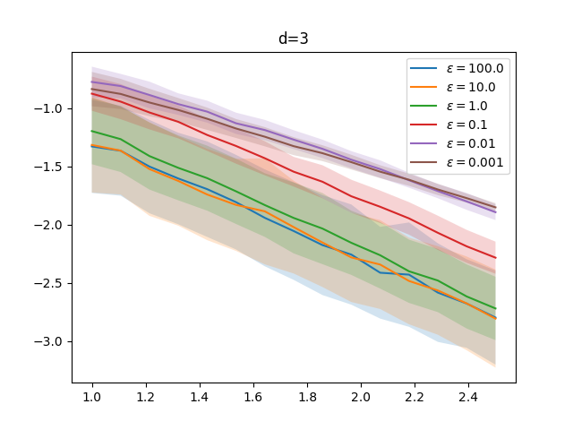
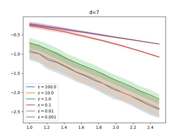
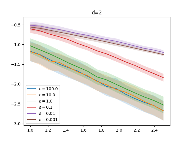
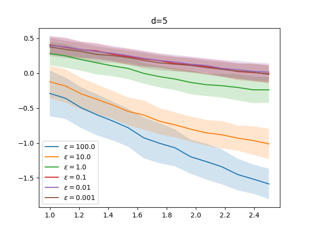
Figure 1: W¯ε(α^n,α^n)subscript¯𝑊𝜀subscript^𝛼𝑛superscriptsubscript^𝛼𝑛\bar{W}_{\varepsilon}(\hat{\alpha}_{n},\hat{\alpha}_{n}^{\prime}) as a function of n𝑛n in log-log space : Influence of ε𝜀\varepsilon for fixed d𝑑d on two uniform distributions on the hypercube with quadratic cost.
Refer to caption
Refer to caption
Refer to caption
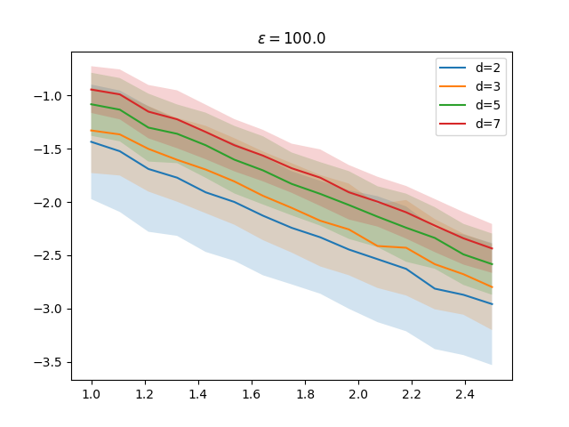
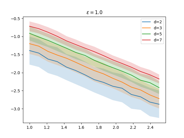
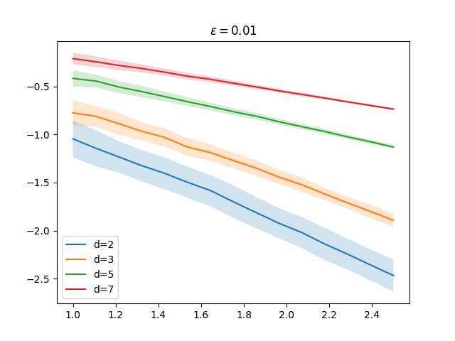
Figure 2: W¯ε(α^n,α^n)subscript¯𝑊𝜀subscript^𝛼𝑛superscriptsubscript^𝛼𝑛\bar{W}_{\varepsilon}(\hat{\alpha}_{n},\hat{\alpha}_{n}^{\prime}) as a function of n𝑛n in log-log space : Influence of d𝑑d for fixed ε𝜀\varepsilon on two uniform distributions on the hypercube with quadratic cost.
Lemma 4.

Let 𝒜={(u,v)uv2L|𝒳|+c}𝒜conditional-set𝑢𝑣direct-sum𝑢𝑣2𝐿𝒳subscriptnorm𝑐\mathcal{A}=\{(u,v)\mid u\oplus v\leqslant 2L|\mathcal{X}|+\left\|c\right\|_{\infty}\}. We have:

  • (i)

    the pairs of optimal potentials (u,v)superscript𝑢superscript𝑣(u^{*},v^{*}) such that u(0)=0superscript𝑢00u^{*}(0)=0 belong to 𝒜𝒜\mathcal{A},

  • (ii)

    fεsuperscript𝑓𝜀f^{\varepsilon} is B-Lipschitz in (u,v)𝑢𝑣(u,v) on 𝒜𝒜\mathcal{A} with B1+exp(2L|𝒳|+cε)𝐵12𝐿𝒳subscriptnorm𝑐𝜀B\leqslant 1+\exp(2\frac{L|\mathcal{X}|+\left\|c\right\|_{\infty}}{\varepsilon}).

Proof.

Let us prove that we can restrict ourselves to a subspace on which fεsuperscript𝑓𝜀f^{\varepsilon} is Lipschitz in (u,v)𝑢𝑣(u,v).

fε(u,v,x,y)=u(x)+v(y)εexp(u(x)+v(y)c(x,y)ε)superscript𝑓𝜀𝑢𝑣𝑥𝑦𝑢𝑥𝑣𝑦𝜀𝑢𝑥𝑣𝑦𝑐𝑥𝑦𝜀f^{\varepsilon}(u,v,x,y)=u(x)+v(y)-\varepsilon\exp\left(\frac{u(x)+v(y)-c(x,y)}{\varepsilon}\right)
fε(u,v)=1exp(u+vcε).superscript𝑓𝜀𝑢𝑣1𝑢𝑣𝑐𝜀\nabla f^{\varepsilon}(u,v)=1-\exp\left(\frac{u+v-c}{\varepsilon}\right).

To ensure that fεsuperscript𝑓𝜀f^{\varepsilon} is Lipschitz, we simply need to ensure that the quantity inside the exponential is upperbounded at optimality and then restrict the function to all (u,v)𝑢𝑣(u,v) that satisfy that bound.

Recall the bounds on the optimal potentials from Proposition 1. We have that x𝒳,y𝒴formulae-sequencefor-all𝑥𝒳𝑦𝒴\forall x\in\mathcal{X},y\in\mathcal{Y},

u(x)L|x|andv(y)maxxu(x)c(x,y).formulae-sequence𝑢𝑥𝐿𝑥and𝑣𝑦subscript𝑥𝑢𝑥𝑐𝑥𝑦u(x)\leqslant L|x|\quad\text{and}\quad v(y)\leqslant\max_{x}u(x)-c(x,y).

Since we assumed 𝒳𝒳\mathcal{X} to be a bounded set, denoting by |𝒳|𝒳|\mathcal{X}| the diameter of the space we get that at optimality x𝒳,y𝒴formulae-sequencefor-all𝑥𝒳𝑦𝒴\forall x\in\mathcal{X},y\in\mathcal{Y}

u(x)+v(y)2L|𝒳|+c.𝑢𝑥𝑣𝑦2𝐿𝒳subscriptnorm𝑐u(x)+v(y)\leqslant 2L|\mathcal{X}|+\left\|c\right\|_{\infty}.

Let us denote 𝒜={(u,v)(𝐇s(d))2uv2L|𝒳|+c}𝒜conditional-set𝑢𝑣superscriptsuperscript𝐇𝑠superscript𝑑2direct-sum𝑢𝑣2𝐿𝒳subscriptnorm𝑐\mathcal{A}=\{(u,v)\in(\mathbf{H}^{s}(\mathbb{R}^{d}))^{2}\mid u\oplus v\leqslant 2L|\mathcal{X}|+\left\|c\right\|_{\infty}\}, we have that (u,v)𝒜for-all𝑢𝑣𝒜\forall(u,v)\in\mathcal{A},

|fε(u,v)|1+exp(2L|𝒳|+cε).superscript𝑓𝜀𝑢𝑣12𝐿𝒳subscriptnorm𝑐𝜀|\nabla f^{\varepsilon}(u,v)|\leqslant 1+\exp(2\frac{L|\mathcal{X}|+\left\|c\right\|_{\infty}}{\varepsilon}).\qed

We now have all the required elements to prove our sample complexity result on the Sinkhorn loss, by applying Proposition 2.

Proof.

(Theorem 3) Since fεsubscript𝑓𝜀f_{\varepsilon} is Lipschitz and we are optimizing over 𝐇s(d)superscript𝐇𝑠superscript𝑑\mathbf{H}^{s}(\mathbb{R}^{d}) which is a RKHS, we can apply Proposition 2 to bound the supsupremum\sup in Lemma 3. We get:

𝔼|Wε(α,β)Wε(α^n,β^n)|32Bλn𝔼i=1nk(Xi,Xi)𝔼subscript𝑊𝜀𝛼𝛽subscript𝑊𝜀subscript^𝛼𝑛subscript^𝛽𝑛32𝐵𝜆𝑛𝔼superscriptsubscript𝑖1𝑛𝑘subscript𝑋𝑖subscript𝑋𝑖\mathbb{E}|W_{\varepsilon}(\alpha,\beta)-W_{\varepsilon}(\hat{\alpha}_{n},\hat{\beta}_{n})|\leqslant 3\frac{2B\lambda}{n}\mathbb{E}\sqrt{\sum_{i=1}^{n}k(X_{i},X_{i})}

where B1+exp(2L|𝒳|+cε)𝐵12𝐿𝒳subscriptnorm𝑐𝜀B\leqslant 1+\exp(2\frac{L|\mathcal{X}|+\left\|c\right\|_{\infty}}{\varepsilon}) (Lemma 4), λ=O(max(1,1εd/2))𝜆𝑂11superscript𝜀𝑑2\lambda=O(\max(1,\frac{1}{\varepsilon^{d/2}})) (Theorem 2). We can further bound i=1nk(Xi,Xi)superscriptsubscript𝑖1𝑛𝑘subscript𝑋𝑖subscript𝑋𝑖\sqrt{\sum_{i=1}^{n}k(X_{i},X_{i})} by nmaxx𝒳k(x,x)𝑛subscript𝑥𝒳𝑘𝑥𝑥\sqrt{n\max_{x\in\mathcal{X}}k(x,x)} where k𝑘k is the kernel associated to Hs(d)superscript𝐻𝑠superscript𝑑H^{s}(\mathbb{R}^{d}) (usually called Matern or Sobolev kernel) and thus maxx𝒳k(x,x)=k(0,0):=Ksubscript𝑥𝒳𝑘𝑥𝑥𝑘00assign𝐾\max_{x\in\mathcal{X}}k(x,x)=k(0,0):=K which doesn’t depend on n𝑛n or ε𝜀\varepsilon. Combining all these bounds, we get the convergence rate in 1n1𝑛\frac{1}{\sqrt{n}} with different asymptotic behaviors in ε𝜀\varepsilon when it is large or small. ∎

Using similar arguments, we can also derive a concentration result:

Corollary 1.

With probability at least 1δ1𝛿1-\delta,

|Wε(α,β)Wε(α^n,β^n)|6BλKn+C2log1δnsubscript𝑊𝜀𝛼𝛽subscript𝑊𝜀subscript^𝛼𝑛subscript^𝛽𝑛6𝐵𝜆𝐾𝑛𝐶21𝛿𝑛|W_{\varepsilon}(\alpha,\beta)-W_{\varepsilon}(\hat{\alpha}_{n},\hat{\beta}_{n})|\leqslant 6B\frac{\lambda K}{\sqrt{n}}+C\sqrt{\frac{2\log\frac{1}{\delta}}{n}}

where B,λ,K𝐵𝜆𝐾B,\lambda,K are defined in the proof above, and C=κ+εexp(κε)𝐶𝜅𝜀𝜅𝜀C=\kappa+\varepsilon\exp(\frac{\kappa}{\varepsilon}) with κ=2L|𝒳|+c𝜅2𝐿𝒳subscriptnorm𝑐\kappa=2L|\mathcal{X}|+\left\|c\right\|_{\infty}.

Proof.

We apply the bounded differences (Mc Diarmid) inequality to g:(x1,,xn)supu,vλs(𝔼fεXY1nfεXi,Yi):𝑔maps-tosubscript𝑥1subscript𝑥𝑛subscriptsupremum𝑢𝑣superscriptsubscript𝜆𝑠𝔼superscriptsubscript𝑓𝜀𝑋𝑌1𝑛superscriptsubscript𝑓𝜀subscript𝑋𝑖subscript𝑌𝑖g:(x_{1},\dots,x_{n})\mapsto\sup_{u,v\in\mathcal{H}_{\lambda}^{s}}(\mathbb{E}f_{\varepsilon}^{XY}-\frac{1}{n}f_{\varepsilon}^{X_{i},Y_{i}}). From Lemma 4 we get that x,yfor-all𝑥𝑦\forall x,y, fεxy(u,v)κ+εeκ/ε=def.Csuperscriptsubscript𝑓𝜀𝑥𝑦𝑢𝑣𝜅𝜀superscript𝑒𝜅𝜀superscriptdef.𝐶f_{\varepsilon}^{xy}(u,v)\leqslant\kappa+\varepsilon e^{\kappa/\varepsilon}\stackrel{{\scriptstyle\mbox{def.}}}{{=}}C, and thus, changing one of the variables in g𝑔g changes the value of the function by at most 2C/n2𝐶𝑛2C/n. Thus the bounded differences inequality gives

(|g(X1,,Xn)𝔼g(X1,,Xn)|>t)2exp(t2n2C2)𝑔subscript𝑋1subscript𝑋𝑛𝔼𝑔subscript𝑋1subscript𝑋𝑛𝑡2superscript𝑡2𝑛2superscript𝐶2\mathbb{P}\left(|g(X_{1},\dots,X_{n})-\mathbb{E}g(X_{1},\dots,X_{n})|>t\right)\leqslant 2\exp(\frac{t^{2}n}{2C^{2}})

Choosing t=C2log1δn𝑡𝐶21𝛿𝑛t=C\sqrt{\frac{2\log\frac{1}{\delta}}{n}} yields that with probability at least 1δ1𝛿1-\delta

g(X1,,Xn)𝔼g(X1,,Xn)+C2log1δn𝑔subscript𝑋1subscript𝑋𝑛𝔼𝑔subscript𝑋1subscript𝑋𝑛𝐶21𝛿𝑛g(X_{1},\dots,X_{n})\leqslant\mathbb{E}g(X_{1},\dots,X_{n})+C\sqrt{\frac{2\log\frac{1}{\delta}}{n}}

and from Theorem 3 we already have

𝔼g(X1,,Xn)=𝔼supu,vλs(𝔼fεXY1nfεXi,Yi)2BλKn.𝔼𝑔subscript𝑋1subscript𝑋𝑛𝔼subscriptsupremum𝑢𝑣superscriptsubscript𝜆𝑠𝔼superscriptsubscript𝑓𝜀𝑋𝑌1𝑛superscriptsubscript𝑓𝜀subscript𝑋𝑖subscript𝑌𝑖2𝐵𝜆𝐾𝑛\mathbb{E}g(X_{1},\dots,X_{n})=\mathbb{E}\sup_{u,v\in\mathcal{H}_{\lambda}^{s}}(\mathbb{E}f_{\varepsilon}^{XY}-\frac{1}{n}f_{\varepsilon}^{X_{i},Y_{i}})\leqslant\frac{2B\lambda K}{\sqrt{n}}.

Refer to caption
Refer to caption
Refer to caption
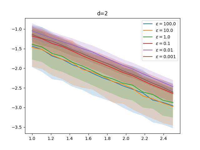
Figure 3: W¯ε(α^n,α^n)subscript¯𝑊𝜀subscript^𝛼𝑛superscriptsubscript^𝛼𝑛\bar{W}_{\varepsilon}(\hat{\alpha}_{n},\hat{\alpha}_{n}^{\prime}) as a function of n𝑛n in log-log space - cost c(x,y)=xy1𝑐𝑥𝑦subscriptnorm𝑥𝑦1c(x,y)=|\!|x-y|\!|_{1} with uniform distributions (two leftmost figures) and quadratic cost c(x,y)=xy22𝑐𝑥𝑦superscriptsubscriptnorm𝑥𝑦22c(x,y)=|\!|x-y|\!|_{2}^{2} with standard normal distributions (right figure).

6 Experiments

We conclude with some numerical experiments on the sample complexity of Sinkhorn Divergences. Since there are no explicit formulas for Wεsubscript𝑊𝜀W_{\varepsilon} in general, we consider W¯ε(α^n,α^n)subscript¯𝑊𝜀subscript^𝛼𝑛superscriptsubscript^𝛼𝑛\bar{W}_{\varepsilon}(\hat{\alpha}_{n},\hat{\alpha}_{n}^{\prime}) where α^n=def.1ni=1nδXisuperscriptdef.subscript^𝛼𝑛1𝑛superscriptsubscript𝑖1𝑛subscript𝛿𝑋𝑖\hat{\alpha}_{n}\stackrel{{\scriptstyle\mbox{def.}}}{{=}}\frac{1}{n}\sum_{i=1}^{n}\delta_{Xi}, α^n=def.1ni=1nδXisuperscriptdef.superscriptsubscript^𝛼𝑛1𝑛superscriptsubscript𝑖1𝑛subscript𝛿𝑋superscript𝑖\hat{\alpha}_{n}^{\prime}\stackrel{{\scriptstyle\mbox{def.}}}{{=}}\frac{1}{n}\sum_{i=1}^{n}\delta_{Xi^{\prime}} and (X1,,Xn)subscript𝑋1subscript𝑋𝑛(X_{1},\dots,X_{n}) and (X1,,Xn)superscriptsubscript𝑋1superscriptsubscript𝑋𝑛(X_{1}^{\prime},\dots,X_{n}^{\prime}) are two independent n𝑛n-samples from α𝛼\alpha. Note that we use in this section the normalized Sinkhorn Divergence as defined in (2), since we know that W¯ε(α,α)=0subscript¯𝑊𝜀𝛼𝛼0\bar{W}_{\varepsilon}(\alpha,\alpha)=0 and thus W¯ε(α^n,α^n)0subscript¯𝑊𝜀subscript^𝛼𝑛superscriptsubscript^𝛼𝑛0\bar{W}_{\varepsilon}(\hat{\alpha}_{n},\hat{\alpha}_{n}^{\prime})\rightarrow 0 as n+𝑛n\rightarrow+\infty .

Each of the experiments is run 300300300 times, and we plot the average of W¯ε(α^n,α^n)subscript¯𝑊𝜀subscript^𝛼𝑛superscriptsubscript^𝛼𝑛\bar{W}_{\varepsilon}(\hat{\alpha}_{n},\hat{\alpha}_{n}^{\prime}) as a function of n𝑛n in log-log space, with shaded standard deviation bars.

First, we consider the uniform distribution over a hypercube with the standard quadratic cost c(x,y)=xy22𝑐𝑥𝑦superscriptsubscriptnorm𝑥𝑦22c(x,y)=|\!|x-y|\!|_{2}^{2}, which falls within our framework, as we are dealing with a 𝒞superscript𝒞\mathcal{C}^{\infty} cost on a bounded domain. Figure 1 shows the influence of the dimension d𝑑d on the convergence, while Figure 2 shows the influence of the regularization ε𝜀\varepsilon on the convergence for a given dimension. The influence of ε𝜀\varepsilon on the convergence rate increases with the dimension: the curves are almost parallel for all values of ε𝜀\varepsilon in dimension 2 but they get further apart as dimension increases. As expected from our bound, there is a cutoff which happens here at ε=1𝜀1\varepsilon=1. All values of ε1𝜀1\varepsilon\geqslant 1 have similar convergence rates, and the dependence on 1ε1𝜀\frac{1}{\varepsilon} becomes clear for smaller values. The same cutoff appears when looking at the influence of the dimension on the convergence rate for a fixed ε𝜀\varepsilon. The curves are parallel for all dimensions for ε1𝜀1\varepsilon\geqslant 1 but they have very different slopes for smaller ε𝜀\varepsilon.

We relax next some of the assumptions needed in our theorem to see how the Sinkhorn divergence behaves empirically. First we relax the regularity assumption on the cost, using c(x,y)=xy1𝑐𝑥𝑦subscriptnorm𝑥𝑦1c(x,y)=|\!|x-y|\!|_{1}. As seen on the two left images in figure 3 the behavior is very similar to the quadratic cost but with a more pronounced influence of ε𝜀\varepsilon, even for small dimensions. The fact that the convergence rate gets slower as ε𝜀\varepsilon gets smaller is already very clear in dimension 2, which wasn’t the case for the quadratic cost. The influence of the dimension for a given value of ε𝜀\varepsilon is not any different however.

We also relax the bounded domain assumption, considering a standard normal distribution over dsuperscript𝑑\mathbb{R}^{d} with a quadratic cost. While the influence of ε𝜀\varepsilon on the convergence rate is still obvious, the influence of the dimension is less clear. There is also a higher variance, which can be expected as the concentration bound from Corollary 1 depends on the diameter of the domain.

For all curves, we observe that d𝑑d and ε𝜀\varepsilon impact variance, with much smaller variance for small values of ε𝜀\varepsilon and high dimensions. From the concentration bound, the dependency on ε𝜀\varepsilon coming from the uniform bound on fεsubscript𝑓𝜀f_{\varepsilon} is of the form εexp(κ/ε)𝜀𝜅𝜀\varepsilon\exp(\kappa/\varepsilon), suggesting higher variance for small values of ε𝜀\varepsilon. This could indicate that our uniform bound on fεsubscript𝑓𝜀f_{\varepsilon} is not tight, and we should consider other methods to get tighter bounds in further work.

7 Conclusion

We have presented two convergence theorems for SDs: a bound on the approximation error of OT and a sample complexity bound for empirical Sinkhorn divergences. The 1/n1𝑛1/\sqrt{n} convergence rate is similar to MMD, but with a constant that depends on the inverse of the regularization parameter, which nicely complements the interpolation property of SDs pointed out in recent papers. Furthermore, the reformulation of SDs as the maximization of an expectation in a RKHS ball also opens the door to a better use of kernel-SGD for the computation of SDs.

Our numerical experiments suggest some open problems. It seems that the convergence rate still holds for unbounded domains and non-smooth cost functions. Besides, getting tighter bounds in our theorem might allow us to derive a sharp estimate on the optimal ε𝜀\varepsilon to approximate OT for a given n𝑛n, by combining our two convergence theorems together.

References

  • Ambrosio et al. (2006) L. Ambrosio, N. Gigli, and G. Savaré. Gradient flows in metric spaces and in the space of probability measures. Springer, 2006.
  • Arjovsky et al. (2017) M. Arjovsky, S. Chintala, and L. Bottou. Wasserstein gan. arXiv preprint arXiv:1701.07875, 2017.
  • Bartlett and Mendelson (2002) P. L. Bartlett and S. Mendelson. Rademacher and gaussian complexities: Risk bounds and structural results. Journal of Machine Learning Research, 3(Nov):463–482, 2002.
  • Beaumont et al. (2002) M. A. Beaumont, W. Zhang, and D. J. Balding. Approximate bayesian computation in population genetics. Genetics, 162(4):2025–2035, 2002.
  • Bigot et al. (2017) J. Bigot, E. Cazelles, and N. Papadakis. Central limit theorems for sinkhorn divergence between probability distributions on finite spaces and statistical applications. arXiv preprint arXiv:1711.08947, 2017.
  • Calderón (1961) A. Calderón. Lebesgue spaces of differentiable functions. In Proc. Sympos. Pure Math, volume 4, pages 33–49, 1961.
  • Carlier et al. (2017) G. Carlier, V. Duval, G. Peyré, and B. Schmitzer. Convergence of entropic schemes for optimal transport and gradient flows. SIAM Journal on Mathematical Analysis, 49(2):1385–1418, 2017.
  • Chen et al. (2016) Y. Chen, T. Georgiou, and M. Pavon. Entropic and displacement interpolation: a computational approach using the hilbert metric. SIAM Journal on Applied Mathematics, 76(6):2375–2396, 2016.
  • Courty et al. (2014) N. Courty, R. Flamary, and D. Tuia. Domain adaptation with regularized optimal transport. In Joint European Conference on Machine Learning and Knowledge Discovery in Databases, pages 274–289. Springer, 2014.
  • Cuturi (2013) M. Cuturi. Sinkhorn distances: Lightspeed computation of optimal transport. In Adv. in Neural Information Processing Systems, pages 2292–2300, 2013.
  • Dudley (1969) R. Dudley. The speed of mean glivenko-cantelli convergence. The Annals of Mathematical Statistics, 40(1):40–50, 1969.
  • Frogner et al. (2015) C. Frogner, C. Zhang, H. Mobahi, M. Araya, and T. Poggio. Learning with a Wasserstein loss. In Adv. in Neural Information Processing Systems, pages 2044–2052, 2015.
  • Genevay et al. (2016) A. Genevay, M. Cuturi, G. Peyré, and F. Bach. Stochastic optimization for large-scale optimal transport. In D. D. Lee, U. V. Luxburg, I. Guyon, and R. Garnett, editors, Proc. NIPS’16, pages 3432–3440. Curran Associates, Inc., 2016.
  • Genevay et al. (2018) A. Genevay, G. Peyre, and M. Cuturi. Learning generative models with sinkhorn divergences. In International Conference on Artificial Intelligence and Statistics, pages 1608–1617, 2018.
  • Gretton et al. (2006) A. Gretton, K. Borgwardt, M. Rasch, B. Schölkopf, and A. Smola. A kernel method for the two-sample-problem. In Adv. in Neural Information Processing Systems, pages 513–520, 2006.
  • Kantorovich (1942) L. Kantorovich. On the transfer of masses (in Russian). Doklady Akademii Nauk, 37(2):227–229, 1942.
  • Kusner et al. (2015) M. Kusner, Y. Sun, N. Kolkin, and K. Q. Weinberger. From word embeddings to document distances. In Proc. of the 32nd Intern. Conf. on Machine Learning, pages 957–966, 2015.
  • Li et al. (2017) C.-L. Li, W.-C. Chang, Y. Cheng, Y. Yang, and B. Póczos. MMD GAN: Towards deeper understanding of moment matching network. arXiv preprint arXiv:1705.08584, 2017.
  • Li et al. (2015) Y. Li, K. Swersky, and R. Zemel. Generative moment matching networks. In International Conference on Machine Learning, pages 1718–1727, 2015.
  • Ramdas et al. (2017) A. Ramdas, N. G. Trillos, and M. Cuturi. On wasserstein two-sample testing and related families of nonparametric tests. Entropy, 19(2):47, 2017.
  • Salimans et al. (2018) T. Salimans, H. Zhang, A. Radford, and D. Metaxas. Improving GANs using optimal transport. In International Conference on Learning Representations, 2018.
  • Sriperumbudur et al. (2012) B. Sriperumbudur, K. Fukumizu, A. Gretton, B. Schoelkopf, and G. Lanckriet. On the empirical estimation of integral probability metrics. Electronic Journal of Statistics, 6:1550–1599, 2012.
  • Weed and Bach (2017) J. Weed and F. Bach. Sharp asymptotic and finite-sample rates of convergence of empirical measures in wasserstein distance. arXiv preprint arXiv:1707.00087, 2017.

Appendix

Proof.

(Lemma 1) For better clarity, we carry out the computations in dimension 1 but all the arguments are valid in higher dimension and we will clarify delicate points throughout the proof.

Differentiating both sides of the optimality condition (6) and rearranging yields

u(x)=c(x,y)γε(x,y)β(y)𝑑y.superscript𝑢𝑥superscript𝑐𝑥𝑦subscript𝛾𝜀𝑥𝑦𝛽𝑦differential-d𝑦u^{\prime}(x)=\int c^{\prime}(x,y)\gamma_{\varepsilon}(x,y)\beta(y)dy. (13)

Notice that γε(x,y)=u(x)c(x,y)εγε(x,y)superscriptsubscript𝛾𝜀𝑥𝑦superscript𝑢𝑥superscript𝑐𝑥𝑦𝜀subscript𝛾𝜀𝑥𝑦\gamma_{\varepsilon}^{\prime}(x,y)=\frac{u^{\prime}(x)-c^{\prime}(x,y)}{\varepsilon}\gamma_{\varepsilon}(x,y). Thus by immediate recurrence (differentiating both sides of the equality again) we get that

u(n)(x)=gn(x,y)γε(x,y)β(y)𝑑y,superscript𝑢𝑛𝑥subscript𝑔𝑛𝑥𝑦subscript𝛾𝜀𝑥𝑦𝛽𝑦differential-d𝑦u^{(n)}(x)=\int g_{n}(x,y)\gamma_{\varepsilon}(x,y)\beta(y)dy, (14)

where gn+1(x,y)=gn(x,y)+u(x)c(x,y)εgn(x,y)subscript𝑔𝑛1𝑥𝑦superscriptsubscript𝑔𝑛𝑥𝑦superscript𝑢𝑥superscript𝑐𝑥𝑦𝜀subscript𝑔𝑛𝑥𝑦g_{n+1}(x,y)=g_{n}^{\prime}(x,y)+\frac{u^{\prime}(x)-c^{\prime}(x,y)}{\varepsilon}g_{n}(x,y) and g1(x,y)=c(x,y)subscript𝑔1𝑥𝑦superscript𝑐𝑥𝑦g_{1}(x,y)=c^{\prime}(x,y)

To extend this first lemma to the d𝑑d-dimensional case, we need to consider the sequence of indexes σ=(σ1,σ2,){1,,d}𝜎subscript𝜎1subscript𝜎2superscript1𝑑\sigma=(\sigma_{1},\sigma_{2},\dots)\in\{1,\dots,d\}^{\mathbb{N}} which corresponds to the axis along which we successively differentiate. Using the same reasoning as above, it is straightforward to check that

kuxσ1xσk=gσ,kγεsuperscript𝑘𝑢subscript𝑥subscript𝜎1subscript𝑥subscript𝜎𝑘subscript𝑔𝜎𝑘subscript𝛾𝜀\frac{\partial^{k}u}{\partial x_{\sigma_{1}}\dots\partial x_{\sigma_{k}}}=\int g_{\sigma,k}\gamma_{\varepsilon}

where gσ,1=cxσ1subscript𝑔𝜎1𝑐subscript𝑥subscript𝜎1g_{\sigma,1}=\frac{\partial c}{\partial x_{\sigma_{1}}} and gσ,k+1=gσ,k+1xσk+1+1ε(uxσk+1cxσk+1)gσ,k+1subscript𝑔𝜎𝑘1subscript𝑔𝜎𝑘1subscript𝑥subscript𝜎𝑘11𝜀𝑢subscript𝑥subscript𝜎𝑘1𝑐subscript𝑥subscript𝜎𝑘1subscript𝑔𝜎𝑘1g_{\sigma,k+1}=\frac{\partial g_{\sigma,k+1}}{\partial x_{\sigma_{k+1}}}+\frac{1}{\varepsilon}\left(\frac{\partial u}{\partial x_{\sigma_{k+1}}}-\frac{\partial c}{\partial x_{\sigma_{k+1}}}\right)g_{\sigma,k+1}

Proof.

(Lemma 2) The proof is made by recurrence on the following property :
Pnsubscript𝑃𝑛P_{n} : For all j=0,,k𝑗0𝑘j=0,\dots,k, for all k=0,,n2𝑘0𝑛2k=0,\dots,n-2, gnk(j)subscriptnormsuperscriptsubscript𝑔𝑛𝑘𝑗\left\|g_{n-k}^{(j)}\right\|_{\infty} is bounded by a polynomial in 1ε1𝜀\frac{1}{\varepsilon} of order nk+j1𝑛𝑘𝑗1n-k+j-1.
Let us initialize the recurrence with n=2𝑛2n=2

g2subscript𝑔2\displaystyle g_{2} =\displaystyle= g1+ucεg1superscriptsubscript𝑔1superscript𝑢superscript𝑐𝜀subscript𝑔1\displaystyle g_{1}^{\prime}+\frac{u^{\prime}-c^{\prime}}{\varepsilon}g_{1} (15)
g2subscriptnormsubscript𝑔2\displaystyle\left\|g_{2}\right\|_{\infty} \displaystyle\leqslant g1+u+cεg1subscriptnormsuperscriptsubscript𝑔1subscriptnormsuperscript𝑢subscriptnormsuperscript𝑐𝜀subscriptnormsubscript𝑔1\displaystyle\left\|g_{1}^{\prime}\right\|_{\infty}+\frac{\left\|u^{\prime}\right\|_{\infty}+\left\|c^{\prime}\right\|_{\infty}}{\varepsilon}\left\|g_{1}\right\|_{\infty} (16)

Recall that u=g1=csubscriptnormsuperscript𝑢subscriptnormsubscript𝑔1subscriptnormsuperscript𝑐\left\|u^{\prime}\right\|_{\infty}=\left\|g_{1}\right\|_{\infty}=\left\|c^{\prime}\right\|_{\infty}. Let C=maxkc(k)𝐶subscript𝑘subscriptnormsuperscript𝑐𝑘C=\max_{k}\left\|c^{(k)}\right\|_{\infty}, we get that g2C+C+CεCsubscriptnormsubscript𝑔2𝐶𝐶𝐶𝜀𝐶\left\|g_{2}\right\|_{\infty}\leqslant C+\frac{C+C}{\varepsilon}C which is of the required form.

Now assume that Pnsubscript𝑃𝑛P_{n} is true for some n2𝑛2n\geqslant 2. This means we have bounds on gnk(i)superscriptsubscript𝑔𝑛𝑘𝑖g_{n-k}^{(i)}, for k=0,,n2𝑘0𝑛2k=0,\dots,n-2 and i=0,,k𝑖0𝑘i=0,\dots,k. To prove the property at rank n+1𝑛1n+1 we want bounds on gn+1k(i)superscriptsubscript𝑔𝑛1𝑘𝑖g_{n+1-k}^{(i)}, for k=0,,n1𝑘0𝑛1k=0,\dots,n-1 and i=0,,k𝑖0𝑘i=0,\dots,k. The only new quantity that we need to bound are gn+1k(k),k=0,,n1formulae-sequencesuperscriptsubscript𝑔𝑛1𝑘𝑘𝑘0𝑛1g_{n+1-k}^{(k)},k=0,\dots,n-1. Let us start by bounding g2(n1)superscriptsubscript𝑔2𝑛1g_{2}^{(n-1)} which corresponds to k=n1𝑘𝑛1k=n-1 and we will do a backward recurrence on k𝑘k. By applying Leibniz formula for the successive derivatives of a product of functions, we get

g2subscript𝑔2\displaystyle g_{2} =\displaystyle= g1+ucεg1superscriptsubscript𝑔1superscript𝑢superscript𝑐𝜀subscript𝑔1\displaystyle g_{1}^{\prime}+\frac{u^{\prime}-c^{\prime}}{\varepsilon}g_{1} (17)
g2(n1)superscriptsubscript𝑔2𝑛1\displaystyle g_{2}^{(n-1)} =\displaystyle= g1(n)+p=0n1(n1p)u(p+1)c(p+1)εg1(n1p)superscriptsubscript𝑔1𝑛superscriptsubscript𝑝0𝑛1binomial𝑛1𝑝superscript𝑢𝑝1superscript𝑐𝑝1𝜀superscriptsubscript𝑔1𝑛1𝑝\displaystyle g_{1}^{(n)}+\sum_{p=0}^{n-1}\binom{n-1}{p}\frac{u^{(p+1)}-c^{(p+1)}}{\varepsilon}g_{1}^{(n-1-p)} (18)
g2(n1)subscriptnormsuperscriptsubscript𝑔2𝑛1\displaystyle\left\|g_{2}^{(n-1)}\right\|_{\infty} \displaystyle\leqslant g1(n)+p=0n1(n1p)u(p+1)+c(p+1)εg1(n1p)subscriptnormsuperscriptsubscript𝑔1𝑛superscriptsubscript𝑝0𝑛1binomial𝑛1𝑝subscriptnormsuperscript𝑢𝑝1subscriptnormsuperscript𝑐𝑝1𝜀subscriptnormsuperscriptsubscript𝑔1𝑛1𝑝\displaystyle\left\|g_{1}^{(n)}\right\|_{\infty}+\sum_{p=0}^{n-1}\binom{n-1}{p}\frac{\left\|u^{(p+1)}\right\|_{\infty}+\left\|c^{(p+1)}\right\|_{\infty}}{\varepsilon}\left\|g_{1}^{(n-1-p)}\right\|_{\infty} (19)
\displaystyle\leqslant C+p=0n1(n1p)gp+1+CεC𝐶superscriptsubscript𝑝0𝑛1binomial𝑛1𝑝subscriptnormsubscript𝑔𝑝1𝐶𝜀𝐶\displaystyle C+\sum_{p=0}^{n-1}\binom{n-1}{p}\frac{\left\|g_{p+1}\right\|_{\infty}+C}{\varepsilon}C (20)

Thanks to Pnsubscript𝑃𝑛P_{n} we have that gpi=0pai,p1εi,p=1,,nformulae-sequencesubscriptnormsubscript𝑔𝑝superscriptsubscript𝑖0𝑝subscript𝑎𝑖𝑝1superscript𝜀𝑖𝑝1𝑛\left\|g_{p}\right\|_{\infty}\leqslant\sum_{i=0}^{p}a_{i,p}\frac{1}{\varepsilon^{i}},p=1,\dots,n so the highest order term in ε𝜀\varepsilon in the above inequality is 1εn1superscript𝜀𝑛\frac{1}{\varepsilon^{n}}. Thus we get g2(n1)i=0n+1ai,2,n11εisubscriptnormsuperscriptsubscript𝑔2𝑛1superscriptsubscript𝑖0𝑛1subscript𝑎𝑖2𝑛11superscript𝜀𝑖\left\|g_{2}^{(n-1)}\right\|_{\infty}\leqslant\sum_{i=0}^{n+1}a_{i,2,n-1}\frac{1}{\varepsilon^{i}} which is of the expected order

Now assume gn+1j(j)superscriptsubscript𝑔𝑛1𝑗𝑗g_{n+1-j}^{(j)} are bounded with the appropriate polynomials for j<kn1𝑗𝑘𝑛1j<k\leqslant n-1. Let us bound gn+1k(k)superscriptsubscript𝑔𝑛1𝑘𝑘g_{n+1-k}^{(k)}

gn+1k(k)subscriptnormsuperscriptsubscript𝑔𝑛1𝑘𝑘\displaystyle\left\|g_{n+1-k}^{(k)}\right\|_{\infty} \displaystyle\leqslant gnk(k+1)+p=0k(kp)u(p+1)+c(p+1)εgnk(kp)subscriptnormsuperscriptsubscript𝑔𝑛𝑘𝑘1superscriptsubscript𝑝0𝑘binomial𝑘𝑝subscriptnormsuperscript𝑢𝑝1subscriptnormsuperscript𝑐𝑝1𝜀subscriptnormsuperscriptsubscript𝑔𝑛𝑘𝑘𝑝\displaystyle\left\|g_{n-k}^{(k+1)}\right\|_{\infty}+\sum_{p=0}^{k}\binom{k}{p}\frac{\left\|u^{(p+1)}\right\|_{\infty}+\left\|c^{(p+1)}\right\|_{\infty}}{\varepsilon}\left\|g_{n-k}^{(k-p)}\right\|_{\infty} (21)
\displaystyle\leqslant gnk(k+1)+p=0k(kp)gp+1+Cεgnk(kp)subscriptnormsuperscriptsubscript𝑔𝑛𝑘𝑘1superscriptsubscript𝑝0𝑘binomial𝑘𝑝subscriptnormsubscript𝑔𝑝1𝐶𝜀subscriptnormsuperscriptsubscript𝑔𝑛𝑘𝑘𝑝\displaystyle\left\|g_{n-k}^{(k+1)}\right\|_{\infty}+\sum_{p=0}^{k}\binom{k}{p}\frac{\left\|g_{p+1}\right\|_{\infty}+C}{\varepsilon}\left\|g_{n-k}^{(k-p)}\right\|_{\infty} (22)

The first term gnk(k+1)subscriptnormsuperscriptsubscript𝑔𝑛𝑘𝑘1\left\|g_{n-k}^{(k+1)}\right\|_{\infty} is bounded with a polynomial of order 1εn+11superscript𝜀𝑛1\frac{1}{\varepsilon^{n+1}} by recurrence assumption. Regarding the terms in the sum, they also have all been bounded and

gp+1gnk(kp)(i=0pai,p+11εi)(i=0npai,nk,kp1εi)i=0na~i1εisubscriptnormsubscript𝑔𝑝1subscriptnormsuperscriptsubscript𝑔𝑛𝑘𝑘𝑝superscriptsubscript𝑖0𝑝subscript𝑎𝑖𝑝11superscript𝜀𝑖superscriptsubscript𝑖0𝑛𝑝subscript𝑎𝑖𝑛𝑘𝑘𝑝1superscript𝜀𝑖superscriptsubscript𝑖0𝑛subscript~𝑎𝑖1superscript𝜀𝑖\left\|g_{p+1}\right\|_{\infty}\left\|g_{n-k}^{(k-p)}\right\|_{\infty}\leqslant\left(\sum_{i=0}^{p}a_{i,p+1}\frac{1}{\varepsilon^{i}}\right)\left(\sum_{i=0}^{n-p}a_{i,n-k,k-p}\frac{1}{\varepsilon^{i}}\right)\leqslant\sum_{i=0}^{n}\tilde{a}_{i}\frac{1}{\varepsilon^{i}}

So gn+1k(k)i=0n+1ai,n+1k,k1εisubscriptnormsuperscriptsubscript𝑔𝑛1𝑘𝑘superscriptsubscript𝑖0𝑛1subscript𝑎𝑖𝑛1𝑘𝑘1superscript𝜀𝑖\left\|g_{n+1-k}^{(k)}\right\|_{\infty}\leqslant\sum_{i=0}^{n+1}a_{i,n+1-k,k}\frac{1}{\varepsilon^{i}}

To extend the result in dsuperscript𝑑\mathbb{R}^{d}, the recurrence is made on the the following property

gσ,nk(j)i=0nk+|j|1ai,nk,j,σ1εij|j|=0,,kk=0,,n2σ{1,,d}\left\|g_{\sigma,n-k}^{(j)}\right\|_{\infty}\leqslant\sum_{i=0}^{n-k+|j|-1}a_{i,n-k,j,\sigma}\frac{1}{\varepsilon^{i}}\qquad\forall j\mid|j|=0,\dots,k\quad\forall k=0,\dots,n-2\quad\forall\sigma\in\{1,\dots,d\}^{\mathbb{N}} (23)

where j𝑗j is a multi-index since we are dealing with multi-variate functions, and gσ,nksubscript𝑔𝜎𝑛𝑘g_{\sigma,n-k} is defined at the end of the previous proof. The computations can be carried out in the same way as above, using the multivariate version of Leibniz formula in (18) since we are now dealing with multi-indexes. ∎