Estimation of parameters in circuit QED by continuous quantum measurement

Abstract

Designing high-precision and efficient protocols is of crucial importance for quantum parameter estimation in practice. Estimation based on continuous quantum measurement is one possible type of this, which also appears to be the most natural choice for continuous dynamical processes. In this work we consider the state-of-the-art superconducting circuit quantum-electrodynamics (QED) systems, where high-quality continuous measurements have been extensively performed in the past decade. Within the framework of Bayesian estimation and particularly using the quantum Bayesian rule in circuit QED, we numerically simulate the likelihood function as estimator for the Rabi frequency of qubit oscillations. We find that, by proper design of the interaction strength of measurement, the estimate precision can scale with the measurement time beyond the standard quantum limit, which is usually assumed for this type of continuous measurement. This unexpected result is supported by the simulated Fisher information, and can be understood as a consequence of the quantum correlation between the output signals by simulating the effect of quantum efficiency of measurement.

I Introduction

The problem of accurately estimating unknown parameters is of both theoretical interest and of practical importance He69 ; Ho11 . In order to minimize the estimation uncertainties, a variety of strategies have been developed in the science of quantum metrology over the past decades GLM04 ; GLM11 ; Dem15 . In this context, a central topic is how to exploit quantum techniques to achieve parameter estimation with precision beyond that obtainable by any classical scheme GLM04 ; GLM11 ; Dem15 . For example, if a system is initially prepared in a spin coherent state, the precision of frequency estimation scales with the total spin number $N$, as $1/\sqrt{N}$ which is referred to standard-quantum-limit (SQL). However, if extra quantum resources such as spin squeezing or entanglement are exploited, an enhanced precision can be achieved approaching the ultimate Heisenberg-limit (HL) scaling ($\sim 1/N$) Win92 ; Win96 .

For the theory of quantum parameter estimation, the concept of quantum Fisher information Hels76 ; Cav94 and the associated quantum Cramér-Rao bound (CRB) Cra46 ; Rao45 have been developed to set the minimum variance for unbiased estimation strategies based on measurements. However, it is not obvious how to design appropriate/optimal scheme of measurement. For different measurement schemes, which is usually characterized by a specific POVM or estimator, the associated Fisher Information would set different bound of precision according to the Cramér-Rao inequality. Designing high-precision and efficient scheme of measurement is thus of crucial importance for parameter estimation in practice.

Owing to the practical use and the rich underlying physics, in the past years there have been considerable interests in the quantum estimation of parameters using the output signals of continuous measurement Jac11 ; Molm13 ; Molm14 ; Molm15 ; Molm16 ; Jor17 ; Par17 ; Gen17 . This is also the most natural choice for parameter estimation in continuous dynamical process. This scheme has the obvious advantage of a high efficiency — unlike the conventional ensemble measurement in quantum theory, it does not need to generate the identical copies of quantum system in order to extract meaningful results from measurements. Following the seminal work Jac11 , the subsequent studies by Mølmer et al Molm13 ; Molm14 ; Molm15 ; Molm16 formulated the parameter estimation based on continuous measurement as a Bayesian scheme, for the specific example of fluorescence radiation from two-level atoms. More recently, the same problem was investigated with a focus on how to speed up the estimation by avoiding numerically integrating the stochastic master equation Jor17 . This type of parameter estimation has also been considered to include the technique of quantum smoothing MT09a ; MT09b ; MT10 ; MT15 , as a generalization of the classical signal smoothing.

In the present work, we extend the research further to the superconducting circuit quantum-electrodynamics (QED) system Bla04 ; Sch04 ; Sch08 , which is one of the leading platforms for quantum information processing and for quantum measurement and control studies. Particularly, sound studies have been performed for continuously tracking the stochastic evolution of the qubit state in this system, say, tracking the so-called quantum trajectories (QT) DiCa13 ; Dev13a ; Dev13 ; Sid13 ; Sid15 ; Sid12 . On the theoretical side, the quantum Bayesian rule has been well developed for circuit QED in the past years Kor11 ; Kor16 ; Li14 ; Li16 ; Li18 , in some cases promising the advantage of being more efficient than numerically integrating the quantum trajectory equation Gam08 ; WM09 ; Jac14 . Therefore, within the framework of Bayesian parameter estimation Molm13 ; Molm14 ; Molm15 ; Molm16 ; Jor17 , it seems a perfect choice for us to employ the quantum Bayesian rule of circuit QED for state update associated with the continuous measurement. For parameter estimation, the quantum Bayesian approach can make the calculation of the associated likelihood function very straightforward and quite efficient Jor17 , i.e., using the accumulated output currents over relatively large time interval.

In this work we perform direct simulation for large number of estimations to extract the statistical errors. Our simulation is based on the realistic (and ‘standard’) dispersive readout in circuit QED system. We investigate the effects of measurement strength, measurement time (processing time $T$ of data collection), and quantum efficiency of the measurement. As expected, we find that the estimate precision is improved with increasing $T$. However, interesting and surprisingly, we find that by proper adjustment of the measurement strength, the estimate precision can exceed the standard quantum limit, manifesting a scaling behavior with $T$ in between the SQL ($1/\sqrt{T}$) and HL ($1/T$). This result differs from what has been assumed for similar estimation of this type Molm13 ; Molm14 ; Molm15 ; Molm16 ; Jor17 , where the SQL scaling was concluded. We attribute the reason for our result to quantum correlation between the output signals of the measurement Leg85 ; Pala10 . This type of correlation in time shares some nature with the quantum entanglement Pala10 , while the latter (as a unique quantum resource) can usually result in precision better than SQL. We may also relate this understanding with the hints from extreme cases such as vanishing probe interaction Molm14 ; Molm16 ; Gut11 and dynamical phase transition Gar13 ; Gar16 , which can result in precision with Heisenberg scaling owing to the quantum correlation in time.

II Bayesian Rule in circuit QED

Let us consider a superconducting qubit coupled to a waveguide cavity, i.e., the circuit-QED architecture. In the dispersive regime, the qubit-cavity interaction is well described by the Hamiltonian Bla04 ; Sch04 , $H_{\rm int}=\chi a^{\dagger}a\sigma_{z}$, where $\chi$ is the dispersive coupling strength, $a^{\dagger}$ and $a$ are the creation and annihilation operators of the cavity mode, and $\sigma_{z}$ is the qubit Pauli operator. Associated with single quadrature homodyne measurement for microwave transmission/reflection, the output current can be reexpressed as (after the so-called polaron transformation to eliminate the degrees of freedom of the cavity photons) Li14 ; Li16 ; Li18 ; Gam08

$$I(t)=-\sqrt{\Gamma_{ci}(t)}\langle\sigma_{z}\rangle+\xi(t).$$ (1)

In this result, $\xi(t)$, originated from the fundamental quantum-jumps, is a Gaussian white noise and satisfies the ensemble-average property $E[\xi(t)]=0$ and $E[\xi(t)\xi(t^{\prime})]=\delta(t-t^{\prime})$. $\Gamma_{ci}(t)$ is the coherent information gain rate which, together with, say, the no-information back-action rate $\Gamma_{ba}(t)$ and the overall measurement decoherence rate $\Gamma_{d}(t)$, is given by

$$\Gamma_{ci}(t)=\kappa|\beta(t)|^{2}\cos^{2}(\varphi-\theta_{\beta})\,,$$ (2a)

$$\Gamma_{ba}(t)=\kappa|\beta(t)|^{2}\sin^{2}(\varphi-\theta_{\beta})\,,$$ (2b)

$$\Gamma_{d}(t)=4\chi\mathrm{Im}[\alpha^{*}_{1}(t)\alpha_{2}(t)]\,.$$ (2c)

Here $\varphi$ is the local oscillator’s (LO) phase in the homodyne measurement, $\kappa$ is the leaky rate of the microwave photon from the cavity, and $\beta(t)=\alpha_{2}(t)-\alpha_{1}(t)\equiv|\beta(t)|e^{i\theta_{\beta}}$ with $\alpha_{1}(t)$ and $\alpha_{2}(t)$ the cavity fields associated with the qubit states $|1\rangle$ and $|2\rangle$, respectively.

More detailed discussions of the physical meanings of the above rates can be found in Refs. Li14 ; Li16 ; Li18 ; Gam08 . Briefly speaking, the information-gain rate $\Gamma_{ci}$ is associated with inferring the qubit state $|e\rangle$ or $|g\rangle$ from the output current of measurement, while $\Gamma_{ba}$ characterizes the backaction of measurement not associated with the qubit-state-information gain, but rather with the qubit-level fluctuations. $\Gamma_{d}$ corresponds to the overall decoherence rate after ensemble-averaging a large number of quantum trajectories. The sum of the former two rates, $\Gamma_{m}=\Gamma_{ci}+\Gamma_{ba}$, is the total measurement rate. If $\Gamma_{m}=\Gamma_{d}$, the measurement is ideally quantum limited, with quantum efficiency $\eta=\Gamma_{m}/\Gamma_{d}=1$. Otherwise, if $\Gamma_{m}<\Gamma_{d}$, the measurement is not ideal, implying some information loss.

In steady state, the cavity fields read

$$\bar{\alpha}_{1,2}=-\epsilon_{m}[(\Delta_{r}\pm\chi)-i\kappa/2]^{-1}\,,$$ (3)

where $\Delta_{r}$ is the frequency offset between the measuring microwave (with amplitude $\epsilon_{m}$) and the cavity mode. In this work, rather than considering a general set-up of the circuit-QED system Kor16 ; Li14 ; Li16 , we restrict considerations to the bad-cavity and weak-response limits. Under this condition, the transient process of $\alpha_{1}(t)$ and $\alpha_{2}(t)$ is not important. All the rates shown above can be calculated with the steady-state fields $\bar{\alpha}_{1,2}$ given by Eq. (3).

Corresponding to the qubit state $|1\rangle$ ($|2\rangle$) and after averaging the continuous current over time interval $\tau$, i.e., ${\cal I}_{m}=(1/\tau)\int^{t+\tau}_{t}dt^{\prime}I(t^{\prime})$, the coarse-grained output current ${\cal I}_{m}$ is a stochastic variable centered at $\bar{I}_{1(2)}=\mp\sqrt{\Gamma_{ci}}$ and satisfies the Gaussian distribution with probability

$$P_{1(2)}(\tau)=(2\pi V)^{-1/2}\exp\left[-({\cal I}_{m}-\bar{I}_{1(2)})^{2}/(2V)\right],$$ (4)

where $V=1/\tau$ is the distribution variance.

Now consider an arbitrary quantum superposed state $\rho(t)$ (at the moment $t$). Based on the subsequent (coarse-grained) current $I_{m}$, the quantum Bayesian rule updates the qubit state as follows Kor11 ; Kor16 ; Li14 ; Li16 . For the diagonal elements,

$$\rho_{jj}(t+\tau)=\rho_{jj}(t)\,P_{j}(\tau)/{\cal N}(\tau)\,,$$ (5a)

where $$j=1,2 {\cal N}(\tau)=\rho_{11}(t)P_{1}(\tau)+\rho_{22}(t)P_{2}(\tau)$$ and . This is nothing but the Bayes’ theorem in probability theory. For the off-diagonal elements, which are unique in quantum theory,

$$\rho_{12}(t+\tau)=\rho_{12}(t)\left[\sqrt{P_{1}(\tau)P_{2}(\tau)}/{\cal N}(\tau)\right]$$

$$~{}~{}~{}~{}~{}~{}\times D(\tau)\,\exp\left\{-i[\Phi_{1}(\tau)+\Phi_{2}(\tau)]\right\}\,.$$ (5b)

In this result, the purity factor reads $D(\tau)=e^{-(\Gamma_{d}-\Gamma_{m})\,\tau/2}$. We remind the reader that the measurement rate is given by $\Gamma_{m}=\Gamma_{ci}+\Gamma_{ba}$. Using the steady-state solutions, Eq. (3), one can easily prove that $\Gamma_{d}=\Gamma_{m}$. Thus, in the bad-cavity limit (no transient dynamics of the cavity field), the intrinsic $D$-factor in the successive Bayesian update can be approximated by unity. In order to account for decoherence of external origins (such as photon loss and/or amplifier’s noise), one can simply introduce an extra rate $\Gamma_{\varphi}$, thus $D(\tau)=e^{-\Gamma_{\varphi}\,\tau/2}$.

The first phase factor in Eq. (5), $e^{-i\Phi_{1}(\tau)}$, is associated with an ac-Stark-shift modified unitary phase accumulation, i.e., with $\Phi_{1}(\tau)=(\Omega_{q}+B)\tau$ where the ac-Stark-shift of the qubit energy ($\Omega_{q}$) reads $B=2\chi{\rm Re}(\bar{\alpha}_{1}\bar{\alpha}^{*}_{2})$. Of more interest is the second phase factor $e^{-i\Phi_{2}(\tau)}=e^{i\Gamma_{ba}(I_{m}\tau)}$, which is associated with the accumulated random ‘charge’ and reflects the no-information gain backaction on the qubit. For a more detailed discussion on this stochastic phase factor the reader is referred to Refs. Kor11 ; Kor16 ; Li14 ; Li16 .

III Method

We assume now that the superconducting qubit is subject to a Rabi drive and at the same time subject to continuous measurement. Our goal is to estimate the Rabi frequency from the output current of the continuous measurement. The stochastic evolution of the qubit (the quantum trajectory) is governed by the following iterative rule

$$\rho(t_{j})={\cal U}_{j}{\cal M}_{j}[\rho(t_{j-1})]\,,\hskip 5.69046pt{\rm with}~{}~{}j=1,2,\cdots N\,.$$ (6)

Here we have discretized the evolution with time interval $\tau$, with thus a total measurement time $T=N\,\tau$. The superoperator ${\cal M}_{j}$ accounts for the measurement-induced change of the qubit state, whose performance is explicitly given by the quantum Bayesian rule. The superoperator ${\cal U}_{j}$ in Eq. (6) describes the unitary evolution caused by the Rabi drive, i.e., ${\cal U}_{j}(\cdots)=e^{-i{\cal L}_{q}\tau}(\cdots)=e^{-i\tilde{H}_{q}\tau}(\cdots)e^{i\tilde{H}_{q}\tau}$ with $\tilde{H}_{q}$ the qubit Hamiltonian under Rabi drive and renormalized by the measurement (i.e. with the ac-Stark shift). For small $\tau$, the action order of ${\cal U}_{j}$ and ${\cal M}_{j}$ is irrelevant.

Based on the rule of Eq. (6), we know the qubit state $\rho(t_{j})$ after the $j_{\rm th}$ step evolution, conditioned on the coarse-grained current ${\cal I}_{j}$. Meanwhile, for this $j_{\rm th}$ step of measurement, the probability of getting ${\cal I}_{j}$ is

$${\cal P}({\cal I}_{j})=\rho_{11}(t_{j-1})P_{1}(\tau)+\rho_{22}(t_{j-1})P_{2}(\tau)\,,$$ (7)

with $P_{1}(\tau)$ and $P_{2}(\tau)$ given by Eq. (4). Then, straightforwardly, the joint probability of getting the results $\{{\cal I}_{1},{\cal I}_{2},\cdots{\cal I}_{N}\}$ is simply a product of the individual probabilities

$${\cal P}(\{{\cal I}_{1},{\cal I}_{2},\cdots{\cal I}_{N}\}|\Omega)=\prod^{N}_{j=1}{\cal P}({\cal I}_{j})\,.$$ (8)

Here we explicitly indicate that this probability depends on the parameter $\Omega$ (the possible Rabi frequency).

We expect, from simple intuition, that the true Rabi frequency $\Omega_{R}$ will be most compatible with the output results $\{{\cal I}_{1},{\cal I}_{2},\cdots{\cal I}_{N}\}$, leading thus to maximum probability. Therefore, it is plausible that we get an estimate value $\Omega_{ML}$ for $\Omega_{R}$ from the location of the maximum of the probability function ${\cal P}(\{{\cal I}_{1},{\cal I}_{2},\cdots{\cal I}_{N}\}|\Omega)$, referred to in the literature as the likelihood function. Using a different $\Omega$ (rather than $\Omega_{R}$) to calculate ${\cal P}(\{{\cal I}_{1},{\cal I}_{2},\cdots{\cal I}_{N}\}|\Omega)$, based on Eqs. (6)-(8), should result in a smaller probability. This constitutes the basic idea of the maximum-likelihood-estimation (MLE) method.

Essentially, the MLE method is a Bayesian approach for parameter estimation. One may imagine, to start with, a uniform distribution ${\cal P}(\Omega)$ over a certain range. The uniform distribution means that we have no knowledge about $\Omega_{R}$. After getting the data record of measurement and performing the Bayesian inference, the knowledge about $\Omega_{R}$ changes to a new probability ${\cal P}(\Omega|{\cal I}_{1},\cdots,{\cal I}_{N})$. The peak of this new distribution can also be an estimate for $\Omega_{R}$, which should correspond to the estimated value $\Omega_{ML}$ from the MLE method.

In practice, the following log-likelihood function is used for the parameter estimation

$$L(\Omega)=\ln\,{\cal P}(\{{\cal I}_{1},{\cal I}_{2},\cdots{\cal I}_{N}\}|\Omega)\,,$$ (9)

in order to make the maximum peak more prominent. In Fig. 1, we plot this function to illustrate the MLE method (using dimensionless units here and in remainder of this work). $L(\Omega)$ is computed using the single realization of continuous measurement current $I(t)$ over $(0,T)$, by coarse-graining it into $\{{\cal I}_{1},{\cal I}_{2},\cdots,{\cal I}_{N}\}$ with $N=T/\tau$. Notice that this splitting can be rather arbitrary, i.e., with $L(\Omega)$ not influenced by the choice of $\tau$. The only requirement is that $\tau$ should not be too large to violate the precision of the Bayesian update (in the presence of Rabi oscillation). In the whole simulations of this work, we choose $\tau=1000\,dt=10^{-3}\tau_{R}$, while the time increment $dt=10^{-6}\tau_{R}$ is set for simulating the quantum trajectory equation Li14 ; Li16 ; Li18 ; Gam08 to generate the continuous output current. Through the whole work, the Rabi period ($\tau_{R}=2\pi/\Omega_{R}$) is used as the units of time. Again, we mention that the $\Omega$ dependence of $L(\Omega)$ is introduced through the unitary operator $e^{-i{\cal L}_{q}\tau}$ in each step of state update.

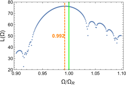
Figure 1: Illustration of the estimation method. The likelihood function is calculated (with un-normalized probability functions $P_{1,2}(\tau)$ in Eq. (7), ‘separated’ from Eq. (4)) using the quantum Bayesian rule by choosing the coarse-grained time $\tau=1000\,dt=10^{-3}\tau_{R}$, while $dt=10^{-6}\tau_{R}$ is set for simulating the quantum trajectory equation to generate the continuous output current (for time $T=N\,\tau$ with $N=10^{5}$). Through the whole work we assume the true Rabi frequency $\Omega_{R}/2\pi=1.0$ (in arbitrary dimensionless units), and accordingly we use the Rabi period $\tau_{R}=2\pi/\Omega_{R}$ as the units of time. In this plot we set the measurement strength $\Gamma_{m}=0.25\Omega_{R}$ and obtain the estimated value $\Omega_{ML}=0.992\Omega_{R}$ from the position of the maximum of the peak.

We consider a resonant Rabi drive with true Rabi frequency $\Omega_{R}/2\pi=1$ (in arbitrary dimensionless units). In the present proof-of-principle simulation, we assume $\Delta_{r}=0$ (thus $\theta_{\beta}=0$) and consider the maximal information gain with LO phase $\varphi=0$. Therefore we have $\Gamma_{ba}=0$, $\Gamma_{m}=\Gamma_{ci}$ and $\Gamma_{d}=\Gamma_{m}$ (owing to the bad-cavity limit). Except for the data shown in Fig. 4, we also do not account for any external decoherence in our simulation (setting $\Gamma_{\varphi}=0$).

Indeed, as shown in Fig. 1, we get an estimation for the Rabi frequency at $\Omega_{ML}=0.992\Omega_{R}$, from the maximum peak position of $L(\Omega)$. In this plot, we only show the log-likelihood function for a relatively small range of $\Omega$, indicating that we already have some prior knowledge about $\Omega_{R}$. If we had poor knowledge about $\Omega_{R}$, we should calculate $L(\Omega)$ for a wider range. In this case, more peaks may appear in $L(\Omega)$. An even worse situation would arise if the maximum peak would not occur near $\Omega_{R}$. This would imply a failure of the estimation and the result should be discarded.

Another point is that, in order to get a convergent estimation, one should sample a relatively large number of currents $\{{\cal I}_{1},{\cal I}_{2},\cdots,{\cal I}_{N}\}$, i.e., with large $N$ or more precisely large $T$ by noting that $T=N\tau$. Actually, it has been noted that the MLE result can saturate the Cramér-Rao bound when $N$ is large enough Molm13 ; Molm14 ; Molm15 ; Molm16 . However, the classical Cramér-Rao bound is determined by the classical Fisher information which is associated with specific schemes of measurement. It has been well understood that the more sensitive dependence of the output results on the parameter will result in better precision. Searching for an optimal measurement protocol in practice is thus of crucial importance but is unclear in general. In the following, in Fig. 2, we will further discuss this point.

A final remark is that possible quantum correlation effect may be contained in the likelihood function $L(\Omega)$. This is in some sense similar to the reason of violating the Leggett-Garg inequality (a type of Bell’s inequality in time) Leg85 as demonstrated in this same circuit-QED system via continuous measurements Pala10 . We will come back to this point later after displaying the result beyond the standard quantum limit.

IV Results

To characterize the estimation errors, we introduce the root-mean-square (RMS) variance

$$\delta\Omega=\left(\sum^{M}_{k=1}(\Omega^{(k)}_{ML}-\bar{\Omega}_{ML})^{2}\,/\,M\right)^{1/2}\,,$$ (10)

where $\bar{\Omega}_{ML}=\frac{1}{M}\sum^{M}_{k=1}\Omega^{(k)}_{ML}$, with $\Omega^{(k)}_{ML}$ the estimated result of the $k_{\rm th}$ realization based on $\{{\cal I}_{1},\cdots,{\cal I}_{N}\}^{(k)}$. To extract the RMS variance, we simulate $M=2000$ trajectories for each given measurement time ($T=N\tau$).

Let us analyze the problem of appropriate measurement, in a sense to make the measurement results more sensitive to the parameter under estimation. First, as mentioned above, we should eliminate the “realistic” (no information gain) backaction in order to maximize the information-gain rate ($\Gamma_{ci}\to\Gamma_{m}$) by adjusting the LO phase $\varphi=\theta_{\beta}=0$. Second, we search for an optimal strength for the continuous measurement, which can be characterized by the measurement rate $\Gamma_{m}$.

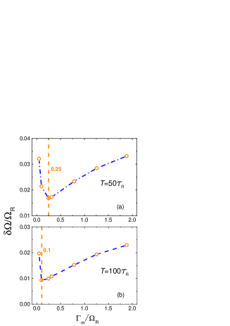
Figure 2: Measurement strength dependence of the estimation errors (root-mean-square variance). Owing to competition between information gain and measurement backaction, there exists an optimal measurement strength. The optimal strength is of $T$ dependence, as shown in (a) and (b) for $T/\tau_{R}=50$ and 100 ($\tau_{R}$ is the Rabi period). However, for longer $T$ as shown in (b), the sub-optimal $\Gamma_{m}$ (near the optimal strength) can result in good estimation with precision not very sensitive to $\Gamma_{m}$ (in the sub-optimal range).

In Fig. 2(a) we show the estimation RMS variance versus the measurement strength. Importantly, we observe the existence of an optimal strength of the continuous measurement. We understand the reason as follows. From the continuous output current Eq. (1), we know that for weak strength of measurement, the noise component (the second term) will be much larger than the information-carrying term (the first one). In other words, the output current carries little information of the qubit state which is governed by the parameter of Rabi frequency. In the other extreme, for strong strength of measurement, while the state-information-carrying component (the first term in Eq. (1)) is enhanced, the Rabi oscillation of the qubit state will be more seriously destroyed by the measurement backaction, making thus the first term of Eq. (1) not well correlated with the Rabi frequency. That is, the enhanced strength of measurement will gradually force the evolution into the so-called Zeno regime, resulting in output current of telegraphic type which is poorly correlated with the unitary Rabi drive. Therefore, it is the competition between the information-gain and measurement backaction that results in the optimal measurement strength as revealed in Fig. 2(a). From Fig. 2(b), we also find this ‘optimal’ strength not universal, but weakly depending on the measurement time $T$ (the size of the collected current). For longer measurement time, the optimal strength of measurement is smaller. However, from Fig. 2(b), we see that the ‘sub-optimal’ strength (e.g. $\Gamma_{m}/\Omega_{R}=0.25$ rather than 0.1) has little importance for the precision of the estimation.

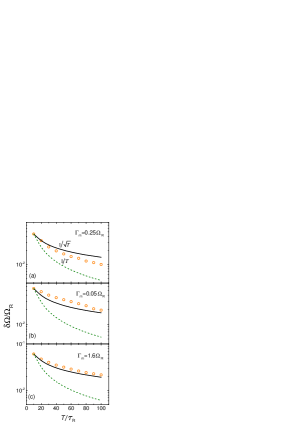
Figure 3: Estimate precision (root-mean-square variance) versus the measurement time (scaled by the Rabi period $\tau_{R}$). In particular, we compare the simulated results (open circles) with the SQL ($\sim 1/\sqrt{T}$, solid line) and HL ($\sim 1/T$, dashed line) scaling behaviors. In (a), by properly choosing the measurement strength (near the optimal one), we find that the precision can evidently exceed the SQL. In (b) and (c), we show that for measurement strengths deviating from the optimal/sub-optimal value, either the smaller or the larger values of $\Gamma_{m}$ cannot violate the SQL precision.

In quantum estimation, one of the most important problems is how the precision scales with the ‘size’ of the quantum resource (e.g. the entangled photon numbers in the optical phase estimation). For the quantum estimation based on continuous measurement (without introducing special procedures such as feedback), the existing studies assumed a SQL scaling ($\sim 1/\sqrt{T}$) with the measurement time $T$ Molm13 ; Molm14 ; Molm15 ; Molm16 ; Jor17 . Below we reexamine this issue in the context of continuous measurement in circuit-QED. We find that, remarkably, it is possible to violate the SQL.

Let us formally denote the RMS variance as $\delta\Omega=\frac{1}{\sqrt{M}}f(T)$, where the specific $M$ dependence is simply from the central-limit-theorem. Our interest is to examine the $T$ dependence, especially, to compare it with the SQL and HL scalings. As a clear comparison, in Fig. 3 we compare the simulated RMS variance with the SQL $C_{1}/\sqrt{T}$ (solid line) and HL $C_{2}/T$ (dashed line). Here we set the constants $C_{1}$ and $C_{2}$ by making the SQL and HL curves coincide with the simulated RMS variance at $T=10$. The two curves simply imply that, if the scaling is governed by SQL (HL), the simulated results should follow the solid (dashed) curve with increasing $T$.

In Fig. 3, we show results for different measurement strengths. Remarkably, as seen in Fig. 3(a), we find that by properly choosing the measurement strength (near the optimal one), the precision can evidently exceed the SQL. We notice that in the studies by Mølmer et al Molm13 ; Molm14 ; Molm15 ; Molm16 , only the $1/\sqrt{T}$ scaling is obtained for the Fisher information associated with the homodyne detection for the fluorescence radiation. This result was qualitatively understood by the measurement backaction which results in vanished correlation between the output signals. In the work by Jordan et al Jor17 , the $1/\sqrt{T}$ scaling is also briefly mentioned, despite that the $T$ scaling plotted there in Fig. 2(c) is a bit worse than SQL. In Appendix A, we further support the scaling behavior in Fig. 3(a) by numerically computing the Fisher information.

We may understand the result in Fig. 3(a) from different perspectives as follows. First, the ‘inconsistency’ with Refs. Molm13 ; Molm14 ; Molm15 ; Molm16 may originate from the different schemes of measurement. There, the measurement operator $\sigma_{\varphi}=\cos\varphi\sigma_{x}-\sin\varphi\sigma_{y}$ has randomly flipping backaction on the qubit. Compared to $\sigma_{z}$ measurement, this type of measurement has stronger destructive influence on the qubit, i.e., making the population (superposition) less associated with the Rabi frequency.

Second, for the continuous $\sigma_{z}$ measurement of the Rabi oscillation, quantum correlation exists between the measurement outcomes. Actually, this type of quantum correlation has inspired the study of the Bell-inequality-in-time, say, the Leggett-Garg inequality Leg85 . In particular, this quantum correlation has been experimentally demonstrated in the circuit-QED system based on the continuous $\sigma_{z}$ measurement Pala10 . Therefore, it seems that the argument of vanished correlation in Refs. Molm13 ; Molm14 ; Molm15 ; Molm16 , leading to the $1/\sqrt{T}$ scaling, may not apply to our situation.

Third, for the simple estimation scheme based on continuous measurement (not involving any special techniques), the possibility of reaching the Heisenberg limit is not ruled out (i) For instance, at the end of Ref. Molm14 , it was pointed out that the Fisher information can scale with $T^{2}$ for undamped system evolution, such as the case if the system superposition state does not couple to environment and the measurement is performed on the system rather than on the emitted radiation. (ii) In Ref. Gut11 , via analyzing the quantum Markov chain defined by a sequence of successive passage of atoms through a cavity, it was found that the quantum Fisher information scales quadratically rather than linearly with the number of atoms, at the limit of weak unitary interaction. (iii) Another example of interest is making the system (e.g., a driven atom under photon emissions) approach a dynamical phase transition Gar13 ; Gar16 . In that case, the quantum Fisher information may become quadratic in times shorter than the correlation time of the dynamics. This becomes valid for all times at the point of dynamical phase transition.

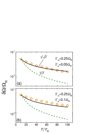
Figure 4: Further examination of the result in Fig. 3(a). Setting still the sub-optimal measurement strength $\Gamma_{m}=0.25\Omega_{R}$ but introducing extra decoherence ($\Gamma_{\varphi}$) owing to photon loss and/or amplifier’s noise during the measurement, we find that the result can no longer exceed the SQL precision. This supports further the understanding based on quantum correlation to the remarkable result in Fig. 3(a)

Therefore, our result in Fig. 3(a) does not contradict any basic physics, but rather can fall into the category of quantum correlation. As a trade-off between information gain and measurement backaction, a proper strength of the continuous measurement is required: As seen in Fig. 3(b) and (c), values deviating from the optimal/sub-optimal measurement strength, whether for smaller or larger values of $\Gamma_{m}$, will not lead to a violation of the SQL precision. In addition to the proper measurement strength, sufficient quantum coherence is another condition for the result in Fig. 3(a). In Fig. 4, we further account for the effect of decoherence owing to non-ideal quantum measurement, e.g., photon loss and/or amplifier’s noise during the measurement. From Fig. 4(a) and (b), we observe that the estimate precision becomes worse with the increase of decoherence, and can no longer violate the scaling of SQL by varying the measurement strength. This supports further our quantum-correlation-based understanding to the result in Fig. 3(a), since decoherence indeed suppresses the quantum correlation, as shown in Fig. 4.

V Summary and Discussions

We have reexamined the problem of quantum estimation of the Rabi frequency of qubit oscillations based on continuous measurement. We specified our research to the superconducting circuit-QED system which may provide an attractive platform for experimental examination. Our central result is that, by proper design of the measurement strength, the estimate precision can scale with the measurement time beyond the standard quantum limit. We understood this result by quantum correlation between the output signals which is supported by checking the effect of quantum efficiency of the measurement. Our conclusion is also supported by the scaling behavior of the associated Fisher information, as shown in Appendix A. We expect this preliminary result to inspire further studies on this interesting problem, including searching for better schemes of continuous measurement and special techniques such as feedback and quantum smoothing.

As a final remark, we mention again that the present work is an extension of the previous studies on the quantum estimation of parameters by continuous measurements Jac11 ; Molm13 ; Molm14 ; Molm15 ; Molm16 ; Jor17 ; Par17 ; Gen17 . In particular, the effective measurement operator ($\sigma_{z}$) for the Rabi oscillation is essentially the same as considered in Ref. Jor17 , where the main interest was focused on accelerating the likelihood-estimation method and the estimation of drifting parameters. This focus may have caused an overlook of the $T$ (measurement time) scaling behavior of the estimate precision. Probably affected by the $1/\sqrt{T}$ scaling concluded by Mølmer et al Molm13 ; Molm14 ; Molm15 ; Molm16 , this scaling was also briefly mentioned in Ref. Jor17 below Eq. (16) associated with Fig. 2(c) (despite that the result in Fig. 2(c) is a bit worse than the $1/\sqrt{T}$ scaling). This difference, compared to our Fig. 3(a), may originate from not finding a proper measurement strength and simulating fewer number of trajectories there. As a further support, in Appendix A we include the result of our simulated Fisher information and find similar scaling behavior beyond the SQL, being consistent with that shown in Fig. 3(a).

Another point is that the measurement time we simulated may be not long enough to reach the asymptotic behavior. However, the scaling behavior even for this ‘intermediate’ regime is relevant in practical sense to the estimation problem under study. We notice that the scaling behavior even for relatively short time has been considered with interest. For instance, in Refs. Gar13 ; Gar16 , it was found that the quantum Fisher information can become quadratic in times shorter than the correlation time of the dynamics.

Acknowledgements.

— This work was supported by the National Key Research and Development Program of China (No. 2017YFA0303304) and the NNSF of China (No. 11675016).

Appendix A Scaling Behavior of the Fisher Information

In this Appendix, we carry out the Fisher information associated with the present continuous measurement scheme. The Fisher information is given by

$${\cal F}_{T}(\Omega)=\int dx\,{\cal P}(x|\Omega)\left(\frac{\partial\ln{\cal P}(x|\Omega)}{\partial\Omega}\right)^{2}\,.$$ (11)

Here the short hand notation $x=\{{\cal I}_{1},{\cal I}_{1},\cdots,{\cal I}_{N}\}$ is introduced for simplicity, and the integration is in principle over all the possible output currents from measurement realizations over time $T$.

In practice, we compute the Fisher information by numerically averaging 20000 trajectories (realizations). For each trajectory, we compute the derivative $\partial\ln{\cal P}/\partial\Omega$ from the likelihood function at the real value $\Omega$. In Fig. 5 we show the result of Fisher information against the measurement time $T$, for the measurement strength $\Gamma_{m}/\Omega_{R}=0.25$ corresponding to Fig. 3(a). In particular, in Fig. 5(b) we compare the result with the scaling behaviors of the RMS variance $\delta\Omega$ and the SQL. As in the plots of Figs. 3 and 4 in the main text, here we plot $\sim 1/\sqrt{{\cal F}_{T}}$ by equating it with the simulated RMS variance $\delta\Omega$ at the starting point. Then, from this type of plotting and if we assume ${\cal F}_{T}\sim T^{n}$, we can deduce the scaling index $n>1$, which exceeds the SQL scaling. Moreover, in Fig. 5(b), we find satisfactory agreement between the $T$ scalings of the Fisher information and the RMS variance $\delta\Omega$. This supports further the conclusion we achieved in the main text.

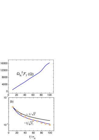
Figure 5: Scaling behavior of the Fisher information ${\cal F}_{T}(\Omega)$ against the measurement time $T$, for measurement strength $\Gamma_{m}/\Omega_{R}=0.25$ corresponding to Fig. 3(a). Particularly, in (b) we compare the time scaling of the Fisher information (blue curve) with the SQL (black curve) and the RMS variance $\delta\Omega$ (orange circles, taken from Fig. 3(a)).

References

- (1) C. W. Helstrom,J. Stat. Phys. 1, 231 (1969).
- (2) A. S. Holevo, Probabilistic and Statistical Aspects of Quantum Theory (Springer Science & Business Media, New York, 2011), Vol. 1.
- (3) V. Giovannetti, S. Lloyd, and L. Maccone, Science 306, 1330 (2004).
- (4) V. Giovannetti, S. Lloyd and L. Maccone, Nat. Photon. 5, 222 (2011).
- (5) R. Demkowicz-Dobrzanski, M. Jarzyna and J. Kolodynski, Prog. Opt. 60, 345 (2015).
- (6) D. J. Wineland, J. J. Bollinger, W. M. Itano, F. L. Moore and D. J. Heinzen, Phys. Rev. A 46, R6797 (1992).
- (7) J. J. Bollinger, W. M. Itano, D. J. Wineland and D. J. Heinzen, Phys. Rev. A 54, R4649 (1996).
- (8) C. W. Helstrom, Quantum Detection and Estimation Theory (Academic Press, New York, 1976).
- (9) S. L. Braunstein and C. M. Caves, Phys. Rev. Lett. 72, 3439 (1994).
- (10) H. Cramér, Mathematical Methods of Statistics (Princeton University Press, Princeton, NJ, 1946).
- (11) C. R. Rao, Bull. Calcutta Math. Soc. 37, 81 (1945).
- (12) J. F. Ralph, K. Jacobs, and C. D. Hill, Phys. Rev. A 84, 052119 (2011).
- (13) S. Gammelmark and K. Mølmer, Phys. Rev. A 87, 032115 (2013).
- (14) S. Gammelmark and K. Mølmer, Phys. Rev. Lett. 112, 170401 (2014).
- (15) A. H. Kiilerich and K. Mølmer, Phys. Rev. A 92, 032124 (2015).
- (16) A. H. Kiilerich and K. Mølmer, Phys. Rev. A 94, 032103 (2016).
- (17) L. Cortez, A. Chantasri, L. P. García-Pintos, J. Dressel, and A. N. Jordan, Phys. Rev. A 95, 012314 (2017).
- (18) F. Albarelli, M. A. C. Rossi, M. G. A. Paris, and M. G. Genoni, New J. Phys. 19, 123011 (2017).
- (19) M. G. Genoni, Phys. Rev. A 95, 012116 (2017).
- (20) M. Tsang, Phys. Rev. Lett. 102, 250403 (2009).
- (21) M. Tsang, Phys. Rev. A 80, 033840 (2009).
- (22) M. Tsang, Phys. Rev. A 81, 013824 (2010).
- (23) M. Tsang, Phys. Rev. A 92, 062119 (2015).
- (24) A. Blais, R. S. Huang, A. Wallraff, S. M. Girvin, and R. J. Schoelkopf, Phys. Rev. A 69, 062320 (2004).
- (25) A. Wallraff, D. I. Schuster, A. Blais, L. Frunzio, R. S. Huang, J. Majer, S. Kumar, S. M. Girvin, and R. J. Schoelkopf, Nature (London) 431, 162 (2004).
- (26) R. J. Schoelkopf, and S. M. Girvin, Nature (London) 451, 664 (2008).
- (27) J. P. Groen, D. Risté, L. Tornberg, J. Cramer, P. C. de Groot, T. Picot, G. Johansson, and L. DiCarlo, Phys. Rev. Lett. 111, 090506 (2013).
- (28) P. Campagne-Ibarcq, E. Flurin, N. Roch, D. Darson, P. Morfin, M. Mirrahimi, M. H. Devoret, F. Mallet, and B. Huard, Phys. Rev. X 3, 021008 (2013).
- (29) M. Hatridge, S. Shankar, M. Mirrahimi, F. Schackert, K. Geerlings, T. Brecht, K. M. Sliwa, B. Abdo, L. Frunzio, S. M. Girvin, R. J. Schoelkopf, and M. H. Devoret, Science 339, 178 (2013).
- (30) K. W. Murch, S. J. Weber, C. Macklin, and I. Siddiqi, Nature (London) 502, 211 (2013).
- (31) D. Tan, S. J. Weber, I. Siddiqi, K. Molmer, and K. W. Murch, Phys. Rev. Lett. 114, 090403 (2015).
- (32) R. Vijay, C. Macklin, D. H. Slichter, S. J. Weber, K. W. Murch, R. Naik, A. N. Korotkov, and I. Siddiqi, Nature (London) 490, 77 (2012).
- (33) A. N. Korotkov, arXiv:1111.4016; see also chapter 17 in Les Houches 2011 session XCVI on Quantum Machines.
- (34) A. N. Korotkov, Phys. Rev. A 94, 042326 (2016).
- (35) P. Y. Wang, L. P. Qin, and X.-Q. Li, New J. Phys. 16, 123047 (2014); ibid. 17, 059501 (2015).
- (36) W. Feng, P. F. Liang, L. P. Qin, and X.-Q. Li, Sci. Rep. 6, 20492 (2016).
- (37) W. Feng, C. Zhang, Z. Wang, L. Qin, and X.-Q. Li, Phys. Rev. A 98, 022121 (2018).
- (38) J. Gambetta, A. Blais, M. Boissonneault, A. A. Houck, D. I. Schuster, and S. M. Girvin, Phys. Rev. A 77, 012112 (2008).
- (39) H. M. Wiseman and G. J. Milburn, Quantum Measurement and Control (Cambridge Univ. Press, Cambridge, 2009).
- (40) K. Jacobs, Quantum Measurement Theory and Its Applications (Cambridge Univ. Press, Cambridge, 2014).
- (41) A. J. Leggett and A. Garg, Phys. Rev. Lett. 54, 857 (1985).
- (42) A. Palacios-Laloy, F. Mallet, F. Nguyen, P. Bertet, D. Vion, D. Esteve, and A. N. Korotkov, Nat. Phys. 6, 442 (2010).
- (43) M. Guta, Phys. Rev. A 83, 062324 (2011).
- (44) I. Lesanovsky, M. van Horssen, M. Gutua, and J. P. Garrahan, Phys. Rev. Lett. 110, 150401 (2013).
- (45) K. Macieszczak, M. Guta, I. Lesanovsky, and J. P. Garrahan, Phys. Rev. A 93, 022103 (2016).