Duistermaat-Heckman measure and the mixture of quantum states

Abstract

In this paper, we present a general framework to solve a fundamental problem in Random Matrix Theory (RMT), i.e., the problem of describing the joint distribution of eigenvalues of the sum $\boldsymbol{A}+\boldsymbol{B}$ of two independent random Hermitian matrices $\boldsymbol{A}$ and $\boldsymbol{B}$. Some considerations about the mixture of quantum states are basically subsumed into the above mathematical problem. Instead, we focus on deriving the spectral density of the mixture of adjoint orbits of quantum states in terms of Duistermaat-Heckman measure, originated from the theory of symplectic geometry. Based on this method, we can obtain the spectral density of the mixture of independent random states. In particular, we obtain explicit formulas for the mixture of random qubits. We also find that, in the two-level quantum system, the average entropy of the equiprobable mixture of $n$ random density matrices chosen from a random state ensemble (specified in the text) increases with the number $n$. Hence, as a physical application, our results quantitatively explain that the quantum coherence of the mixture monotonously decreases statistically as the number of components $n$ in the mixture. Besides, our method may be used to investigate some statistical properties of a special subclass of unital qubit channels.
 
Mathematics Subject Classification. 22E70, 81Q10, 46L30, 15A90, 81R05
Keywords. Duistermaat-Heckman measure; Horn’s problem; probability density function; quantum coherence

1 Introduction

According to one of postulates in Quantum Mechanics, the pure state of a single quantum system is represented by a vector in a complex Hilbert space. It is also well-known that Hilbert space of a composite quantum system is characterized by the tensor product of the Hilbert spaces of the individual components. Clearly the dimension of a composite quantum system grows exponentially with the number of their components. This leads to exponential complexity. Recently, Christandl et al in [8] had presented an effective method in order to get some physical features which depend only on the eigenvalues of the one-body reduced states of a randomly-chosen multipartite quantum state. Let us briefly recall their work here. In more detail, they have described an explicit algorithm to compute the joint eigenvalue distribution of all the reduced density matrices of a pure multipartite quantum state drawn at random from the unitarily invariant distribution. Moreover, the situation for the mixed state can always be reduced to the pure state case by the purification technique. Mathematically, the eigenvalue distributions obtained are just Duistermaat-Heckman measures on the moment polytope [11]. Here the moment polytope [6], i.e., the support of Duistermaat-Heckman measure, is the solution of the one-body quantum marginal problem, i.e., the problem of identifying the set of possible reduced density matrices; the Duistermaat-Heckman measure is defined to be the push-forward of the Liouville measure on a symplectic manifold along a moment map. Later, some specific examples (lower dimensional computation) are given based on their algorithm solution to the one-body quantum marginal problem. In particular, some eigenvalue distributions involved in qubits can be explicitly illustrated. As noted by the authors, the well-known Horn’s problem [14], i.e., the determination of the possible eigenvalues of the sum of two Hermitian matrices with fixed eigenvalues, is a specific application of the one-body quantum marginal problem. Moreover, they used their approach to easily recover the main result, that is, (2.5), obtained in [10]. But, however, they just obtained only abstract formula (2.5) with no explicit expressions and without applying it to study random states in quantum information theory. In fact, the (probabilistic) mixture (i.e., the convex combination) of quantum states is necessarily encountered in quantum information theory. For example, the mixture of quantum states arises in the convexity of the entanglement measure and the coherence measure, etc. Thus, it is necessary to figure out the spectral density of the mixture when we use the technique of Random Matrix Theory (RMT) [27] to study relevant problems. Motivated by this, in the paper, we will focus on Duistermaat-Heckman measure over the moment polytope corresponding to the Horn’s problem and provide some analytical computations in lower dimensional spaces which are perhaps related to some problems in quantum information theory. Another motivation about this investigation is perhaps related to the well-known fact—the distribution law of the sum of independent random variables is described by the convolution of the distribution law of individual random variables—in Probability Theory. Instead, what we will consider in the paper is to describe the spectral law of the sum of non-commutative random variables, i.e., random Hermitian matrices. In particular, we focus on the distribution law of the mixture of random quantum states. The framework introduced in the work can just applies to such problem.

To be more specific, we consider the following problem: To derive the spectral density of the equiprobable mixture of $n$ random density matrices (i.e., positive semi-definite complex matrix of unit trace), each of them chosen from an adjoint orbit $\mathcal{O}_{\rho}$. Here the adjoint orbit $\mathcal{O}_{\rho}$ of $\rho$ is the set of isospectral density matrices, that is, $\mathcal{O}_{\rho}=\left\{\boldsymbol{U}\rho\boldsymbol{U}^{\dagger}:\boldsymbol{U}\in\mathrm{S}\mathrm{U}(d)\right\}$, where $\mathrm{S}\mathrm{U}(d)$ is the special unitary group of $d\times d$ unitary complex matrices. Apparently, $\mathcal{O}_{\rho}$ is essentially determined by the spectrum of $\rho$. If we write $\boldsymbol{\lambda}=(\lambda_{1},\ldots,\lambda_{d})$ for the spectrum of $\rho$, i.e., a probability vector with $\lambda_{1}\geqslant\cdots\geqslant\lambda_{d}\geqslant 0$ and $\sum^{d}_{j=1}\lambda_{j}=1$, then $\mathcal{O}_{\rho}=\mathcal{O}_{\boldsymbol{\lambda}}$. With the above notations, our problem can be reformulated as: Given $n$ probability vectors $\boldsymbol{\lambda}^{1},\ldots,\boldsymbol{\lambda}^{n}$, we derive the spectral density of the mixture:

$$\rho_{s}=\frac{1}{n}\left(\sum^{n}_{j=1}\boldsymbol{U}_{j}\boldsymbol{\lambda}^{j}\boldsymbol{U}^{\dagger}_{j}\right),$$ (1.1)

where each $\boldsymbol{U}_{j}\in\mathrm{S}\mathrm{U}(d)$ distributed according to the normalized Haar measure. Note here that we make abuse of notations: all $\boldsymbol{\lambda}^{j}$ can be viewed as diagonal matrices $\mathrm{diag}\left(\lambda^{(j)}_{1},\ldots,\lambda^{(j)}_{d}\right)$, or vectors $\left(\lambda^{(j)}_{1},\ldots,\lambda^{(j)}_{d}\right)$ according to the context. Interestingly, if all $\boldsymbol{\lambda}^{j}$ are equal to the same $\boldsymbol{\lambda}$, then (1.1) can be viewed as a image of a random mixed-unitary channel $\Phi$: $\rho_{s}=\Phi(\boldsymbol{\lambda})$.

Once we work out the spectral density of (1.1), we can use this to derive the spectral density of the equiprobable mixture:

$$\rho=\frac{1}{n}\sum^{n}_{j=1}\rho_{j},$$ (1.2)

where $\rho_{j}\in\mathrm{D}\left(\mathbb{C}^{d}\right)$, the set of all $d\times d$ density matrices, for $j=1,\ldots,n$ are chosen independently from the following random state ensemble $\mathcal{E}_{d,k}(d\leqslant k)$ which are explained immediately. Such ensemble $\mathcal{E}_{d,k}$ is obtained by partial-tracing over the $k$-dimensional subsystem of a $dk$-dimensional composite quantum system in pure states which are Haar-distributed. Because we have already known the eigenvalue distribution of the ensemble $\mathcal{E}_{d,k}$ [36], i.e.,

$$p_{d,k}(\boldsymbol{\lambda}):=p_{d,k}(\lambda_{1},\ldots,\lambda_{d})=C_{d,k}\delta\left(1-\sum^{d}_{j=1}\lambda_{j}\right)\prod^{d}_{j=1}\lambda^{k-d}_{j}\theta(\lambda_{j})\prod_{1\leqslant i<j\leqslant d}(\lambda_{i}-\lambda_{j})^{2}.$$ (1.3)

The notations above are explained as follows. Here $C_{d,k}$ is the normalization constant, given by

$$C_{d,k}=\frac{\Gamma(dk)}{\prod^{d-1}_{j=0}\Gamma(k-j)\Gamma(d-j+1)}.$$

Note that $\Gamma(z)$ is the Gamma function, defined for all complex number with positive real part: $\Gamma(z)=\int^{\infty}_{0}x^{z-1}e^{-x}\mathrm{d}x$. In addition, $\delta$ is the Dirac delta function [15]. Besides, $\theta(x)$ is a function defined by $\theta(x)=1$ if $x>0$; otherwise, $\theta(x)=0$. Now we can answer the question (1.2) based on the solution to (1.1). In fact, denote the spectral density of $\rho_{s}$ by $p\left(\boldsymbol{\lambda}^{s}|\boldsymbol{\lambda}^{1},\ldots,\boldsymbol{\lambda}^{n}\right)$, we conclude that the spectral density of $\rho$ in (1.2) is given by the following multiple integral:

$$\int p\left(\boldsymbol{\lambda}^{s}|\boldsymbol{\lambda}^{1},\ldots,\boldsymbol{\lambda}^{n}\right)\prod^{n}_{j=1}p_{d,k}\left(\boldsymbol{\lambda}^{j}\right)\left[\mathrm{d}\boldsymbol{\lambda}^{j}\right],$$

where the function $p_{d,k}$ is from (1.3) and $\left[\mathrm{d}\boldsymbol{\lambda}^{j}\right]$ is the Lebesgue volume element in $\mathbb{R}^{d}$, defined by $\left[\mathrm{d}\boldsymbol{\lambda}^{j}\right]=\prod^{d}_{i=1}\mathrm{d}\lambda^{(j)}_{i}$.

In view of this, let us focus on the derivation of the spectral density of (1.1). Before proceeding, some remarks are necessary. Basically, what we are considered in the paper are intimately related to Horn’s problem (also called Horn’s conjecture), as mentioned previously. The Horn’s problem asks for the spectrum of eigenvalues of the sum of two given Hermitian matrices with fixed eigenvalues. Specifically, given two Hermitian matrices $\boldsymbol{A}$ and $\boldsymbol{B}$ with respective spectra $\boldsymbol{a}$ and $\boldsymbol{b}$, the goal of Horn’s problem is to identify the spectrum of $\boldsymbol{A}+\boldsymbol{B}$. The solutions of Horn’s problem, as vectors, form a convex polytope whose describing linear inequalities have been conjectured by Horn in 1962 [14]. Although this problem has already completely solved by Klyachko [18] and also by Knutson and Tao [20, 21], later several other proofs were presented, for instance, [1]. Such convex polytope are often defined by an exponential number of linear inequalities when the matrix size are large enough. The general problem is computationally intractable, it is also NP-hard. This motivates us to get explicit computations for some small matrix sizes. What we contributed in this paper is to derive explicit expressions for the eigenvalue distribution of the sum of several matrices (say, two or more) instead of the determination of the possible eigenvalues of the sum. Furthermore, these matrices are restricted to be proportional to density matrices. Note that the matrix size are restricted to no more than four in the paper since analytical computation for matrix sizes larger than four seems too complicated to be practical. In view of this reason, our method provide a complete solution to the above problem algorithmically in higher dimension.

We also consider the derivation of the probability density of the diagonal part of $\rho_{s}$, defined in (1.1). Let us recall some notions related to it and its generalizations. A well-known result of Isaac Schur [28] indicates that the diagonal elements $(a_{11},\ldots,a_{dd})$ of a $d\times d$ Hermitian matrix $\boldsymbol{A}=(a_{ij})$ solves a system of linear inequalities involving the eigenvalues $(\lambda_{1},\ldots,\lambda_{d})$. Indeed, if we viewing $\boldsymbol{a}=(a_{11},\ldots,a_{dd})^{\scriptscriptstyle\mathsf{T}}$ and $\boldsymbol{\lambda}=(\lambda_{1},\ldots,\lambda_{d})^{\scriptscriptstyle\mathsf{T}}$ as points in $\mathbb{R}^{d}$, then by the Spectral Decomposition Theorem of a Hermitian matrix, there exists a special unitary $\boldsymbol{U}\in\mathrm{S}\mathrm{U}(d)$ such that $\boldsymbol{A}=\boldsymbol{U}\boldsymbol{\lambda}\boldsymbol{U}^{\dagger}$. Then $\boldsymbol{a}=(\boldsymbol{U}\star\overline{\boldsymbol{U}})\boldsymbol{\lambda}$, where $\star$ stands for the Schur product for both matrices with the same size, and the bar means to taking the complex conjugate entrywise. That is, $\boldsymbol{A}\star\boldsymbol{B}=(a_{ij}b_{ij})$. Clearly $\boldsymbol{U}\star\overline{\boldsymbol{U}}$ is a $d\times d$ unistochastic matrix, a fortiori bi-stochastic matrix (with nonnegative entries, and both column-sum and row-sum being equal to one). By Birkhoff-von Neumann theorem [29], we have obtained that $\boldsymbol{a}$ is in the convex hull of the points $S_{d}\cdot\boldsymbol{\lambda}$. Here the action of $S_{d}$ on the vector $\boldsymbol{\lambda}$ by permutating its coordinates. Later, A. Horn shown [13] the converse to the above result holds true. Thus this convex hull is exactly the set of diagonal parts of all elements from $\mathcal{O}_{\boldsymbol{\lambda}}$. A more general result related to Horn’s result is obtained by B. Kostant [22]. It is easily seen from (1.1) that the diagonal part (as a column vector) of $\rho_{s}$ in (1.1) is determined by

$$\rho^{D}_{s}=\frac{1}{n}\sum^{n}_{j=1}(\boldsymbol{U}_{j}\star\overline{\boldsymbol{U}}_{j})\boldsymbol{\lambda}^{j}.$$

The second goal of this paper is to identify the probability density of $\rho^{D}_{s}$ in (1.1) when all $\boldsymbol{\lambda}^{j}$ are fixed and $\boldsymbol{U}_{j}$ are Haar-distributed.

The probability densities of the diagonal part and eigenvalues of the mixture of several random qubits can be used to infer the distribution of von Neumann entropy. As an application in quantum information theory, we use our results to compute the average entropy of the mixture of random quantum states and that of its corresponding diagonal part. Furthermore, these computations can be used to explain that the quantum coherence [2] of the mixture decreases statistically as the number of components in the mixture of qubits, as already noted in [30, 33]. In this process, we shall see that the relative entropy of coherence, one of kinds of many quantum coherence measures, defined via the relative entropy, naturally relates the diagonal part and eigenvalues of a quantum state.

The paper is organized as follows. In Section 2, we present background tools related to this paper, and recall the results obtained in [10] by formulation used in [8]. Then, we consider the equiprobable mixture of several qubit states, i.e., we derive the spectral density of two qubit states and three qubit states (Theorem 3.4–Theorem 3.7), respectively, in Section 3. Moreover, we present two examples to demonstrate our method: In the first example, i.e., Example 3.11, the density function of eigenvalues of the equiprobable mixture of two qutrits with given spectra is identified analytically; in the second example, i.e., Example 3.15, we derive the density function of eigenvalues of the equiprobable mixture of two two-qubits with given spectra over some subregion of the support. Sequentially, in Section 4, we present an application of our results in quantum information theory. That is, the quantum coherence of the mixture monotonously decreases statistically as the number of components $n$. We conclude the paper with summary in Section 5.

2 Preliminaries

As we shall see, Duistermaat-Heckman measure [11] is our central tool in the paper. In preparation for defining Duistermaat-Heckman measure, we need to make an introduction about push-forward measure or image measure from measure theory [4]. After that, we give the formal definition of the moment map for a symplectic manifold [25]. Finally, we focus on the product of coadjoint orbits where our problems will be investigated. Note that we collect some notions (not new) together in the section in order for the paper to be self-contained.

2.1 Push-forward measure

In measure theory, a push-forward measure is obtained by transferring a measure from one measurable space to another using a measurable function. The following definition and fact about push-forward measure can be found in [4].

Definition 2.1 (Push-forward of a measure).

Given two measurable spaces $(\mathcal{X},\mathcal{F})$ and $(\mathcal{Y},\mathcal{G})$, a measurable mapping $\Phi:\mathcal{X}\to\mathcal{Y}$ and a measure $\mu:\mathcal{F}\to[0,+\infty]$, the push-forward of $\mu$ is defined to be the measure $\Phi_{*}\mu:\mathcal{G}\to[0,+\infty]$ given by

$$(\Phi_{*}\mu)(B)=\mu\left(\Phi^{-1}(B)\right)\quad\text{for}\quad B\in\mathcal{G}.$$

The following result about the push-forward measure will be used in the paper.

Proposition 2.2 (Change of variables formula).

Given two measurable spaces $(\mathcal{X},\mathcal{F})$ and $(\mathcal{Y},\mathcal{G})$, a measurable mapping $\Phi:\mathcal{X}\to\mathcal{Y}$ and a measure $\mu:\mathcal{F}\to[0,+\infty]$. A measurable function $f$ on $\mathcal{Y}$ is integrable with respect to the push-forward measure $\Phi_{*}\mu$ if and only if the composition $\Phi\circ f$ is integrable with respect to the measure $\mu$. In that case, the integrals coincide:

$$\int_{\mathcal{Y}}f\mathrm{d}(\Phi_{*}\mu)=\int_{\mathcal{X}}f\circ\Phi\mathrm{d}\mu:=\int_{\mathcal{X}}(\Phi^{*}f)\mathrm{d}\mu,$$

where $\Phi^{*}f:=f\circ\Phi$ is the function on $\mathcal{X}$, called the pull-back of the function $f$ on $\mathcal{Y}$. In the notation of distribution, the above fact can be represented by

$$\left\langle\Phi_{*}\mu,f\right\rangle=\left\langle\mu,\Phi^{*}f\right\rangle.$$

Here $\left\langle\cdot,\cdot\right\rangle$ denotes the pairing between measures and test functions.

With this notion, we can describe the main notions used in the paper.

2.2 Moment map

The notions mentioned in this part can be found in [24, 17].

Definition 2.3 (Symplectic manifold).

Assume that $M$ is a smooth manifold. $M$ is called symplectic manifold if there exists a closed non-degenerate 2-form $\omega_{M}$ on $M$. That is,

1. $\omega_{M}$ is a 2-form: It is a anti-symmetric and bilinear form on the product of two tangent spaces $\textsf{T}_{m}M\times\textsf{T}_{m}M$ for each $m\in M$;

2. $\omega_{M}$ is closed: $\mathrm{d}\omega_{M}=0$;

3. $\omega_{M}$ is non-degenerate: on each tangent space $\textsf{T}_{m}M(m\in M)$: if $\omega_{M}(\xi,\eta)=0$ for all $\eta\in\textsf{T}_{m}M$, then $\xi=0$.

Note that a closed non-degenerate 2-form is called symplectic form.

Definition 2.4 (Action of a Lie group on a manifold).

Let $M$ be a smooth manifold. An action of a Lie group $G$ on $M$ is a smooth mapping $\tau:G\times M\to M$, such that

1. for all $m\in M$, $\tau(e,m)=m$ and

2. for every $g,h\in G$, $\tau(g,\tau(h,m))=\tau(gh,m)$ for all $m\in M$.

For every $g\in G$, let $\tau_{g}:M\to M$ be given via $m\mapsto\tau_{g}(m)$. The above definition can be rephrased as: the mapping $g\mapsto\tau_{g}$ is a homomorphism of $G$ into the group of diffeomorphisms of $M$. If $M$ is a vector space and each $\tau_{g}$ is a linear transformation, the action of $G$ on $M$ is called a representation of $G$ on $M$.

Suppose $\tau:G\times M\to M$ is a smooth action. If $\xi\in\mathfrak{g}$, the Lie algebra of $G$, then $\tau^{\xi}:\mathbb{R}\times M\to M$ is given via $(t,\xi)\mapsto\tau(e^{t\xi},m)$ is an $\mathbb{R}$-action on $M$, that is, $\tau^{\xi}$ is a flow on $M$. The corresponding vector field on $M$ is given by $\xi_{M}(m):=\left.\frac{\mathrm{d}}{\mathrm{d}t}\right|_{t=0}\tau_{e^{t\xi}}(m)$ is called the infinitesimal generator of the action corresponding to $\xi$.

The adjoint representation $\mathrm{Ad}$ of $G$ on its Lie algebra $\mathfrak{g}$ is given by

$$G\times\mathfrak{g}\to\mathfrak{g},\quad(g,\xi)\mapsto g\cdot\xi:=\mathrm{Ad}(g)\xi=g\xi g^{-1}.$$

This adjoint representation of $G$ on $\mathfrak{g}$ induces a coadjoint representation $\mathrm{Ad}^{*}$ of $G$ on $\mathfrak{g}^{*}$ (the dual space of $\mathfrak{g}$):

$$G\times\mathfrak{g}^{*}\to\mathfrak{g}^{*},\quad(g,\varphi)\mapsto g\cdot\varphi=\mathrm{Ad}^{*}(g)\varphi=\mathrm{Ad}(g^{-1})^{*}\varphi,$$

where $\left\langle\mathrm{Ad}(g^{-1})^{*}\varphi,\eta\right\rangle=\left\langle\varphi,\mathrm{Ad}(g^{-1})\eta\right\rangle$. That is, $\mathrm{Ad}(g^{-1})^{*}\varphi$ is the pull-back of $\varphi$ under the mapping $\mathrm{Ad}(g^{-1})$.

Definition 2.5 (Moment map).

Let $(M,\omega_{M})$ be a connected symplectic manifold and $\tau:G\times M\to M$ a symplectic action of the Lie group $G$ on $M$; that is, for each $g\in G$, the map $\tau_{g}:M\to M$ is given via $\tau_{g}(m)=\tau(g,m)$ is symplectic, i.e., $\tau^{*}_{g}\omega_{M}=\omega_{M}$. We say that a mapping $\Phi_{G}:M\to\mathfrak{g}^{*}$ is a moment map for the action if, for every $\xi\in\mathfrak{g}$,

$$\mathrm{d}\phi^{\xi}=\omega_{M}(\xi_{M},\cdot):=\iota(\xi_{M})\omega_{M},$$ (2.1)

where $\left\langle\Phi_{G},\xi\right\rangle=\phi^{\xi}:M\to\mathbb{R}$ is defined by $\phi^{\xi}(m):=\left\langle\Phi_{G}(m),\xi\right\rangle$, and $\xi_{M}$ is the infinitesimal generator of the action corresponding to $\xi\in\mathfrak{g}$. Sometimes $(M,\omega_{M},G,\Phi_{G})$ is called a Hamiltonian $G$-manifold.

Example 2.6 (The symplectic structure of a co-adjoint orbit).

Let $G$ be a compact connected Lie group with its Lie algebra $\mathfrak{g}$. Assume that $G$ acts on $\mathfrak{g}$ by the adjoint action, and acts on $\mathfrak{g}^{*}$ by the co-adjoint action, as mentioned above. Fix $\lambda\in\mathfrak{g}^{*}$ and let $\mathcal{O}_{\lambda}=G\cdot\lambda$ by the co-adjoint action. The infinitesimal generator of the co-adjoint action of $G$, corresponding to $\xi\in\mathfrak{g}$, is given by $\xi_{\mathcal{O}_{\lambda}}(f)=-f\circ\mathrm{ad}(\xi),\quad f\in\mathcal{O}_{\lambda}$. The Kirillov-Kostant-Souriau 2-form on $\mathcal{O}_{\lambda}$ is defined by

$$\omega(\xi_{\mathcal{O}_{\lambda}}(f),\eta_{\mathcal{O}_{\lambda}}(f))=-f([\xi,\eta]),\quad f\in\mathcal{O}_{\lambda},\xi,\eta\in\mathfrak{g}.$$ (2.2)

Moreover $\omega$ is a well-defined smooth and closed non-degenerate 2-form on $\mathcal{O}_{\lambda}$ so that $(\mathcal{O}_{\lambda},\omega)$ is a symplectic manifold. Furthermore, $\omega$ is $G$-invariant, thus a symplectic form. The minus inclusion map $\Phi_{G}:\mathcal{O}_{\lambda}\hookrightarrow\mathfrak{g}^{*}$ is a moment map, i.e., $\Phi_{G}$ is $G$-equivariant and $\mathrm{d}\phi^{\xi}=\iota(\xi_{\mathcal{O}_{\lambda}})\omega\quad\xi\in\mathfrak{g}$, where $\phi^{\xi}=\left\langle\Phi_{G},\xi\right\rangle:\mathcal{O}_{\lambda}\to\mathbb{R}$. Note that adjoint orbits in $\mathfrak{g}$ can be identified with co-adjoint orbits in $\mathfrak{g}^{*}$ by choosing a positive definite $G$-invariant form on $\mathfrak{g}$. This convention will be used throughout in the paper.

2.3 Duistermaat-Heckman measure

Throughout the paper, $K$ will denote a compact, connected Lie group with maximal torus (maximal commutative subgroup) $T\subset K$, Weyl group (the normalizer of $T$) $W$, respective Lie algebras $\mathfrak{k},\mathfrak{t}$. We write $\pi_{K,T}:\mathfrak{k}^{*}\to\mathfrak{t}^{*}$ for the projection dual to the inclusion $\mathfrak{t}\subset\mathfrak{k}$. Here $\mathfrak{k}^{*}$ ($\mathfrak{t}^{*}$) means the dual space of $\mathfrak{k}$ ($\mathfrak{t}$). Let us also choose a positive Weyl chamber $\mathfrak{t}^{*}_{\geqslant 0}\subset\mathfrak{t}^{*}$; this determines a set of positive roots $\{\alpha_{1},\ldots,\alpha_{R}\}\subset\mathrm{i}\mathfrak{t}^{*}$. All positive roots are denoted simple by $\alpha>0$. We also denote by $\mathfrak{t}^{*}_{>0}$ the interior of the positive Weyl chamber. The notions related to theory of compact Lie groups and its Lie algebras can be found in [12].

Definition 2.7 (Duistermaat-Heckman measure).

Let $M$ be a compact, connected Hamiltonian $K$-manifold of dimension $2m$, with symplectic form $\omega_{M}$ (a closed non-degenerate 2-form) and a choice of moment map $\Phi_{K}:M\to\mathrm{i}\mathfrak{k}^{*}$, as in Definition 2.5. The Liouville measure on $M$ is defined by $\mu_{M}:=\frac{\omega^{\wedge m}_{M}}{(2\pi)^{m}m!}$, where $\omega^{\wedge m}_{M}=\overbrace{\omega_{M}\wedge\cdots\wedge\omega_{M}}^{m}$ is the $m$-th exterior power of $\omega_{M}$. More precisely, for a Borel subset $B$ of $M$, the Liouville measure of $B$ is given by $\mu_{M}(B)=\int_{B}\frac{\omega^{\wedge m}_{M}}{(2\pi)^{m}m!}$. The non-Abelian Duistermaat-Heckman measure $\mathrm{DH}^{K}_{M}$ is defined as follows:

$$\mathrm{DH}^{K}_{M}=\frac{1}{p_{K}}(\tau_{K})_{*}(\Phi_{K})_{*}(\mu_{M}),$$

where $\tau_{K}:\mathrm{i}\mathfrak{k}^{*}\to\mathrm{i}\mathfrak{t}^{*}_{\geqslant 0}$ is defined as $\tau_{K}(\mathcal{O}_{\lambda})=\lambda$ for $\lambda\in\mathrm{i}\mathfrak{t}^{*}_{\geqslant 0}$ and $p_{K}(\lambda)=\mathrm{vol}(\mathcal{O}_{\lambda})=\prod_{\alpha>0}\frac{\langle\lambda,\alpha\rangle}{\langle\alpha,\varpi\rangle}$ for $\varpi=\frac{1}{2}\sum_{\alpha>0}\alpha$, half the sum of all positive roots. Here $\mathrm{vol}(\mathcal{O}_{\lambda})$ is the symplectic volume of such co-adjoint orbit $\mathcal{O}_{\lambda}$ of dimension $2m$, it is specifically given by $\mathrm{vol}(\mathcal{O}_{\lambda})=\int_{\mathcal{O}_{\lambda}}\frac{\omega^{\wedge m}_{\mathcal{O}_{\lambda}}}{(2\pi)^{m}m!}$, where the definition of $\omega_{\mathcal{O}_{\lambda}}$ is taken from (2.2).

Thus the D-H measure associated with the co-adjoint action of $K$ on a generic co-adjoint orbit $\mathcal{O}_{\lambda}$ is a probability distribution concentrated at the point $\lambda$. The Abelian D-H measure is defined as:

$$\mathrm{DH}^{T}_{M}=(\pi_{K,T})_{*}(\Phi_{K})_{*}(\mu_{M})=(\Phi_{T})_{*}(\mu_{M}),$$

where $\Phi_{T}:M\to\mathrm{i}\mathfrak{t}^{*}$ is given by $\Phi_{T}=\pi_{K,T}\circ\Phi_{K}$. That is, the Liouville measure $\mu_{M}$ is pushed forward along the moment map $\Phi_{K}$, and further pushed forward along the map $\pi_{K,T}$. In more detail, for a Borel subset $\mathcal{B}$ in $\mathrm{i}\mathfrak{t}^{*}$, $\mathrm{DH}^{T}_{M}(\mathcal{B})=\int_{\Phi^{-1}_{T}(\mathcal{B})}\frac{\omega^{\wedge m}_{M}}{(2\pi)^{m}m!}$.

2.4 The product of co-adjoint orbits

Firstly, we recall the following general fact which can be found in the literature.

Proposition 2.8.

The product of symplectic manifolds $(M_{1},\omega_{1})$ and $(M_{2},\omega_{2})$ is a symplectic manifold with respect to the form $a_{1}\cdot p^{*}_{1}\omega_{1}+a_{2}\cdot p^{*}_{2}\omega_{2}$ for nonzero real numbers $a_{1},a_{2}\in\mathbb{R}$. Here $p_{i}:M_{1}\times M_{2}\to M_{i}$ is the projection, where $i=1,2$.

Consider the diagonal co-adjoint action of $K$ on the manifold $M=\mathcal{O}_{\lambda_{1}}\times\mathcal{O}_{\lambda_{2}}$, where $\lambda_{1},\lambda_{2}\in\mathrm{i}\mathfrak{t}^{*}_{\geqslant 0}$, which is given via $h\cdot(f_{1},f_{2}):=(\mathrm{Ad}^{*}(h)f_{1},\mathrm{Ad}^{*}(h)f_{2})$ for any $h\in K$ and any $(f_{1},f_{2})\in\mathcal{O}_{\lambda_{1}}\times\mathcal{O}_{\lambda_{2}}$. Let $\omega_{1}$ and $\omega_{2}$ be the Kirillov-Kostant-Souriau 2-forms defined over $\mathcal{O}_{\lambda_{1}}$ and $\mathcal{O}_{\lambda_{2}}$, respectively. Denote by $p_{i}:\mathcal{O}_{\lambda_{1}}\times\mathcal{O}_{\lambda_{2}}\to\mathcal{O}_{\lambda_{i}}(i=1,2)$ be the projections. We can take $p^{*}_{1}\omega_{1}+p^{*}_{2}\omega_{2}$ as the symplectic form $\omega$ on $M=\mathcal{O}_{\lambda_{1}}\times\mathcal{O}_{\lambda_{2}}$. Let $\lambda_{1},\lambda_{2}\in\mathrm{i}\mathfrak{t}^{*}_{>0}$. Define the moment map as follows: $\Phi_{K}:\mathcal{O}_{\lambda_{1}}\times\mathcal{O}_{\lambda_{2}}\to\mathrm{i}\mathfrak{k}^{*},\quad\Phi_{K}(f_{1},f_{2})=-(f_{1}+f_{2})$. Clearly the map $\Phi_{K}$ is $K$-equivariant in the sense that $\Phi_{K}(h\cdot(f_{1},f_{2}))=h\cdot\Phi_{K}(f_{1},f_{2}),\forall h\in K$. Next we check that $\Phi_{K}$ satisfies (2.1). Indeed, the infinitesimal generator corresponding to $\xi\in\mathfrak{k}$ is given by $\xi_{\mathcal{O}_{\lambda_{1}}\times\mathcal{O}_{\lambda_{2}}}=(\xi_{\mathcal{O}_{\lambda_{1}}},\xi_{\mathcal{O}_{\lambda_{2}}})$. Furthermore, $(p_{i})_{*}\xi_{\mathcal{O}_{\lambda_{1}}\times\mathcal{O}_{\lambda_{2}}}=(p_{i})_{*}(\xi_{\mathcal{O}_{\lambda_{1}}},\xi_{\mathcal{O}_{\lambda_{2}}})=\xi_{\mathcal{O}_{\lambda_{i}}}\quad i=1,2$. For $\xi,\eta\in\mathfrak{k}$, we have their infinitesimal generators on the product $\mathcal{O}_{\lambda_{1}}\times\mathcal{O}_{\lambda_{2}}$ are $\xi_{\mathcal{O}_{\lambda_{1}}\times\mathcal{O}_{\lambda_{2}}}$ and $\eta_{\mathcal{O}_{\lambda_{1}}\times\mathcal{O}_{\lambda_{2}}}$, respectively. Denote $\left\langle\Phi_{K},\xi\right\rangle:=\phi^{\xi}$. Then, on the one hand,

$$\mathrm{d}\phi^{\xi}(\eta_{\mathcal{O}_{\lambda_{1}}\times\mathcal{O}_{\lambda_{2}}})=\left.\frac{\mathrm{d}}{\mathrm{d}t}\right|_{t=0}\phi^{\xi}\left(e^{t\eta}\cdot(f_{1},f_{2})\right)=-(\left\langle f_{1},[\xi,\eta]\right\rangle+\left\langle f_{2},[\xi,\eta]\right\rangle).$$

where $(f_{1},f_{2})\in\mathcal{O}_{\lambda_{1}}\times\mathcal{O}_{\lambda_{2}}$. That is,

$$\mathrm{d}\phi^{\xi}(\eta_{\mathcal{O}_{\lambda_{1}}\times\mathcal{O}_{\lambda_{2}}})=\omega_{1}(\xi_{\mathcal{O}_{\lambda_{1}}}(f_{1}),\eta_{\mathcal{O}_{\lambda_{1}}}(f_{1}))+\omega_{2}(\xi_{\mathcal{O}_{\lambda_{2}}}(f_{2}),\eta_{\mathcal{O}_{\lambda_{2}}}(f_{2})).$$ (2.3)

On the other hand, $(\iota(\xi_{\mathcal{O}_{\lambda_{1}}\times\mathcal{O}_{\lambda_{2}}})\omega)(\eta_{\mathcal{O}_{\lambda_{1}}\times\mathcal{O}_{\lambda_{2}}})=\omega(\xi_{\mathcal{O}_{\lambda_{1}}\times\mathcal{O}_{\lambda_{2}}}(f),\eta_{\mathcal{O}_{\lambda_{1}}\times\mathcal{O}_{\lambda_{2}}}(f))$, where $f=(f_{1},f_{2})\in\mathcal{O}_{\lambda_{1}}\times\mathcal{O}_{\lambda_{2}}$. Since $\omega=p^{*}_{1}\omega_{1}+p^{*}_{2}\omega_{2}$, it follows that

$$\omega(\xi_{\mathcal{O}_{\lambda_{1}}\times\mathcal{O}_{\lambda_{2}}}(f),\eta_{\mathcal{O}_{\lambda_{1}}\times\mathcal{O}_{\lambda_{2}}}(f))=\omega_{1}(\xi_{\mathcal{O}_{\lambda_{1}}}(f_{1}),\eta_{\mathcal{O}_{\lambda_{1}}}(f_{1}))+\omega_{2}(\xi_{\mathcal{O}_{\lambda_{2}}}(f_{2}),\eta_{\mathcal{O}_{\lambda_{2}}}(f_{2})).$$

Thus

$$(\iota(\xi_{\mathcal{O}_{\lambda_{1}}\times\mathcal{O}_{\lambda_{2}}})\omega)(\eta_{\mathcal{O}_{\lambda_{1}}\times\mathcal{O}_{\lambda_{2}}})=\omega_{1}(\xi_{\mathcal{O}_{\lambda_{1}}}(f_{1}),\eta_{\mathcal{O}_{\lambda_{1}}}(f_{1}))+\omega_{2}(\xi_{\mathcal{O}_{\lambda_{2}}}(f_{2}),\eta_{\mathcal{O}_{\lambda_{2}}}(f_{2})).$$ (2.4)

By combining (2.3) and (2.4), we see that $\mathrm{d}\left\langle\Phi_{K},\xi\right\rangle=\iota(\xi_{\mathcal{O}_{\lambda_{1}}\times\mathcal{O}_{\lambda_{2}}})\omega$.

Now we can consider the problem of describing the sum of two coadjoint orbits (also equivalently identified with adjoint orbits under the adjoint action of the special unitary group) $\mathcal{O}_{\lambda}+\mathcal{O}_{\mu}$. This is the so-called Horn’s problem. Let $\lambda\in\mathrm{i}\mathfrak{t}^{*}_{>0}$ and $\mu\in\mathrm{i}\mathfrak{t}^{*}_{\geqslant 0}$. Then [10, 8],

$$\mathrm{DH}^{K}_{\mathcal{O}_{\lambda}\times\mathcal{O}_{\mu}}=\sum_{w\in W}(-1)^{l(w)}\delta_{w\lambda}*\mathrm{DH}^{T}_{\mathcal{O}_{\mu}}$$ (2.5)

where $l(w)$ is the length of the Weyl group element $w$, and $\delta_{\alpha}$ for the Dirac measure at $\alpha$; $*$ means the convolution, the same below. Moreover, we also have the following result [8]:

$$\mathrm{DH}^{T}_{\mathcal{O}_{\mu}}=\sum_{w\in W}(-1)^{l(w)}\delta_{w\mu}*H_{-\alpha_{1}}*\cdots*H_{-\alpha_{R}},$$ (2.6)

where $H_{\omega}$ is the so-called Heaviside measure which is defined by $\left\langle H_{\omega},f\right\rangle=\int^{\infty}_{0}f(t\cdot\omega)\mathrm{d}t$. Both results, i.e., (2.5) and (2.6), will be employed to derive the eigenvalue density of the mixture of several qubit states in this paper. We summarize the above results into the following proposition. Note that $\delta_{\alpha}*\delta_{\beta}=\delta_{\alpha+\beta}$.

Proposition 2.9.

Let $\lambda\in\mathrm{i}\mathfrak{t}^{*}_{>0}$ and $\mu,\nu\in\mathrm{i}\mathfrak{t}^{*}_{\geqslant 0}$. Then

$$\mathrm{DH}^{K}_{\mathcal{O}_{\lambda}\times\mathcal{O}_{\mu}} = \sum_{w,w^{\prime}\in W}(-1)^{l(w)+l(w^{\prime})}\delta_{w\lambda+w^{\prime}\mu}*H_{-\alpha_{1}}*\cdots*H_{-\alpha_{R}},$$ (2.7)

$$\mathrm{DH}^{K}_{\mathcal{O}_{\lambda}\times\mathcal{O}_{\mu}\times\mathcal{O}_{\nu}} = \sum_{w,w^{\prime},w"\in W}(-1)^{l(w)+l(w^{\prime})+l(w")}\delta_{w\lambda+w^{\prime}\mu+w"\nu}*H_{-\alpha_{1}}*\cdots*H_{-\alpha_{R}}.$$ (2.8)

Of course, we can generalize further the above proposition to compute the non-Abelian Duistermaat-Heckman measure $\mathrm{DH}^{K}_{\mathcal{O}_{\lambda}\times\mathcal{O}_{\mu_{1}}\times\cdots\times\mathcal{O}_{\mu_{q}}}$, $\lambda\in\mathrm{i}\mathfrak{t}^{*}_{>0}$ and $\mu_{1},\ldots,\mu_{q}\in\mathrm{i}\mathfrak{t}^{*}_{\geqslant 0}$. But this not the goal of this paper.

Next let us focus on the case where $K=\mathrm{S}\mathrm{U}(d)$, the set of all $d\times d$ unitary matrices with unit determinant, its Lie algebra is $\mathfrak{k}=\mathfrak{su}(d)$, the set of all $d\times d$ skew-Hermitian matrices with trace zero, and its maximal torus $T$, the maximal commutative subgroup of $K$, with its Lie algebra $\mathfrak{t}$ being identified with the set of all $d\times d$ diagonal matrices with imaginary entries of zero trace. The Weyl group $W$ of $\mathrm{S}\mathrm{U}(d)$ is $S_{d}$ (up to isomorphism). In such case, theoretically, we can do analytical computation about Duistermaat-Heckman measure albeit this problem has exponential complexity. With the previous preparation, in the next section, we derive some explicit expressions for qubit situations.

3 Main results

In the following two subsections, let $K=\mathrm{S}\mathrm{U}(d)$ for $d=2$. Then $T=\left\{\mathrm{diag}(e^{\mathrm{i}\theta},e^{-\mathrm{i}\theta}):\theta\in\mathbb{R}\right\}$ with its Lie algebra $\mathfrak{t}=\left\{\mathrm{diag}(\mathrm{i}\theta,-\mathrm{i}\theta):\theta\in\mathbb{R}\right\}$. Thus $\boldsymbol{h}=\mathrm{diag}(1,-1)$ is the basis of $\mathfrak{t}$, and $\mathfrak{t}=\mathrm{i}\mathbb{R}\cdot\boldsymbol{h}\cong\mathbb{R}$. Its unique positive root $\alpha\in\mathfrak{t}^{*}$ is given by

$$\alpha(\boldsymbol{h})=2,\quad\text{ where }\boldsymbol{h}=\mathrm{diag}(1,-1).$$ (3.1)

Hence $\alpha\cong\boldsymbol{h}$ via the Hilbert-Schmidt inner product $\alpha(\boldsymbol{h})=\langle\boldsymbol{h},\boldsymbol{h}\rangle$. Besides, the Weyl group is given by $W\cong S_{2}$, the permutation group of degree 2. Let $\lambda\in\mathrm{i}\mathfrak{t}^{*}_{>0}$. Then (2.6) reduces to the following

$$\mathrm{DH}^{T}_{\mathcal{O}_{\lambda}}=\sum_{w\in S_{2}}(-1)^{l(w)}\delta_{w\lambda}*H_{-\alpha}.$$

3.1 The mixture of two qubit states

For the mixture of two qubit states, we have that the Abelian D-H measure over the manifold $\mathcal{O}_{\mu}\times\mathcal{O}_{\nu}$ is given by the following convolution: $\mathrm{DH}^{T}_{\mathcal{O}_{\mu}\times\mathcal{O}_{\nu}}=\mathrm{DH}^{T}_{\mathcal{O}_{\mu}}*\mathrm{DH}^{T}_{\mathcal{O}_{\nu}}$. Thus the non-Abelian D-H measure is the following: $\mathrm{DH}^{K}_{\mathcal{O}_{\mu}\times\mathcal{O}_{\nu}}=\sum_{w\in W}(-1)^{l(w)}\delta_{w\mu}*\mathrm{DH}^{T}_{\mathcal{O}_{\nu}}$, where $\mu\in\mathrm{i}\mathfrak{t}^{*}_{>0}$ is represented by $\mu\cong\mu\cdot\boldsymbol{h}$ for $\mu>0$. Now, for $\mu>0,\nu\geqslant 0$,

$$\mathrm{DH}^{K}_{\mathcal{O}_{\mu}\times\mathcal{O}_{\nu}}=\left.\left(\delta_{(\mu+\nu)\cdot\boldsymbol{h}}+\delta_{-(\mu+\nu)\cdot\boldsymbol{h}}-\delta_{(\mu-\nu)\cdot\boldsymbol{h}}-\delta_{(\nu-\mu)\cdot\boldsymbol{h}}\right)*H_{-\boldsymbol{h}}\right|_{\mathrm{i}\mathfrak{t}^{*}_{\geqslant 0}}.$$

Therefore, we see that $\mathrm{DH}^{K}_{\mathcal{O}_{\mu}\times\mathcal{O}_{\nu}}=\left(\delta_{(\mu+\nu)\cdot\boldsymbol{h}}-\delta_{\left\lvert\mspace{1.0mu}\mu-\nu\mspace{1.0mu}\right\rvert\cdot\boldsymbol{h}}\right)*H_{-\boldsymbol{h}}$. Furthermore,

$$\left\langle\mathrm{DH}^{K}_{\mathcal{O}_{\mu}\times\mathcal{O}_{\nu}},f\right\rangle=\int^{\mu+\nu}_{0}f(t\cdot\boldsymbol{h})\mathrm{d}t-\int^{\left\lvert\mspace{1.0mu}\mu-\nu\mspace{1.0mu}\right\rvert}_{0}f(t\cdot\boldsymbol{h})\mathrm{d}t=\int^{\mu+\nu}_{\left\lvert\mspace{1.0mu}\mu-\nu\mspace{1.0mu}\right\rvert}f(t\cdot\boldsymbol{h})\mathrm{d}t.$$

According to the definition of D-H measure $\mathrm{DH}^{K}_{M}=\frac{1}{p_{K}}(\tau_{K})_{*}(\Phi_{K})_{*}\mu_{M}$, where $K=\mathrm{S}\mathrm{U}(2)$ and $M=\mathcal{O}_{\mu}\times\mathcal{O}_{\nu}$. Multiplying the non-Abelian Duistermaat-Heckman measure by the symplectic volume polynomial $p_{K}(\lambda\cdot\boldsymbol{h})=2\lambda$, thus we have

$$p_{K}\frac{\mathrm{DH}^{K}_{M}}{\mathrm{vol}(M)}=(\tau_{K})_{*}(\Phi_{K})_{*}\left(\frac{\mu_{M}}{\mathrm{vol}(M)}\right),$$

where $\mathrm{vol}(M)=\mathrm{vol}(\mathcal{O}_{\mu})\mathrm{vol}(\mathcal{O}_{\nu})=4\mu\nu$. Next,

$$\left\langle(\tau_{K})_{*}(\Phi_{K})_{*}\left(\frac{\mu_{M}}{\mathrm{vol}(M)}\right),f\right\rangle=\frac{1}{4\mu\nu}\left\langle\mathrm{DH}^{K}_{M},p_{K}f\right\rangle=\frac{1}{2\mu\nu}\int^{\mu+\nu}_{\left\lvert\mspace{1.0mu}\mu-\nu\mspace{1.0mu}\right\rvert}f(\lambda\cdot\boldsymbol{h})\lambda\mathrm{d}\lambda.$$

That is, the density of $\lambda$ with respect to the measure $(\tau_{K})_{*}(\Phi_{K})_{*}\left(\frac{\mu_{M}}{\mathrm{vol}(M)}\right)$ is given by the following analytical formula:

$$p(\lambda)=\frac{\lambda}{2\mu\nu},\quad\lambda\in\left[\left\lvert\mspace{1.0mu}\mu-\nu\mspace{1.0mu}\right\rvert,\mu+\nu\right].$$ (3.2)

A direct consequence of (3.2) can be obtained immediately.

Proposition 3.1.

The probability density function of an eigenvalue $s$ of the mixture $\rho^{w}=w\rho_{1}+(1-w)\rho_{2}(w\in(0,1))$ of two random density matrices, chosen uniformly from respective unitary orbits $\mathcal{O}_{a}$ and $\mathcal{O}_{b}$ with $a,b$ are fixed in $\left(0,\frac{1}{2}\right)$, i.e., $\mathcal{O}_{a}:=\mathcal{O}_{(1-a,a)}$ and $\mathcal{O}_{b}:=\mathcal{O}_{(1-b,b)}$, is given by

$$f_{w}(s|a,b)=\frac{1}{4w(1-w)}\times\frac{\left\lvert\mspace{1.0mu}s-\frac{1}{2}\mspace{1.0mu}\right\rvert}{\left(\frac{1}{2}-a\right)\left(\frac{1}{2}-b\right)},$$ (3.3)

where $s\in[t_{0}(w),t_{1}(w)]\cup[1-t_{1}(w),1-t_{0}(w)]$. Here

$$t_{0}(w):=wa+(1-w)b,\quad t_{1}(w):=\frac{1}{2}-\left|\mspace{1.0mu}w\left(\frac{1}{2}-a\right)-(1-w)\left(\frac{1}{2}-b\right)\mspace{1.0mu}\right|.$$ (3.4)

Proof.

In fact, let $\rho_{a}\in\mathcal{O}_{a}:=\left\{\boldsymbol{U}\mathrm{diag}(1-a,a)\boldsymbol{U}^{\dagger}:\boldsymbol{U}\in\mathrm{S}\mathrm{U}(2)\right\}$ and $\rho_{b}\in\mathcal{O}_{b}$, consider the mixture of $\rho_{a}$ and $\rho_{b}$, i.e., $\rho^{w}_{s}=w\rho_{a}+(1-w)\rho_{b}$ with $a,b\in\left(0,\frac{1}{2}\right)$. Then let $\mu=w\left(\frac{1}{2}-a\right),\nu=(1-w)\left(\frac{1}{2}-b\right)$ and $\lambda=\left|\mspace{1.0mu}\frac{1}{2}-s\mspace{1.0mu}\right|$ for $s\in[0,1]$. Then $\lambda\in\left[\left\lvert\mspace{1.0mu}\mu-\nu\mspace{1.0mu}\right\rvert,\mu+\nu\right]$ can be expressed as

$$wa+(1-w)b\leqslant s\leqslant\min\left(wa+(1-w)(1-b),w(1-a)+(1-w)b\right).$$

Note that

$$\min\left(wa+(1-w)(1-b),w(1-a)+(1-w)b\right)=\frac{1}{2}-\left|\mspace{1.0mu}w\left(\frac{1}{2}-a\right)-(1-w)\left(\frac{1}{2}-b\right)\mspace{1.0mu}\right|.$$

Therefore we have that

$$f_{w}(s|a,b)=\frac{1}{4w(1-w)}\times\frac{\left\lvert\mspace{1.0mu}s-\frac{1}{2}\mspace{1.0mu}\right\rvert}{\left(\frac{1}{2}-a\right)\left(\frac{1}{2}-b\right)},$$

where $s\in[t_{0}(w),t_{1}(w)]\cup[1-t_{1}(w),1-t_{0}(w)]$. This completes the proof. ∎

This extends the result obtained in [32]. Recall that any qubit density matrix can be represented as

$$\rho(\boldsymbol{r})=\frac{1}{2}(\mathbb{1}_{2}+\boldsymbol{r}\cdot\boldsymbol{\sigma}),$$ (3.5)

where $\boldsymbol{r}=(r_{x},r_{y},r_{z})\in\mathbb{R}^{3}$ is the Bloch vector with its length $r:=\left\lvert\mspace{1.0mu}\boldsymbol{r}\mspace{1.0mu}\right\rvert\leqslant 1$, and $\boldsymbol{\sigma}=(\sigma_{x},\sigma_{y},\sigma_{z})$, where

$$\sigma_{x}=\left(\begin{array}[]{cc}0&1\\ 1&0\end{array}\right),\quad\sigma_{y}=\left(\begin{array}[]{cc}0&-\mathrm{i}\\ \mathrm{i}&0\end{array}\right),\quad\sigma_{z}=\left(\begin{array}[]{cc}1&0\\ 0&-1\end{array}\right)$$

are three Pauli matrices. The relationship between both eigenvalues of a qubit density matrix and the length of its corresponding Bloch vector is given by: $\lambda_{\pm}(\rho(\boldsymbol{r}))=\frac{1}{2}(1\pm r)$. Note also that the probability density for the length $r$ of the Bloch vector $\boldsymbol{r}$ in the Bloch representation (3.5) of a random qubit $\rho\in\mathcal{E}_{2,2}$, i.e., by partial-tracing over a Haar-distributed pure two-qubit state is given by [33]:

$$p^{(1)}(r)=3r^{2},\quad r\in[0,1].$$ (3.7)

Then (3.3) can be reformulated as the following form.

Corollary 3.2.

The conditional probability density function of the length $r$ of Bloch vector $\boldsymbol{r}$ of the mixture: $\rho_{w}(\boldsymbol{r})=w\rho(\boldsymbol{r}_{1})+(1-w)\rho(\boldsymbol{r}_{2})(w\in(0,1))$, where $r_{1},r_{2}\in(0,1)$ are fixed, is given by

$$p_{w}(r|r_{1},r_{2})=\frac{1}{2w(1-w)}\times\frac{r}{r_{1}r_{2}},$$ (3.8)

where $r\in[r^{-}_{w},r^{+}_{w}]$. Here $r^{-}_{w}:=\left\lvert\mspace{1.0mu}wr_{1}-(1-w)r_{2}\mspace{1.0mu}\right\rvert$ and $r^{+}_{w}:=wr_{1}+(1-w)r_{2}$.

In particular, for $w=\frac{1}{2}$, the above result in Corollary 3.2 is reduced to the one obtained in [33]. From Probability Theory, we know that

$$p^{(2)}_{w}(r)=\iint_{R_{w}(r)}p_{w}(r|r_{1},r_{2})p^{(1)}(r_{1})p^{(1)}(r_{2})\mathrm{d}r_{1}\mathrm{d}r_{2},$$

where $R_{w}(r)$ is a family of sections, parameterized by $r\in[0,1]$, where arbitrary $w\in(0,1)$ is fixed:

$$R_{w}(r):=\left\{(r_{1},r_{2})\in[0,1]^{2}:\left\lvert\mspace{1.0mu}wr_{1}-(1-w)r_{2}\mspace{1.0mu}\right\rvert\leqslant r\leqslant wr_{1}+(1-w)r_{2}\right\},\quad r\in[0,1].$$

Without loss of generality, we assume that $w\geqslant 1-w$, i.e., $w\geqslant\frac{1}{2}$. If $w=\frac{1}{2}$, then we will drop those corresponding subindexes $w$ of the quantities $p^{(2)}_{w}(r),R_{w}(r),p_{w}(r|r_{1},r_{2})$ and they reduces as $p^{(2)}(r),R(r),p(r|r_{1},r_{2})$.

Theorem 3.3.

The probability density function $p^{(2)}_{w}$ of the length $r$ of the Bloch vector $\boldsymbol{r}$ of the mixture: $\rho_{w}(\boldsymbol{r})=w\rho_{1}+(1-w)\rho_{2}(w\in\left(\frac{1}{2},1\right))$, where $\rho_{j}\in\mathcal{E}_{2,2}(j=1,2)$, is given by

$$p^{(2)}_{w}(r)=\begin{cases}\frac{3(1-r)^{2}r\left(r^{2}+2r-12w^{2}+12w-3\right)}{16w^{3}(1-w)^{3}},&r\in[2w-1,1],\\ \frac{3r^{2}}{w^{3}},&r\in\left[0,2w-1\right].\end{cases}$$ (3.9)

Moreover, we have that $\lim_{w\nearrow 1}p^{(2)}_{w}(r)=3r^{2}\text{ and }\lim_{w\searrow\frac{1}{2}}p^{(2)}_{w}(r)=12r^{2}(r^{3}-3r+2)$.

Proof.

Without loss of generality, we fix arbitrary $w\in\left(\frac{1}{2},1\right)$. In the following discussion, we omit the integrand for simplicity.
(i) For $w\in\left(\frac{2}{3},1\right)$, $w>2w-1>1-w$. Then we see that
(i1) If $r\in[w,1]$, then

$$p^{(2)}_{w}(r)=\int^{1}_{1+\frac{r-1}{w}}\mathrm{d}r_{1}\int^{1}_{\frac{r-wr_{1}}{1-w}}\mathrm{d}r_{2}=\frac{3(1-r)^{2}r\left(r^{2}+2r-12w^{2}+12w-3\right)}{16w^{3}(1-w)^{3}}.$$

(i2) If $r\in[2w-1,w]$, then

$$p^{(2)}_{w}(r)=\int^{\frac{r}{w}}_{1+\frac{r-1}{w}}\mathrm{d}r_{1}\int^{1}_{\frac{r-wr_{1}}{1-w}}\mathrm{d}r_{2}+\int^{1}_{\frac{r}{w}}\mathrm{d}r_{1}\int^{1}_{\frac{wr_{1}-r}{1-w}}\mathrm{d}r_{2}=\frac{3(1-r)^{2}r\left(r^{2}+2r-12w^{2}+12w-3\right)}{16w^{3}(1-w)^{3}}.$$

(i3) If $r\in[1-w,2w-1]$, then

$$p^{(2)}_{w}(r)=\int^{\frac{r}{w}}_{1+\frac{r-1}{w}}\mathrm{d}r_{1}\int^{1}_{\frac{r-wr_{1}}{1-w}}\mathrm{d}r_{2}+\int^{\frac{1+r}{w}-1}_{\frac{r}{w}}\mathrm{d}r_{1}\int^{1}_{\frac{wr_{1}-r}{1-w}}\mathrm{d}r_{2}=\frac{3r^{2}}{w^{3}}.$$

(i4) If $r\in\left[\frac{1-w}{2},1-w\right]$, then

$$p^{(2)}_{w}(r)=\int^{\frac{1-r}{w}-1}_{0}\mathrm{d}r_{1}\int^{\frac{r+wr_{1}}{1-w}}_{\frac{r-wr_{1}}{1-w}}\mathrm{d}r_{2}+\int^{\frac{r}{w}}_{\frac{1-r}{w}-1}\mathrm{d}r_{1}\int^{1}_{\frac{r-wr_{1}}{1-w}}\mathrm{d}r_{2}+\int^{\frac{1+r}{w}-1}_{\frac{r}{w}}\mathrm{d}r_{1}\int^{1}_{\frac{wr_{1}-r}{1-w}}\mathrm{d}r_{2}=\frac{3r^{2}}{w^{3}}.$$

(i5) If $r\in\left[0,\frac{1-w}{2}\right]$, then

$$p^{(2)}_{w}(r)=\int^{\frac{r}{w}}_{0}\mathrm{d}r_{1}\int^{\frac{r+wr_{1}}{1-w}}_{\frac{r-wr_{1}}{1-w}}\mathrm{d}r_{2}+\int^{\frac{1-r}{w}-1}_{\frac{r}{w}}\mathrm{d}r_{1}\int^{\frac{wr_{1}+r}{1-w}}_{\frac{wr_{1}-r}{1-w}}\mathrm{d}r_{2}+\int^{\frac{1+r}{w}-1}_{\frac{1-r}{w}-1}\mathrm{d}r_{1}\int^{1}_{\frac{wr_{1}-r}{1-w}}\mathrm{d}r_{2}=\frac{3r^{2}}{w^{3}}.$$

(ii) For $w\in\left(\frac{1}{2},\frac{2}{3}\right]$, $w>1-w\geqslant 2w-1>\frac{1-w}{2}$. Then we see that
(ii-1) If $r\in[w,1]$, then

$$p^{(2)}_{w}(r)=\int^{1}_{1+\frac{r-1}{w}}\mathrm{d}r_{1}\int^{1}_{\frac{r-wr_{1}}{1-w}}\mathrm{d}r_{2}=\frac{3(1-r)^{2}r\left(r^{2}+2r-12w^{2}+12w-3\right)}{16w^{3}(1-w)^{3}}.$$

(ii-2) If $r\in[1-w,w]$, then

$$p^{(2)}_{w}(r)=\int^{\frac{r}{w}}_{1+\frac{r-1}{w}}\mathrm{d}r_{1}\int^{1}_{\frac{r-wr_{1}}{1-w}}\mathrm{d}r_{2}+\int^{1}_{\frac{r}{w}}\mathrm{d}r_{1}\int^{1}_{\frac{wr_{1}-r}{1-w}}\mathrm{d}r_{2}=\frac{3(1-r)^{2}r\left(r^{2}+2r-12w^{2}+12w-3\right)}{16w^{3}(1-w)^{3}}.$$

(ii-3) If $r\in[2w-1,1-w]$, then

$$p^{(2)}_{w}(r) = \int^{\frac{1-r}{w}-1}_{0}\mathrm{d}r_{1}\int^{\frac{r+wr_{1}}{1-w}}_{\frac{r-wr_{1}}{1-w}}\mathrm{d}r_{2}+\int^{\frac{r}{w}}_{\frac{1-r}{w}-1}\mathrm{d}r_{1}\int^{1}_{\frac{r-wr_{1}}{1-w}}\mathrm{d}r_{2}+\int^{1}_{\frac{r}{w}}\mathrm{d}r_{1}\int^{1}_{\frac{wr_{1}-r}{1-w}}\mathrm{d}r_{2}$$

$$= \frac{3(1-r)^{2}r\left(r^{2}+2r-12w^{2}+12w-3\right)}{16w^{3}(1-w)^{3}}.$$

(ii-4) If $r\in\left[0,2w-1\right]$, then

$$p^{(2)}_{w}(r)=\int^{\frac{r}{w}}_{0}\mathrm{d}r_{1}\int^{\frac{r+wr_{1}}{1-w}}_{\frac{r-wr_{1}}{1-w}}\mathrm{d}r_{2}+\int^{\frac{1-r}{w}-1}_{\frac{r}{w}}\mathrm{d}r_{1}\int^{\frac{wr_{1}+r}{1-w}}_{\frac{wr_{1}-r}{1-w}}\mathrm{d}r_{2}+\int^{\frac{1+r}{w}-1}_{\frac{1-r}{w}-1}\mathrm{d}r_{1}\int^{1}_{\frac{wr_{1}-r}{1-w}}\mathrm{d}r_{2}=\frac{3r^{2}}{w^{3}}.$$

From the above reasoning, we obtain the formula (3.9) for $p^{(2)}_{w}(r)$ whenever $w\in\left(\frac{1}{2},1\right)$. This completes the proof. ∎

To illustrate our methods, we choose the equiprobable mixture as a toy model. Essentially, our methods applies to any probabilistic mixture of qubits. Let $2\leqslant n\in\mathbb{N}$. Denote by

$$\rho(\boldsymbol{s}_{n})=\frac{1}{n}\sum^{n}_{j=1}\rho(\boldsymbol{r}_{j})\Longleftrightarrow\boldsymbol{s}_{n}=\frac{1}{n}\sum^{n}_{j=1}\boldsymbol{r}_{j}.$$

And denote by $p^{(n)}(s_{n})$ the distribution density of $s_{n}=\left\lvert\mspace{1.0mu}\boldsymbol{s}_{n}\mspace{1.0mu}\right\rvert\in[0,1]$. Since

$$\rho(\boldsymbol{s}_{n})=\frac{n-1}{n}\rho(\boldsymbol{s}_{n-1})+\frac{1}{n}\rho(\boldsymbol{r}_{n})\Longleftrightarrow\boldsymbol{s}_{n}=\frac{n-1}{n}\boldsymbol{s}_{n-1}+\frac{1}{n}\boldsymbol{r}_{n},$$

it follows that

$$p^{(n)}(s_{n})=\iint_{R_{\frac{n-1}{n}}(s_{n})}f_{\frac{n-1}{n}}(s_{n}|s_{n-1},r_{n})p^{(n-1)}(s_{n-1})p^{(1)}(r_{n})\mathrm{d}s_{n-1}\mathrm{d}r_{n},$$ (3.10)

where $f_{\frac{n-1}{n}}(s_{n}|s_{n-1},r_{n})=\frac{n^{2}}{2(n-1)}\frac{s_{n}}{s_{n-1}r_{n}},\quad p^{(1)}(r_{n})=3r^{2}_{n}$, and

$$R_{\frac{n-1}{n}}(s_{n})=\left\{(s_{n-1},r_{n})\in[0,1]^{2}:\left|\mspace{1.0mu}\frac{n-1}{n}s_{n-1}-\frac{1}{n}r_{n}\mspace{1.0mu}\right|\leqslant s_{n}\leqslant\frac{n-1}{n}s_{n-1}+\frac{1}{n}r_{n}\right\}.$$

When $n=2$, we give the detailed proof about the following elegant result, the detailed proof (of Theorem 3.5) for the larger number $n>3$ can be found in Appendix A.

Theorem 3.4.

The probability density function of the length $r$ of the Bloch vector $\boldsymbol{r}$ of the equiprobable mixture: $\rho(\boldsymbol{r})=\frac{1}{2}\sum^{2}_{j=1}\rho_{j}$, where $\rho_{j}\in\mathcal{E}_{2,2}(j=1,2)$, is given by $p^{(2)}(r)=12r^{2}(r^{3}-3r+2),r\in[0,1]$.

Proof.

(1) If $r\in\left[\frac{1}{2},1\right]$, then $R(r)=\left\{(r_{1},r_{2})\in[0,1]^{2}:2r-1\leqslant r_{1}\leqslant 1,2r-r_{1}\leqslant r_{2}\leqslant 1\right\}$. Thus

$$p^{(2)}(r)=18r\int^{1}_{2r-1}\mathrm{d}r_{1}\left(r_{1}\int^{1}_{2r-r_{1}}r_{2}\mathrm{d}r_{2}\right)=12r^{2}(r^{3}-3r+2).$$

(2) If $r\in\left[\frac{1}{4},\frac{1}{2}\right]$, then

$$R(r) = \left\{(r_{1},r_{2}):0\leqslant r_{1}\leqslant 1-2r,2r-r_{1}\leqslant r_{2}\leqslant 2r+r_{1}\right\}$$

$$\cup\left\{(r_{1},r_{2}):1-2r\leqslant r_{1}\leqslant 2r,2r-r_{1}\leqslant r_{2}\leqslant 1\right\}$$

$$\cup\left\{(r_{1},r_{2}):2r\leqslant r_{1}\leqslant 1,r_{1}-2r\leqslant r_{2}\leqslant 1\right\}.$$

Thus

$$p^{(2)}(r) = 18r\int^{1-2r}_{0}\mathrm{d}r_{1}\left(r_{1}\int^{2r+r_{1}}_{2r-r_{1}}r_{2}\mathrm{d}r_{2}\right)+18r\int^{2r}_{1-2r}\mathrm{d}r_{1}\left(r_{1}\int^{1}_{2r-r_{1}}r_{2}\mathrm{d}r_{2}\right)$$

$$+18r\int^{1}_{2r}\mathrm{d}r_{1}\left(r_{1}\int^{1}_{r_{1}-2r}r_{2}\mathrm{d}r_{2}\right)=12r^{2}(r^{3}-3r+2).$$

(3) If $r\in\left[0,\frac{1}{4}\right]$, then

$$R(r) = \left\{(r_{1},r_{2}):0\leqslant r_{1}\leqslant 2r,2r-r_{1}\leqslant r_{2}\leqslant 2r+r_{1}\right\}$$

$$\cup\left\{(r_{1},r_{2}):2r\leqslant r_{1}\leqslant 1-2r,r_{1}-2r\leqslant r_{2}\leqslant r_{1}+2r\right\}$$

$$\cup\left\{(r_{1},r_{2}):1-2r\leqslant r_{1}\leqslant 1,r_{1}-2r\leqslant r_{2}\leqslant 1\right\}.$$

Thus

$$p^{(2)}(r) = 18r\int^{2r}_{0}\mathrm{d}r_{1}\left(r_{1}\int^{2r+r_{1}}_{2r-r_{1}}r_{2}\mathrm{d}r_{2}\right)+18r\int^{1-2r}_{2r}\mathrm{d}r_{1}\left(r_{1}\int^{r_{1}+2r}_{r_{1}-2r}r_{2}\mathrm{d}r_{2}\right)$$

$$+18r\int^{1}_{1-2r}\mathrm{d}r_{1}\left(r_{1}\int^{1}_{r_{1}-2r}r_{2}\mathrm{d}r_{2}\right)=12r^{2}(r^{3}-3r+2).$$

In summary, we conclude that $p^{(2)}(r)=12r^{2}(r^{3}-3r+2),r\in[0,1]$. We are done. ∎

In fact, for any $n$, we can use (3.10) to derive the density function $p^{(n)}(r)$ of $r=\left\lvert\mspace{1.0mu}\boldsymbol{r}\mspace{1.0mu}\right\rvert$ for the equiprobable mixture: $\rho(\boldsymbol{r})=\frac{1}{n}\sum^{n}_{j=1}\rho_{j}$, where $\rho_{j}\in\mathcal{E}_{2,2}$ for $j=1,\ldots,n$. Indeed, for $n=3,4,5$, we have the following result:

Theorem 3.5.

The probability density function $p^{(n)}(r),r\in[0,1]$, of the length $r$ of the Bloch vector $\boldsymbol{r}$ of the equiprobable mixture: $\rho(\boldsymbol{r})=\frac{1}{n}\sum^{n}_{j=1}\rho_{j}$, where $\rho_{j}\in\mathcal{E}_{2,2}(j=1,\ldots,n)$, can be identified explicitly. Specifically,

1. for $n=3$, the density function is given by

   $$p^{(3)}(r)=\begin{cases}f^{(3)}_{R}(r),&r\in\left[\frac{1}{3},1\right],\\ f^{(3)}_{L}(r),&r\in\left[0,\frac{1}{3}\right].\end{cases}$$

   where $f^{(3)}_{i}(r)(i=L,R)$ are given in the following

   $$f^{(3)}_{R}(r) = \frac{6561}{2240}(1-r)^{4}r\left(9r^{3}+36r^{2}+27r-2\right),$$

   $$f^{(3)}_{L}(r) = -\frac{243}{1120}r^{2}\left(243r^{6}-1701r^{4}+945r^{2}-175\right).$$

2. for $n=4$, the density function is given by

   $$p^{(4)}(r)=\begin{cases}f^{(4)}_{R}(r),&r\in\left[\frac{1}{2},1\right],\\ f^{(4)}_{L}(r),&r\in\left[0,\frac{1}{2}\right].\end{cases}$$

   where $f^{(4)}_{i}(r)(i=L,R)$ are given in the following

   $$f^{(4)}_{R}(r) = \frac{512}{175}(1-r)^{6}r\left(16r^{4}+96r^{3}+156r^{2}+56r-9\right),$$

   $$f^{(4)}_{L}(r) = -\frac{128}{175}r^{2}\left(192r^{9}-2160r^{7}+960r^{6}+3780r^{5}-3528r^{4}+720r^{2}-85\right).$$

3. for $n=5$, the density function is given by

   $$p^{(5)}(r)=\begin{cases}f^{(5)}_{R}(r),&r\in\left[\frac{3}{5},1\right],\\ f^{(5)}_{M}(r),&r\in\left[\frac{1}{5},\frac{3}{5}\right],\\ f^{(5)}_{L}(r),&r\in\left[0,\frac{1}{5}\right].\end{cases}$$

   where $f^{(5)}_{i}(r)(i=L,M,R)$ are given in the following

   $$f^{(5)}_{R}(r) = \frac{1953125}{16400384}(1-r)^{8}r\left(625r^{5}+5000r^{4}+12750r^{3}+11300r^{2}+1825r-612\right),$$

   $$f^{(5)}_{M}(r) = -\frac{5}{4100096}r\left(244140625r^{13}-3808593750r^{11}+2792968750r^{10}+12568359375r^{9}-19103906250r^{8}-670312500r^{7}\right.$$

   $$~{}~{}~{}~{}~{}~{}~{}~{}~{}~{}~{}~{}~{}~{}~{}~{}~{}~{}\left.+18098437500r^{6}-12978590625r^{5}+2511437500r^{4}+360038250r^{3}+44625750r^{2}-75822175r+67086\right),$$

   $$f^{(5)}_{L}(r) = \frac{125}{8200192}r^{2}\left(29296875r^{12}-457031250r^{10}+1508203125r^{8}-938437500r^{6}+316441125r^{4}-63050130r^{2}+5855707\right).$$

The density curves of the mixtures for $n=2,3,4,5$, mentioned in Theorem 3.4 and Theorem 3.5, are plotted in the same coordinate system, see Figure 1.

Figure 1: The density curves for the number $n=2,3,4,5$.

We see from Figure 1 that the points at which the peak values are attained are moved closer to $y$-axis from right to left, at the same time, the peak values become larger and larger. This implies that the mixture of qubits gradually approaches the completely mixed state when the component number $n$ increases in the mixture.

Next, we consider to derive the density of a diagonal entry of the mixture of two qubit states. In fact,

$$\mathrm{DH}^{T}_{\mathcal{O}_{\mu}\times\mathcal{O}_{\nu}}=\mathrm{DH}^{T}_{\mathcal{O}_{\mu}}*\mathrm{DH}^{T}_{\mathcal{O}_{\nu}}$$

$$=\left(\delta_{\mu\cdot\boldsymbol{h}}-\delta_{-\mu\cdot\boldsymbol{h}}\right)*\left(\delta_{\nu\cdot\boldsymbol{h}}-\delta_{-\nu\cdot\boldsymbol{h}}\right)*H_{-\boldsymbol{h}}*H_{-\boldsymbol{h}}$$

$$=\left(\delta_{(\mu+\nu)\cdot\boldsymbol{h}}+\delta_{-(\mu+\nu)\cdot\boldsymbol{h}}-\delta_{(\mu-\nu)\cdot\boldsymbol{h}}-\delta_{-(\mu-\nu)\cdot\boldsymbol{h}}\right)*H_{-\boldsymbol{h}}*H_{-\boldsymbol{h}}.$$

Based on this, we see that, $t\cdot\boldsymbol{h}\in\mathrm{i}\mathfrak{t}^{*}_{>0}$, i.e., for $t>0$,

$$\left\langle\mathrm{DH}^{T}_{\mathcal{O}_{\mu}\times\mathcal{O}_{\nu}},f\right\rangle=\int^{\mu+\nu}_{0}f(t\cdot\boldsymbol{h})(\mu+\nu-t)\mathrm{d}t-\int^{\left\lvert\mspace{1.0mu}\mu-\nu\mspace{1.0mu}\right\rvert}_{0}f(t\cdot\boldsymbol{h})(\left\lvert\mspace{1.0mu}\mu-\nu\mspace{1.0mu}\right\rvert-t)\mathrm{d}t.$$

The density of $t\cdot\boldsymbol{h}\in\mathrm{i}\mathfrak{t}^{*}_{>0}$ with respect to the measure $\mathrm{DH}^{T}_{\mathcal{O}_{\mu}\times\mathcal{O}_{\nu}}$ is as follows.

$$\begin{cases}\mu+\nu-\left\lvert\mspace{1.0mu}\mu-\nu\mspace{1.0mu}\right\rvert,&t\in\left[0,\left\lvert\mspace{1.0mu}\mu-\nu\mspace{1.0mu}\right\rvert\right];\\ \mu+\nu-t,&t\in\left[\left\lvert\mspace{1.0mu}\mu-\nu\mspace{1.0mu}\right\rvert,\mu+\nu\right].\end{cases}$$ (3.11)

Proposition 3.6.

The probability density function of a diagonal entry of the mixture $\rho^{w}_{s}=w\rho_{1}+(1-w)\rho_{2}(w\in(0,1))$ of two random density matrices, chosen uniformly from respective unitary orbits $\mathcal{O}_{a}$ and $\mathcal{O}_{b}$ with $a,b$ are fixed in $\left(0,\frac{1}{2}\right)$ is given by

$$q_{w}(x|a,b)=\frac{1}{4w(1-w)\left(\frac{1}{2}-a\right)\left(\frac{1}{2}-b\right)}\begin{cases}x-t_{0}(w),&x\in\left[t_{0}(w),t_{1}(w)\right];\\ t_{1}(w)-t_{0}(w),&x\in\left[t_{1}(w),1-t_{1}(w)\right];\\ -x+(1-t_{0}(w)),&x\in\left[1-t_{1}(w),1-t_{0}(w)\right].\end{cases}$$ (3.12)

Here the notations $t_{0}(w)$ and $t_{1}(w)$ can be found in (3.4) in Proposition 3.1. In particular, for $w=\frac{1}{2}$, we get that

$$q(x|a,b)=\frac{1}{\left(\frac{1}{2}-a\right)\left(\frac{1}{2}-b\right)}\begin{cases}x-t_{0},&x\in\left[t_{0},t_{1}\right];\\ t_{1}-t_{0},&x\in\left[t_{1},1-t_{1}\right];\\ -x+(1-t_{0}),&x\in\left[1-t_{1},1-t_{0}\right].\end{cases}$$ (3.13)

Here $t_{0}=\frac{a+b}{2}$ and $t_{1}=\frac{1-\left\lvert\mspace{1.0mu}a-b\mspace{1.0mu}\right\rvert}{2}$ for given $a$ and $b$.

Proof.

Now for the mixture $\rho^{w}_{s}=w\rho_{1}+(1-w)\rho_{2}(w\in(0,1))$ where $\rho_{1}\in\mathcal{O}_{a}$ and $\rho_{2}\in\mathcal{O}_{b}$, let $\rho^{w,D}_{s}=\mathrm{diag}(x,1-x)$, where $x\in\left[0,\frac{1}{2}\right]$. Then for $a,b\in\left(0,\frac{1}{2}\right)$, assume that $\mu=w\left(\frac{1}{2}-a\right),\nu=(1-w)\left(\frac{1}{2}-b\right),t=\frac{1}{2}-x$. By substituting these parameters into the above expression (3.11) and relaxing the constraint $x\in\left[0,\frac{1}{2}\right]$ to $x\in\left[0,1\right]$ at the same time keeping $a,b$ fixed in $\left(0,\frac{1}{2}\right)$, then after normalizing it, we get that the desired identity (3.12). This result can also be derived from the method used in [32]. Now for the weight $w=\frac{1}{2}$, by substituting these parameters into the above expression, we get Eq. (3.13). It can also be written as

$$q(x|a,b)=\frac{1}{2\left(\frac{1}{2}-a\right)\left(\frac{1}{2}-b\right)}(\left\lvert\mspace{1.0mu}x-t_{0}\mspace{1.0mu}\right\rvert+\left\lvert\mspace{1.0mu}x-(1-t_{0})\mspace{1.0mu}\right\rvert-\left\lvert\mspace{1.0mu}x-t_{1}\mspace{1.0mu}\right\rvert-\left\lvert\mspace{1.0mu}x-(1-t_{1})\mspace{1.0mu}\right\rvert).$$

We have done it. ∎

3.2 The mixture of three qubit states

Let $\lambda\in\mathrm{i}\mathfrak{t}^{*}_{>0}$, and $\mu,\nu\in\mathrm{i}\mathfrak{t}^{*}_{\geqslant 0}$. For the mixture of three qubit states, we have that the Abelian D-H measure over the manifold $\mathcal{O}_{\lambda}\times\mathcal{O}_{\mu}\times\mathcal{O}_{\nu}$ is given by the following convolution: $\mathrm{DH}^{T}_{\mathcal{O}_{\lambda}\times\mathcal{O}_{\mu}\times\mathcal{O}_{\nu}}=\mathrm{DH}^{T}_{\mathcal{O}_{\lambda}}*\mathrm{DH}^{T}_{\mathcal{O}_{\mu}}*\mathrm{DH}^{T}_{\mathcal{O}_{\nu}}$. Thus the non-Abelian D-H measure is the following: $\mathrm{DH}^{K}_{\mathcal{O}_{\lambda}\times\mathcal{O}_{\mu}\times\mathcal{O}_{\nu}}=\sum_{w\in W}(-1)^{l(w)}\delta_{w\lambda}*\mathrm{DH}^{T}_{\mathcal{O}_{\mu}}*\mathrm{DH}^{T}_{\mathcal{O}_{\nu}}$. It follows that

$$\mathrm{DH}^{K}_{\mathcal{O}_{\lambda}\times\mathcal{O}_{\mu}\times\mathcal{O}_{\nu}}=\sum_{w\in W}(-1)^{l(w)}\delta_{w\lambda}*\mathrm{DH}^{T}_{\mathcal{O}_{\mu}}*\mathrm{DH}^{T}_{\mathcal{O}_{\nu}}$$

$$=\left.\left(\sum_{w\in S_{2}}(-1)^{l(w)}\delta_{w\lambda}\right)*\left(\sum_{w\in S_{2}}(-1)^{l(w)}\delta_{w\mu}\right)*\left(\sum_{w\in S_{2}}(-1)^{l(w)}\delta_{w\nu}\right)*H_{-\alpha}*H_{-\alpha}\right|_{\mathrm{i}\mathfrak{t}^{*}_{\geqslant 0}}$$

$$=\left.(\delta_{\lambda\cdot\boldsymbol{h}}-\delta_{-\lambda\cdot\boldsymbol{h}})*(\delta_{\mu\cdot\boldsymbol{h}}-\delta_{-\mu\cdot\boldsymbol{h}})*(\delta_{\nu\cdot\boldsymbol{h}}-\delta_{-\nu\cdot\boldsymbol{h}})*H_{-\boldsymbol{h}}*H_{-\boldsymbol{h}}\right|_{\mathrm{i}\mathfrak{t}^{*}_{\geqslant 0}}$$

$$=\left.\left(\delta_{(\lambda+\mu+\nu)\cdot\boldsymbol{h}}+\delta_{-(\lambda+\mu-\nu)\cdot\boldsymbol{h}}+\delta_{(-\lambda+\mu-\nu)\cdot\boldsymbol{h}}+\delta_{(\lambda-\mu-\nu)\cdot\boldsymbol{h}}\right)*H_{-\boldsymbol{h}}*H_{-\boldsymbol{h}}\right|_{\mathrm{i}\mathfrak{t}^{*}_{\geqslant 0}}$$

$$~{}~{}~{}-\left.\left(\delta_{-(\lambda+\mu+\nu)\cdot\boldsymbol{h}}+\delta_{(\lambda+\mu-\nu)\cdot\boldsymbol{h}}+\delta_{(\lambda-\mu+\nu)\cdot\boldsymbol{h}}+\delta_{(-\lambda+\mu+\nu)\cdot\boldsymbol{h}}\right)*H_{-\boldsymbol{h}}*H_{-\boldsymbol{h}}\right|_{\mathrm{i}\mathfrak{t}^{*}_{\geqslant 0}}.$$

Without loss of generality, we assume that $\lambda\geqslant\mu\geqslant\nu\geqslant 0$ by the permutation symmetry of the triple $(\lambda,\mu,\nu)$. Denote $a_{3}:=\lambda+\mu+\nu,\quad a_{2}:=\lambda+\mu-\nu,\quad a_{1}:=\lambda-\mu+\nu$. Under the above assumption, i.e., $\lambda\geqslant\mu\geqslant\nu\geqslant 0$, we cannot identify the sign of $-a_{0}:=-\lambda+\mu+\nu$ or $a_{0}:=\lambda-\mu-\nu$. In fact, $a_{3}\geqslant a_{2}\geqslant a_{1}\geqslant\left\lvert\mspace{1.0mu}a_{0}\mspace{1.0mu}\right\rvert\geqslant 0$. Therefore, $\mathrm{DH}^{K}_{\mathcal{O}_{\lambda}\times\mathcal{O}_{\mu}\times\mathcal{O}_{\nu}}=\left(\delta_{a_{3}\cdot\boldsymbol{h}}+\operatorname{sign}(a_{0})\delta_{\left\lvert\mspace{1.0mu}a_{0}\mspace{1.0mu}\right\rvert\cdot\boldsymbol{h}}-\delta_{a_{2}\cdot\boldsymbol{h}}-\delta_{a_{1}\cdot\boldsymbol{h}}\right)*H_{-\boldsymbol{h}}*H_{-\boldsymbol{h}}$, where $\operatorname{sign}(a_{0})$ is the sign function that extracts the sign of a real number. Furthermore, we have

$$\left\langle\mathrm{DH}^{K}_{\mathcal{O}_{\lambda}\times\mathcal{O}_{\mu}\times\mathcal{O}_{\nu}},f\right\rangle = \int^{a_{3}}_{0}f[(a_{3}-t)\cdot\boldsymbol{h}]t\mathrm{d}t+\operatorname{sign}(a_{0})\int^{\left\lvert\mspace{1.0mu}a_{0}\mspace{1.0mu}\right\rvert}_{0}f[(\left\lvert\mspace{1.0mu}a_{0}\mspace{1.0mu}\right\rvert-t)\cdot\boldsymbol{h}]t\mathrm{d}t$$

$$-\int^{a_{2}}_{0}f[(a_{2}-t)\cdot\boldsymbol{h}]t\mathrm{d}t-\int^{a_{1}}_{0}f[(a_{1}-t)\cdot\boldsymbol{h}]t\mathrm{d}t.$$

Thus we have

$$\left\langle\mathrm{DH}^{K}_{\mathcal{O}_{\lambda}\times\mathcal{O}_{\mu}\times\mathcal{O}_{\nu}},f\right\rangle = \int^{a_{3}}_{0}f(t\cdot\boldsymbol{h})(a_{3}-t)\mathrm{d}t+\int^{\left\lvert\mspace{1.0mu}a_{0}\mspace{1.0mu}\right\rvert}_{0}f(t\cdot\boldsymbol{h})\operatorname{sign}(a_{0})(\left\lvert\mspace{1.0mu}a_{0}\mspace{1.0mu}\right\rvert-t)\mathrm{d}t$$

$$-\int^{a_{2}}_{0}f(t\cdot\boldsymbol{h})(a_{2}-t)\mathrm{d}t-\int^{a_{1}}_{0}f(t\cdot\boldsymbol{h})(a_{1}-t)\mathrm{d}t.$$

According to the definition of non-Abelian D-H measure, we see that

$$\mathrm{DH}^{K}_{M}=\frac{1}{p_{K}}(\tau_{K})_{*}(\Phi_{K})_{*}\mu_{M},$$

where $K=\mathrm{S}\mathrm{U}(2)$ and $M=\mathcal{O}_{\lambda}\otimes\mathcal{O}_{\mu}\otimes\mathcal{O}_{\nu}$. Multipling the non-Abelian Duistermaat-Heckman measure by the symplectic volume polynomial $p_{K}(\zeta\cdot\boldsymbol{h})=2\zeta$, thus we see that

$$\mathbf{P}_{\mathrm{eig}}:=p_{K}\frac{\mathrm{DH}^{K}_{M}}{\mathrm{vol}(M)}=(\tau_{K})_{*}(\Phi_{K})_{*}\left(\frac{\mu_{M}}{\mathrm{vol}(M)}\right),$$

where $\mathrm{vol}(M)=\mathrm{vol}(\mathcal{O}_{\lambda})\mathrm{vol}(\mathcal{O}_{\mu})\mathrm{vol}(\mathcal{O}_{\nu})=8\lambda\mu\nu$. Next,

$$\left\langle\mathbf{P}_{\mathrm{eig}},f\right\rangle=\left\langle(\tau_{K})_{*}(\Phi_{K})_{*}\left(\frac{\mu_{M}}{\mathrm{vol}(M)}\right),f\right\rangle=\left\langle p_{K}\frac{\mathrm{DH}^{K}_{M}}{\mathrm{vol}(M)},f\right\rangle$$

$$=\left\langle\frac{p_{K}}{8\lambda\mu\nu}\mathrm{DH}^{K}_{M},f\right\rangle=\frac{1}{8\lambda\mu\nu}\left\langle\mathrm{DH}^{K}_{M},p_{K}f\right\rangle.$$

Then for $\zeta\in\mathrm{i}\mathfrak{t}^{*}_{\geqslant 0}$, we have

$$\left\langle\mathrm{DH}^{K}_{M},p_{K}f\right\rangle = 2\int^{a_{3}}_{0}f(\zeta\cdot\boldsymbol{h})\zeta(a_{3}-\zeta)\mathrm{d}\zeta+2\int^{\left\lvert\mspace{1.0mu}a_{0}\mspace{1.0mu}\right\rvert}_{0}f(\zeta\cdot\boldsymbol{h})\operatorname{sign}(a_{0})\zeta(\left\lvert\mspace{1.0mu}a_{0}\mspace{1.0mu}\right\rvert-\zeta)\mathrm{d}\zeta$$

$$-2\int^{a_{2}}_{0}f(\zeta\cdot\boldsymbol{h})\zeta(a_{2}-\zeta)\mathrm{d}\zeta-2\int^{a_{1}}_{0}f(\zeta\cdot\boldsymbol{h})\zeta(a_{1}-\zeta)\mathrm{d}\zeta.$$

Therefore

$$4\lambda\mu\nu\left\langle\mathbf{P}_{\mathrm{eig}},f\right\rangle = \int^{a_{3}}_{0}f(\zeta\cdot\boldsymbol{h})\zeta(a_{3}-\zeta)\mathrm{d}\zeta+\int^{\left\lvert\mspace{1.0mu}a_{0}\mspace{1.0mu}\right\rvert}_{0}f(\zeta\cdot\boldsymbol{h})\operatorname{sign}(a_{0})\zeta(\left\lvert\mspace{1.0mu}a_{0}\mspace{1.0mu}\right\rvert-\zeta)\mathrm{d}\zeta$$

$$-\int^{a_{2}}_{0}f(\zeta\cdot\boldsymbol{h})\zeta(a_{2}-\zeta)\mathrm{d}\zeta-\int^{a_{1}}_{0}f(\zeta\cdot\boldsymbol{h})\zeta(a_{1}-\zeta)\mathrm{d}\zeta.$$

From this, we see that the density of $\zeta$ is given by the following analytical formula:

$$\mathrm{d}\mathbf{P}_{\mathrm{eig}}/\mathrm{d}\zeta=p(\zeta|\lambda,\mu,\nu)=\frac{\zeta}{4\lambda\mu\nu}\begin{cases}(1-\operatorname{sign}(a_{0}))\zeta,&\text{if }\zeta\in[0,\left\lvert\mspace{1.0mu}a_{0}\mspace{1.0mu}\right\rvert],\\ \zeta+a_{3}-a_{1}-a_{2},&\text{if }\zeta\in[\left\lvert\mspace{1.0mu}a_{0}\mspace{1.0mu}\right\rvert,a_{1}],\\ a_{3}-a_{2},&\text{if }\zeta\in[a_{1},a_{2}],\\ a_{3}-\zeta,&\text{if }\zeta\in[a_{2},a_{3}].\end{cases}$$ (3.14)

Theorem 3.7.

The probability density function $p(s|a,b,c)$ of the minimal eigenvalue $s$ of the equiprobable mixture of three random density matrices, chosen uniformly from respective unitary orbits $\mathcal{O}_{a}:=\mathcal{O}_{(a,1-a)},\mathcal{O}_{b}:=\mathcal{O}_{(b,1-b)}$, and $\mathcal{O}_{c}:=\mathcal{O}_{(c,1-c)}$ where $a,b,c$ are fixed in $\left(0,\frac{1}{2}\right)$ with $a\geqslant b\geqslant c$, is given by

$$p(s|a,b,c)=\frac{27}{4}\frac{\frac{1}{2}-s}{\left(\frac{1}{2}-a\right)\left(\frac{1}{2}-b\right)\left(\frac{1}{2}-c\right)}\Phi_{a,b,c}(s),$$ (3.15)

where

$$\Phi_{a,b,c}(s)=\begin{cases}\left(1+\operatorname{sign}\left(\frac{1}{6}-\frac{a+b-c}{3}\right)\right)\left(\frac{1}{2}-s\right),&\text{if }s\in\left[T_{3},\frac{1}{2}\right],\\ -s+\frac{2}{3}-\frac{a+b-c}{3},&\text{if }s\in\left[T_{2},T_{3}\right],\\ T_{1}-T_{0},&\text{if }s\in\left[T_{1},T_{2}\right],\\ s-T_{0},&\text{if }s\in\left[T_{0},T_{1}\right].\end{cases}$$

Here

$$\begin{cases}T_{0}=\frac{a+b+c}{3},\\ T_{1}=\frac{1}{3}-\frac{a-b-c}{3},\\ T_{2}=\frac{1}{3}-\frac{-a+b-c}{3},\\ T_{3}=\frac{1}{2}-\left\lvert\mspace{1.0mu}\frac{1}{6}-\frac{a+b-c}{3}\mspace{1.0mu}\right\rvert.\end{cases}$$ (3.16)

Proof.

In fact, let $\rho_{x}\in\mathcal{O}_{x}$ for $x\in\{a,b,c\}$, consider the equiprobable mixture of $\rho_{a},\rho_{b},\rho_{c}$, i.e., $\rho_{s}=\frac{1}{3}(\rho_{a}+\rho_{b}+\rho_{c})$ with $a,b,c,s\in\left[0,\frac{1}{2}\right]$. Assume that $a\geqslant b\geqslant c$. Let

$$\lambda:=\frac{1}{3}\left(\frac{1}{2}-c\right),\mu:=\frac{1}{3}\left(\frac{1}{2}-b\right),\nu:=\frac{1}{3}\left(\frac{1}{2}-a\right),\zeta:=\frac{1}{2}-s.$$

Then $\lambda\geqslant\mu\geqslant\nu\geqslant 0$ and

$$a_{3}=\frac{1}{2}-\frac{a+b+c}{3},\quad a_{2}=\frac{1}{6}+\frac{a-b-c}{3},\quad a_{1}=\frac{1}{6}+\frac{-a+b-c}{3},\quad a_{0}=-\frac{1}{6}+\frac{a+b-c}{3}.$$

That is,

$$\frac{1}{2}-a_{3}=\frac{a+b+c}{3}:=T_{0},\quad\frac{1}{2}-a_{2}=\frac{1}{3}-\frac{a-b-c}{3}:=T_{1},$$

$$\frac{1}{2}-a_{1}=\frac{1}{3}-\frac{-a+b-c}{3}:=T_{2},\quad\frac{1}{2}-\left\lvert\mspace{1.0mu}a_{0}\mspace{1.0mu}\right\rvert=\frac{1}{2}-\left\lvert\mspace{1.0mu}\frac{1}{6}-\frac{a+b-c}{3}\mspace{1.0mu}\right\rvert:=T_{3}.$$

Substituting these new symbols into (3.14) directly gives the desired result, i.e., Eq. (3.15). ∎

Remark 3.8.

If we do not require $s$ being the minimal eigenvalue, then we get that the probability density function of an eigenvalue $s$ of the equiprobable mixture of three random density matrices, chosen uniformly from respective unitary orbits $\mathcal{O}_{a},\mathcal{O}_{b}$, and $\mathcal{O}_{c}$ where $a,b,c$ are fixed in $\left(0,\frac{1}{2}\right)$ with $a\geqslant b\geqslant c$, is given

$$p(s|a,b,c)=\frac{27}{8}\frac{\frac{1}{2}-s}{\left(\frac{1}{2}-a\right)\left(\frac{1}{2}-b\right)\left(\frac{1}{2}-c\right)}\widetilde{\Phi}_{a,b,c}(s),$$

where

$$\widetilde{\Phi}_{a,b,c}(s)=\begin{cases}s-(1-T_{0}),&\text{if }s\in\left[1-T_{1},1-T_{0}\right],\\ -(T_{1}-T_{0}),&\text{if }s\in\left[1-T_{2},1-T_{1}\right],\\ -s+\frac{1}{3}+\frac{a+b-c}{3},&\text{if }s\in\left[1-T_{3},1-T_{2}\right],\\ \left(1+\operatorname{sign}\left(\frac{1}{6}-\frac{a+b-c}{3}\right)\right)\left(\frac{1}{2}-s\right),&\text{if }s\in\left[T_{3},1-T_{3}\right],\\ -s+\frac{2}{3}-\frac{a+b-c}{3},&\text{if }s\in\left[T_{2},T_{3}\right],\\ T_{1}-T_{0},&\text{if }s\in\left[T_{1},T_{2}\right],\\ s-T_{0},&\text{if }s\in\left[T_{0},T_{1}\right].\\ \end{cases}$$

In fact, we obtain the following result by the method in [32]:

$$\widetilde{\Phi}_{a,b,c}(s) = (\left\lvert\mspace{1.0mu}s-T_{0}\mspace{1.0mu}\right\rvert-\left\lvert\mspace{1.0mu}s-(1-T_{0})\mspace{1.0mu}\right\rvert)-(\left\lvert\mspace{1.0mu}s-T_{1}\mspace{1.0mu}\right\rvert-\left\lvert\mspace{1.0mu}s-(1-T_{1})\mspace{1.0mu}\right\rvert)$$

$$-(\left\lvert\mspace{1.0mu}s-T_{2}\mspace{1.0mu}\right\rvert-\left\lvert\mspace{1.0mu}s-(1-T_{2})\mspace{1.0mu}\right\rvert)-(\left\lvert\mspace{1.0mu}s-T_{3}\mspace{1.0mu}\right\rvert-\left\lvert\mspace{1.0mu}s-(1-T_{3})\mspace{1.0mu}\right\rvert).$$

Corollary 3.9.

The conditional probability density function of the length $r$ of Bloch vector of the equiprobable mixture: $\rho(\boldsymbol{r})=\frac{\rho(\boldsymbol{r}_{1})+\rho(\boldsymbol{r}_{2})+\rho(\boldsymbol{r}_{3})}{3}$, where $r_{1}=\left\lvert\mspace{1.0mu}\boldsymbol{r}_{1}\mspace{1.0mu}\right\rvert,r_{2}=\left\lvert\mspace{1.0mu}\boldsymbol{r}_{2}\mspace{1.0mu}\right\rvert,r_{3}=\left\lvert\mspace{1.0mu}\boldsymbol{r}_{3}\mspace{1.0mu}\right\rvert\in[0,1]$ are fixed with $r_{1}\leqslant r_{2}\leqslant r_{3}$ and $r_{1}+r_{2}-r_{3}\geqslant 0$, is given by

$$p(r|r_{1},r_{2},r_{3})=\frac{9}{4}\frac{1}{r_{1}r_{2}r_{3}}\begin{cases}-3r^{2}+(r_{1}+r_{2}+r_{3})r,&r\in\left[\frac{-r_{1}+r_{2}+r_{3}}{3},\frac{r_{1}+r_{2}+r_{3}}{3}\right],\\ 2r_{1}r,&r\in\left[\frac{r_{1}-r_{2}+r_{3}}{3},\frac{-r_{1}+r_{2}+r_{3}}{3}\right],\\ 3r^{2}+(r_{1}+r_{2}-r_{3})r,&r\in\left[\frac{r_{1}+r_{2}-r_{3}}{3},\frac{r_{1}-r_{2}+r_{3}}{3}\right],\\ r^{2},&r\in\left[0,\frac{r_{1}+r_{2}-r_{3}}{3}\right].\end{cases}$$ (3.17)

Proof.

We have already known that two eigenvalues of a qubit density matrix can be identified by the length of its Bloch vector: $\lambda_{\pm}(\rho)=\frac{1}{2}\left(1\pm r\right)$, where $r\in[0,1]$. Now let $(r_{1},r_{2},r_{3})=(1-2a,1-2b,1-2c)$ and $r=1-2s$, where $a,b,c,s$ are from Proposition 3.7. Using these new symbols $(r_{1},r_{2},r_{3},r)$ instead of $(a,b,c,s)$, some computations give the desired result. ∎

Similarly, we can derive the density of diagonal part $\rho^{D}_{s}$ as follows:

$$q(x|a,b,c)=\frac{27}{16}\frac{1}{(\frac{1}{2}-a)(\frac{1}{2}-b)(\frac{1}{2}-c)}\Psi_{a,b,c}(x),$$ (3.18)

where

$$\Psi_{a,b,c}(x):=\begin{cases}(x-T_{0})^{2},&x\in[T_{0},T_{1}],\\ (T_{1}-T_{0})(2x-T_{0}-T_{1}),&x\in[T_{1},T_{2}],\\ -x^{2}+T_{0}^{2}-T_{1}^{2}-T_{2}^{2}+2x(1-T_{3}),&x\in[T_{2},T_{3}],\\ -2x^{2}+2x+T_{0}^{2}-T_{1}^{2}-T_{2}^{2}-T_{3}^{2},&x\in[T_{3},1-T_{3}],\\ -(x-T_{3})^{2}+(T_{3}-1)^{2}+T_{0}^{2}-T_{1}^{2}-T_{2}^{2},&x\in[1-T_{3},1-T_{2}],\\ (T_{1}-T_{0})(2-2x-T_{0}-T_{1}),&x\in[1-T_{2},1-T_{1}],\\ (x-(1-T_{0}))^{2},&x\in[1-T_{1},1-T_{0}].\end{cases}$$

Here $T_{j},j=0,1,2,3$ are from (3.16).

As a demonstration, we plot the density function of diagonal part $\rho^{D}_{s}$ and the spectral density function of an eigenvalue of $\rho_{s}$, where $\rho_{s}=\frac{1}{3}(\rho_{1}+\rho_{2}+\rho_{3})$, in the qubit situation, see Figure 2.

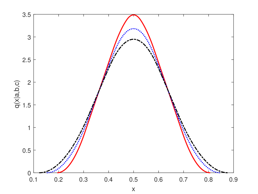
(a) $q(x|a,b,c)$ vs $x$

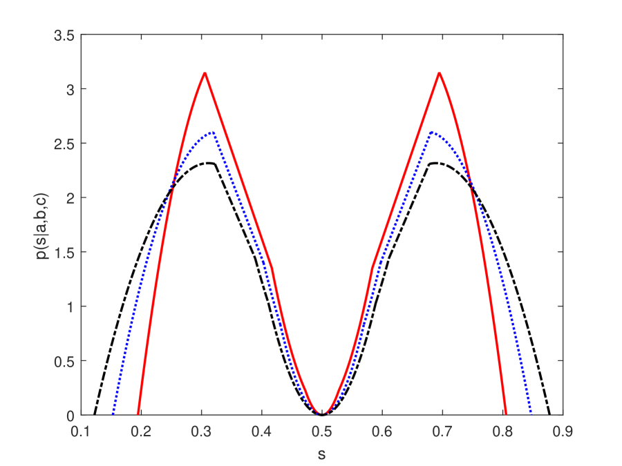
(b) $p(s|a,b,c)$ vs $s$

Figure 2: (a) The density function of the diagonal part $\rho^{D}_{s}$: $q(x|a,b,c)$ versus $x$. (b) The density function of an eigenvalue of $\rho_{s}$: $p(s|a,b,c)$ versus $s$. In either two figures, they are demonstrated with red line corresponding to $(a,b,c)=\left(\frac{1}{3},\frac{1}{6},\frac{1}{12}\right)$, blue line corresponding to $(a,b,c)=\left(\frac{1}{4},\frac{1}{8},\frac{1}{12}\right)$, black line corresponding to $(a,b,c)=\left(\frac{1}{5},\frac{1}{10},\frac{1}{15}\right)$.

From Figure 2, we see that the graphs of their distribution densities are symmetric with respect to the vertical line $\frac{1}{2}$ in the coordinate system. We find that for the mixture of three random density matrices, the density of a generic eigenvalue taking $\frac{1}{2}$ is vanished (see Fig 2(a)), but the density of a generic diagonal entry taking $\frac{1}{2}$ is largest (see Fig 2(b)). Note that $\left(\frac{1}{5},\frac{1}{10},\frac{1}{15}\right)\prec\left(\frac{1}{4},\frac{1}{8},\frac{1}{12}\right)\prec\left(\frac{1}{3},\frac{1}{6},\frac{1}{12}\right)$ . The common feature in the Figure 2(a&b) is the graphs rising up largely in the sense of the majorization order, i.e., the top of the graph corresponding to $\boldsymbol{p}$ is lower than that of the graph corresponding to $\boldsymbol{q}$ if $\boldsymbol{p}\prec\boldsymbol{q}$.

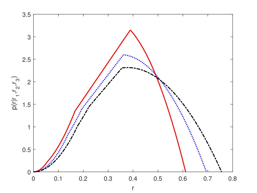
Figure 3: Reformulation of $p(s|a,b,c)$ in terms of Bloch lengths via $a=\frac{1-r_{1}}{2},b=\frac{1-r_{2}}{2},c=\frac{1-r_{3}}{2}$ and $s=\frac{1\pm r}{2}$: $p(r|r_{1},r_{2},r_{3})$ versus $r$ with red line corresponding to $(r_{1},r_{2},r_{3})=\left(\frac{1}{3},\frac{2}{3},\frac{5}{6}\right)$, blue line corresponding to $(r_{1},r_{2},r_{3})=\left(\frac{1}{2},\frac{3}{4},\frac{5}{6}\right)$, black line corresponding to $(r_{1},r_{2},r_{3})=\left(\frac{3}{5},\frac{4}{5},\frac{13}{15}\right)$.

3.3 The mixture of two qutrit states

Given $K=\mathrm{S}\mathrm{U}(3)$. Then $T=\left\{\mathrm{diag}(e^{\mathrm{i}\theta_{1}},e^{\mathrm{i}\theta_{2}},e^{\mathrm{i}\theta_{3}}):\theta_{1},\theta_{2},\theta_{3}\in\mathbb{R}\bigwedge\sum^{3}_{j=1}\theta_{j}=0\right\}$ with its Lie algebra $\mathfrak{t}=\left\{\mathrm{diag}(\mathrm{i}\theta_{1},\mathrm{i}\theta_{2},\mathrm{i}\theta_{3}):\theta_{1},\theta_{2},\theta_{3}\in\mathbb{R}\bigwedge\sum^{3}_{j=1}\theta_{j}=0\right\}$. Thus $\boldsymbol{h}_{1}=\mathrm{diag}(1,-1,0),\boldsymbol{h}_{2}=\mathrm{diag}(0,1,-1)$ is the basis of $\mathfrak{t}$, and $\mathfrak{t}=\mathrm{i}\mathbb{R}\cdot\boldsymbol{h}_{1}\oplus\mathrm{i}\mathbb{R}\cdot\boldsymbol{h}_{2}\cong\mathbb{R}^{2}$. All positive roots $\alpha_{ij}\in\mathfrak{t}^{*}$ with $i<j$, where $i,j\in\{1,2,3\}$, are given by $\alpha_{12}\cong\boldsymbol{h}_{1},\alpha_{13}\cong\boldsymbol{h}_{1}+\boldsymbol{h}_{2},\alpha_{23}\cong\boldsymbol{h}_{2}$. Note that the above realizations are via the Hilbert-Schmidt inner product. Furthermore, we can construct an orthonormal basis for $\mathrm{i}\mathfrak{t}$ as $\boldsymbol{h}_{x}=\frac{\boldsymbol{h}_{1}+\boldsymbol{h}_{2}}{\sqrt{2}},\boldsymbol{h}_{y}=\frac{\boldsymbol{h}_{1}-\boldsymbol{h}_{2}}{\sqrt{6}}$. Throughout this section, denote $u:=\sqrt{\frac{1}{2}}$ and $v:=\sqrt{\frac{3}{2}}$. Then all positive roots $\alpha_{ij}\in\mathfrak{t}^{*}$ with $i<j$, where $i,j\in\{1,2,3\}$, via $(\boldsymbol{h}_{x},\boldsymbol{h}_{y})$, are given by $\alpha_{12}\cong u\boldsymbol{h}_{x}+v\boldsymbol{h}_{y},\alpha_{13}\cong 2u\boldsymbol{h}_{x},\alpha_{23}\cong u\boldsymbol{h}_{x}-v\boldsymbol{h}_{y}$. Besides, the Weyl group is given by $W=S_{3}$. Let $\lambda\in\mathrm{i}\mathfrak{t}^{*}_{>0}$ and $\mu\in\mathrm{i}\mathfrak{t}^{*}_{\geqslant 0}$. We see that (2.5) reduces to the following: $\mathrm{DH}^{K}_{\mathcal{O}_{\lambda}\times\mathcal{O}_{\mu}}=\left(\sum_{w\in S_{3}}(-1)^{l(w)}\delta_{w\lambda}\right)*\mathrm{DH}^{T}_{\mathcal{O}_{\mu}}$, where $\mathrm{DH}^{T}_{\mathcal{O}_{\mu}}=\sum_{w\in S_{3}}(-1)^{l(w)}\delta_{w\mu}*H_{-\alpha_{12}}*H_{-\alpha_{13}}*H_{-\alpha_{23}}$. So,

$$\mathrm{DH}^{K}_{\mathcal{O}_{\lambda}\times\mathcal{O}_{\mu}}=\left(\sum_{w\in S_{3}}(-1)^{l(w)}\delta_{w\lambda}\right)*\left(\sum_{w\in S_{3}}(-1)^{l(w)}\delta_{w\mu}\right)*H_{-\alpha_{12}}*H_{-\alpha_{13}}*H_{-\alpha_{23}}\big{|}_{\mathrm{i}\mathfrak{t}^{*}_{\geqslant 0}}.$$ (3.19)

We see that $\lambda=(\lambda_{1},\lambda_{2},\lambda_{3})\in\mathrm{i}\mathfrak{t}^{*}_{>0}$, i.e., $\lambda_{1}>\lambda_{2}>\lambda_{3}$ and $\sum^{3}_{j=1}\lambda_{j}=0$. Note that $\lambda_{1}>0>\lambda_{3}$. With the orthonormal basis $\{\boldsymbol{h}_{x},\boldsymbol{h}_{y}\}$ of $\mathrm{i}\mathfrak{t}$, $\lambda\cong u(\lambda_{1}-\lambda_{3})\boldsymbol{h}_{x}+v(\lambda_{1}+\lambda_{3})\boldsymbol{h}_{y}\cong(u(\lambda_{1}-\lambda_{3}),v(\lambda_{1}+\lambda_{3}))$. Thus

$$\left(\sum_{w\in S_{3}}(-1)^{l(w)}\delta_{w\lambda}\right)*\left(\sum_{w\in S_{3}}(-1)^{l(w)}\delta_{w\mu}\right)=\sum_{w,w^{\prime}\in S_{3}}(-1)^{l(w)+l(w^{\prime})}\delta_{w\lambda+w^{\prime}\mu}.$$

Specifically, we see that, via $\{\boldsymbol{h}_{x},\boldsymbol{h}_{y}\}$,

$$(\lambda_{1},\lambda_{2},\lambda_{3})=\left(u(\lambda_{1}-\lambda_{3}),v(\lambda_{1}+\lambda_{3})\right),(\lambda_{1},\lambda_{3},\lambda_{2})=\left(u(2\lambda_{1}+\lambda_{3}),-v\lambda_{3}\right),$$

$$(\lambda_{2},\lambda_{1},\lambda_{3})=\left(-u(\lambda_{1}+2\lambda_{3}),-v\lambda_{1}\right),(\lambda_{2},\lambda_{3},\lambda_{1})=\left(-u(2\lambda_{1}+\lambda_{3}),-v\lambda_{3}\right),$$

$$(\lambda_{3},\lambda_{1},\lambda_{2})=\left(u(\lambda_{1}+2\lambda_{3}),-v\lambda_{1}\right),(\lambda_{3},\lambda_{2},\lambda_{1})=\left(-u(\lambda_{1}-\lambda_{3}),v(\lambda_{1}+\lambda_{3})\right).$$

Then

$$\sum_{w\in S_{3}}(-1)^{l(w)}\delta_{w\lambda} = \delta_{\left(u(\lambda_{1}-\lambda_{3}),v(\lambda_{1}+\lambda_{3})\right)}+\delta_{\left(u(\lambda_{1}+2\lambda_{3}),-v\lambda_{1}\right)}+\delta_{\left(-u(2\lambda_{1}+\lambda_{3}),-v\lambda_{3}\right)}$$

$$-\delta_{\left(u(2\lambda_{1}+\lambda_{3}),-v\lambda_{3}\right)}-\delta_{\left(-u(\lambda_{1}+2\lambda_{3}),-v\lambda_{1}\right)}-\delta_{\left(-u(\lambda_{1}-\lambda_{3}),v(\lambda_{1}+\lambda_{3})\right)}.$$

Proposition 3.10.

The measure $H_{-\alpha_{12}}*H_{-\alpha_{13}}*H_{-\alpha_{23}}=H_{-\boldsymbol{h}_{1}}*H_{-\boldsymbol{h}_{1}-\boldsymbol{h}_{2}}*H_{-\boldsymbol{h}_{2}}$ has Lebesgue density:

$$f(\nu)=\frac{1}{\sqrt{3}}\times\begin{cases}0,&\text{if }\nu\in C_{0};\\ -\nu_{1},&\text{if }\nu\in C_{1};\\ \nu_{3},&\text{if }\nu\in C_{2}.\end{cases}$$ (3.20)

Here $C_{0}$ is the complementary region of the positive cone formed by three vectors $\{-\boldsymbol{h}_{1},-\boldsymbol{h}_{1}-\boldsymbol{h}_{2},-\boldsymbol{h}_{2}\}$, $C_{1}$ is the positive cone generated by $\{-\boldsymbol{h}_{1},-\boldsymbol{h}_{1}-\boldsymbol{h}_{2}\}$, and $C_{2}$ is the positive cone generated by $\{-\boldsymbol{h}_{1}-\boldsymbol{h}_{2},-\boldsymbol{h}_{2}\}$.

The first proof.

In the present proof, we follow up the method used in [8], where Paradan’s wall-crossing formula [5] are heavily used. The measure $H_{-\boldsymbol{h}_{1}}*H_{-\boldsymbol{h}_{1}-\boldsymbol{h}_{2}}*H_{-\boldsymbol{h}_{2}}$ is, in fact, the non-Abelian Duistermaat-Heckman measure that is on the closures of the regular chambers containing the vertex $(0,0)$ given by the convolution $\delta_{(0,0,0)}*H_{-\boldsymbol{h}_{1}}*H_{-\boldsymbol{h}_{1}-\boldsymbol{h}_{2}}*H_{-\boldsymbol{h}_{2}}\cong\delta_{(0,0)}*H_{\left(-u,-v\right)}*H_{(-2u,0)}*H_{\left(-u,v\right)}$. Its density is denoted by $f(\nu)\cong f(u(\nu_{1}-\nu_{3}),v(\nu_{1}+\nu_{3}))$. Thus $\omega_{1}=\left(-u,v\right),\omega_{2}=\left(-2u,0\right),\omega_{3}=\left(-u,-v\right)$.
(i) Clearly $f\equiv 0$ on $C_{0}$. The wall $W_{01}$ separating $C_{0}$ and $C_{1}$ is given by the equation: $\frac{x}{-1}=\frac{y}{\sqrt{3}}$. Its normal vector $\xi_{01}=(-\sqrt{3},-1)$. Just only one weights $\omega_{1}=\left(-u,v\right)$ lies on the linear hyperplane spanned by $W_{01}$ (other weights are outside of $W_{01}$: $\omega_{2}=\left(-2u,0\right),\omega_{3}=\left(-u,-v\right)$). Consider the push-forward of Lebesgue measure on $\mathbb{R}_{\geqslant 0}$ along the linear map $P_{W_{01}}:t\mapsto t\omega_{1}$. Its density with respect to $\mathrm{d}w$ is given by a single homogeneous polynomial on the wall $W_{01}$. Denote by $f_{W_{01}}$ any polynomial function extending it to all of $\mathrm{i}\mathfrak{t}^{*}$, the Lie algebra $\mathrm{S}\mathrm{U}(3)$. Clearly $f_{W_{01}}=\sqrt{2}$. Indeed,

$$f^{-1}_{W_{01}}=\mathrm{d}\lambda(\omega_{1},\xi_{01}/\left\lVert\mspace{1.0mu}\xi_{01}\mspace{1.0mu}\right\rVert^{2})=\left\lVert\mspace{1.0mu}\begin{array}[]{cc}-u&v\\ -\frac{\sqrt{3}}{4}&-\frac{1}{4}\end{array}\mspace{1.0mu}\right\rVert=\frac{1}{\sqrt{2}}.$$

Hence

$$f(\nu)=\sqrt{2}\mathrm{Res}_{z=0}\left(\frac{e^{\left\langle\nu,\boldsymbol{x}+z\xi_{01}\right\rangle}}{\left\langle\omega_{2},\boldsymbol{x}+z\xi_{01}\right\rangle\left\langle\omega_{3},\boldsymbol{x}+z\xi_{01}\right\rangle}\right)_{\boldsymbol{x}=0},$$

Thus

$$f(\nu)=\sqrt{2}\times\mathrm{Res}_{z=0}\left(\frac{\exp\left(-\sqrt{6}\nu_{1}z\right)}{6z^{2}}\right).$$

Therefore, on the chamber $C_{1}$, $f(\nu)=-\frac{1}{\sqrt{3}}\nu_{1}$.
(ii) The wall $W_{12}$ separating $C_{1}$ and $C_{2}$ is given by the equation: $y=0$. Its normal vector $\xi_{12}=(0,-1)$. Just only one weights $\omega_{2}=(-2u,0)$ lies on the linear hyperplane spanned by $W_{12}$ (other weights are outside of $W_{12}$: $\omega_{1}=\left(-u,v\right),\omega_{3}=\left(-u,-v\right)$). Consider the push-forward of Lebesgue measure on $\mathbb{R}_{\geqslant 0}$ along the linear map $P_{W_{12}}:t\mapsto t\omega_{2}$. Its density with respect to $\mathrm{d}w$ is given by a single homogeneous polynomial on the wall $W_{12}$. Denote by $f_{W_{12}}$ any polynomial function extending it to all of $\mathrm{i}\mathfrak{t}^{*}$, the Lie algebra $\mathrm{S}\mathrm{U}(3)$. Clearly $f_{W_{12}}=\frac{1}{\sqrt{2}}$. Indeed,

$$f^{-1}_{W_{12}}=\mathrm{d}\lambda(\omega_{2},\xi_{12}/\left\lVert\mspace{1.0mu}\xi_{12}\mspace{1.0mu}\right\rVert^{2})=\left\lVert\mspace{1.0mu}\begin{array}[]{cc}-2u&0\\ 0&-1\end{array}\mspace{1.0mu}\right\rVert=\sqrt{2}.$$

Hence

$$f(\nu)-\left(-\frac{1}{\sqrt{3}}\nu_{1}\right)=\frac{1}{\sqrt{2}}\mathrm{Res}_{z=0}\left(\frac{e^{\left\langle\nu,\boldsymbol{x}+z\xi_{12}\right\rangle}}{\left\langle\omega_{1},\boldsymbol{x}+z\xi_{12}\right\rangle\left\langle\omega_{3},\boldsymbol{x}+z\xi_{12}\right\rangle}\right)_{\boldsymbol{x}=0}.$$

Thus

$$f(\nu)+\frac{1}{\sqrt{3}}\nu_{1}=\frac{1}{\sqrt{2}}\times\mathrm{Res}_{z=0}\left(\frac{\exp\left(-\sqrt{\frac{3}{2}}(\nu_{1}+\nu_{3})z\right)}{-\frac{3}{2}z^{2}}\right)$$

Therefore, on the chamber $C_{2}$, $f(\nu)=\frac{1}{\sqrt{3}}\nu_{3}$. In summary, we obtain the desired identity (3.20). This completes the proof. ∎

If we denote by $(x,y)=\left(u(\nu_{1}-\nu_{3}),v(\nu_{1}+\nu_{3})\right)$, then the above result can be reformulated as

$$f(x,y)=\begin{cases}\frac{\left\lvert\mspace{1.0mu}y\mspace{1.0mu}\right\rvert-\sqrt{3}x}{3\sqrt{2}},&\text{if }(x,y)\in\left\{(x,y)\in\mathbb{R}^{2}:x\leqslant 0,\sqrt{3}x\leqslant y\leqslant-\sqrt{3}x\right\},\\ 0,&\text{otherwise}.\end{cases}$$ (3.23)

The support of this binary function in (3.23) and its graph are depicted in Figure 4.

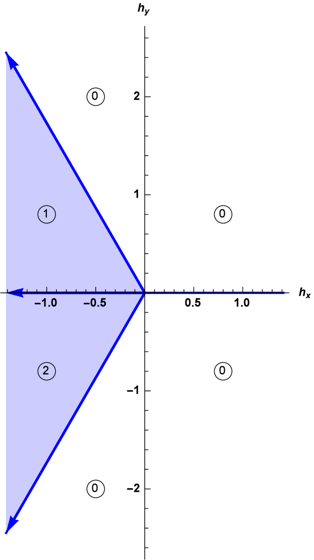
(a) Chambers and support (Shadow region)

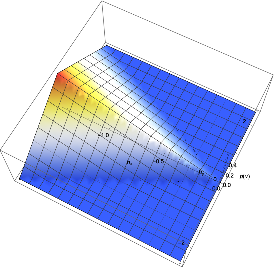
(b) The density function (3.23) of the iterated convolution computed in Proposition 3.10

Figure 4: The support of the iterated convolution in Proposition 3.10 and its density over the support

The second proof.

The measure $H_{-\boldsymbol{h}_{1}}*H_{-\boldsymbol{h}_{1}-\boldsymbol{h}_{2}}*H_{-\boldsymbol{h}_{2}}$ is equivalently given by the convolution

$$H_{\left(-u,-v\right)}*H_{(-2u,0)}*H_{\left(-u,v\right)}.$$

Denote by $\mathscr{C}$ the positive cone generated by three vectors $(-u,-v),(-2u,0),(-u,v)$, i.e., $\mathscr{C}_{3}:=C_{1}\cup C_{2}$ in Figure 4, and $C_{0}=\mathbb{R}^{2}\backslash\mathscr{C}_{3}$. We can directly compute its density:

$$\int^{\infty}_{0}\mathrm{d}t_{1}\int^{\infty}_{0}\mathrm{d}t_{2}\int^{\infty}_{0}\mathrm{d}t_{3}\delta\left(t_{1}\left(\begin{array}[]{c}-u\\ -v\end{array}\right)+t_{2}\left(\begin{array}[]{c}-u\\ v\end{array}\right)+t_{3}\left(\begin{array}[]{c}-2u\\ 0\end{array}\right)-\left(\begin{array}[]{c}x\\ y\end{array}\right)\right)$$

$$=\int^{\infty}_{0}\mathrm{d}t_{1}\int^{\infty}_{0}\mathrm{d}t_{2}\int^{\infty}_{0}\mathrm{d}t_{3}\delta\left(\left(\begin{array}[]{c}u(-t_{1}-t_{2})\\ u\sqrt{3}(-t_{1}+t_{2})\end{array}\right)+\left(\begin{array}[]{c}-2ut_{3}-x\\ -y\end{array}\right)\right).$$

By change of variables, i.e., $s_{1}=u(t_{1}+t_{2}),s_{2}=\sqrt{3}u(t_{1}-t_{2})$, we get that the density is given by

$$\frac{1}{\sqrt{3}}\int^{\infty}_{0}\mathrm{d}s_{1}\int^{\infty}_{-\infty}\mathrm{d}s_{2}\int^{\infty}_{0}\mathrm{d}t_{3}\delta\left(\left(\begin{array}[]{c}-s_{1}\\ -s_{2}\end{array}\right)-\left(\begin{array}[]{c}2ut_{3}+x\\ y\end{array}\right)\right)$$

$$=\frac{1}{\sqrt{3}}\int^{\infty}_{0}\mathrm{d}t_{3}\mathbf{\mathbb{1}}_{\mathscr{C}}\left(-\left(\begin{array}[]{c}2ut_{3}+x\\ y\end{array}\right)\right)$$

Now $-\left(\begin{array}[]{c}2ut_{3}+x\\ y\end{array}\right)\in\mathscr{C}$ if and only if $\left\lvert\mspace{1.0mu}y\mspace{1.0mu}\right\rvert\leqslant\sqrt{3}\left\lvert\mspace{1.0mu}2ut_{3}+x\mspace{1.0mu}\right\rvert\leqslant\sqrt{3}x$ and $x\leqslant 2ut_{3}+x\leqslant-\frac{\left\lvert\mspace{1.0mu}y\mspace{1.0mu}\right\rvert}{\sqrt{3}}$, i.e., $0\leqslant t_{3}\leqslant\frac{\left\lvert\mspace{1.0mu}y\mspace{1.0mu}\right\rvert}{\sqrt{6}}-\frac{x}{\sqrt{2}}$. Therefore the density is given by $\frac{1}{\sqrt{3}}\int^{\frac{\left\lvert\mspace{1.0mu}y\mspace{1.0mu}\right\rvert}{\sqrt{6}}-\frac{x}{\sqrt{2}}}_{0}\mathrm{d}t_{3}=\frac{\left\lvert\mspace{1.0mu}y\mspace{1.0mu}\right\rvert-\sqrt{3}x}{3\sqrt{2}}$. The support for this density function is $\mathscr{C}_{3}=\left\{(x,y)\in\mathbb{R}^{2}:x\leqslant 0,\sqrt{3}x\leqslant y\leqslant-\sqrt{3}x\right\}$. ∎

Example 3.11.

Let $u=\sqrt{\frac{1}{2}}$ and $v=\sqrt{\frac{3}{2}}$. Let $\lambda_{1}=\frac{1}{6},\lambda_{2}=0,\lambda_{3}=-\frac{1}{6}$ and $\mu_{1}=\frac{1}{3},\mu_{2}=-\frac{1}{12},\mu_{3}=-\frac{1}{4}$. The density of the non-Abelian D-H measure is given by the restriction to the positive Weyl chamber of an alternating sum of 36 copies of the density described in Proposition 3.10. Note that the geometry of the support of the density described in Proposition 3.10, it is easily seen that only summands for points in the shaded region, i.e., $\left\{(x,y)\in\mathbb{R}^{2}:x\geqslant 0,-\sqrt{3}x\leqslant y\leqslant\sqrt{3}x\right\}$ contribute, see Figure 5 (a). Clearly the shaded region is a convex cone generated by three positive roots $\left\{\alpha_{12},\alpha_{13},\alpha_{23}\right\}$. From Eq. (3.19), we can pick out the following ten points which are falling in such convex cone:

$$\left(\frac{11u}{12},\frac{v}{12}\right),\left(\frac{7u}{12},\frac{5v}{12}\right),\left(\frac{7u}{12},\frac{v}{12}\right),\left(\frac{5u}{12},\frac{v}{4}\right),\left(\frac{5u}{12},-\frac{v}{12}\right),$$

$$\left(\frac{u}{3},-\frac{v}{6}\right),\left(\frac{3u}{4},\frac{v}{4}\right),\left(\frac{3u}{4},-\frac{v}{12}\right),\left(\frac{u}{2},-\frac{v}{3}\right),\left(\frac{u}{4},\frac{v}{12}\right).$$

Therefore,

$$\mathrm{DH}^{K}_{\mathcal{O}_{\lambda}\times\mathcal{O}_{\mu}} = \left(\delta_{\left(\frac{11u}{12},\frac{v}{12}\right)}+\delta_{\left(\frac{7u}{12},\frac{5v}{12}\right)}+\delta_{\left(\frac{7u}{12},\frac{v}{12}\right)}+\delta_{\left(\frac{5u}{12},\frac{v}{4}\right)}+\delta_{\left(\frac{5u}{12},-\frac{v}{12}\right)}+\delta_{\left(\frac{u}{3},-\frac{v}{6}\right)}\right.$$

$$\left.~{}~{}~{}-2\delta_{\left(\frac{3u}{4},\frac{v}{4}\right)}-\delta_{\left(\frac{3u}{4},-\frac{v}{12}\right)}-\delta_{\left(\frac{u}{2},-\frac{v}{3}\right)}-2\delta_{\left(\frac{u}{4},\frac{v}{12}\right)}\right)*H_{-\alpha_{12}}*H_{-\alpha_{13}}*H_{-\alpha_{23}}\big{|}_{\mathrm{i}\mathfrak{t}^{*}_{\geqslant 0}}.$$

Here the positive Weyl chamber $\mathrm{i}\mathfrak{t}^{*}_{\geqslant 0}$ is identified with $\left\{(x,y)\in\mathbb{R}^{2}:x\geqslant 0,-\frac{1}{\sqrt{3}}x\leqslant y\leqslant\frac{1}{\sqrt{3}}x\right\}$, see Figure 5(a).

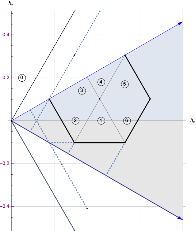
(a) Chambers and support $\mathscr{S}_{3}=\bigcup^{6}_{j=1}C_{j}$

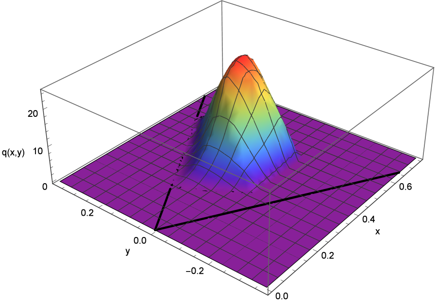
(b) The density function (3.28) of $(\tau_{K})_{*}(\Phi_{K})_{*}\left(\frac{\mu_{M}}{\mathrm{vol}(M)}\right)$

Figure 5: The support of the iterated convolution and its density over the support for Example 3.11

The density of the non-Abelian D-H measure is given as

$$p(x,y)=\begin{cases}0,&\text{if }(x,y)\in C_{0};\\ \frac{24y+\sqrt{6}}{36\sqrt{2}},&\text{if }(x,y)\in C_{1};\\ \frac{6\sqrt{3}x+6y-\sqrt{6}}{18\sqrt{2}},&\text{if }(x,y)\in C_{2};\\ \frac{x-\sqrt{3}y}{\sqrt{6}},&\text{if }(x,y)\in C_{3}\cup C_{4};\\ \frac{\sqrt{6}-2\sqrt{3}x-2y}{6\sqrt{2}},&\text{if }(x,y)\in C_{5};\\ \frac{5\sqrt{6}-12\sqrt{3}x+12y}{36\sqrt{2}},&\text{if }(x,y)\in C_{6}.\end{cases}$$

Here all $C_{j}$’s are the corresponding regions, marked by the circled-numbers in Figure 5(a). We have already known that

$$(\tau_{K})_{*}(\Phi_{K})_{*}\left(\frac{\mu_{M}}{\mathrm{vol}(M)}\right)=p_{K}\frac{\mathrm{DH}^{K}_{M}}{\mathrm{vol}(M)},$$

where $p_{K}(\nu)=\frac{(\nu_{1}-\nu_{2})(\nu_{1}-\nu_{3})(\nu_{2}-\nu_{3})}{2}$. Then $p_{K}(\nu)$, via $(x,y)=\left(u(\nu_{1}-\nu_{3}),v(\nu_{1}+\nu_{3})\right)$, can be rewritten as

$$p_{K}(x,y)=\frac{x^{3}-3xy^{2}}{2\sqrt{2}},\quad(x,y)\in\left\{(x,y)\in\mathbb{R}^{2}:x\geqslant 0,-\frac{1}{\sqrt{3}}x\leqslant y\leqslant\frac{1}{\sqrt{3}}x\right\}.$$

and $\mathrm{vol}(M)=\mathrm{vol}(\mathcal{O}_{\lambda})\mathrm{vol}(\mathcal{O}_{\mu})=p_{K}\left(\frac{u}{3},0\right)p_{K}\left(\frac{7u}{12},\frac{v}{12}\right)=\frac{35}{373248}$. Therefore the density (see Figure 5(b)) for $(\tau_{K})_{*}(\Phi_{K})_{*}\left(\frac{\mu_{M}}{\mathrm{vol}(M)}\right)$ (with the support being $\mathscr{S}_{3}:=\bigcup^{6}_{j=1}C_{j}$) is given as

$$q(x,y)=\frac{2^{5}3^{4}(x^{3}-3xy^{2})}{35}\times\begin{cases}0,&\text{if }(x,y)\in C_{0};\\ 24y+\sqrt{6},&\text{if }(x,y)\in C_{1};\\ 12\sqrt{3}x+12y-2\sqrt{6},&\text{if }(x,y)\in C_{2};\\ 12\sqrt{3}x-36y,&\text{if }(x,y)\in C_{3}\cup C_{4};\\ 6\sqrt{6}-12\sqrt{3}x-12y,&\text{if }(x,y)\in C_{5};\\ 5\sqrt{6}-12\sqrt{3}x+12y,&\text{if }(x,y)\in C_{6}.\end{cases}$$ (3.28)

The normalization of the above function (3.28), i.e., the integration over the support being equal to one, is easily checked by computer system. Consider the following random quantum state $\rho=\frac{U\boldsymbol{\lambda}_{1}U^{\dagger}+V\boldsymbol{\lambda}_{2}V^{\dagger}}{2}$, where $U,V$ are sampled by Haar measure over the unitary group and $\boldsymbol{\lambda}_{1}=\mathrm{diag}(\frac{1}{2},\frac{1}{3},\frac{1}{6})$ and $\boldsymbol{\lambda}_{2}=\mathrm{diag}(\frac{2}{3},\frac{1}{4},\frac{1}{12})$. Then $2\left(\rho-\frac{\mathbb{1}_{3}}{3}\right)=U\mathrm{diag}\left(\frac{1}{6},0,-\frac{1}{6}\right)U^{\dagger}+V\mathrm{diag}\left(\frac{1}{3},-\frac{1}{12},-\frac{1}{4}\right)V^{\dagger}$. Let $s=\lambda_{\max}(\rho),t=\lambda_{\min}(\rho)$ be respective maximal and minimal eigenvalues of $\rho$. Denote the eigenvalue vector of random qubtrit $\rho$ by $(s,1-s-t,t)$, ordered decreasingly. Thus the eigenvalue vector of $2(\rho-\mathbb{1}/3)$ is $\left(2(s-1/3),2(2/3-s-t),2(t-1/3)\right)$. Its 2D coordinate via $(\boldsymbol{h}_{x},\boldsymbol{h}_{y})$ is identified with $(x,y)$. Then

$$x=2u(s-t),y=2v\left(s+t-\frac{2}{3}\right)\quad\text{or}\quad s=\frac{1}{4}\left(\frac{y}{v}+\frac{x}{u}\right)+\frac{1}{3},t=\frac{1}{4}\left(\frac{y}{v}-\frac{x}{u}\right)+\frac{1}{3}.$$

Therefore we can draw the conclusion that the joint density of $(s,t)$ is given by

$$f(s,t)=\frac{2^{14}\cdot 3^{6}}{5\cdot 7}(s-t)\left(2s^{2}+2t^{2}+5st-3s-3t+1\right)\cdot\Delta(s,t),$$ (3.29)

where

$$\Delta(s,t):=\begin{cases}s+2t-1,&\text{if }(s,t)\in\left\{(s,t):\frac{5}{12}\leqslant s\leqslant\frac{7}{12},\max\left(\frac{17-24s}{24},\frac{5}{24}\right)\leqslant t\leqslant\frac{1-s}{2}\right\};\\ \frac{5}{8}-s-t,&\text{if }(s,t)\in\left\{(s,t):\frac{5}{12}\leqslant s\leqslant\frac{1}{2},\frac{5-8s}{8}\leqslant t\leqslant\frac{5}{24}\right\};\\ \frac{5}{12}-s,&\text{if }(s,t)\in\left\{(s,t):\frac{5}{12}\leqslant s\leqslant\frac{1}{2},\frac{5}{24}\leqslant t\leqslant\frac{17-24s}{24}\right\};\\ s-\frac{7}{12},&\text{if }(s,t)\in\left\{(s,t):\frac{1}{2}\leqslant s\leqslant\frac{7}{12},\frac{17-24s}{24}\leqslant t\leqslant\frac{5}{24}\right\};\\ \frac{1}{8}-t,&\text{if }(s,t)\in\left\{(s,t):\frac{1}{2}\leqslant s\leqslant\frac{7}{12},\frac{1}{8}\leqslant t\leqslant\frac{17-24s}{24}\right\}.\end{cases}$$

The support of the density function (3.29) are plotted in the following Figure 6:

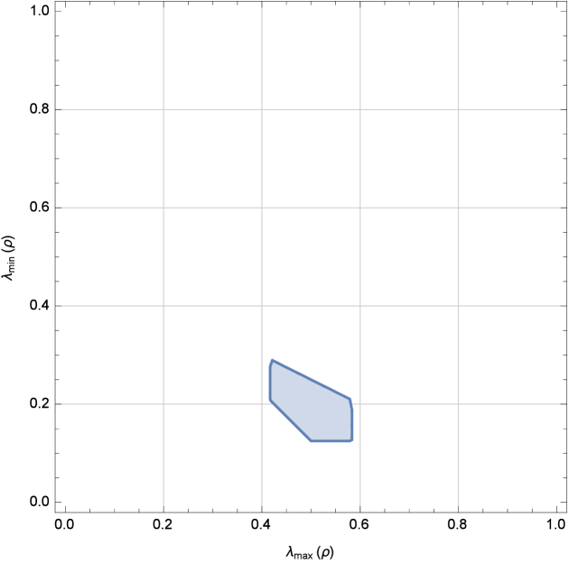
(a) Support

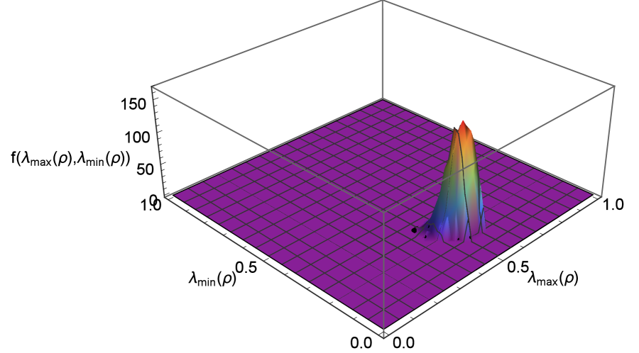
(b) Density function over the support

Figure 6: (a) The feasible region of the maximal and minimal eigenvalues of a random qutrit $\rho=\frac{1}{2}\left(U\boldsymbol{\lambda}_{1}U^{\dagger}+V\boldsymbol{\lambda}_{2}V^{\dagger}\right)$ where $\boldsymbol{\lambda}_{1}=\left(\frac{1}{2},\frac{1}{3},\frac{1}{6}\right),\boldsymbol{\lambda}_{2}=\left(\frac{2}{3},\frac{1}{4},\frac{1}{12}\right)$ and $U,V\in\mathrm{S}\mathrm{U}(3)$ are Haar-distributed; (b) The joint density function of the maximal and minimal eigenvalues of a random qutrit $\rho=\frac{1}{2}\left(U\boldsymbol{\lambda}_{1}U^{\dagger}+V\boldsymbol{\lambda}_{2}V^{\dagger}\right)$

Remark 3.12.

From the Example 3.11, we see that the reasoning method used in the Example 3.11 essentially provide a complete solution to the joint density function of eigenvalues of the mixture of quantum states algorithmically. That is, once two spectra are given, we can give a analytical solution based on the given spectra. Unfortunately, there is no unifying formula for that problem.

3.4 The mixture of two two-qubit states

Given $K=\mathrm{S}\mathrm{U}(4)$. Then $T=\left\{\mathrm{diag}(e^{\mathrm{i}\theta_{1}},e^{\mathrm{i}\theta_{2}},e^{\mathrm{i}\theta_{3}},e^{\mathrm{i}\theta_{4}}):\theta_{1},\theta_{2},\theta_{3},\theta_{4}\in\mathbb{R}\bigwedge\sum^{4}_{j=1}\theta_{j}=0\right\}$ with its Lie algebra $\mathfrak{t}=\left\{\mathrm{diag}(\mathrm{i}\theta_{1},\mathrm{i}\theta_{2},\mathrm{i}\theta_{3},\mathrm{i}\theta_{4}):\theta_{1},\theta_{2},\theta_{3},\theta_{4}\in\mathbb{R}\bigwedge\sum^{4}_{j=1}\theta_{j}=0\right\}$. Thus $\boldsymbol{h}_{1}=\mathrm{diag}(1,-1,0,0)$, $\boldsymbol{h}_{2}=\mathrm{diag}(0,1,-1,0)$, $\boldsymbol{h}_{3}=\mathrm{diag}(0,0,1,-1)$ is the basis of $\mathfrak{t}$, and $\mathfrak{t}=\mathrm{i}\mathbb{R}\cdot\boldsymbol{h}_{1}\oplus\mathrm{i}\mathbb{R}\cdot\boldsymbol{h}_{2}\oplus\mathrm{i}\mathbb{R}\cdot\boldsymbol{h}_{3}\cong\mathbb{R}^{3}$. All positive roots $\alpha_{ij}\in\mathfrak{t}^{*}$ with $i<j$, where $i,j\in\{1,2,3,4\}$, are given by $\alpha_{12}\cong\boldsymbol{h}_{1},\alpha_{13}\cong\boldsymbol{h}_{1}+\boldsymbol{h}_{2},\alpha_{14}\cong\boldsymbol{h}_{1}+\boldsymbol{h}_{2}+\boldsymbol{h}_{3},\alpha_{23}\cong\boldsymbol{h}_{2},\alpha_{24}\cong\boldsymbol{h}_{2}+\boldsymbol{h}_{3},\alpha_{34}\cong\boldsymbol{h}_{3}$. Note that the above realizations are via the Hilbert-Schmidt inner product. Furthermore, we can construct an orthonormal basis for $\mathrm{i}\mathfrak{t}$ as follows:

$$\boldsymbol{h}_{x}=\frac{\boldsymbol{h}_{1}}{\sqrt{2}},\quad\boldsymbol{h}_{y}=\frac{\boldsymbol{h}_{3}}{\sqrt{2}},\quad\boldsymbol{h}_{z}=\frac{\boldsymbol{h}_{1}+2\boldsymbol{h}_{2}+\boldsymbol{h}_{3}}{2}.$$ (3.30)

Denote also $u=\sqrt{\frac{1}{2}}$. Then all positive roots $\alpha_{ij}\in\mathfrak{t}^{*}$ with $i<j$, where $i,j\in\{1,2,3,4\}$, via $(\boldsymbol{h}_{x},\boldsymbol{h}_{y},\boldsymbol{h}_{z})$, are given by $\alpha_{12}=(2u,0,0),\alpha_{13}=\left(u,-u,1\right),\alpha_{14}=\left(u,u,1\right),\alpha_{23}=\left(-u,-u,1\right),\alpha_{24}=\left(-u,u,1\right),\alpha_{34}=(0,2u,0)$. Besides, the Weyl group is given by $W=S_{4}$. Let $\lambda\in\mathrm{i}\mathfrak{t}^{*}_{>0}$ and $\mu\in\mathrm{i}\mathfrak{t}^{*}_{\geqslant 0}$. So,

$$\mathrm{DH}^{K}_{\mathcal{O}_{\lambda}\times\mathcal{O}_{\mu}}=\left(\sum_{w,w^{\prime}\in S_{4}}(-1)^{l(w)+l(w^{\prime})}\delta_{w\lambda+w^{\prime}\mu}\right)*H_{-\alpha_{12}}*H_{-\alpha_{13}}*H_{-\alpha_{14}}*H_{-\alpha_{23}}*H_{-\alpha_{24}}*H_{-\alpha_{34}}\big{|}_{\mathrm{i}\mathfrak{t}^{*}_{\geqslant 0}}.$$

We see that $\lambda=(\lambda_{1},\lambda_{2},\lambda_{3},\lambda_{4})\in\mathrm{i}\mathfrak{t}^{*}_{>0}$, i.e., $\lambda_{1}>\lambda_{2}>\lambda_{3}>\lambda_{4}$ and $\sum^{4}_{j=1}\lambda_{j}=0$. From this, we get that $\lambda_{1}>0>\lambda_{4},\lambda_{1}+\lambda_{2}>0>\lambda_{3}+\lambda_{4}$. With the orthonormal basis $\{\boldsymbol{h}_{x},\boldsymbol{h}_{y},\boldsymbol{h}_{z}\}$ of $\mathrm{i}\mathfrak{t}$, $\lambda\cong\left(u(\lambda_{1}-\lambda_{2}),-u(\lambda_{1}+\lambda_{2}+2\lambda_{4}),\lambda_{1}+\lambda_{2}\right)$, where $u(\lambda_{1}-\lambda_{2})>0,\lambda_{1}+\lambda_{2}>0$. In the following, we calculate the density of the measure $H_{-\alpha_{12}}*H_{-\alpha_{13}}*H_{-\alpha_{14}}*H_{-\alpha_{23}}*H_{-\alpha_{24}}*H_{-\alpha_{34}}$.

Proposition 3.13.

The measure $H_{-\alpha_{12}}*H_{-\alpha_{13}}*H_{-\alpha_{14}}*H_{-\alpha_{23}}*H_{-\alpha_{24}}*H_{-\alpha_{34}}$ has Lebesgue density:

$$f(\nu)=-\frac{1}{8}(\nu_{1}+\nu_{2})(3\nu_{1}+\nu_{2})(\nu_{1}+\nu_{2}-2\nu_{4}).$$ (3.31)

Proof.

Now the measure $H_{-\alpha_{12}}*H_{-\alpha_{13}}*H_{-\alpha_{14}}*H_{-\alpha_{23}}*H_{-\alpha_{24}}*H_{-\alpha_{34}}$ is represented by (via $(\boldsymbol{h}_{x},\boldsymbol{h}_{y},\boldsymbol{h}_{z})$)

$$\delta_{(0,0,0)}*H_{(-2u,0,0)}*H_{(-u,u,-1)}*H_{(-u,-u,-1)}*H_{(u,u,-1)}*H_{(u,-u,-1)}*H_{(0,-2u,0)}.$$

Note that $t_{1}(-2u,0,0)+t_{2}(0,-2u,0)+t_{3}(u,u,-1)+t_{4}(-u,u,-1)+t_{5}(-u,-u,-1)+t_{6}(u,-u,-1)$ is equal to

$$(u(-2t_{1}+t_{3}),u(-2t_{2}+t_{3}),-t_{3})+(u(-t_{4}-t_{5}+t_{6}),u(t_{4}-t_{5}-t_{6}),-t_{4}-t_{5}-t_{6}).$$

Its density of the above measure can be computed in the following:

$$\iiint\iiint_{\mathbb{R}^{6}_{+}}\mathrm{d}t_{1}\mathrm{d}t_{2}\mathrm{d}t_{3}\mathrm{d}t_{4}\mathrm{d}t_{5}\mathrm{d}t_{6}\delta\left(\left(\begin{array}[]{c}u(-2t_{1}+t_{3})\\ u(-2t_{2}+t_{3})\\ -t_{3}\end{array}\right)+\left(\begin{array}[]{c}u(-t_{4}-t_{5}+t_{6})\\ u(t_{4}-t_{5}-t_{6})\\ -t_{4}-t_{5}-t_{6}\end{array}\right)-\left(\begin{array}[]{c}x\\ y\\ z\end{array}\right)\right),$$

where $\nu=x\boldsymbol{h}_{x}+y\boldsymbol{h}_{y}+z\boldsymbol{h}_{z}\cong(x,y,z)$. Then performing change of variables $s_{1}=u(2t_{1}-t_{3}),s_{2}=u(2t_{2}-t_{3}),s_{3}=t_{3}$, we get the density

$$\frac{1}{2}\iiint\iiint\mathrm{d}s_{1}\mathrm{d}s_{2}\mathrm{d}s_{3}\mathrm{d}t_{4}\mathrm{d}t_{5}\mathrm{d}t_{6}\delta\left(\left(\begin{array}[]{c}-s_{1}\\ -s_{2}\\ -s_{3}\end{array}\right)-\left(\begin{array}[]{c}u(t_{4}+t_{5}-t_{6})+x\\ u(-t_{4}+t_{5}+t_{6})+y\\ t_{4}+t_{5}+t_{6}+z\end{array}\right)\right)$$

$$=\frac{1}{2}\iiint\mathrm{d}t_{4}\mathrm{d}t_{5}\mathrm{d}t_{6}\mathbf{\mathbb{1}}_{\mathscr{D}}\left(\begin{array}[]{c}u(t_{4}+t_{5}-t_{6})+x\\ u(-t_{4}+t_{5}+t_{6})+y\\ t_{4}+t_{5}+t_{6}+z\end{array}\right),$$

where $\mathscr{D}$ is the positive cone generated by $(-2u,0,0),(0,-2u,0),(u,u,-1)$. Now

$$\left(u(t_{4}+t_{5}-t_{6})+x,u(-t_{4}+t_{5}+t_{6})+y,t_{4}+t_{5}+t_{6}+z\right)\in\mathscr{D}$$

if and only if

$$\begin{cases}0\leqslant t_{j},j=4,5,6;\\ 0\leqslant t_{4}+t_{5}+t_{6}\leqslant\left\lvert\mspace{1.0mu}z\mspace{1.0mu}\right\rvert;\\ 0\leqslant 3t_{4}+3t_{5}+t_{6}\leqslant\sqrt{2}(\sqrt{2}\left\lvert\mspace{1.0mu}z\mspace{1.0mu}\right\rvert-x);\\ 0\leqslant t_{4}+3t_{5}+3t_{6}\leqslant\sqrt{2}(\sqrt{2}\left\lvert\mspace{1.0mu}z\mspace{1.0mu}\right\rvert-y).\end{cases}$$ (3.35)

where

$$z\leqslant 0,x\leqslant\sqrt{2}\left\lvert\mspace{1.0mu}z\mspace{1.0mu}\right\rvert,y\leqslant\sqrt{2}\left\lvert\mspace{1.0mu}z\mspace{1.0mu}\right\rvert.$$ (3.36)

Let $R(x,y,z)$ be the region determined by (3.35) whenever $x,y,z$ satisfying (3.36). Then the density is given by

$$\frac{1}{2}\iiint_{R(x,y,z)}\mathrm{d}t_{4}\mathrm{d}t_{5}\mathrm{d}t_{6}=\frac{1}{2}\mathrm{vol}(R(x,y,z)).$$

Performing change of variables $\alpha=t_{4}+t_{5}+t_{6},\beta=3t_{4}+3t_{5}+t_{6},\gamma=t_{4}+3t_{5}+3t_{6}$, we obtain that $\mathrm{d}t_{4}\mathrm{d}t_{5}\mathrm{d}t_{6}=\frac{1}{4}\mathrm{d}\alpha\mathrm{d}\beta\mathrm{d}\gamma$. Furthermore, we see that

$$\frac{1}{2}\iiint_{R(x,y,z)}\mathrm{d}t_{4}\mathrm{d}t_{5}\mathrm{d}t_{6} = \frac{1}{2}\mathrm{vol}(R(x,y,z))=\frac{1}{8}\int^{\left\lvert\mspace{1.0mu}z\mspace{1.0mu}\right\rvert}_{0}\mathrm{d}\alpha\int^{\sqrt{2}(\sqrt{2}\left\lvert\mspace{1.0mu}z\mspace{1.0mu}\right\rvert-x)}_{0}\mathrm{d}\beta\int^{\sqrt{2}(\sqrt{2}\left\lvert\mspace{1.0mu}z\mspace{1.0mu}\right\rvert-y)}_{0}\mathrm{d}\gamma$$

$$= \frac{\left\lvert\mspace{1.0mu}z\mspace{1.0mu}\right\rvert(\sqrt{2}\left\lvert\mspace{1.0mu}z\mspace{1.0mu}\right\rvert-x)(\sqrt{2}\left\lvert\mspace{1.0mu}z\mspace{1.0mu}\right\rvert-y)}{4}=-\frac{1}{4}z(x+\sqrt{2}z)(y+\sqrt{2}z).$$

Therefore the measure $H_{(-2u,0,0)}*H_{(-u,u,-1)}*H_{(-u,-u,-1)}*H_{(u,u,-1)}*H_{(u,-u,-1)}*H_{(0,-2u,0)}$ has the density:

$$f(x,y,z)=-\frac{1}{4}z(x+\sqrt{2}z)(y+\sqrt{2}z),$$

where $(x,y,z)\in\mathscr{C}_{4}:=\left\{(x,y,z)\in\mathbb{R}^{3}:z\leqslant 0,x+\sqrt{2}z\leqslant 0,y+\sqrt{2}z\leqslant 0\right\}$. Via $x=u(\nu_{1}-\nu_{2}),y=-u(\nu_{1}+\nu_{2}+2\nu_{4}),z=\nu_{1}+\nu_{2}$, we get Eq. (3.31). This completes the proof. ∎

Remark 3.14.

The density of the non-Abelian D-H measure is given by the restriction to the positive Weyl chamber of an alternating sum of $(4!)^{2}=576$ copies of the density described in Proposition 3.13. Note that the geometry of the support of the density described in Proposition 3.13, it is easily seen that only summands for points in the region, i.e., $\left\{(x,y,z)\in\mathbb{R}^{3}:z\geqslant 0,x+\sqrt{2}z\geqslant 0,y+\sqrt{2}z\geqslant 0\right\}$, contribute. Clearly this region is a convex cone generated by six positive roots $\left\{\alpha_{ij}:i<j;i,j\in[4]\right\}$. Based on this, we can get that the positive Weyl chamber $\mathrm{i}\mathfrak{t}^{*}_{\geqslant 0}$ is identified with $\left\{(x,y,z)\in\mathbb{R}^{3}:x\geqslant 0,y\geqslant 0,z\geqslant u(x+y)\right\}$. Theoretically, the specific computation of such density is workable, see Remark 3.12. But the large number of terms leads to the increase of computational complexity of this problem, even running in computer. We remark here that the spectral density of the mixture of $4\times 4$ density matrices can be applied to study entanglement of a random two-qubit since $4\times 4$ density matrices can be viewed as states of two-qubits. We are encouraging those people who are interested in this problem. In the following, as an illustration, we compute the density function over some subregion of the support of the density function.

Example 3.15.

Denote still $u=\sqrt{\frac{1}{2}}$. Now each 4-tuple $\nu=(\nu_{1},\nu_{2},\nu_{3},\nu_{4})$, via $(\boldsymbol{h}_{x},\boldsymbol{h}_{y},\boldsymbol{h}_{z})$, is represented as $\left(u(\nu_{1}-\nu_{2}),-u(\nu_{1}+\nu_{2}+2\nu_{4}),\nu_{1}+\nu_{2}\right):=(x,y,z)$. Let $\lambda=(\lambda_{1},\lambda_{2},\lambda_{3},\lambda_{4})$, where $\lambda_{1}=\frac{1}{8},\lambda_{2}=\frac{1}{12},\lambda_{3}=-\frac{1}{24},\lambda_{4}=-\frac{1}{6}$ and $\mu=(\mu_{1},\mu_{2},\mu_{3},\mu_{4})$, where $\mu_{1}=\frac{3}{8},\mu_{2}=\frac{1}{64},\mu_{3}=-\frac{11}{64},\mu_{4}=-\frac{7}{32}$. Let $P_{0}$ be the positive cone generated by three vectors $\{\boldsymbol{x}_{1}=(2u,0,0),\boldsymbol{x}_{2}=(0,2u,0),\boldsymbol{x}_{3}=(-u,-u,1)\}$, i.e.,

$$P_{0} := \mathbb{R}_{\geqslant 0}\boldsymbol{x}_{1}+\mathbb{R}_{\geqslant 0}\boldsymbol{x}_{2}+\mathbb{R}_{\geqslant 0}\boldsymbol{x}_{3}$$

$$= \left\{r_{1}\boldsymbol{x}_{1}+r_{2}\boldsymbol{x}_{2}+r_{3}\boldsymbol{x}_{3}:r_{i}\in\mathbb{R}_{\geqslant 0},i=1,2,3\right\}.$$

And we also let $Q_{0}:=-P_{0}$. Denote by $\boldsymbol{v}_{j}(j=1,\ldots,198)$ the above points or vectors. Let $Q_{j}=Q_{0}+\boldsymbol{v}_{j},j=1,\ldots,198$, where the sum is taken as Minkowski sum, defined as $A+\boldsymbol{u}:=\{\boldsymbol{a}+\boldsymbol{u}:\boldsymbol{a}\in A\}$. In addition, the region in the positive Weyl chamber determined by the eigenvalue-vector of a two-qubit state is identified as

$$V_{0}:=\left\{(x,y,z)\in\mathbb{R}^{3}_{+}:0<x<u,0<y<\frac{u-x}{3},u(x+y)<z<\frac{1-4uy}{2}\right\}.$$

Now we can compute the density function over the following subregion:

$$V_{0}\bigcap\left(P_{0}\bigcap^{198}_{j=1}Q_{j}\right)=\left\{(x,y,z):0<x<\frac{3u}{128},0<y<\frac{6u-256x}{128},u(x+y)<z\leqslant\frac{3-128ux}{128}\right\}.$$ (3.37)

As an illustration, with the help of Mathematica 10.0, we compute the probability distribution over the above region (3.37) that

$$f(x,y,z)=\frac{9535}{9437184}-\frac{91x-73y}{24576\sqrt{2}}-\frac{13xy}{128}-\frac{487z}{147456}-\frac{(71x+91y)z}{384\sqrt{2}}+\frac{xyz}{2}-\frac{7z^{2}}{32}+\frac{(x+y)z^{2}}{\sqrt{2}}+z^{3},$$

where $(x,y,z)\in V_{0}\bigcap\left(P_{0}\bigcap^{198}_{j=1}Q_{j}\right)$ and thus the corresponding density function of $\nu$, as the vector of eigenvalues of $U\boldsymbol{\lambda}U^{\dagger}+V\boldsymbol{\mu}V^{\dagger}=2\left(\rho-\frac{\mathbb{1}_{4}}{4}\right)$, is given as

$$f(\nu)\equiv f(\nu_{1},\ldots,\nu_{4})$$

$$=\frac{1}{9437184}\left(9535-62656\nu_{1}-1339392\nu^{2}_{1}+7077888\nu^{3}_{1}-27712\nu_{2}-1892352\nu_{1}\nu_{2}+16515072\nu^{2}_{1}\nu_{2}-552960\nu^{2}_{2}+11796480\nu_{1}\nu^{2}_{2}\right.$$

$$\left.~{}~{}~{}~{}~{}~{}~{}~{}~{}~{}~{}~{}~{}~{}~{}~{}~{}~{}+2359296\nu^{3}_{2}-28032\nu_{4}+3194880\nu_{1}\nu_{4}-14155776\nu^{2}_{1}\nu_{4}+1277952\nu_{2}\nu_{4}-18874368\nu_{1}\nu_{2}\nu_{4}-4718592\nu^{2}_{2}\nu_{4}\right),$$

where $\nu_{1}+\nu_{2}+\nu_{3}+\nu_{4}=0$. Since we have already known that the support of the density is contained in $V_{0}$, it follows that the density over the other subregion of the support can also be computed analogously. We are not going to continue this topic here.

4 An application in quantum information theory

As already known, in order to quantify quantum coherence existing in quantum states, Baumgratz et al proposed that any non-negative function $\mathscr{C}$, defined over the state space, should satisfy three properties [2], one of which is the property that the coherence measure should be non-increasing under mixing of quantum states, that is, it should be convex. Clearly the rationality of such requirement is from physical motivation. We shall make an attempt to explain why ’mixing reduces coherence’ statistically. Because the coherence measure can be defined for many different ways. Here we take the so-called relative entropy of coherence as the coherence measure. As noted in [34], the relative entropy of coherence is a well-defined measure of coherence and satisfies all the required properties of coherence. Moreover the relative entropy of coherence has also a novel operational interpretation in terms of hypothesis testing [3].

Now we can use our results, obtained in this paper, to give some hints to the intuition in which the quantum coherence [2] decreases statistically as the mixing times $n$ increasing in the equiprobable mixture of $n$ qudits. The mathematical definition of the relative entropy of coherence can be given as $\mathscr{C}_{r}(\rho):=\mathrm{S}(\rho^{D})-\mathrm{S}(\rho)$, where $\rho^{D}$ is the diagonal part of the quantum state $\rho$ with respect to a prior fixed orthonormal basis, and $\mathrm{S}(\rho):=-\operatorname{Tr}\left(\rho\ln\rho\right)$ is the von Neumann entropy. Denote $\overline{\mathscr{C}}^{(n)}_{r}$ the average coherence of the equiprobable mixture of $n$ i.i.d. random quantum states from the Hilbert-Schmidt ensemble, i.e., $\overline{\mathscr{C}}^{(n)}_{r}=\overline{\mathrm{S}}^{D}_{n}-\overline{\mathrm{S}}_{n}$, where

$$\overline{\mathrm{S}}_{n}:=\mathbb{E}_{\rho_{1},\ldots,\rho_{n}\in\mathcal{E}_{d,k}}\left[\mathrm{S}\left(\frac{\rho_{1}+\cdots+\rho_{n}}{n}\right)\right],\quad\overline{\mathrm{S}}^{D}_{n}:=\mathbb{E}_{\rho_{1},\ldots,\rho_{n}\in\mathcal{E}_{d,k}}\left[\mathrm{S}\left(\frac{\rho^{D}_{1}+\cdots+\rho^{D}_{n}}{n}\right)\right].$$

Proposition 4.1.

(i) Assume that $r_{1},r_{2}\in(0,1)$. The average entropy, $\overline{\mathrm{S}}_{2}(r_{1},r_{2})$, of the equiprobable mixture of two random density matrices chosen from orbits $\mathcal{O}_{\frac{1-r_{1}}{2}}$ and $\mathcal{O}_{\frac{1-r_{2}}{2}}$, respectively, is given by the formula:

$$\overline{\mathrm{S}}_{2}(r_{1},r_{2})=\int^{r_{+}}_{r_{-}}\mathrm{H}_{2}\left(\frac{1-r}{2}\right)p(r|r_{1},r_{2})\mathrm{d}r,$$

where $\mathrm{H}_{2}(x):=-x\log_{2}x-(1-x)\log_{2}(1-x)$ is the so-called binary entropy function, and $p(r|r_{1},r_{2})$ is taken from (3.8). Furthermore, we have

$$\overline{\mathrm{S}}_{2} := \mathbb{E}_{\rho_{1},\rho_{2}\in\mathcal{E}_{2,2}}\left[\mathrm{S}\left(\frac{\rho_{1}+\rho_{2}}{2}\right)\right]=\int^{1}_{0}\int^{1}_{0}\overline{\mathrm{S}}_{2}(r_{1},r_{2})3r^{2}_{1}3r^{2}_{2}\mathrm{d}r_{1}\mathrm{d}r_{2}$$

$$= \int^{1}_{0}\mathrm{H}_{2}\left(\frac{1-r}{2}\right)p^{(2)}(r)\mathrm{d}r=\frac{221}{140\ln 2}-\frac{53}{35}\simeq 0.763111.$$

(ii) The average entropy, $\overline{\mathrm{S}}^{D}_{2}(a,b)$, of the diagonal part of the equiprobable mixture of two random density matrices chosen from orbits $\mathcal{O}_{a}$ and $\mathcal{O}_{b}$, where $a,b\in(0,\frac{1}{2})$, is given by the formula:

$$\overline{\mathrm{S}}^{D}_{2}(a,b)=\int^{1-t_{0}}_{t_{0}}\mathrm{H}_{2}(x)q(x|a,b)\mathrm{d}x,$$

where $t_{0}=\frac{a+b}{2}$ and $t_{1}=\frac{1-\left\lvert\mspace{1.0mu}a-b\mspace{1.0mu}\right\rvert}{2}$ for given $a$ and $b$. Furthermore, we have

$$\overline{\mathrm{S}}^{D}_{2}:=\int^{1}_{0}\int^{1}_{0}\overline{\mathrm{S}}^{D}_{2}\left(\frac{1-r_{1}}{2},\frac{1-r_{2}}{2}\right)3r^{2}_{1}3r^{2}_{2}\mathrm{d}r_{1}\mathrm{d}r_{2}\simeq 0.92414.$$

Therefore, we have that $\overline{\mathscr{C}}^{(2)}_{r}=\overline{\mathrm{S}}^{D}_{2}-\overline{\mathrm{S}}_{2}\simeq 0.16103$.

Proof.

Let $\rho_{1}\in\mathcal{O}_{\frac{1-r_{1}}{2}}$ and $\rho_{2}\in\mathcal{O}_{\frac{1-r_{2}}{2}}$. By using Bloch representation (3.5), we can rewrite then as $\rho_{1}=\rho(\boldsymbol{r}_{1})$ and $\rho_{2}=\rho(\boldsymbol{r}_{2})$, respectively, where $r_{1}=\left\lvert\mspace{1.0mu}\boldsymbol{r}_{1}\mspace{1.0mu}\right\rvert$ and $r_{2}=\left\lvert\mspace{1.0mu}\boldsymbol{r}_{2}\mspace{1.0mu}\right\rvert$. Thus $\rho(\boldsymbol{r})=\frac{1}{2}(\rho(\boldsymbol{r}_{1})+\rho(\boldsymbol{r}_{2}))$. We see that the von Neumann entropy of the qubit $\rho(\boldsymbol{r})$ is given by

$$\mathrm{S}(\rho(\boldsymbol{r}))=\mathrm{H}_{2}\left(\frac{1-r}{2}\right)=-\frac{1+r}{2}\log_{2}\frac{1+r}{2}-\frac{1-r}{2}\log_{2}\frac{1-r}{2}.$$ (4.1)

It is easily seen that the average entropy of the equiprobable mixture of two random density matrices with given spectra is denoted by $\overline{\mathrm{S}}_{2}(r_{1},r_{2})$, which is given by

$$\overline{\mathrm{S}}_{2}(r_{1},r_{2})=\iint\mathrm{d}\mu_{\mathrm{Haar}}(U)\mathrm{d}\mu_{\mathrm{Haar}}(V)\mathrm{S}\left(\frac{U\rho(\boldsymbol{r}_{1})U^{\dagger}+V\rho(\boldsymbol{r}_{2})V^{\dagger}}{2}\right).$$ (4.2)

Here $U,V$ are in $\mathrm{S}\mathrm{U}(2)$, and $\mu_{\mathrm{Haar}}$ is the normalized Haar measure over the special unitary group $\mathrm{S}\mathrm{U}(2)$. We see from Proposition 3.2 that

$$\overline{\mathrm{S}}_{2}(r_{1},r_{2})=\int^{r_{+}}_{r_{-}}\mathrm{H}_{2}\left(\frac{1-r}{2}\right)p(r|r_{1},r_{2})\mathrm{d}r,$$ (4.3)

where $r_{-}=\frac{r_{1}-r_{2}}{2}$ and $r_{+}=\frac{r_{1}+r_{2}}{2}$. Furthermore, for $\rho_{1},\rho_{2}$ chosen independently in $\mathcal{E}_{2,2}$ by (3.7), we have that the average entropy of the mixture $\rho=\frac{\rho_{1}+\rho_{2}}{2}$ is given

$$\overline{\mathrm{S}}_{2}:=\mathbb{E}_{\rho_{1},\rho_{2}\in\mathcal{E}_{2,2}}\left[\mathrm{S}\left(\frac{\rho_{1}+\rho_{2}}{2}\right)\right]=\int^{1}_{0}\int^{1}_{0}\overline{\mathrm{S}}_{2}(r_{1},r_{2})p(r_{1})p(r_{2})\mathrm{d}r_{1}\mathrm{d}r_{2}\simeq 0.76311.$$

Here $p(r_{1})=3r^{2}_{1}$ and $p(r_{2})=3r^{2}_{2}$. Next the average entropy of diagonal of mixture of two random density matrices for qubits is directly obtained. Therefore, we have the desired conclusion: $\overline{\mathscr{C}}^{(2)}_{r}=\overline{\mathrm{S}}^{D}_{2}-\overline{\mathrm{S}}_{2}\simeq 0.16103$ . ∎

Proposition 4.2.

Assume that $r_{i}\in(0,1)(i=1,2,3)$. (i) The average entropy, $\overline{\mathrm{S}}_{3}(r_{1},r_{2},r_{3})$, of the equiprobable mixture of three random density matrices chosen from orbits $\mathcal{O}_{\frac{1-r_{1}}{2}}$, $\mathcal{O}_{\frac{1-r_{2}}{2}}$, and $\mathcal{O}_{\frac{1-r_{3}}{2}}$, respectively, is given by the formula:

$$\overline{\mathrm{S}}_{3}(r_{1},r_{2},r_{3})=\int^{\frac{r_{1}+r_{2}+r_{3}}{3}}_{0}\mathrm{H}_{2}\left(\frac{1-r}{2}\right)p(r|r_{1},r_{2},r_{3})\mathrm{d}r,$$

where $\mathrm{H}_{2}(x)$ is the binary entropy function mentioned previously, and $p(r|r_{1},r_{2},r_{3})$ is taken from (3.17). Furthermore, we have

$$\overline{\mathrm{S}}_{3} := \mathbb{E}_{\rho_{1},\rho_{2},\rho_{3}\in\mathcal{E}_{2,2}}\left[S\left(\frac{\rho_{1}+\rho_{2}+\rho_{3}}{3}\right)\right]=\int^{1}_{0}\int^{1}_{0}\int^{1}_{0}\overline{S}_{3}(r_{1},r_{2},r_{3})3r^{2}_{1}3r^{2}_{2}3r^{2}_{3}\mathrm{d}r_{1}\mathrm{d}r_{2}\mathrm{d}r_{3}$$

$$= \int^{1}_{0}\mathrm{H}_{2}\left(\frac{1-r}{2}\right)p^{(3)}(r)\mathrm{d}r=\frac{57821+94464\ln 2-105498\ln 3}{12600\ln 2}\simeq 0.84696.$$

(ii) The average entropy, $\overline{\mathrm{S}}^{D}_{3}(r_{1},r_{2},r_{3})$, of the diagonal part of the equiprobable mixture of three random density matrices chosen from orbits $\mathcal{O}_{\frac{1-r_{1}}{2}},\mathcal{O}_{\frac{1-r_{2}}{2}}$ and $\mathcal{O}_{\frac{1-r_{3}}{2}}$, respectively, is given by the formula:

$$\overline{\mathrm{S}}^{D}_{3}(r_{1},r_{2},r_{3})=\int^{1}_{0}\mathrm{H}_{2}(x)q(x|r_{1},r_{2},r_{3})\mathrm{d}x$$

Furthermore, we have

$$\overline{\mathrm{S}}^{D}_{3}:=\int^{1}_{0}\int^{1}_{0}\int^{1}_{0}\overline{\mathrm{S}}^{D}_{3}(r_{1},r_{2},r_{3})3r^{2}_{1}3r^{2}_{2}3r^{2}_{3}\mathrm{d}r_{1}\mathrm{d}r_{2}\mathrm{d}r_{3}\approx 0.95026.$$

Therefore, we see that $\overline{\mathscr{C}}^{(3)}_{r}=\overline{\mathrm{S}}^{D}_{3}-\overline{\mathrm{S}}_{3}\simeq 0.10329$.

Proof.

Conceptually, the idea of the proof is quite simple. Thus we omit it here. ∎

Similarly, we get also that

$$\overline{\mathrm{S}}_{4}=\int^{1}_{0}\mathrm{H}_{2}\left(\frac{1-r}{2}\right)p^{(4)}(r)\mathrm{d}r=\frac{22469023+25336464\ln 2-35429400\ln 3}{1801800\ln 2}\simeq 0.886969.$$

For any natural number $n\geqslant 2$ and $\Upsilon:=\sum^{n}_{j=1}\rho_{j}$, where $\rho_{j}$’s are independent and identical distribution (i.i.d.) chosen from $\mathcal{E}_{d,d}$, the Hilbert-Schmidt ensemble, we have already known that [33]:

$$\mathbb{E}_{\rho_{1},\ldots,\rho_{n}\in\mathcal{E}_{d,d}}\left[\mathrm{S}\left(\frac{\sum^{n}_{j=1}\rho_{j}}{n}\right)\right]\geqslant\mathbb{E}_{\rho_{1},\ldots,\rho_{n-1}\in\mathcal{E}_{d,d}}\left[\mathrm{S}\left(\frac{\sum^{n-1}_{j=1}\rho_{j}}{n-1}\right)\right].$$ (4.4)

By using the technique in the proof of the above inequality, we show next that

$$\mathbb{E}_{\rho_{1},\ldots,\rho_{n}\in\mathcal{E}_{d,d}}\left[\mathrm{S}\left(\frac{\sum^{n}_{j=1}\rho^{D}_{j}}{n}\right)\right]\geqslant\mathbb{E}_{\rho_{1},\ldots,\rho_{n-1}\in\mathcal{E}_{d,d}}\left[\mathrm{S}\left(\frac{\sum^{n-1}_{j=1}\rho^{D}_{j}}{n-1}\right)\right].$$ (4.5)

Indeed, $\frac{\Upsilon}{n}=\frac{1}{n}\left(\sum^{n}_{j=1}\frac{\Upsilon-\rho_{j}}{n-1}\right)$. Furthermore, its diagonal part is given by $\frac{\Upsilon^{D}}{n}=\frac{1}{n}\left(\sum^{n}_{j=1}\frac{\Upsilon^{D}-\rho^{D}_{j}}{n-1}\right)$. Due to the concavity of von Neumann entropy, we see that

$$\mathrm{S}\left(\frac{\rho^{D}_{1}+\cdots+\rho^{D}_{n}}{n}\right)\geqslant\frac{1}{n}\sum^{n}_{j=1}\mathrm{S}\left(\frac{\Upsilon^{D}-\rho^{D}_{j}}{n-1}\right).$$

Since $\rho_{1},\ldots,\rho_{n}$ are i.i.d., it follows that $\rho^{D}_{1},\ldots,\rho^{D}_{n}$ are i.i.d. as well. We have that, for each $j=1,\ldots,n$

$$\mathbb{E}_{\rho_{1},\ldots,\rho_{n}\in\mathcal{E}_{d,d}}\left[\mathrm{S}\left(\frac{\Upsilon^{D}-\rho^{D}_{j}}{n-1}\right)\right]=\cdots=\mathbb{E}_{\rho_{1},\ldots,\rho_{n-1}\in\mathcal{E}_{d,d}}\left[\mathrm{S}\left(\frac{\sum^{n-1}_{j=1}\rho^{D}_{j}}{n-1}\right)\right].$$

Therefore, we get the desired inequality (4.5). Now we see from Proposition 4.1 and Proposition 4.2 that $\overline{\mathrm{S}}_{3}>\overline{\mathrm{S}}_{2}$ and $\overline{\mathrm{S}}^{D}_{3}>\overline{\mathrm{S}}^{D}_{2}$. Moreover, we have that $\overline{\mathrm{S}}^{D}_{3}-\overline{\mathrm{S}}_{3}<\overline{\mathrm{S}}^{D}_{2}-\overline{\mathrm{S}}_{2}$, i.e., $\overline{\mathscr{C}}^{(3)}_{r}<\overline{\mathscr{C}}^{(2)}_{r}$, as mentioned in [33]. We also confirm the first strict inequality in the conjecture proposed in [33]:

$$\mathbb{E}_{\rho_{1},\rho_{2}\in\mathcal{E}_{2,2}}\left[\mathrm{S}\left(\frac{\rho_{1}+\rho_{2}}{2}\right)\right] < \mathbb{E}_{\rho_{1},\rho_{2},\rho_{3}\in\mathcal{E}_{2,2}}\left[\mathrm{S}\left(\frac{\rho_{1}+\rho_{2}+\rho_{3}}{3}\right)\right]$$ (4.6)

$$< \cdots<\mathbb{E}_{\rho_{1},\ldots,\rho_{n}\in\mathcal{E}_{2,2}}\left[\mathrm{S}\left(\frac{\rho_{1}+\cdots+\rho_{n}}{n}\right)\right].$$

Of course, we have a similar conjecture:

$$\mathbb{E}_{\rho_{1},\rho_{2}\in\mathcal{E}_{2,2}}\left[\mathrm{S}\left(\frac{\rho^{D}_{1}+\rho^{D}_{2}}{2}\right)\right] < \mathbb{E}_{\rho_{1},\rho_{2},\rho_{3}\in\mathcal{E}_{2,2}}\left[\mathrm{S}\left(\frac{\rho^{D}_{1}+\rho^{D}_{2}+\rho^{D}_{3}}{3}\right)\right]$$ (4.7)

$$< \cdots<\mathbb{E}_{\rho_{1},\ldots,\rho_{n}\in\mathcal{E}_{2,2}}\left[\mathrm{S}\left(\frac{\rho^{D}_{1}+\cdots+\rho^{D}_{n}}{n}\right)\right].$$

Furthermore, we can propose the following conjecture based on the above two observations (4.6) and (4.7):

$$\overline{\mathscr{C}}^{(2)}_{r}>\overline{\mathscr{C}}^{(3)}_{r}>\cdots>\overline{\mathscr{C}}^{(n)}_{r}$$ (4.8)

for arbitrary natural number $n>3$ and $\lim_{n\to\infty}\overline{\mathscr{C}}^{(n)}_{r}=0$. Thus, in the qubit case, we find that the quantum coherence monotonously decreases statistically as the mixing times $n$. Moreover, we believe that the quantum coherence approaches zero when $n\to\infty$. Our work suggests that ’mixing reduces coherence’.

5 Concluding remarks

In this paper, we relate the (equiprobable) probabilistic mixture of adjoint orbits of quantum states to Duistermaat-Heckman measure, and obtain theoretically the spectral density of such mixture. As an illustration, we compute analytically the spectral densities for mixtures consisting of 2,3,4, and 5 random qubit states. In the qubit case, we also demonstrate the density function of a generic eigenvalue by drawing its corresponding graph in the coordinate system. As one application of our results, we use them to explain why ’mixing reduces coherence’ by computing the average coherence of such mixture in the qubit state space. It is also interesting to consider the limiting distribution of mixing arbitrary $n$ isospectral qudit density matrices.

Besides, a special case of our problem considered in (1.1) is that all $\boldsymbol{\lambda}^{j}$ are the same $\boldsymbol{\lambda}$. In such case, $\boldsymbol{\lambda}(\rho_{s})\prec\boldsymbol{\lambda}$, where $\boldsymbol{\lambda}(\rho_{s})$ is the vector of eigenvalues of $\rho_{s}$. Inversely, Daftuar and Patrick’s result [9, Corollary 2.7.] tells us that if a matrix $\sigma$ can be written as a convex combination of unitary conjugations of a fixed Hermitian matrix $\rho$ with $N$ terms, then it can be represented equiprobable mixture of $N$ isospectral Hermitian matrices with defined spectrum. This is the reason why we have only considered the equiprobable mixture of quantum states. In addition, the mixture of $N$ copies of the same quantum state corresponds to a special unital quantum channel. This point of view can be used to investigate some statistical properties of a random unital quantum channel in this subclass. They also connecting Horn’s problem with state transformation in quantum information theory, which is intimately related to LOCC interconvertion of bipartite pure states. We will continue to study related problems along this direction in the future research.

Acknowledgments

This research is supported by National Natural Science Foundation of China under Grant no.11971140, and also by Zhejiang Provincial Natural Science Foundation of China under Grant No. LY17A010027 and NSFC (Nos.11701259,11801123,61771174). Partial material of the present work is completed during a research visit to Chern Institute of Mathematics, at Nankai University. LZ are grateful to Prof. Jing-Ling Chen for his hospitality during his visit. LZ also would like to thank Prof. Zhi Yin for his invitation to visit Institute for Advanced Study in Mathematics of HIT, where the discussion with him and, in particular, with Prof. Ke Li is very helpful in solving some puzzle later in the present paper. Finally, LZ acknowledges Hua Xiang for improving the quality of our manuscript.

Appendix A Derivations of the density functions for $n=3,4,5$

A.1 Derivation of $p^{(3)}(r)$

As already known, $\rho(\boldsymbol{r})=\frac{1}{3}\sum^{3}_{j=1}\rho_{j}$ can be rewritten as via $\rho_{j}=\rho(\boldsymbol{r}_{j})$

$$\rho(\boldsymbol{r})=\frac{2}{3}\left(\frac{\rho(\boldsymbol{r}_{1})+\rho(\boldsymbol{r}_{2})}{2}\right)+\frac{1}{3}\rho(\boldsymbol{r}_{3})=\frac{2}{3}\rho(\boldsymbol{r}_{12})+\frac{1}{3}\rho(\boldsymbol{r}_{3}).$$

Then we see that

$$p^{(3)}(r)=\iint_{R_{2/3}(r)}p_{2/3}(r|r_{12},r_{3})p^{(2)}(r_{12})p^{(1)}(r_{3})\mathrm{d}r_{12}\mathrm{d}r_{3},$$

where

$$p_{2/3}(r|r_{12},r_{3})=\frac{9r}{4r_{12}r_{3}},\quad p^{(2)}(r_{12})=12r^{2}_{12}(r^{3}_{12}-3r_{12}+2),\quad p^{(1)}(r_{3})=3r^{2}_{3},$$

$$R_{2/3}(r)=\left\{(r_{12},r_{3})\in[0,1]^{2}:\frac{\left\lvert\mspace{1.0mu}2r_{12}-r_{3}\mspace{1.0mu}\right\rvert}{3}\leqslant r\leqslant\frac{2r_{12}+r_{3}}{3}\right\}.$$

Denote $\Delta_{3}=p_{2/3}(r|r_{12},r_{3})p^{(2)}(r_{12})p^{(1)}(r_{3})$.
(1) If $r\in\left[\frac{2}{3},1\right]$, then

$$p^{(3)}(r)=\int^{1}_{\frac{3r-1}{2}}\mathrm{d}r_{12}\int^{1}_{3r-2r_{12}}\mathrm{d}r_{3}\Delta_{3}=f^{(3)}_{R}(r).$$

(2) If $r\in\left[\frac{1}{3},\frac{2}{3}\right]$, then

$$p^{(3)}(r)=\int^{\frac{3r}{2}}_{\frac{3r-1}{2}}\mathrm{d}r_{12}\int^{1}_{3r-2r_{12}}\mathrm{d}r_{3}\Delta_{3}+\int^{1}_{\frac{3r}{2}}\mathrm{d}r_{12}\int^{1}_{2r_{12}-3r}\mathrm{d}r_{3}\Delta_{3}=f^{(3)}_{R}(r).$$

(3) If $r\in\left[\frac{1}{6},\frac{1}{3}\right]$, then

$$p^{(3)}(r)=\int^{\frac{1-3r}{2}}_{0}\mathrm{d}r_{12}\int^{3r+2r_{12}}_{3r-2r_{12}}\mathrm{d}r_{3}\Delta_{3}+\int^{\frac{3r}{2}}_{\frac{1-3r}{2}}\mathrm{d}r_{12}\int^{1}_{3r-2r_{12}}\mathrm{d}r_{3}\Delta_{3}+\int^{\frac{1+3r}{2}}_{\frac{3r}{2}}\mathrm{d}r_{12}\int^{1}_{2r_{12}-3r}\mathrm{d}r_{3}\Delta_{3}=f^{(3)}_{L}(r).$$

(4) If $r\in\left[0,\frac{1}{6}\right]$, then

$$p^{(3)}(r)=\int^{\frac{3r}{2}}_{0}\mathrm{d}r_{12}\int^{3r+2r_{12}}_{3r-2r_{12}}\mathrm{d}r_{3}\Delta_{3}+\int^{\frac{1-3r}{2}}_{\frac{3r}{2}}\mathrm{d}r_{12}\int^{2r_{12}+3r}_{2r_{12}-3r}\mathrm{d}r_{3}\Delta_{3}+\int^{\frac{1+3r}{2}}_{\frac{1-3r}{2}}\mathrm{d}r_{12}\int^{1}_{2r_{12}-3r}\mathrm{d}r_{3}\Delta_{3}=f^{(3)}_{L}(r).$$

Therefore we get the desired result. ∎

A.2 Derivation of $p^{(4)}(r)$

The first proof.

We rewrite $\rho(\boldsymbol{r})=\frac{1}{4}(\rho(\boldsymbol{r}_{1})+\rho(\boldsymbol{r}_{2})+\rho(\boldsymbol{r}_{3})+\rho(\boldsymbol{r}_{4}))$ as

$$\rho(\boldsymbol{r})=\frac{3}{4}\left(\frac{\rho(\boldsymbol{r}_{1})+\rho(\boldsymbol{r}_{2})+\rho(\boldsymbol{r}_{3})}{3}\right)+\frac{1}{4}\rho(\boldsymbol{r}_{4})=\frac{3}{4}\rho(\boldsymbol{r}_{123})+\frac{1}{4}\rho(\boldsymbol{r}_{4}).$$

Then we see that

$$p^{(4)}(r)=\iint_{R_{3/4}(r)}p_{3/4}(r|r_{123},r_{4})p^{(3)}(r_{123})p^{(1)}(r_{4})\mathrm{d}r_{123}\mathrm{d}r_{4}$$

where

$$p_{3/4}(r|r_{123},r_{4})=\frac{8r}{3r_{123}r_{4}},\quad p^{(3)}(r_{123})=\begin{cases}f^{(3)}_{R}(r_{123}),&r_{123}\in\left[\frac{1}{3},1\right],\\ f^{(3)}_{L}(r_{123}),&r_{123}\in\left[0,\frac{1}{3}\right].\end{cases},\quad p^{(1)}(r_{4})=3r^{2}_{4},$$

$$R_{3/4}(r)=\left\{(r_{123},r_{4})\in[0,1]^{2}:\frac{\left\lvert\mspace{1.0mu}3r_{123}-r_{4}\mspace{1.0mu}\right\rvert}{4}\leqslant r\leqslant\frac{3r_{123}+r_{4}}{4}\right\}.$$

(1) If $r\in\left[\frac{3}{4},1\right]$, then

$$p^{(4)}(r) = \int^{1}_{\frac{4r-1}{3}}\mathrm{d}r_{123}\int^{1}_{4r-3r_{123}}\mathrm{d}r_{4}p_{3/4}(r|r_{123},r_{4})f^{(3)}_{R}(r_{123})p^{(1)}(r_{4})=f^{(4)}_{R}(r).$$

(2) If $r\in\left[\frac{1}{2},\frac{3}{4}\right]$, then

$$p^{(4)}(r) = \left(\int^{\frac{4r}{3}}_{\frac{4r-1}{3}}\mathrm{d}r_{123}\int^{1}_{4r-3r_{123}}\mathrm{d}r_{4}+\int^{1}_{\frac{4r}{3}}\mathrm{d}r_{123}\int^{1}_{3r_{123}-4r}\mathrm{d}r_{4}\right)p_{3/4}(r|r_{123},r_{4})f^{(3)}_{R}(r_{123})p^{(1)}(r_{4})$$

$$= f^{(4)}_{R}(r).$$

(3) If $r\in\left[\frac{1}{4},\frac{1}{2}\right]$, then

$$p^{(4)}(r) = \int^{\frac{1}{3}}_{\frac{4r-1}{3}}\mathrm{d}r_{123}\int^{1}_{4r-3r_{123}}\mathrm{d}r_{4}p_{3/4}(r|r_{123},r_{4})f^{(3)}_{L}(r_{123})p^{(1)}(r_{4})$$

$$+\int^{\frac{4r}{3}}_{\frac{1}{3}}\mathrm{d}r_{123}\int^{1}_{4r-3r_{123}}\mathrm{d}r_{4}p_{3/4}(r|r_{123},r_{4})f^{(3)}_{R}(r_{123})p^{(1)}(r_{4})$$

$$+\int^{\frac{4r+1}{3}}_{\frac{4r}{3}}\mathrm{d}r_{123}\int^{1}_{3r_{123}-4r}\mathrm{d}r_{4}p_{3/4}(r|r_{123},r_{4})f^{(3)}_{R}(r_{123})p^{(1)}(r_{4})$$

$$= f^{(4)}_{L}(r).$$

(4) If $r\in\left[\frac{1}{8},\frac{1}{4}\right]$, then

$$p^{(4)}(r) = \int^{\frac{1-4r}{3}}_{0}\mathrm{d}r_{123}\int^{4r+3r_{123}}_{4r-3r_{123}}\mathrm{d}r_{4}p_{3/4}(r|r_{123},r_{4})f^{(3)}_{L}(r_{123})p^{(1)}(r_{4})$$

$$+\int^{\frac{4r}{3}}_{\frac{1-4r}{3}}\mathrm{d}r_{123}\int^{1}_{4r-3r_{123}}\mathrm{d}r_{4}p_{3/4}(r|r_{123},r_{4})f^{(3)}_{L}(r_{123})p^{(1)}(r_{4})$$

$$+\int^{\frac{1}{3}}_{\frac{4r}{3}}\mathrm{d}r_{123}\int^{1}_{3r_{123}-4r}\mathrm{d}r_{4}p_{3/4}(r|r_{123},r_{4})f^{(3)}_{L}(r_{123})p^{(1)}(r_{4})$$

$$+\int^{\frac{4r+1}{3}}_{\frac{1}{3}}\mathrm{d}r_{123}\int^{1}_{3r_{123}-4r}\mathrm{d}r_{4}p_{3/4}(r|r_{123},r_{4})f^{(3)}_{R}(r_{123})p^{(1)}(r_{4})$$

$$= f^{(4)}_{L}(r).$$

(5) If $r\in\left[0,\frac{1}{8}\right]$, then

$$p^{(4)}(r) = \int^{\frac{4r}{3}}_{0}\mathrm{d}r_{123}\int^{4r+3r_{123}}_{4r-3r_{123}}\mathrm{d}r_{4}p_{3/4}(r|r_{123},r_{4})f^{(3)}_{L}(r_{123})p^{(1)}(r_{4})$$

$$+\int^{\frac{1-4r}{3}}_{\frac{4r}{3}}\mathrm{d}r_{123}\int^{4r+3r_{123}}_{3r_{123}-4r}\mathrm{d}r_{4}p_{3/4}(r|r_{123},r_{4})f^{(3)}_{L}(r_{123})p^{(1)}(r_{4})$$

$$+\int^{\frac{1}{3}}_{\frac{1-4r}{3}}\mathrm{d}r_{123}\int^{1}_{3r_{123}-4r}\mathrm{d}r_{4}p_{3/4}(r|r_{123},r_{4})f^{(3)}_{L}(r_{123})p^{(1)}(r_{4})$$

$$+\int^{\frac{4r+1}{3}}_{\frac{1}{3}}\mathrm{d}r_{123}\int^{1}_{3r_{123}-4r}\mathrm{d}r_{4}p_{3/4}(r|r_{123},r_{4})f^{(3)}_{R}(r_{123})p^{(1)}(r_{4})$$

$$= f^{(4)}_{L}(r).$$

That is,

$$p^{(4)}(r)=\begin{cases}f^{(4)}_{R}(r),&r\in\left[\frac{1}{2},1\right],\\ f^{(4)}_{L}(r),&r\in\left[0,\frac{1}{2}\right].\end{cases}$$

We have done it. ∎

The second proof.

As already known, $\rho(\boldsymbol{r})=\frac{1}{4}(\rho(\boldsymbol{r}_{1})+\rho(\boldsymbol{r}_{2})+\rho(\boldsymbol{r}_{3})+\rho(\boldsymbol{r}_{4}))$ can be rewritten as

$$\rho(\boldsymbol{r})=\frac{1}{2}\left(\frac{\rho(\boldsymbol{r}_{1})+\rho(\boldsymbol{r}_{2})}{2}+\frac{\rho(\boldsymbol{r}_{3})+\rho(\boldsymbol{r}_{4})}{2}\right)=\frac{\rho(\boldsymbol{r}_{12})+\rho(\boldsymbol{r}_{34})}{2}$$

Then we see that

$$p^{(4)}(r)=\iint_{R(r)}p(r|r_{12},r_{34})p^{(2)}(r_{12})p^{(2)}(r_{34})\mathrm{d}r_{12}\mathrm{d}r_{34}$$

(1) If $r\in\left[\frac{1}{2},1\right]$, then

$$p^{(4)}(r)=\int^{1}_{2r-1}\mathrm{d}r_{12}\int^{1}_{2r-r_{12}}\mathrm{d}r_{34}p(r|r_{12},r_{34})p^{(2)}(r_{12})p^{(2)}(r_{34})=f^{(4)}_{R}(r).$$

(2) If $r\in\left[\frac{1}{4},\frac{1}{2}\right]$, then

$$p^{(4)}(r) = \int^{1-2r}_{0}\mathrm{d}r_{12}\int^{2r+r_{12}}_{2r-r_{12}}\mathrm{d}r_{34}+\int^{2r}_{1-2r}\mathrm{d}r_{12}\int^{1}_{2r-r_{12}}\mathrm{d}r_{34}+\int^{1}_{2r}\mathrm{d}r_{12}\int^{1}_{r_{12}-2r}\mathrm{d}r_{34}$$

$$= f^{(4)}_{L}(r).$$

(3) If $r\in\left[0,\frac{1}{4}\right]$, then

$$p^{(4)}(r) = \int^{2r}_{0}\mathrm{d}r_{12}\int^{2r+r_{12}}_{2r-r_{12}}\mathrm{d}r_{34}+\int^{1-2r}_{2r}\mathrm{d}r_{12}\int^{r_{12}+2r}_{r_{12}-2r}\mathrm{d}r_{34}+\int^{1}_{1-2r}\mathrm{d}r_{12}\int^{1}_{r_{12}-2r}\mathrm{d}r_{34}$$

$$= f^{(4)}_{L}(r).$$

Note that the integrand $p(r|r_{12},r_{34})p^{(2)}(r_{12})p^{(2)}(r_{34})$ is omitted in the case (2) and (3), respectively. In summary, we get the desired result. ∎

A.3 Derivation of $p^{(5)}(r)$

Note that

$$\rho(\boldsymbol{r})=\frac{4}{5}\left(\frac{1}{4}\sum^{4}_{j=1}\rho(\boldsymbol{r}_{j})\right)+\frac{1}{5}\rho(\boldsymbol{r}_{5})=\frac{4}{5}\sigma_{1}+\frac{1}{5}\sigma_{2},$$

where $\sigma_{1}=\frac{1}{4}\sum^{4}_{j=1}\rho(\boldsymbol{r}_{j})$ and $\sigma_{2}=\rho(\boldsymbol{r}_{5})$. From this, we see that

$$p^{(5)}(r)=\iint_{R_{4/5}(r)}p_{4/5}(r|r_{1},r_{2})p^{(4)}(r_{1})p^{(1)}(r_{2})\mathrm{d}r_{1}\mathrm{d}r_{2}.$$

(1) If $r\in\left[\frac{4}{5},1\right]$, then

$$\int^{1}_{\frac{5r-1}{4}}\mathrm{d}r_{1}\int^{1}_{5r-4r_{1}}\mathrm{d}r_{2}p_{4/5}(r|r_{1},r_{2})f^{(4)}_{R}(r_{1})p^{(1)}(r_{2})=f^{(5)}_{R}(r).$$

(2) If $r\in\left[\frac{3}{5},\frac{4}{5}\right]$, then

$$\left(\int^{\frac{5r}{4}}_{\frac{5r-1}{4}}\mathrm{d}r_{1}\int^{1}_{5r-4r_{1}}\mathrm{d}r_{2}+\int^{1}_{\frac{5r}{4}}\mathrm{d}r_{1}\int^{1}_{4r_{1}-5r}\mathrm{d}r_{2}\right)p_{4/5}(r|r_{1},r_{2})f^{(4)}_{R}(r_{1})p^{(1)}(r_{2})=f^{(5)}_{R}(r).$$

(3) If $r\in\left[\frac{2}{5},\frac{3}{5}\right]$, then

$$\int^{\frac{1}{2}}_{\frac{5r-1}{4}}\mathrm{d}r_{1}\int^{1}_{5r-4r_{1}}\mathrm{d}r_{2}p_{4/5}(r|r_{1},r_{2})f^{(4)}_{L}(r_{1})p^{(1)}(r_{2})$$

$$+\int^{\frac{5r}{4}}_{\frac{1}{2}}\mathrm{d}r_{1}\int^{1}_{5r-4r_{1}}\mathrm{d}r_{2}p_{4/5}(r|r_{1},r_{2})f^{(4)}_{R}(r_{1})p^{(1)}(r_{2})$$

$$+\int^{\frac{5r+1}{4}}_{\frac{5r}{4}}\mathrm{d}r_{1}\int^{1}_{4r_{1}-5r}\mathrm{d}r_{2}p_{4/5}(r|r_{1},r_{2})f^{(4)}_{R}(r_{1})p^{(1)}(r_{2})=f^{(5)}_{M}(r).$$

(4) If $r\in\left[\frac{1}{5},\frac{2}{5}\right]$, then

$$\int^{\frac{5r}{4}}_{\frac{5r-1}{4}}\mathrm{d}r_{1}\int^{1}_{5r-4r_{1}}\mathrm{d}r_{2}p_{4/5}(r|r_{1},r_{2})f^{(4)}_{L}(r_{1})p^{(1)}(r_{2})$$

$$+\int^{\frac{1}{2}}_{\frac{5r}{4}}\mathrm{d}r_{1}\int^{1}_{4r_{1}-5r}\mathrm{d}r_{2}p_{4/5}(r|r_{1},r_{2})f^{(4)}_{L}(r_{1})p^{(1)}(r_{2})$$

$$+\int^{\frac{5r+1}{4}}_{\frac{1}{2}}\mathrm{d}r_{1}\int^{1}_{4r_{1}-5r}\mathrm{d}r_{2}p_{4/5}(r|r_{1},r_{2})f^{(4)}_{R}(r_{1})p^{(1)}(r_{2})=f^{(5)}_{M}(r).$$

(5) If $r\in\left[\frac{1}{10},\frac{1}{5}\right]$, then

$$\int^{\frac{1-5r}{4}}_{0}\mathrm{d}r_{1}\int^{5r+4r_{1}}_{5r-4r_{1}}\mathrm{d}r_{2}p_{4/5}(r|r_{1},r_{2})f^{(4)}_{L}(r_{1})p^{(1)}(r_{2})$$

$$+\int^{\frac{5r}{4}}_{\frac{1-5r}{4}}\mathrm{d}r_{1}\int^{1}_{5r-4r_{1}}\mathrm{d}r_{2}p_{4/5}(r|r_{1},r_{2})f^{(4)}_{L}(r_{1})p^{(1)}(r_{2})$$

$$+\int^{\frac{5r+1}{4}}_{\frac{5r}{4}}\mathrm{d}r_{1}\int^{1}_{4r_{1}-5r}\mathrm{d}r_{2}p_{4/5}(r|r_{1},r_{2})f^{(4)}_{L}(r_{1})p^{(1)}(r_{2})=f^{(5)}_{L}(r).$$

(6) If $r\in\left[0,\frac{1}{10}\right]$, then

$$\int^{\frac{5r}{4}}_{0}\mathrm{d}r_{1}\int^{5r+4r_{1}}_{5r-4r_{1}}\mathrm{d}r_{2}p_{4/5}(r|r_{1},r_{2})f^{(4)}_{L}(r_{1})p^{(1)}(r_{2})$$

$$+\int^{\frac{1-5r}{4}}_{\frac{5r}{4}}\mathrm{d}r_{1}\int^{5r+4r_{1}}_{4r_{1}-5r}\mathrm{d}r_{2}p_{4/5}(r|r_{1},r_{2})f^{(4)}_{L}(r_{1})p^{(1)}(r_{2})$$

$$+\int^{\frac{5r+1}{4}}_{\frac{1-5r}{4}}\mathrm{d}r_{1}\int^{1}_{4r_{1}-5r}\mathrm{d}r_{2}p_{4/5}(r|r_{1},r_{2})f^{(4)}_{L}(r_{1})p^{(1)}(r_{2})=f^{(5)}_{L}(r).$$

Thus we get the result. ∎
Note that in the above reasoning, the symbolic computation function of the computer software Mathematica 10 are employed in almost all calculations.

References

- [1] Alekseev, A., Podkopaeva, M., Szenes, A.: A symplectic proof of the Horn inequalities. Adv. Math. 318, 711-736 (2017).
- [2] Baumgratz, T., Cramer, M., Plenio, M.B.: Quantifying Coherence. Phys. Rev. Lett. 113, 140401 (2014).
- [3] Berta, M., Brandao, F.G.S.L., Hirche, C.: On Composite Quantum Hypothesis Testing. arXiv:1709.07268
- [4] Bogachev, V.I.: Measure Theory. Springer, Berlin (2007).
- [5] Boysal, A., Vergne, M.: Paradan’s wall crossing formula for partition functions and Khovanskii-Pukhlikov differential operators. Ann. l’Inst. Fourier 59, 1715-1752 (2009).
- [6] Bürgisser, P., Franks, C., Garg, A., Oliveira, R., Walter, M., Wigderson, A.: Efficient algorithms for tensor scaling, quantum marginals and moment polytopes. arXiv:1804.04739
- [7] Cao L 2012 New Formulation and Uniqueness of Solutions to A. Horn’s Problem PhD Thesis, Drexel University
- [8] Christandl M, Doran B, Kousidis S, Walter M 2014 Eigenvalue distributions of reduced density matrices Comm. Math. Phys. 332, 1-52
- [9] Daftuar S, Patrick H 2005 Quantum state transformations and the Schubert calculus Ann. Phys. 315, 80-122
- [10] Dooley AH, Repka J, Wildberger NJ 1993 Sums of adjoint orbits. Linear and Multilinear Algebra 36, 79-101
- [11] Guillemin V, Lerman E, Sternberg S 2009 Symplectic Fibrations and Multiplicity Diagrams Cambridge University Press
- [12] Hall BC 2015 Lie groups, Lie algebras, and Representations: An Elementary Introduction (2nd Ed) Springer
- [13] Horn A 1954 Doubly stochastic matrices and the diagonal of a rotation matrix Amer. J. Math. 76, 620-630
- [14] Horn A 1962 Eigenvalues of sums of Hermitian matrices Pacific J. Math. 12, 225-241
- [15] Hoskins RF 2011 Delta Functions: An Introduction to Generalised Functions (2nd Ed) Woodhead Publishing Limited, Oxford
- [16] Itzykson C, Züber JB 1980 The planar approximation. II J. Math. Phys. 21, 411-421
- [17] Kirillov AA 2004 Lectures on the Orbit Method Amer. Math. Soc. Providence, Rhode Island
- [18] Klyachko A 1998 Stable bundles, representation theory and Hermitian operators Sel. Math. (New Ser.) 4, 419-445
- [19] Knutson A 2000 The symplectic and algebraic geometry of Horn’s problem Lin. Alg. App. 319, 61-81
- [20] Knutson A, Tao T 1999 The honeycomb model of tensor products I: proof of the saturation conjecture J. Amer. Math. Soc. 12, 1055-1090
- [21] Knutson A, Tao T 2004 The honeycomb model of tensor products II: Puzzles determine facets of the Littlewood-Richardson cone J. Amer. Math. Soc. 17, 19-48
- [22] Kostant B 1974 On convexity, the Weyl group and the Iwasawa decomposition Ann. Sci. École Norm. Sup. 6, 413-455
- [23] Kumar S 2014 Eigenvalue statistics for the sum of two complex Wishart matrices Europhys. Lett. 107, 60002
- [24] Marsden JE and Abraham R 1978 Foundations of Mechanics Addison-Wesley Publishing Company, Inc
- [25] McDuff D, Salamon D 2017 Introduction to Symplectic Topology Oxford University Press
- [26] Mejía J, Zapata C and Botero A 2017 The difference between two random mixed quantum states: exact and asymptotic spectral analysis. J. Phys. A : Math. Theor. 50, 025301
- [27] Mehta ML 2004 Random Matrices Elsevier Academic Express
- [28] Schur I 1923 Ober eine Klasse vo Mittelbildungen mit Anwendungen auf der Determinantentheorie (About a class of averaging with application to the theory of determinants) Sitzungsberichte der Berliner Mathematischen Gesellschaft 22, 9-20
- [29] Watrous J 2017 The theory of quantum inforamtion theory. Cambridge University Press
- [30] Zhang L 2017 Average coherence and its typicality for random mixed quantum states. J. Phys. A : Math. Theor. 50, 155303
- [31] Zhang L, Singh U, Pati AK 2017 Average subentropy, coherence and entanglement of random mixed quantum states Ann. Phys. 377, 125-146
- [32] Zhang L, Xiang H 2020 A variant of Horn’s problem and derivative principle Linear Algebra and Its Applications 584,79-106
- [33] Zhang L, Wang JM, and Chen ZH 2018 Spectral density of mixtures of random density matrices for qubits Phys. Lett. A 382 (23), 1516-1523
- [34] Zhang L, Ma ZH, Chen ZH, Fei SM 2018 Coherence generating power of unitary transformations via probabilistic average Quantum Inf Process 17, 186
- [35] Zuber JB 2018 Horn’s problem and Harish-Chandra’s integrals. Probability density functions Annales de l’Institut Henri Poincaré Comb. Phys. Interact 5, 309-338
- [36] Życzkowski K, Sommers HJ 2001 Induced measures in the space of mixed quantum states J. Phys. A : Math. Theor. 34(35),7111-7125