Magnon contribution to unidirectional spin Hall magnetoresistance in ferromagnetic-insulator/heavy-metal bilayers

Abstract

We develop a model for the magnonic contribution to the unidirectional spin Hall magnetoresistance (USMR) of heavy metal/ferromagnetic insulator bilayer films. We show that diffusive transport of Holstein-Primakoff magnons leads to an accumulation of spin near the bilayer interface, giving rise to a magnoresistance which is not invariant under inversion of the current direction. Unlike the electronic contribution described by Zhang and Vignale [Phys. Rev. B 94, 140411 (2016)], which requires an electrically conductive ferromagnet, the magnonic contribution can occur in ferromagnetic insulators such as yttrium iron garnet. We show that the magnonic USMR is, to leading order, cubic in the spin Hall angle of the heavy metal, as opposed to the linear relation found for the electronic contribution. We estimate that the maximal magnonic USMR in Pt|YIG bilayers is on the order of $10^{-8}$, but may reach values of up to $10^{-5}$ if the magnon gap is suppressed, and can thus become comparable to the electronic contribution in e.g. Pt|Co. We show that the magnonic USMR at a finite magnon gap may be enhanced by an order of magnitude if the magnon diffusion length is decreased to a specific optimal value that depends on various system parameters.

I Introduction

The total magnetoresistance of metal/ferromagnet heterostructures is known to comprise several independent contributions, including but not limited to anisotropic magnetoresistance (AMR) McGuire and Potter (1975), giant magnetoresistance (GMR, in stacked magnetic multilayers) Binasch et al. (1989) and spin Hall magnetoresistance (SMR) Chen et al. (2013). A common characteristic of these effects is that they are linear; in particular, this means the measured magnetoresistance is invariant under reversal of the polarity of the current.

In 2015, however, Avci et al. (2015a) measured a small but distinct asymmetry in the magnetoresistance of Ta|Pt and Co|Pt bilayer films. Due to its striking similarity to the current-in-plane spin Hall effect (SHE) and GMR, save for its nonlinear resistance/current characteristic, this effect was dubbed unidirectional spin Hall magnetoresistance (USMR).

In the years following its discovery, USMR has been detected in bilayers consisting of magnetic and nonmagnetic topological insulators Yasuda et al. (2016), and the dependence of the USMR on layer thickness has been investigated experimentally for Co|Pt bilayers Yin et al. (2017). Additionally, Avci et al. (2017) have shown that USMR may be used to distinguish between the four distinct magnetic states of a ferromagnet|normal metal|ferromagnet trilayer stack, highlighting its potential application in multibit electrically controlled memory cells.

Although USMR is ostensibly caused by spin accumulation at the ferromagnet|metal interface, a complete theoretical understanding of this effect is lacking. In bilayer films consisting of ferromagnetic metal (FM) and heavy metal (HM) layers, electronic spin accumulation in the ferromagnet caused by spin-dependent electron mobility provides a close match to the observed results Zhang and Vignale (2016). It remains unknown, however, whether this is the full story; indeed, this model’s underestimation of the USMR by a factor of two lends plausibility to the idea that there may be additional, as-yet unknown contributions providing the same experimental signature. Additionally, the electronic spin accumulation model cannot be applied to bilayers consisting of a ferromagnetic insulator (FI) and a HM, as there will be no electric current in the ferromagnet to drive accumulation of spin.

Kim et al. (2016) have measured the USMR of Py|Pt (where Py denotes for permalloy) bilayer and claim, using qualitative arguments, that a magnonic process is involved. Likewise, for Co|Pt and CoCr|Pt, more recent results by Avci et al. (2018) argue in favor of the presence of a magnon-scattering contribution consisting of terms linear and cubic in the applied current, and having a magnitude comparable to the electronic contribution of Zhang and Vignale (2016). Although these experimental results provide a great deal of insight into the underlying processes, a theoretical framework against which they can be tested is presently lacking. In this work, we aim to take first steps to developing such a framework, by considering an accumulation of magnonic spin near the FI|HM bilayer interface, which we describe by means of a drift-diffusion model.

The remainder of this article is structured as follows: in Sec. II, we present our analytical model as generically as possible. In Sec. III we analyze the behavior of our model using parameters corresponding to a Pt|YIG (YIG being yttrium iron garnet) bilayer as a basis. In particular, in Sec. III.1 we give quantitative predictions of the magnonic USMR in terms of the applied current and layer thicknesses, and in Sec. III.2 we take into account the effect of Joule heating. In the remainder of Sec. III, we investigate the influence of various material parameters. Finally, in Sec. IV we summarize our key results and present some open questions.

II Magnonic spin accumulation

To develop a model of the magnonic contribution to the USMR, we focus on the simplest FI|HM heterostructure: a homogeneous bilayer. We treat the transport of magnonic and electronic spin as diffusive, and solve the resulting diffusion equations subject to a quadratic boundary condition at the interface. In this approach, valid in the opaque interface limit, current-dependent spin accumulations—electronic in the HM and magnonic in the FI—form near the interface. In particular, the use of a nonlinear boundary condition breaks the invariance of the SMR under reversal of the current direction, i.e. it produces USMR.

We consider a sample consisting of a FI layer of thickness $L_{\mathrm{FI}}$ directly contacting a HM layer of thickness $L_{\mathrm{HM}}$. We take the interface to be the $xy$ plane, such that the FI layer extends from $z=0$ to $L_{\mathrm{FI}}$ and the HM layer from $z=-L_{\mathrm{HM}}$ to 0. The magnetisation is chosen to lie in the positive $y$-direction, and an electric field $\bm{E}=\pm E\mathbf{\hat{x}}$ is applied in the $x$-direction. The set-up is shown in Fig. 1.

The extents of the system parallel to the interface are taken to be infinite, and the individual layers completely homogeneous. This allows us to treat the system as quasi-one-dimensional, in the sense that we will only consider spin currents that flow in the $z$-direction. We account for magnetic anisotropy only indirectly through the existence of a magnon gap. We further assume that our system is adequately described by the Drude model (suitably extended to include spin effectsChudnovsky (2007)), and that the interface between layers is not fully transparent to spin current, i.e., has a finite spin-mixing conductance Zhang et al. (2015). For simplicity, we assume electronic spin and charge transport may be neglected in the ferromagnet, as is the case for ferromagnetic insulators.

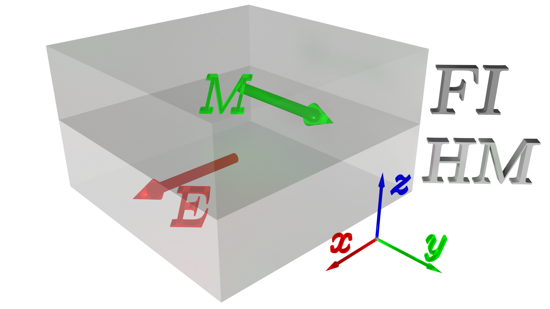
Figure 1: Schematic depiction of our system. The magnetization $M$ of the FI layer lies in the $+y$ direction, an electric field of magnitude $E$ is applied to the heavy metal layer (HM) in the $\pm x$ direction, and the interface between the layers lies in the $xy$ plane.

We describe the transfer of spin across the interface microscopically by the continuum-limit interaction Hamiltonian

$$H_{\mathrm{int}}=-\int\mathrm{d}^{3}\bm{r}\mathrm{d}^{3}\bm{r^{\prime}}\,J(\bm{r},\bm{r^{\prime}})\Big{[} b^{\dagger}(\bm{r^{\prime}})c^{\dagger}_{\downarrow}(\bm{r})c_{\uparrow}(\bm{r})$$

$$+b(\bm{r^{\prime}})c^{\dagger}_{\uparrow}(\bm{r})c_{\downarrow}(\bm{r})\Big{]},$$

where $c^{\dagger}_{\alpha}(\bm{r})$ [$c_{\alpha}(\bm{r})$] are fermionic creation [annihilation] operators of electrons with spin $\alpha\in\{\uparrow,\downarrow\}$ at position $\bm{r}$ in the HM, and $b^{\dagger}(\bm{r^{\prime}})$ [$b(\bm{r^{\prime}})$] is the bosonic creation [annihilation] operator of a circularly polarized Holstein-Primakoff magnon Holstein and Primakoff (1940) at position $\bm{r^{\prime}}$ inside the ferromagnet. We leave $J(\bm{r},\bm{r^{\prime}})$ to be some unknown coupling between the electrons and magnons, which is ultimately fixed by taking the classical limit Bender and Tserkovnyak (2015); Tserkovnyak et al. (2002).

Transforming to momentum space and using Fermi’s golden rule, we obtain the interfacial spin current $j_{\mathrm{s}}^{\text{int}}$, which can be expressed in terms of the real part of the spin mixing conductance per unit area $g_{\mathrm{r}}^{\uparrow\downarrow}$ as Bender et al. (2012); Bender and Tserkovnyak (2015)

$$j_{\mathrm{s}}^{\text{int}} =\frac{g^{\uparrow\downarrow}_{\mathrm{r}}}{\uppi s}\int\mathrm{d}\varepsilon\,g(\varepsilon)(\varepsilon-\Delta\mu)$$

$$\hskip 20.00003pt\times\left[n_{\mathrm{B}}\left(\frac{\varepsilon-\Delta\mu}{k_{\mathrm{B}}T_{\mathrm{e}}}\right)-n_{\mathrm{B}}\left(\frac{\varepsilon-\mu_{\mathrm{m}}}{k_{\mathrm{B}}T_{\mathrm{m}}}\right)\right].$$ (1)

(Similar expressions were derived by Takahashi et al. (2010) and Zhang and Zhang (2012a), although these are not given in terms of the spin-mixing conductance.)

Here, $s$ is the saturated spin density in the FI layer, $g(\varepsilon)$ is the magnon density of states, $n_{\mathrm{B}}\left(x\right)=\left[\mathrm{e}^{x}-1\right]^{-1}$ is the Bose-Einstein distribution function, $k_{\mathrm{B}}$ is Boltzmann’s constant, and $T_{\mathrm{m}}$ and $T_{\mathrm{e}}$ are the temperatures of the magnon and electron distributions, respectively, which we do not assume a priori to be equal (although the equal-temperature special case will be our primary interest). Of crucial importance in Eq. (1) are the magnon effective chemical potential $\mu_{\mathrm{m}}$—which we shall henceforth primarily refer to as the magnon spin accumulation—and the electron spin accumulation $\Delta\mu\equiv\mu^{\uparrow}-\mu^{\downarrow}$, which we define as the difference in chemical potentials for the spin-up and spin-down electrons. (In both cases, a positive accumulation means the majority of spin magnetic moments point in the $+y$ direction.)

We employ the magnon density of states

$$g(\varepsilon) =\frac{\sqrt{\varepsilon-\Delta}}{4\uppi^{2}J_{\mathrm{s}}^{\frac{3}{2}}}\Theta(\varepsilon-\Delta).$$

Here, $J_{\mathrm{s}}$ is the spin wave stiffness constant, $\Theta(x)$ is the Heaviside step function, and $\Delta$ is the magnon gap, caused by a combination of external magnetic fields and internal anisotropy fields in ferromagnetic materials Tang et al. (2016). In our primary analysis of a Pt|YIG bilayer, we take $\Delta\equiv\mu_{\mathrm{B}}\times$1\text{\,}\mathrm{T}$\approx k_{\mathrm{B}}\times$0.67\text{\,}\mathrm{K}$$ with $\mu_{\mathrm{B}}$ the Bohr magneton, in good agreement with e.g. Cherepanov et al. (1993), and in Sec. III.5 we specifically consider the limit of a vanishing magnon gap.

To treat the accumulations on equal footing, we now redefine $\mu_{\mathrm{m}}\to\delta\mu_{\mathrm{m}}$ and $\Delta\mu\to\delta\Delta\mu$, expand Eq. (1) to second order in $\delta$, and set $\delta=1$ to obtain

$$j_{\mathrm{s}}^{\text{int}}\simeq-\Bigg{[} k_{\mathrm{B}}T_{\mathrm{m}}I_{\mathrm{0}}+I_{\mathrm{e}}\Delta\mu+I_{\mathrm{m}}\mu_{\mathrm{m}}+\frac{I_{\mathrm{ee}}}{k_{\mathrm{B}}T_{\mathrm{e}}}(\Delta\mu)^{2}$$

$$+\frac{I_{\mathrm{mm}}}{k_{\mathrm{B}}T_{\mathrm{m}}}\mu_{\mathrm{m}}^{2}+\frac{I_{\mathrm{me}}}{k_{\mathrm{B}}T_{\mathrm{m}}}\mu_{\mathrm{m}}\Delta\mu\Bigg{]}\frac{g_{\mathrm{r}}^{\uparrow\downarrow}(k_{\mathrm{B}}T_{\mathrm{m}})^{\frac{3}{2}}}{4\uppi^{3}J_{\mathrm{s}}^{\frac{3}{2}}s}.$$ (2)

Here, the $I_{i}$ are dimensionless integrals given by Eqs. (7) in the Appendix. All $I_{i}$ are functions of $T_{\mathrm{m}}$ and $\Delta$, and $I_{0}$, $I_{\mathrm{e}}$ and $I_{\mathrm{ee}}$ additionally depend on $T_{\mathrm{e}}$. In the special case where $T_{\mathrm{m}}=T_{\mathrm{e}}$, $I_{0}$ vanishes, $I_{\mathrm{m}}=-I_{\mathrm{e}}$, and $I_{\mathrm{ee}}=-(I_{\mathrm{mm}}+I_{\mathrm{me}})$.

In addition to $j_{\mathrm{s}}^{\text{int}}$, the spin accumulations and the electric driving field $E$ give rise to the following spin currents in the $z$ direction:

$$j_{\mathrm{s}}^{\mathrm{e}} =\frac{\hbar}{2e}\left(-\frac{\sigma}{2e}\frac{\partial\Delta\mu}{\partial z}-\sigma\theta_{\mathrm{SH}}E\right),$$ (3a)

$$j_{\mathrm{s}}^{\mathrm{m}} =-\frac{\sigma_{\mathrm{m}}}{\hbar}\frac{\partial\mu_{\mathrm{m}}}{\partial z}.$$ (3b)

Here $j_{\mathrm{s}}^{\mathrm{e}}$ and $j_{\mathrm{s}}^{\mathrm{m}}$ are the electron and magnon spin currents, respectively. $\sigma$ is the electrical conductivity in the HM, $\sigma_{\mathrm{m}}$ is the magnon conductivity in the ferromagnet, $e$ is the elementary charge, and $\theta_{\mathrm{SH}}$ is the spin Hall angle.

In line with Cornelissen et al. (2016) and Zhang and Zhang (2012b), we assume the spin accumulations $\mu_{\mathrm{m}}$ and $\Delta\mu$ obey diffusion equations along the $z$-axis:

$$\frac{\mathrm{d}^{2}\mu_{\mathrm{m}}}{\mathrm{d}z^{2}} =\frac{\mu_{\mathrm{m}}}{l_{\mathrm{m}}^{2}}, \frac{\mathrm{d}^{2}\Delta\mu}{\mathrm{d}z^{2}} =\frac{\Delta\mu}{l_{\mathrm{e}}^{2}},$$

where $l_{\mathrm{m}}$ and $l_{\mathrm{e}}$ are the magnon and electron diffusion lengths, respectively. We solve these equations analytically subject to boundary conditions that demand continuity of the spin current across the interface and confinement of the currents to the sample:

$$j_{\mathrm{s}}^{\mathrm{m}}(0) =j_{\mathrm{s}}^{\mathrm{e}}(0)=j_{\mathrm{s}}^{\text{int}}(0),$$

$$j_{\mathrm{s}}^{\mathrm{m}}(L_{\mathrm{FI}}) =j_{\mathrm{s}}^{\mathrm{e}}(-L_{\mathrm{HM}})=0.$$

This system of equations now fully specifies the magnonic and electronic spin accumulations $\mu_{\mathrm{m}}$ and $\Delta\mu$, the latter of which enters the charge current $j_{\mathrm{c}}$ via the spin Hall effect:

$$j_{\mathrm{c}}(z) =\sigma E+\frac{\sigma\theta_{\mathrm{SH}}}{2e}\frac{\partial\Delta\mu(z)}{\partial z}.$$ (4)

The measured resistivity at some electric field strength $E$ is then given by the ratio of the electric field and the averaged charge current:

$$\rho(E) =\frac{E}{\frac{1}{L_{\mathrm{HM}}}\int_{-L_{\mathrm{HM}}}^{0}\mathrm{d}z\,j_{\mathrm{c}}(z)}.$$ (5)

Finally, we define the USMR $\mathcal{U}$ as the fractional difference in resistivity on inverting the electric field:

$$\mathcal{U} \equiv\left|\frac{\rho(E)-\rho(-E)}{\rho(E)}\right|=\left|1+\frac{\int_{-L_{\mathrm{HM}}}^{0}\mathrm{d}z\,j_{\mathrm{c}}(z;E)}{\int_{-L_{\mathrm{HM}}}^{0}\mathrm{d}z\,j_{\mathrm{c}}(z;-E)}\right|.$$

It should be noted that the even-ordered terms in the expansion of the interface current are vital to the appearance of unidrectional SMR. Suppose our system has equal magnon and electron temperature, such that the interfacial spin Seebeck term $I_{0}$ vanishes (see Section III.2), and we ignore the quadratic terms in Eq. (2). Then because the only term in the spin current equations (3) that is independent of the accumulations is $-\frac{\hbar\sigma\theta_{\mathrm{SH}}}{2e}E$ in Eq. (3a), we have that $\Delta\mu\propto\mu_{\mathrm{m}}\propto E$. Then by Eqs. (4) and (5), $j_{\mathrm{c}}\propto E$ and $\rho(E)\propto\frac{E}{E}$, such that $\mathcal{U}=0$. Conversely, with quadratic terms in the interfacial spin current, $\rho(E)\sim\frac{E}{E+E^{2}}$, and likewise if $I_{0}$ does not vanish, $\rho(E)\sim\frac{E}{1+E}$. Both cases give nonvanishing USMR. Physically, one can say that the spin-dependent electron and magnon populations couple together in a nonlinear fashion (namely, through the Bose-Einstein distributions in Eq. (1)), leading to a nonlinear dependence on the electric field.

III Results

III.1 Equal-temperature, finite gap case

Although our model can be solved analytically (up to evaluation of the integrals $I_{i}$), the full expression of $\mathcal{U}$ is unwieldy and therefore hardly insightful. To get an idea of the behavior of a real system, we use a set of parameters—listed in Table 1—corresponding to a Pt|YIG bilayer as a starting point. (Unless otherwise specified, all parameters used henceforth are to be taken from this table.)

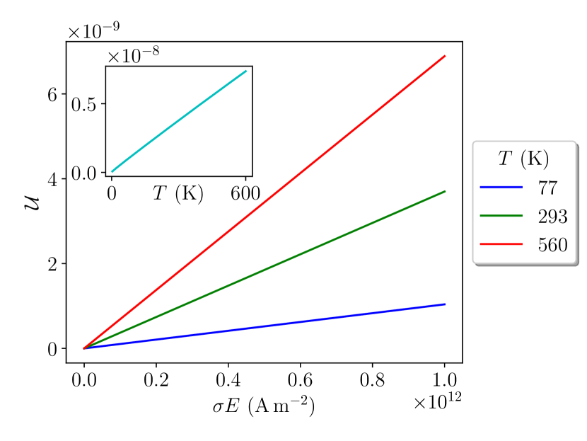
Figure 2: USMR $\mathcal{U}$ versus driving current $\sigma E$ for a Pt|YIG bilayer at liquid nitrogen temperature ($77\text{\,}\mathrm{K}$, blue), room temperature ($293\text{\,}\mathrm{K}$, green) and the YIG Curie temperature ($560\text{\,}\mathrm{K}$, red). Inset: USMR versus system temperature $T$ at fixed current $\sigma E=$1\text{\times}{10}^{12}\text{\,}\mathrm{A}\text{\,}{\mathrm{m}}^{-2}$$.

Fig. 2 shows the magnonic USMR of a Pt|YIG bilayer versus applied driving current ($\sigma E$) when $T_{\mathrm{m}}=T_{\mathrm{e}}=T$, at the temperature of liquid nitrogen ($77\text{\,}\mathrm{K}$, blue), room temperature ($293\text{\,}\mathrm{K}$, green) and the Curie temperature of YIG ($560\text{\,}\mathrm{K}$ Cherepanov et al. (1993), red). FI and HM layer thicknesses used are $90\text{\,}\mathrm{nm}$ and $3\text{\,}\mathrm{nm}$, respectively, in line with experimental measurements by Avci et al. (2015b).

In all cases the magnonic USMR is proportional to the applied electric current—that is, the cubic term found by Avci et al. (2018) is absent—and at room temperature has a value on the order of $10^{-9}$ at typical measurement currents Avci et al. (2015a). This is roughly four orders of magnitude weaker than the USMR obtained—both experimentally and theoretically—for FM|HM hybrids Avci et al. (2015a, b); Zhang and Vignale (2016); Yin et al. (2017), and is consistent with the experimental null results obtained for this system by Avci et al. (2015b). Note, however, that the thickness of the FI layer used by these authors is significantly lower than the magnon spin diffusion length $l_{\mathrm{m}}=$326\text{\,}\mathrm{nm}$$, which results in a suppressed USMR.

Furthermore, it can be seen in the inset of Fig. 2 that the magnonic USMR is, to good approximation, linear in the system temperature, in agreement with observations by Kim et al. (2016) and Avci et al. (2018).

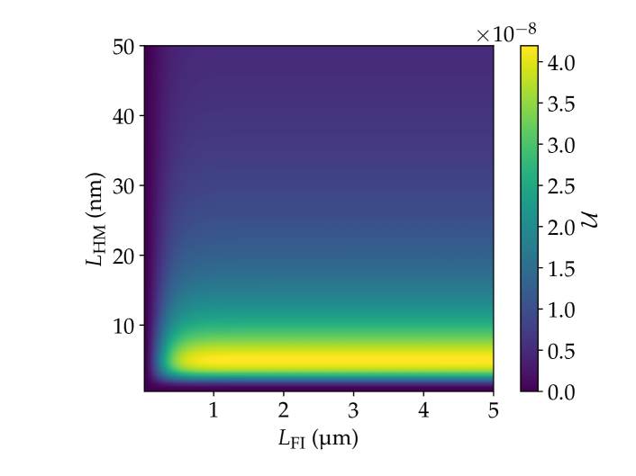
Figure 3: Pt|YIG USMR $\mathcal{U}$ at $T_{\mathrm{m}}=T_{\mathrm{e}}=$293\text{\,}\mathrm{K}$$ versus FI layer thickness $L_{\mathrm{FI}}$ and HM layer thickness $L_{\mathrm{HM}}$. A driving current $\sigma E=$1\text{\times}{10}^{12}\text{\,}\mathrm{A}\text{\,}{\mathrm{m}}^{-2}$$ is used. A maximal USMR of $4.2\text{\times}{10}^{-8}$ is reached at $L_{\mathrm{HM}}=$4.5\text{\,}\mathrm{nm}$$, $L_{\mathrm{FI}}=$5\text{\,}\mathrm{\SIUnitSymbolMicro m}$$.

In Fig. 3 we compute the USMR at $\sigma E=$1\text{\times}{10}^{12}\text{\,}\mathrm{A}\text{\,}{\mathrm{m}}^{-2}$$ as a function of both $L_{\mathrm{FI}}$ and $L_{\mathrm{HM}}$. A maximum is reached around $L_{\mathrm{HM}}\approx$4.5\text{\,}\mathrm{nm}$$, while in terms of $L_{\mathrm{FI}}$, a plateau is approached within a few spin diffusion lengths. By varying the layer thicknesses, a maximal USMR of $4.2\text{\times}{10}^{-8}$ can be achieved, an improvement of one order of magnitude compared to the thicknesses used by Avci et al. (2015b).

III.2 Thermal effects

We take into account a difference between the electron and magnon temperatures $T_{\mathrm{e}}$ and $T_{\mathrm{m}}$ by assuming these parameters are equal to the temperatures of the HM and FI layers, respectively, which we take to be homogeneous. We assume that the HM undergoes ohmic heating and dissipates this heat into the ferromagnet, which we take to be an infinite heat bath at temperature $T_{\mathrm{m}}$. We only take into account the interfacial (Kapitza) thermal resistance $R_{\mathrm{th}}$ between the HM and FI layers, leading to a simple expression for the HM temperature $T_{\mathrm{e}}$:

$$T_{\mathrm{e}} =T_{\mathrm{m}}+R_{\mathrm{th}}\sigma E^{2}L_{\mathrm{HM}}.$$

Using this model, we still find a linear dependence in the electric field, $\mathcal{U}\simeq u_{E}(T_{\mathrm{m}})\sigma E$, but the coefficient $u_{E}(T_{\mathrm{m}})$ increases by three orders of magnitude compared to the case where the electron and magnon temperatures are set to be equal. The overwhelming majority of this increase can be attributed to an interfacial spin Seebeck effect (SSE) Cornelissen et al. (2016); Schreier et al. (2013): it is caused by the accumulation-independent contribution $I_{0}$ (Eq. (7a)) in the interface current. When $I_{0}$ is artificially set to 0, $u_{E}(T_{\mathrm{m}})$ changes less than 1% from its equal-temperature value.

Furthermore, the overall magnitude of the interfacial SSE in our system can be attributed to the fact that we have a conductor|insulator interface: the current runs through the HM only, resulting in inhomogeneous Joule heating of the sample and a large temperature discontinuity across the interface.

III.3 Spin Hall angle

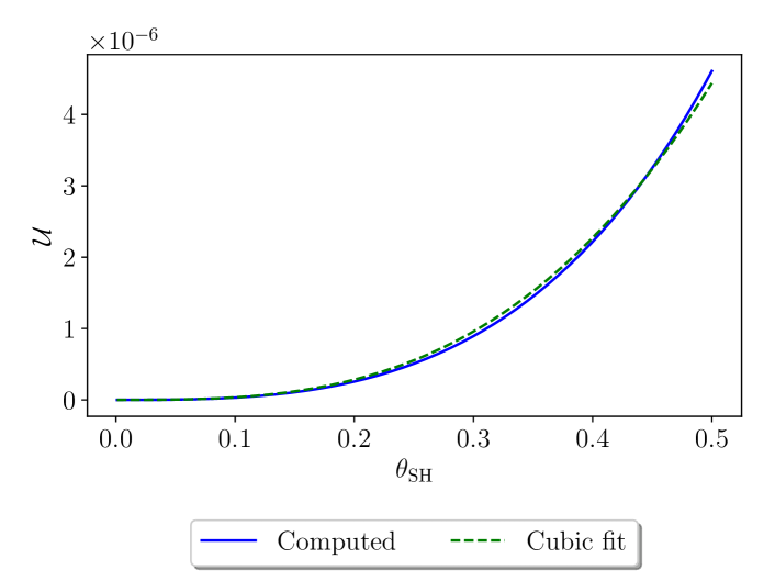
Figure 4: USMR $\mathcal{U}$ at $T_{\mathrm{m}}=T_{\mathrm{e}}=$293\text{\,}\mathrm{K}$$ versus spin Hall angle $\theta_{\mathrm{SH}}$. A driving current $\sigma E=$1\text{\times}{10}^{12}\text{\,}\mathrm{A}\text{\,}{\mathrm{m}}^{-2}$$ and FI and HM layer thicknesses $L_{\mathrm{FI}}=$5\text{\,}\mathrm{\SIUnitSymbolMicro m}$$ and $L_{\mathrm{HM}}=$4.5\text{\,}\mathrm{nm}$$ are used. Blue curve: computed value. Dashed green curve: fit of the form $\mathcal{U}=u_{\theta}\theta_{\mathrm{SH}}^{3}$, with $u_{\theta}\simeq$3.1\text{\times}{10}^{-4}$$.

The electronic spin accumulation $\Delta\mu$ at the interface in the standard spin Hall effect is linear in the electric field $E$ and spin Hall angle $\theta_{\mathrm{SH}}$ Chen et al. (2013). From the linearity in $E$, we may conclude that the terms in Eq. (2) that are linear in $\Delta\mu$ have a suppressed contribution to the USMR. Thus, the contribution of the interface current is of order $\theta_{\mathrm{SH}}^{2}$. Furthermore, $\Delta\mu$ enters the charge current (Eq. (4)) with a prefactor $\theta_{\mathrm{SH}}$, leaving the magnonic USMR predominantly cubic in the spin Hall angle. Indeed, in the special case $T_{\mathrm{m}}=T_{\mathrm{e}}$, expanding the full expression for $\mathcal{U}$ (which spans several pages and is therefore not reproduced within this work) in $\theta_{\mathrm{SH}}$ reveals that the first nonzero coefficient is that of $\theta_{\mathrm{SH}}^{3}$. This suggests a small change in $\theta_{\mathrm{SH}}$ potentially has a large effect on the USMR.

In Fig. 4 we plot the USMR for a Pt|YIG bilayer—once again using $T_{\mathrm{m}}=T_{\mathrm{e}}=$293\text{\,}\mathrm{K}$$—consisting of $4.5\text{\,}\mathrm{nm}$ of Pt and $5\text{\,}\mathrm{\SIUnitSymbolMicro m}$ of YIG, in which we sweep the spin Hall angle. Included is a cubic fit $\mathcal{U}=u_{\theta}\theta_{\mathrm{SH}}^{3}$, where we find $u_{\theta}\simeq$3.1\text{\times}{10}^{-4}$$. Here it can be seen that the magnonic USMR in HM|FI bilayers can, as expected, potentially acquire magnitudes roughly comparable to those in HM|FM systems, provided one can find or engineer a metal with a spin Hall angle several times greater than that of Pt. This suggests that very strong spin-orbit coupling (SOC) is liable to produce significant magnon-mediated USMR in FI|HM heterostructures, although we expect our model to break down in this regime.

III.4 A note on the magnon spin diffusion length

Although we use the analytic expression for the magnon spin diffusion lengthZhang and Zhang (2012b, a); Cornelissen et al. (2016),

$$l_{\mathrm{m}} =v_{\mathrm{th}}\sqrt{\frac{2}{3}\tau\tau_{\mathrm{mr}}}$$

—where $v_{\mathrm{th}}$ is the magnon thermal velocity, $\tau$ is the combined relaxation time, and $\tau_{\mathrm{mr}}$ is the magnonic relaxation time (see Table 1)—this is known to correspond poorly to reality, being at least an order of magnitude too low in the case of YIG Cornelissen et al. (2016). Artificially setting the magnon spin-diffusion length to the experimental value of $10\text{\,}\mathrm{\SIUnitSymbolMicro m}$ (while otherwise continuing to use the parameters from Table 1) results in a drop in USMR of some 4 orders of magnitude.

It follows directly that there exists some optimal value of $l_{\mathrm{m}}$ (which we shall label $l_{\mathrm{m,opt}}$) that maximizes the USMR, which we plot as a function of the FI layer thickness $L_{\mathrm{FI}}$ in Fig. 5, at $L_{\mathrm{HM}}=$4.5\text{\,}\mathrm{nm}$$ and $\sigma E=$1\text{\times}{10}^{12}\text{\,}\mathrm{A}\text{\,}{\mathrm{m}}^{-2}$$, and for various values of the magnon-phonon relaxation time $\tau_{\mathrm{mp}}$, which is the shortest and therefore most important timescale we take into account. For the physically realistic value of $\tau_{\mathrm{mp}}=$1\text{\,}\mathrm{ps}$$ (blue curve), the optimal magnon spin diffusion length is just $24\text{\,}\mathrm{nm}$. Although $l_{\mathrm{m,opt}}$ itself depends on $\tau_{\mathrm{mp}}$, the condition $l_{\mathrm{m}}=l_{\mathrm{m,opt}}$ acts to cancel the dependence of the USMR on the magnon-phonon relaxation time. Curiously, the USMR additionally loses its dependence on $L_{\mathrm{FI}}$, reaching a fixed value of $4.14\text{\times}{10}^{-7}$ for our parameters.

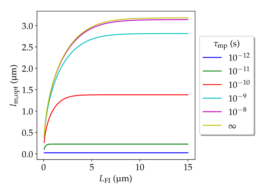
Figure 5: Value of the magnon spin diffusion length $l_{\mathrm{m}}$ that maximizes the USMR, as a function of FI layer thickness $L_{\mathrm{FI}}$, at various values of the magnon-phonon relaxation time $\tau_{\mathrm{mp}}$.

We further find that $l_{\mathrm{m,opt}}$ is independent of the spin Hall angle and driving current, and shows a weak decrease with increasing temperature provided the magnon-phonon scattering time is sufficiently short. A significant increase in the optimal spin diffusion length is only found at low temperatures and large $\tau_{\mathrm{mp}}$. Similarly, a weak dependence on the Gilbert damping constant $\alpha$ is found, becoming more significant at large $\tau_{\mathrm{mp}}$, with lower values of $\alpha$ corresponding to larger $l_{\mathrm{m,opt}}$. When $\alpha$ is swept, again the USMR at $l_{\mathrm{m}}=l_{\mathrm{m,opt}}$ acquires a universal value of $4.14\text{\times}{10}^{-7}$ for our system parameters.

III.5 Effect of the magnon gap

We have thus far utilised a fixed magnon gap with a value of $\Delta/\mu_{\mathrm{B}}=$1\text{\,}\mathrm{T}$$ for YIG. Although this is reasonable for typical systems, it is possible to significantly reduce the gap size by minimizing the anisotropy fields within the sample, e.g. using a combination of external fields Pini et al. (2005), optimized sample shapes Tang et al. (2016); Skarsvåg et al. (2015) and temperature Dillon (1957); Rodrigue et al. (1960). This leads us to consider the effect a decreased or even vanishing gap may have on our results.

Fig. 6 shows the USMR $\mathcal{U}$ for a Pt|YIG system ($4.5\text{\,}\mathrm{nm}$ of Pt and $5\text{\,}\mathrm{\SIUnitSymbolMicro m}$ of YIG) at room temperature, plotted against the driving current $\sigma E$, now for different values of the magnon gap $\Delta$. Here it can be seen that while $\mathcal{U}$ is linear in $E$ for large gap sizes and realistic currents, it shows limiting behavior at smaller gaps, becoming independent of the electric current above some threshold (provided one neglects the effect of Joule heating). At low current and intermediate magnon gap, the current dependence is nonlinear at $\mathcal{O}(I^{2})$ as opposed to the $\mathcal{O}(I^{3})$ behavior found by Avci et al. (2018).

Note also that the saturation value of the USMR is two to three orders of magnitude greater than the values found previously in our work, and of the same magnitude as the electronic contribution found by Zhang and Vignale (2016).

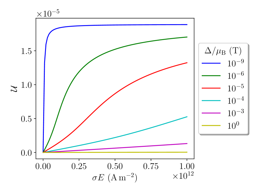
Figure 6: USMR $\mathcal{U}$ of a Pt($4.5\text{\,}\mathrm{nm}$)|YIG($5\text{\,}\mathrm{\SIUnitSymbolMicro m}$) bilayer at room temperature versus applied current $\sigma E$ at various values of the magnon gap $\Delta$. For large gaps, linear behavior is recovered at realistic currents, while for smaller gap sizes, the USMR saturates as the current is increased.

The maximal value of the USMR that can be achieved may be found by considering the full analytic expression for $\mathcal{U}$ in terms of the generic coefficients $I_{i}$ representing the dimensionless integrals given by Eqs. (7) in the Appendix. In the gapless limit $\Delta\to 0$ and at equal magnon and electron temperature ($T_{\mathrm{m}}=T_{\mathrm{e}}$), the second-order coefficients $I_{\mathrm{mm}}$ and $I_{\mathrm{me}}$ diverge, while their sum takes the constant value $\lambda\equiv I_{\mathrm{mm}}+I_{\mathrm{me}}\simeq 0.323551$ at room temperature. $I_{\mathrm{ee}}$ does not diverge, and obtains the value $-\lambda$.

Now working in the thick-ferromagnet limit ($L_{\mathrm{FI}}\to\infty$), we substitute $I_{\mathrm{me}}\to-I_{\mathrm{mm}}+\lambda$ and take the limits $E\to\infty$ and $I_{\mathrm{mm}}\to-\infty$. By application of l’Hôpital’s rule in the latter, all coefficients $I_{i}$ drop out of the expression for $\mathcal{U}$. This leaves only the asymptotic value, which, after expanding in $\theta_{\mathrm{SH}}$, reads

$$\mathcal{U}_{\text{max}}\! =\!\frac{4e^{2}l_{\mathrm{s}}^{2}\theta_{\mathrm{SH}}^{2}\sigma_{\mathrm{m}}\tanh^{2}\left(\!\frac{L_{\mathrm{HM}}}{2l_{\mathrm{s}}}\!\right)}{\hbar^{2}l_{\mathrm{m}}L_{\mathrm{HM}}\sigma\!+\!4l_{\mathrm{s}}e^{2}L_{\mathrm{HM}}\sigma_{\mathrm{m}}\coth\left(\!\frac{L_{\mathrm{HM}}}{l_{\mathrm{s}}}\!\right)}\!+\!\mathcal{O}(\theta_{\mathrm{SH}}^{4}).$$ (6)

Whereas the linear-in-$E$ regime of the magnonic USMR grows as $\theta_{\mathrm{SH}}^{3}$, we thus find that the leading-order behavior of the asymptotic value is only $\theta_{\mathrm{SH}}^{2}$, and the third-order term vanishes completely. Physically, this can be explained by the fact that the asymptotic magnonic USMR is purely a bulk effect: all details about the interface vanish, while parameters originating from the bulk spin- and charge currents remain. The appearance of $l_{\mathrm{m}}$ in the denominator and its absence in the numerator of Eq. (6) once again highlights that a large magnon spin diffusion length acts to suppress the USMR.

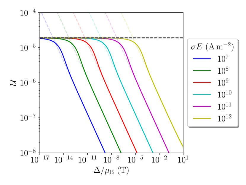
Figure 7: USMR $\mathcal{U}$ of a Pt($4.5\text{\,}\mathrm{nm}$)|YIG($5\text{\,}\mathrm{\SIUnitSymbolMicro m}$) bilayer at room temperature as function of the magnon gap size $\Delta$, for various values of the base charge current $\sigma E$. Note the log-log scaling. Solid colored lines: computed USMR. Dashed colored lines: continuations of the high-gap tails of the corresponding curves according to the one-parameter fit $\mathcal{U}=u_{0}/\sqrt{\Delta}$. Dashed black line: asymptotic value of the USMR as given by Eq. (6).

Fig. 7 is a log-log plot of the USMR versus gap size $\Delta$ at various values of the driving current $\sigma E$. Here the value $\mathcal{U}_{\text{max}}$ is shown as a dashed black line, indicating that this is indeed the value to which $\mathcal{U}$ converges in the gapless limit or at high current. Moreover, it shows that for given $\sigma E$, one can find a turning point at which the USMR switches relatively abruptly from being nearly constant to decreasing as $1/\sqrt{\Delta}$.

A (backwards) continuation of the decreasing tails is included in Fig. 7 as dashed lines following the one-parameter fit $\mathcal{U}=u_{0}/\sqrt{\Delta}$, and we define the threshold gap $\Delta_{\mathrm{th}}$ as the value of $\Delta$ where this continuation intersects $\mathcal{U}_{\text{max}}$. We then find that $\Delta_{\mathrm{th}}$ scales as $E^{2}$, or conversely, that the driving current required to saturate the USMR scales as the square root of the magnon gap.

We note that although the small-gap regime is mathematically valid (even in the limit $\Delta\to 0$, as $\Delta$ may be brought arbitrarily close to 0 in a continuous manner), it does not necessarily correspond to a physical situation: when the anisotropy vanishes, the magnetization of the FI layer may be reoriented freely, which will break our initial assumptions. Nevertheless, in taking the gapless limit, we are able to predict an upper limit on the magnonic USMR.

IV Conclusions

Using a simple drift-diffusion model, we have shown that magnonic spin accumulation near the interface between a ferromagnetic insulator and a heavy metal leads to a small but nonvanishing contribution to the unidirectional spin Hall magnetoresistance of FI|HM heterostructures. Central to our model is an interfacial spin current originating from a spin-flip scattering process whereby electrons in the heavy metal create or annihilate magnons in the ferromagnet. This current is markedly nonlinear in the electronic and magnonic spin accumulations at the interface, and it is exactly this nonlinearity which gives rise to the magnonic USMR.

For Pt|YIG bilayers, we predict that the magnonic USMR $\mathcal{U}$ is at most on the order of $10^{-8}$, roughly three orders of magnitude weaker than the measured USMR in FM|HM hybrids (where electronic spin accumulation is thought to form the largest contribution). This is fully consistent with experiments that fail to detect USMR in Pt|YIG systems, as the tiny signal is drowned out by the interfacial spin Seebeck effect, which has a similar experimental signature and is enhanced compared to the FM|HM case due to inhomogeneous Joule heating.

We have shown that the magnon-mediated USMR is approximately cubic in the spin Hall angle of the metal, suggesting that metals with extremely large spin Hall angles may provide a significantly larger USMR than Pt. It is therefore plausible that a large magnonic USMR can exist in systems with very strong spin-orbit coupling, even though our model would break down in this regime.

The magnonic USMR depends strongly on the magnon spin diffusion length $l_{\mathrm{m}}$ in the ferromagnet. Motivated by a large discrepancy between experimental values and theoretical predictions of $l_{\mathrm{m}}$, we have shown that a significant increase in USMR can be realized if a method is found to engineer this parameter to specific, optimal values that, for realistic values of the magnon-phonon relaxation time $\tau_{\mathrm{mp}}$ (on the order of $1\text{\,}\mathrm{ps}$ for YIG), are significantly shorter than those measured experimentally or computed theoretically. We further find that when the magnon spin diffusion length has its optimal value, the USMR becomes independent of the ferromagnet’s thickness and Gilbert damping constant.

Although in physically reasonable regimes, the magnonic USMR is to very good approximation linear in the applied driving current $\sigma E$, it saturates to a fixed value given extremely large currents or a strongly reduced magnon gap $\Delta$. The transition from linear to constant behavior in the driving current is heralded by a turning point which is proportional to the square root of the magnon gap. The asymptotic behavior of the USMR beyond the turning point is governed by the bulk spin- and charge currents, and is completely independent of the details of the interface.

While a vast reduction in $\Delta$ is required to bring the saturation current of a Pt|YIG bilayer within experimentally reasonable regimes, the magnonic USMR scales as $1/\sqrt{\Delta}$ at currents below the turning point, suggesting that highly isotropic FI|HM samples are most likely to produce a measurable magnonic USMR. The increase in magnonic USMR at low gaps (and large currents) is in good qualitative agreement with the recent experimental work of Avci et al. (2018), as is the linear dependence on system temperature.

A notable disagreement with the experimental data of Avci et al. (2018) is found in the scaling of the current dependence, which in our results lacks an $\mathcal{O}(I^{3})$ term at large magnon gaps and contains an $\mathcal{O}(I^{2})$ term at intermediate gaps. It is still unclear whether this discrepancy can be explained by system differences, such as the finite electrical resistance of Co or the presence of Joule heating.

Finally, we note that while our results apply to ferromagnetic insulators, it is reasonable to assume a magnonic contribution also exists in HM|FM heterostructures, although the possibility of coupled transport of magnons and electrons makes such systems more difficult to model. Additionally, various extensions of our model may be considered, such as the incorporation of spin-momentum locking Yasuda et al. (2016), ellipticity of magnons, heat transport and nonuniform temperature profiles Cornelissen et al. (2016), directional dependence of the magnetization, etc.

V Acknowledgements

R.A.D. is member of the D-ITP consortium, a program of the Dutch Organisation for Scientific Research (NWO) that is funded by the Dutch Ministry of Education, Culture and Science (OCW). This work is funded by the European Research Council (ERC).

Description	Symbol	Expression	Value at $T=$293\text{\,}\mathrm{K}$$	Ref.
YIG spin-wave stiffness constant	$J_{\mathrm{s}}$		$8.458\text{\times}{10}^{-40}\text{\,}\mathrm{J}\text{\,}{\mathrm{m}}^{2}$	Cornelissen et al. (2016)
YIG spin quantum number per unit cell	$S$		10	Cornelissen et al. (2016)
YIG lattice constant	$a$		$1.2376\text{\,}\mathrm{nm}$	Cornelissen et al. (2016)
YIG Gilbert damping constant	$\alpha$		$1\text{\times}{10}^{-4}$	Cornelissen et al. (2016)
YIG spin number density	$s$	$Sa^{-3}$	$5.2754\text{\times}{10}^{27}\text{\,}{\mathrm{m}}^{-3}$	Cornelissen et al. (2016)
YIG magnon gap	$\Delta$		$9.3\text{\times}{10}^{-24}\text{\,}\mathrm{J}$	Cherepanov et al. (1993)
YIG magnon-phonon scattering time	$\tau_{\mathrm{mp}}$		$1\text{\,}\mathrm{ps}$	Cornelissen et al. (2016)
YIG magnon relaxation time	$\tau_{\mathrm{mr}}$	$\frac{\hbar}{2\alpha k_{\mathrm{B}}T_{\mathrm{m}}}$	$130\text{\,}\mathrm{ps}$	Cornelissen et al. (2016)
Combined magnon relaxation time	$\tau$	$\left(\frac{1}{\tau_{\mathrm{mr}}}+\frac{1}{\tau_{\mathrm{mp}}}\right)^{-1}$	$1\text{\,}\mathrm{ps}$	Cornelissen et al. (2016)
Magnon thermal de Broglie wavelength	$\Lambda$	$\sqrt{\frac{4\uppi J_{\mathrm{s}}}{k_{\mathrm{B}}T_{\mathrm{m}}}}$	$1.62\text{\,}\mathrm{nm}$	Cornelissen et al. (2016)
Magnon thermal velocity	$v_{\mathrm{th}}$	$\frac{2\sqrt{J_{\mathrm{s}}k_{\mathrm{B}}T}}{\hbar}$	$35.1\text{\,}\mathrm{km}\text{\,}{\mathrm{s}}^{-1}$	Cornelissen et al. (2016)
Magnon spin diffusion length	$l_{\mathrm{m}}$	$v_{\mathrm{th}}\sqrt{\frac{2}{3}\tau\tau_{\mathrm{mr}}}$	$326\text{\,}\mathrm{nm}$	Cornelissen et al. (2016)
Magnon spin conductivity	$\sigma_{\mathrm{m}}$	$\zeta\left(\frac{3}{2}\right)^{2}\frac{J_{\mathrm{s}}}{\Lambda^{3}}\tau$	$1.35\text{\times}{10}^{-24}\text{\,}\mathrm{J}\text{\,}\mathrm{s}\text{\,}{\mathrm{m}}^{-1}$	Cornelissen et al. (2016)
Real part of spin-mixing conductance	$g_{\mathrm{r}}^{\uparrow\downarrow}$		$5\text{\times}{10}^{18}\text{\,}{\mathrm{m}}^{-2}$	Bender et al. (2012)
Pt electrical conductivity	$\sigma$		$1\text{\times}{10}^{7}\text{\,}\mathrm{S}\text{\,}{\mathrm{m}}^{-1}$	ASM Handbook Committee (1990)
Pt spin Hall angle	$\theta_{\mathrm{SH}}$		0.11	Cornelissen et al. (2016)
Pt electron diffusion length	$l_{\mathrm{s}}$		$1.5\text{\,}\mathrm{nm}$	Cornelissen et al. (2016)
Pt|YIG Kapitza resistance	$R_{\mathrm{th}}$		$3.58\text{\times}{10}^{-9}\text{\,}{\mathrm{m}}^{2}\text{\,}\mathrm{K}\text{\,}{\mathrm{W}}^{-1}$	Schreier et al. (2013)

Table 1: System parameters for a Pt|YIG bilayer film.

*

Appendix A Interfacial spin current integrals

The following dimensionless integrals appear in the second-order expansion of the interfacial spin current to the spin accumulations, Eq. (2):

$$I_{\mathrm{0}} =\int_{\frac{\Delta}{k_{\mathrm{B}}T_{\mathrm{m}}}}^{\infty}\mathrm{d}x\,\sqrt{x-\frac{\Delta}{k_{\mathrm{B}}T_{\mathrm{m}}}}x\left(n_{\mathrm{B}}\left(x\right)-n_{\mathrm{B}}\left(\frac{T_{\mathrm{m}}}{T_{\mathrm{e}}}x\right)\right),$$ (7a)

$$I_{\mathrm{e}} =\int_{\frac{\Delta}{k_{\mathrm{B}}T_{\mathrm{m}}}}^{\infty}\mathrm{d}x\,\sqrt{x-\frac{\Delta}{k_{\mathrm{B}}T_{\mathrm{m}}}}\left(n_{\mathrm{B}}\left(\frac{T_{\mathrm{m}}}{T_{\mathrm{e}}}x\right)-n_{\mathrm{B}}\left(x\right)-\frac{T_{\mathrm{m}}}{T_{\mathrm{e}}}x\mathrm{e}^{\frac{T_{\mathrm{m}}}{T_{\mathrm{e}}}x}\left[n_{\mathrm{B}}\left(\frac{T_{\mathrm{m}}}{T_{\mathrm{e}}}x\right)\right]^{2}\right),$$ (7b)

$$I_{\mathrm{m}} =\int_{\frac{\Delta}{k_{\mathrm{B}}T_{\mathrm{m}}}}^{\infty}\mathrm{d}x\,\sqrt{x-\frac{\Delta}{k_{\mathrm{B}}T_{\mathrm{m}}}}x\mathrm{e}^{x}\left[n_{\mathrm{B}}\left(x\right)\right]^{2},$$ (7c)

$$I_{\mathrm{ee}} =\int_{\frac{\Delta}{k_{\mathrm{B}}T_{\mathrm{m}}}}^{\infty}\mathrm{d}x\,\sqrt{x-\frac{\Delta}{k_{\mathrm{B}}T_{\mathrm{m}}}}\left(\mathrm{e}^{\frac{T_{\mathrm{m}}}{T_{\mathrm{e}}}x}\left[n_{\mathrm{B}}\left(\frac{T_{\mathrm{m}}}{T_{\mathrm{e}}}x\right)\right]^{3}\left[\mathrm{e}^{\frac{T_{\mathrm{m}}}{T_{\mathrm{e}}}x}-1-\frac{T_{\mathrm{m}}x}{2T_{\mathrm{e}}}\left(\mathrm{e}^{\frac{T_{\mathrm{m}}}{T_{\mathrm{e}}}x}+1\right)\right]\right),$$ (7d)

$$I_{\mathrm{mm}} =\int_{\frac{\Delta}{k_{\mathrm{B}}T_{\mathrm{m}}}}^{\infty}\mathrm{d}x\,\sqrt{x-\frac{\Delta}{k_{\mathrm{B}}T_{\mathrm{m}}}}\frac{x}{2}\mathrm{e}^{x}\left[\mathrm{e}^{x}+1\right]\left[n_{\mathrm{B}}\left(x\right)\right]^{3},$$ (7e)

$$I_{\mathrm{me}} =-\int_{\frac{\Delta}{k_{\mathrm{B}}T_{\mathrm{m}}}}^{\infty}\mathrm{d}x\,\sqrt{x-\frac{\Delta}{k_{\mathrm{B}}T_{\mathrm{m}}}}\mathrm{e}^{x}\left[n_{\mathrm{B}}\left(x\right)\right]^{2}.$$ (7f)

References

- McGuire and Potter (1975) T. McGuire and R. Potter, IEEE Transactions on Magnetics 11, 1018 (1975).
- Binasch et al. (1989) G. Binasch, P. Grünberg, F. Saurenbach, and W. Zinn, Physical Review B 39, 4828 (1989).
- Chen et al. (2013) Y.-T. Chen, S. Takahashi, H. Nakayama, M. Althammer, S. T. B. Goennenwein, E. Saitoh, and G. E. W. Bauer, Physical Review B 87, 144411 (2013), arXiv:1302.1352 [cond-mat.mes-hall] .
- Avci et al. (2015a) C. O. Avci, K. Garello, A. Ghosh, M. Gabureac, S. F. Alvarado, and P. Gambardella, Nature Physics 11, 570 (2015a), arXiv:1502.06898 [cond-mat.mes-hall] .
- Yasuda et al. (2016) K. Yasuda, A. Tsukazaki, R. Yoshimi, K. S. Takahashi, M. Kawasaki, and Y. Tokura, Physical Review Letters 117, 127202 (2016), arXiv:1609.05906 [cond-mat.mtrl-sci] .
- Yin et al. (2017) Y. Yin, D.-S. Han, M. C. H. de Jong, R. Lavrijsen, R. A. Duine, H. J. M. Swagten, and B. Koopmans, Applied Physics Letters 111, 232405 (2017), arXiv:1711.06488 [cond-mat.mtrl-sci] .
- Avci et al. (2017) C. O. Avci, M. Mann, A. J. Tan, P. Gambardella, and G. S. D. Beach, Applied Physics Letters 110, 203506 (2017).
- Zhang and Vignale (2016) S. S.-L. Zhang and G. Vignale, Physical Review B 94, 140411 (2016), arXiv:1608.02124 [cond-mat.mes-hall] .
- Kim et al. (2016) K. J. Kim, T. Moriyama, T. Koyama, D. Chiba, S. W. Lee, S. J. Lee, K. J. Lee, H. W. Lee, and T. Ono, ArXiv e-prints (2016), arXiv:1603.08746 [cond-mat.mtrl-sci] .
- Avci et al. (2018) C. O. Avci, J. Mendil, G. S. D. Beach, and P. Gambardella, Physical Review Letters 121, 087207 (2018).
- Chudnovsky (2007) E. M. Chudnovsky, Physical Review Letters 99, 206601 (2007), arXiv:0709.0725 [cond-mat.mes-hall] .
- Zhang et al. (2015) W. Zhang, W. Han, X. Jiang, S.-H. Yang, and S. S. P. Parkin, Nature Physics 11, 496 (2015), arXiv:1504.07929 [cond-mat.mes-hall] .
- Holstein and Primakoff (1940) T. Holstein and H. Primakoff, Physical Review 58, 1098 (1940).
- Bender and Tserkovnyak (2015) S. A. Bender and Y. Tserkovnyak, Physical Review B 91, 140402 (2015), arXiv:1409.7128 [cond-mat.mes-hall] .
- Tserkovnyak et al. (2002) Y. Tserkovnyak, A. Brataas, and G. E. Bauer, Physical Review Letters 88, 117601 (2002), cond-mat/0110247 .
- Bender et al. (2012) S. A. Bender, R. A. Duine, and Y. Tserkovnyak, Physical Review Letters 108, 246601 (2012), arXiv:1111.2382 [cond-mat.mes-hall] .
- Takahashi et al. (2010) S. Takahashi, E. Saitoh, and S. Maekawa, in Journal of Physics Conference Series, Journal of Physics Conference Series, Vol. 200 (IOP Publishing, 2010) p. 062030.
- Zhang and Zhang (2012a) S. S.-L. Zhang and S. Zhang, Physical Review B 86, 214424 (2012a), arXiv:1210.2735 [cond-mat.mes-hall] .
- Tang et al. (2016) C. Tang, M. Aldosary, Z. Jiang, H. Chang, B. Madon, K. Chan, M. Wu, J. E. Garay, and J. Shi, Applied Physics Letters 108, 102403 (2016).
- Cherepanov et al. (1993) V. Cherepanov, I. Kolokolov, and V. L’vov, Physics Reports 229, 81 (1993).
- Cornelissen et al. (2016) L. J. Cornelissen, K. J. H. Peters, G. E. W. Bauer, R. A. Duine, and B. J. van Wees, Physical Review B 94, 014412 (2016), arXiv:1604.03706 [cond-mat.mes-hall] .
- Zhang and Zhang (2012b) S. S.-L. Zhang and S. Zhang, Physical Review Letters 109, 096603 (2012b), arXiv:1208.5812 [cond-mat.mes-hall] .
- Avci et al. (2015b) C. O. Avci, K. Garello, J. Mendil, A. Ghosh, N. Blasakis, M. Gabureac, M. Trassin, M. Fiebig, and P. Gambardella, Applied Physics Letters 107, 192405 (2015b).
- Schreier et al. (2013) M. Schreier, A. Kamra, M. Weiler, J. Xiao, G. E. W. Bauer, R. Gross, and S. T. B. Goennenwein, Physical Review B 88, 094410 (2013), arXiv:1306.4292 [cond-mat.mes-hall] .
- Pini et al. (2005) M. G. Pini, P. Politi, and R. L. Stamps, Physical Review B 72, 014454 (2005), cond-mat/0503538 .
- Skarsvåg et al. (2015) H. Skarsvåg, C. Holmqvist, and A. Brataas, Physical Review Letters 115, 237201 (2015), arXiv:1506.06029 [cond-mat.mes-hall] .
- Dillon (1957) J. F. Dillon, Physical Review 105, 759 (1957).
- Rodrigue et al. (1960) G. P. Rodrigue, H. Meyer, and R. V. Jones, Journal of Applied Physics 31, S376 (1960).
- ASM Handbook Committee (1990) ASM Handbook Committee, ASM handbook, Vol. 2 (ASM International, Materials Park, Ohio, 1990).