Numerical study of the $\mathcal{N}=2$ Landau–Ginzburg model with two superfields

Abstract

In the low energy limit, the two-dimensional massless $\mathcal{N}=2$ Wess–Zumino (WZ) model with a quasi-homogeneous superpotential is believed to become a superconformal field theory. This conjecture of the Landau–Ginzburg (LG) description has been studied numerically in the case of the $A_{2}$, $A_{3}$, and $E_{6}$ minimal models. In this paper, by using a supersymmetric-invariant non-perturbative formulation, we simulate the WZ model with two superfields corresponding to the $D_{3}$, $D_{4}$, and $E_{7}$ models. Then, we numerically determine the central charge, and obtain the results that are consistent with the conjectured correspondence. We hope that this numerical approach, when further developed, will be useful to investigate superstring theory via the LG/Calabi–Yau correspondence.

B16, B24, B34

1 Introduction

At an extremely low-energy scale, the two-dimensional massless $\mathcal{N}=2$ Wess–Zumino (WZ) model Wess:1974tw with a quasi-homogeneous superpotential is believed to become an $\mathcal{N}=2$ superconformal field theory (SCFT). This conjecture of the Landau–Ginzburg (LG) description has been studied from various aspects DiVecchia:1985ief ; DiVecchia:1986cdz ; DiVecchia:1986fwg ; Boucher:1986bh ; Gepner:1986ip ; Cappelli:1986hf ; Cappelli:1986ed ; Gepner:1986hr ; Gepner:1987qi ; Cappelli:1987xt ; Kato:1987td ; Gepner:1987vz ; Kastor:1988ef ; Vafa:1988uu ; Martinec:1988zu ; Lerche:1989uy ; Howe:1989qr ; Cecotti:1989jc ; Howe:1989az ; Cecotti:1989gv ; Cecotti:1990kz ; Witten:1993jg . However, we have no complete proof of this conjecture. It is difficult to prove because the coupling constant becomes strong at the low-energy region and the perturbative theory possesses infrared (IR) divergences; the LG description is a truly non-perturbative phenomenon. An interesting approach to this issue may be a numerical and non-perturbative technique on the basis of the lattice field theory.

By using such numerical approaches, the $A_{2}$ and $A_{3}$ minimal models were simulated in Refs. Kawai:2010yj ; Kamata:2011fr ; Morikawa:2018ops , where superpotentials in the corresponding WZ model are given as the cubic and quartic ones containing a single superfield; see Table 1 Vafa:1988uu . These studies are based on either a lattice formulation in Ref. Kikukawa:2002as , or a supersymmetry-preserving formulation with a momentum cutoff in Ref. Kadoh:2009sp ; both non-perturbative formulations make essential use of the existence of the Nicolai map Nicolai:1979nr ; Nicolai:1980jc ; Parisi:1982ud ; Cecotti:1983up . In above numerical studies, their results of the scaling dimension and the central charge are consistent with the expected values in the $A_{2}$ and $A_{3}$ minimal models within numerical errors. Therefore, we have now numerical evidences for the LG/SCFT correspondence in the case of the $A_{2}$, $A_{3}$, and $E_{6}$ ($\cong A_{2}\otimes A_{3}$) minimal models.

Table 1: ADE classification

Algebra	Superpotential $W$	Central charge $c$
$A_{n}$	$\Phi^{n+1}$, $n\geqq 1$	$3-6/(n+1)$
$D_{n}$	$\Phi^{n-1}+\Phi\Phi^{\prime 2}$, $n\geqq 3$	$3-6/2(n-1)$
$E_{6}$	$\Phi^{3}+\Phi^{\prime 4}$	$3-6/12$
$E_{7}$	$\Phi^{3}+\Phi\Phi^{\prime 3}$	$3-6/18$
$E_{8}$	$\Phi^{3}+\Phi^{\prime 5}$	$3-6/30$

In this paper, on the basis of the momentum cutoff regularization Kadoh:2009sp and the analysis in Ref. Morikawa:2018ops , we simulate the two-dimensional $\mathcal{N}=2$ WZ model corresponding to $D$- and $E$-type theories. The method in Ref. Morikawa:2018ops is generalized to the WZ model with multiple superfields and more complicated superpotentials. Then, from an IR behavior of the energy-momentum tensor (EMT), we numerically determine the central charge of the $D_{3}$, $D_{4}$, and $E_{7}$ models; we obtain the results that are consistent with the conjectured correspondence. We also measure the “effective central charge” Kamata:2011fr ; Morikawa:2018ops , which is analogous to the Zamolodchikov’s $c$-function Zamolodchikov:1986gt ; Cappelli:1989yu . Although the theoretical background of the formulation is not completely obvious so far, our computational results support the validity of the formulation even if we consider multi-superfield theories. We hope to apply this approach to some models which is neither a minimal model nor a product of minimal models (Gepner model Gepner:1987qi ; Gepner:1987vz ), and then develop a numerical method to investigate superstring theory via the LG/Calabi–Yau correspondence Martinec:1988zu ; Cecotti:1990wz ; Greene:1988ut ; Witten:1993yc .

2 Nicolai mapping for the multi-superfield WZ model

Our numerical simulation is based on the formulation in Ref. Kadoh:2009sp . The detailed discussions for the formulation are given in Ref. Morikawa:2018ops . These preceding studies treat the two-dimensional $\mathcal{N}=2$ WZ model with a single superfield. In this section, we summarize basic formulas of the formulation for the WZ model with multiple superfields.

Suppose that the system is defined in a two-dimensional Euclidean physical box $L_{0}\times L_{1}$. In what follows, we work in the momentum space with an ultraviolet (UV) cutoff,

$$p_{\mu}=\frac{2\pi}{L_{\mu}}n_{\mu}\qquad\left(n_{\mu}=0,\pm 1,\pm 2,\dots,\pm\frac{L_{\mu}}{2a}\right),$$ (2.1)

where the Greek index $\mu$ runs over $0$ and $1$, and repeated indices are not summed over; $L_{\mu}/a$ is taken as even integers, and $a$ is a unit of dimensionful quantities. A limit $a\to 0$ removes the UV cutoff, being similar to the continuum limit. In fact, when we take $L_{\mu}/a$ as odd integers, the unit $a$ itself is the lattice spacing in the dimensional reduction of the four-dimensional lattice formulation Bartels:1983wm based on the SLAC derivative Drell:1976bq ; Drell:1976mj .

It is well recognized that the regularization based on the SLAC derivative violates the locality. The four-dimensional SLAC derivative is plagued by the pathology that the locality of the theory is not automatically restored in the continuum limit Dondi:1976tx ; Karsten:1979wh ; Kato:2008sp ; Bergner:2009vg . In the two- or three-dimensional case, on the other hand, one can argue the restoration of the locality in the continuum limit within perturbation theory for massive WZ models Kadoh:2009sp . For massless models, it is not clear whether the restoration is automatically accomplished because perturbation techniques are hindered by the IR divergences. We believe that the numerical results in Refs. Kamata:2011fr ; Morikawa:2018ops and ours below support the validity of the formulation.

For simplicity, we set $a=1$. We basically use the complex coordinates for the momentum, $p_{z}=(p_{0}-ip_{1})/2$ and $p_{\bar{z}}=(p_{0}+ip_{1})/2$. In general, the two-dimensional $\mathcal{N}=2$ WZ model contains $N_{\Phi}$ superfields, $\{\Phi_{I}\}_{I=1,\dots,N_{\Phi}}$. A supermultiplet $\Phi_{I}$ consists of a complex scalar $A_{I}$, left- and right-handed spinors $(\psi_{I},\bar{\psi}_{I})$, and a complex auxiliary field $F_{I}$. Then, the action of the two-dimensional $\mathcal{N}=2$ WZ model with a quasi-homogeneous superpotential $W(\{A\})$ is given by

$$S =\frac{1}{L_{0}L_{1}}\sum_{p}\sum_{I}\Biggl{[}4p_{z}A_{I}^{*}(-p)p_{\bar{z}}A_{I}(p)-F_{I}^{*}(-p)F_{I}(p)$$

$$\qquad\qquad\qquad\qquad-F_{I}(-p)\frac{\partial W(\{A\})}{\partial A_{I}}(p)-F_{I}^{*}(-p)\frac{\partial W(\{A\})^{*}}{\partial A_{I}^{*}}(p)$$

$$\qquad\qquad\qquad\qquad+(\bar{\psi}_{\dot{1}},\psi_{2})_{I}(-p)\sum_{J}\begin{pmatrix}2\delta_{IJ}p_{z}&\frac{\partial^{2}W(\{A\})^{*}}{\partial A_{I}^{*}\partial A_{J}^{*}}*\\ \frac{\partial^{2}W(\{A\})}{\partial A_{I}\partial A_{J}}*&2\delta_{IJ}p_{\bar{z}}\end{pmatrix}\begin{pmatrix}\psi_{1}\\ \bar{\psi}_{\dot{2}}\end{pmatrix}_{J}(p)\Biggr{]},$$ (2.2)

where $*$ denotes the convolution

$$(\varphi_{1}*\varphi_{2})(p)\equiv\frac{1}{L_{0}L_{1}}\sum_{q}\varphi_{1}(q)\varphi_{2}(p-q).$$ (2.3)

The field products in $\partial W(\{A\})/\partial A_{I}$ and $\partial W(\{A\})/\partial A_{I}\partial A_{J}$ are understood as this convolution. Integrating over the auxiliary fields $\{F\}$, we obtain the action in terms of the physical component fields,

$$S =S_{B}+\frac{1}{L_{0}L_{1}}\sum_{p}\sum_{I,J}(\bar{\psi}_{\dot{1}},\psi_{2})_{I}(-p)\begin{pmatrix}2i\delta_{IJ}p_{z}&\frac{\partial^{2}W(\{A\})^{*}}{\partial A_{I}^{*}\partial A_{J}^{*}}*\\ \frac{\partial^{2}W(\{A\})}{\partial A_{I}\partial A_{J}}*&2i\delta_{IJ}p_{\bar{z}}\end{pmatrix}\begin{pmatrix}\psi_{1}\\ \bar{\psi}_{\dot{2}}\end{pmatrix}_{J}(p),$$ (2.4)

where $S_{B}$ is the bosonic part of the total action

$$S_{B} =\frac{1}{L_{0}L_{1}}\sum_{p}\sum_{I}N_{I}^{*}(-p)N_{I}(p), N_{I}(p) =2p_{z}A_{I}(p)+\frac{\partial W(\{A\})^{*}}{\partial A_{I}^{*}}(p).$$ (2.5)

The new variables $\{N\}$ (2.5) specify the so-called Nicolai map Nicolai:1979nr ; Nicolai:1980jc ; Parisi:1982ud ; Cecotti:1983up , the change of variables from $\{A\}$ to $\{N\}$. This mapping simplifies the path-integral weight drastically; the partition function where the fermion fields are integrated is given by

$$\mathcal{Z} =\int\prod_{|p_{\mu}|\leq\pi}\prod_{I}[dN_{I}(p)dN_{I}^{*}(p)]\,e^{-S_{B}}\sum_{k}\left.\operatorname{sign}\det\frac{\partial(\{N\},\{N^{*}\})}{\partial(\{A\},\{A^{*}\})}\right|_{\{A\}=\{A\}_{k}},$$ (2.6)

where $\{A\}_{k}$ ($k=1$, $2$, …) is a set of solutions of the equation

$$2ip_{z}A_{I}(p)+\frac{\partial W(\{A\})^{*}}{\partial A_{I}^{*}}(p)-N_{I}(p)=0.$$ (2.7)

The weight $\exp(-S_{B})$ is a Gaussian function of the variables $\{N\}$. All we should do to obtain configurations of $\{N\}$ and $\{A\}$ is the following: We generate complex random numbers $\{N(p)\}$ from the Gaussian distribution for each momentum, and then, solve numerically the algebraic equation (2.7) with respect to $\{A\}$. Note that, however, our numerical root-finding analysis may suffer from the systematic error associated with some undiscovered solutions to Eq. (2.7). Ref. Morikawa:2018ops addresses the difficulty of the algorithm.

3 Central charge from the EMT correlator

In a two-dimensional SCFT, the central charge $c$ appears in the two-point function of EMT; in terms of the Fourier mode $T(p)\equiv T_{zz}(p)$, we have Morikawa:2018ops

$$\langle T(p)T(-p)\rangle =L_{0}L_{1}\frac{\pi c}{12}\frac{p_{z}^{3}}{p_{\bar{z}}}.$$ (3.1)

The two-dimensional $\mathcal{N}=2$ WZ model, which itself is not superconformal invariant and hence does not behave as Eq. (3.1), is believed to give an LG description of SCFT. Thus, the IR behavior of the WZ model would be governed by relations as Eq. (3.1) in SCFT. The central charge can be computed from the fit function (3.1) in the IR region.

Let us write down explicit expressions of EMT and its correlator in the WZ model (2.2). Since our formulation preserves some spacetime symmetries exactly, we can straightforwardly construct Noether currents associated with the symmetries, for example, the supercurrent and EMT. To remove the ambiguity of EMT, we require the traceless condition $T_{z\bar{z}}=T_{\bar{z}z}=0$ in the free-field limit Morikawa:2018ops (see also Refs. Tseytlin:1987bz ; Polchinski:1987dy ). Following the corresponding computation in Ref. Morikawa:2018ops , EMT is given in the momentum space by

$$T(p) =\frac{\pi}{L_{0}L_{1}}\sum_{q}\sum_{I}\Bigl{[}4(p-q)_{z}q_{z}A_{I}^{*}(p-q)A_{I}(q)$$

$$\qquad\qquad\qquad\quad-iq_{z}\psi_{2I}(p-q)\bar{\psi}_{\dot{2}I}(q)+i(p-q)_{z}\psi_{2I}(p-q)\bar{\psi}_{\dot{2}I}(q)\Bigr{]}.$$ (3.2)

Like as the single-supermultiplet case, it can turn out that this expression of EMT is the super-transformation of the supercurrent; for the definition of the super-transformation, see Appendix A in Ref. Morikawa:2018ops . Thus we can obtain a less noisy form of the EMT correlator

$$\left\langle T(p)T(-p)\right\rangle =-\frac{1}{16}2ip_{z}\left\langle S_{z}^{-}(p)S_{z}^{+}(-p)+S_{z}^{+}(p)S_{z}^{-}(-p)\right\rangle,$$ (3.3)

where $S_{z}^{\pm}$ is the supercurrent defined by

$$S_{z}^{+}(p) =\frac{4\pi}{L_{0}L_{1}}\sum_{q}\sum_{I}i(p-q)_{z}A_{I}(p-q)\bar{\psi}_{\dot{2}I}(q),$$ (3.4)

$$S_{z}^{-}(p) =-\frac{4\pi}{L_{0}L_{1}}\sum_{q}\sum_{I}i(p-q)_{z}A_{I}^{*}(p-q)\psi_{2I}(q).$$ (3.5)

Since the formulation exactly preserves the supersymmetry, this relation between EMT and the supercurrent holds.

4 Numerical setup and sampling configurations

In what follows, we consider the $N_{\Phi}=2$ WZ model corresponding to the $D_{3}$, $D_{4}$, and $E_{7}$ minimal models. The superpotential is defined by

$$W(\{\Phi\}) =\frac{\lambda_{1}}{n}\Phi_{1}^{n}+\frac{\lambda_{2}}{2}\Phi_{1}\Phi_{2}^{2}\qquad\text{for}\,D_{n},$$ (4.1)

$$W(\{\Phi\}) =\frac{\lambda_{1}}{3}\Phi_{1}^{3}+\frac{\lambda_{2}}{3}\Phi_{1}\Phi_{2}^{3}\qquad\text{for}\,E_{7}.$$ (4.2)

We set the couplings $\lambda_{1}$ and $\lambda_{2}$ to $0.3$ in the unit of $a=1$. The box size $L=L_{0}=L_{1}$ is taken as even integers $8$, $16$, $24$, $32$, $40$, and $44$ for $D_{3}$; $8$, $16$, $24$, $32$, $36$, $40$ and $42$ for $D_{4}$; $8$, $16$, and $24$ for $E_{7}$. Other numerical setups are identical to those in Ref. Morikawa:2018ops , and hence see Ref. Morikawa:2018ops for more detailed information of our program.

The classification of obtained configurations are tabulated in Tables 2–6. We also listed the Witten index Witten:1982df ; Cecotti:1981fu ; Morikawa:2018ops ,

$$\Delta\equiv\left\langle\left.\sum_{k}\operatorname{sign}\det\frac{\partial(\{N\},\{N^{*}\})}{\partial(\{A\},\{A^{*}\})}\right|_{\{A\}=\{A\}_{k}}\right\rangle=n\quad\text{for}\,D_{n},E_{n},$$ (4.3)

and the one-point supersymmetry Ward–Takahashi identity Catterall:2001fr ; Morikawa:2018ops

$$\delta\equiv\frac{\left\langle S_{B}\right\rangle}{(L+1)^{2}}-1=0.$$ (4.4)

$\Delta$ and $\delta$ should be reproduced numerically, and indicate the quality of our configurations. The computational time is given in core$\cdot$hour on the Intel Xeon E5 2.0 GHz for $D_{3}$ with $L=8$, …, $44$ and $D_{4}$ with $L=8$, …, $32$, $40$ and the Intel Xeon Gold 3.0 GHz for $D_{4}$ with $L=36$, $42$ and $E_{7}$ with $L=8$, …, $24$.

Table 2: Classification of configurations for $D_{3}$. The symbol $({+}\dots+{-}\dots-)_{n_{+}-n_{-}}$ with $n_{+}$ plus and $n_{-}$ minus symbols implies that, for a configuration $\{N(p)\}$, we find $(n_{+}+n_{-})$ solutions, $\{A(p)\}_{k}$ ($k=1$, …, $n_{+}+n_{-}$); the $n_{+}$ solutions take $\operatorname{sign}\det\frac{\partial(N,N^{*})_{i}}{\partial(A,A^{*})_{j}}={+}1$ and the $n_{-}$ solutions take ${-}1$. The number of obtained configurations for each setup is shown. $\Delta$ (4.3) and $\delta$ (4.4) are numerically computed.

$L$	8	16	24
$({+}{+}{+})_{3}$	640	640	638
$({+}{+}{+}{+}{-})_{3}$	0	0	2
$({+}{+}{+}{+}{+}{-}{-})_{3}$	0	0	0
$\Delta$	3	3	3
$\delta$	0.0016(30)	0.0015(16)	$-$0.0007(11)
core$\cdot$hour [h]	1.60	63.78	649.73

Table 3: Classification of configurations for $D_{3}$ (continued).

$L$	32	40	44
$({+}{+}{+})_{3}$	639	633	632
$({+}{+}{+}{+}{-})_{3}$	1	7	7
$({+}{+}{+}{+}{+}{-}{-})_{3}$	0	0	1
$\Delta$	3	3	3
$\delta$	0.00019(85)	$-$0.00078(69)	$-$0.00092(63)
core$\cdot$hour [h]	3440.33	13426.08	25623.00

Table 4: Classification of configurations for $D_{4}$. Same as Table 2, but for $D_{4}$.

$L$	8	16	24	32
$({+}{+}{+}{+})_{4}$	640	638	629	626
$({+}{+}{+}{+}{+}{-})_{4}$	0	2	9	13
$({+}{+}{+}{+}{+}{+}{-}{-})_{4}$	0	0	2	1
$({+}{+}{+}{+}{+}{+}{+}{-}{-}{-})_{4}$	0	0	0	0
$({+}{+}{+}{+}{-})_{3}$	0	0	0	0
$({+}{+}{+}{+}{+})_{5}$	0	0	0	0
$({+}{+}{+}{+}{+}{+}{+}{+}{+}{+}{-}{-}{-}{-}{-}{-})_{4}$	0	0	0	0
$\Delta$	4	4	4	4
$\delta$	$-$0.0028(31)	0.0018(17)	$-$0.0020(11)	$-$0.00095(84)
core$\cdot$hour [h]	1.73	72.28	847.83	5220.60

Table 5: Classification of configurations for $D_{4}$ (continued).

$L$	36	40	42
$({+}{+}{+}{+})_{4}$	604	606	603
$({+}{+}{+}{+}{+}{-})_{4}$	23	24	35
$({+}{+}{+}{+}{+}{+}{-}{-})_{4}$	12	8	9
$({+}{+}{+}{+}{+}{+}{+}{-}{-}{-})_{4}$	1	0	0
$({+}{+}{+}{+}{-})_{3}$	0	1	0
$({+}{+}{+}{+}{+})_{5}$	0	1	0
$({+}{+}{+}{+}{+}{+}{+}{+}{+}{+}{-}{-}{-}{-}{-}{-})_{4}$	0	0	1
$\Delta$	4	4.000(2)	4
$\delta$	$-$0.00008(73)	$-$0.00025(87)	0.00019(64)
core$\cdot$hour [h]	4328.58	22264.12	12272.93

Table 6: Classification of configurations for $E_{7}$. Same as Table 2, but for $E_{7}$.

$L$	8	16	24
$({+}{+}{+}{+}{+}{+}{+})_{7}$	639	628	582
$({+}{+}{+}{+}{+}{+}{+}{+}{-})_{7}$	1	10	20
$({+}{+}{+}{+}{+}{+})_{6}$	0	2	27
$({+}{+}{+}{+}{+}{+}{+}{-})_{6}$	0	0	5
$({+}{+}{+}{+}{+}{+}{+}{+})_{8}$	0	0	3
$({+}{+}{+}{+}{+}{+}{+}{+}{-}{-})_{6}$	0	0	2
$({+}{+}{+}{+}{+}{+}{+}{+}{+}{-}{-})_{7}$	0	0	1
$\Delta$	7	6.997(2)	6.952(9)
$\delta$	$-$0.0013(32)	$-$0.0004(16)	0.0009(17)
core$\cdot$hour [h]	1.30	60.28	750.92

5 Numerical determination of the central charge

Let us show the main result of this paper, the numerical determination of the central charge for the $D_{3}$, $D_{4}$, and $E_{7}$ models.

We plot the correlation function $\langle T(p)T(-p)\rangle$ (3.3) in Figs. 1–3 for the maximal box size with the fitting curve (3.1); the central charge $c$ is obtained from the fit in the IR region $\frac{2\pi}{L}\leq|p|<\frac{4\pi}{L}$. The left panel in each figure is devoted to the real part of the two-point function and the right one is the imaginary part. The horizontal axis indicates the momentum $p_{0}$, and the momentum $p_{1}$ is fixed to the positive minimal value $p_{1}=2\pi/L$. In Table 7, we tabulate the numerical results of the central charge for all box sizes in the $D_{3}$, $D_{4}$, and $E_{7}$ models.

The central charge for the maximal box size in Table 7 reads

$$c =1.595(31)(41)\qquad\text{for}\,D_{3},$$ (5.1)

$$c =2.172(48)(39)\qquad\text{for}\,D_{4},$$ (5.2)

$$c =2.638(47)(59)\qquad\text{for}\,E_{7}.$$ (5.3)

This is the main result in this paper. Here, a number in the second parentheses indicates the systematic error associated with the finite-volume effect. In Eqs. (5.1) and (5.3), we estimate this as follows: We pick out the largest three volumes for each minimal model; from the central values at two smaller ones, we extrapolate to the larger $L$ regime as a linear function of the inverse volume $1/L^{2}$, and then, obtain an extrapolated value at the maximal volume (see Fig. 4); the systematic error is identified with the deviation between this and the central value in Eqs. (5.1) and (5.3). In Eq. (5.2), since we have more than two would-be convergent results at large $L$, the systematic error is estimated by the maximum deviation of the central values at the three largest volumes as in Ref. Morikawa:2018ops . Eqs. (5.1)–(5.3) are consistent with the expected values, $1.5$ for $D_{3}$ within $\sim 1.3\sigma$, $2$ for $D_{4}$ within $2\sigma$, and $2.666\dots$ for $E_{7}$ within the numerical errors; the standard deviations are evaluated by the sum of the statistical and systematic errors.

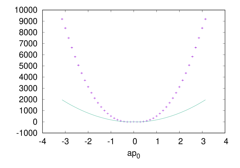
(a) Real part

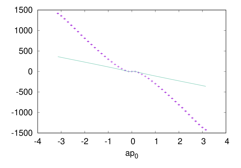
(b) Imaginary part

Figure 1: $\langle T(p)T(-p)\rangle$ for $D_{3}$, $L=44$, and $p_{1}=\pi/22$. The fitting curve (3.1) is depicted at once.

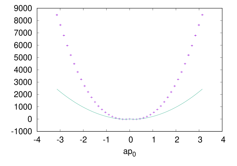
(a) Real part

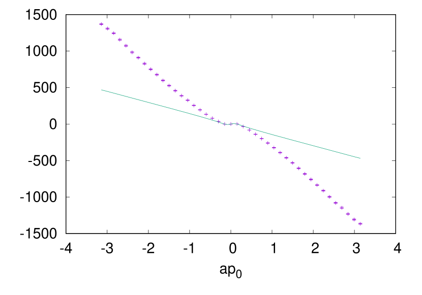
(b) Imaginary part

Figure 2: $\langle T(p)T(-p)\rangle$ for $D_{4}$, $L=42$, and $p_{1}=\pi/21$. The fitting curve (3.1) is depicted at once.

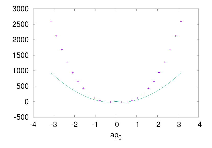
(a) Real part

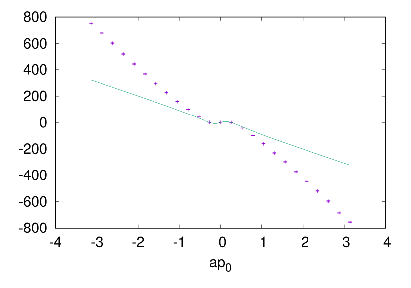
(b) Imaginary part

Figure 3: $\langle T(p)T(-p)\rangle$ for $E_{7}$, $L=24$, and $p_{1}=\pi/12$. The fitting curve (3.1) is depicted at once.

Table 7: The central charge obtained from the fit of the EMT correlator. The fitted momentum range is $\frac{2\pi}{L}\leq|p|<\frac{4\pi}{L}$.

Algebra	$L$	$\chi^{2}/\text{d.o.f.}$	$c$	Expected value
$D_{3}$	$8$	6.056	2.786(34)	1.5
	$16$	5.496	2.141(31)
	$24$	3.122	1.867(28)
	$32$	2.682	1.711(29)
	$40$	0.476	1.591(32)
	$44$	3.598	1.595(31)
$D_{4}$	$8$	3.216	2.907(36)	2
	$16$	3.738	2.509(34)
	$24$	1.946	2.466(42)
	$32$	2.832	2.202(40)
	$36$	1.109	2.211(70)
	$40$	2.276	2.175(48)
	$42$	1.177	2.172(48)
$E_{7}$	$8$	2.220	2.964(36)	2.666…
	$16$	1.800	2.639(35)
	$24$	1.364	2.638(47)

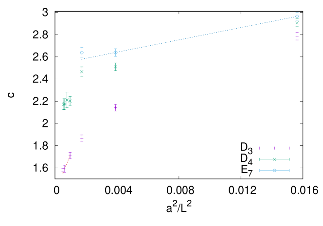
Figure 4: Systematic error estimation for the central charge.

As mentioned in Refs. Kamata:2011fr ; Morikawa:2018ops , it is interesting to plot the “effective central charge,” which is analogous to the Zamolodchikov’s $c$-function Zamolodchikov:1986gt ; Cappelli:1989yu . This is obtained from the fit in a variety of momentum regions from IR to UV; we take the fitted momentum regions as $\frac{2\pi}{L}n\leq|p|<\frac{2\pi}{L}(n+1)$ for $n\in\mathbb{Z}_{+}$. Then Fig. 5 shows that the “effective central charge” connects the IR central charge to an UV value $c\approx 6$. This number is consistent with the central charge $c=3N_{\Phi}$ in the expected free $\mathcal{N}=2$ SCFT. Recall that $N_{\Phi}$ is the number of supermultiplets in the free $\mathcal{N}=2$ WZ model, and we have set $N_{\Phi}=2$ in this paper.

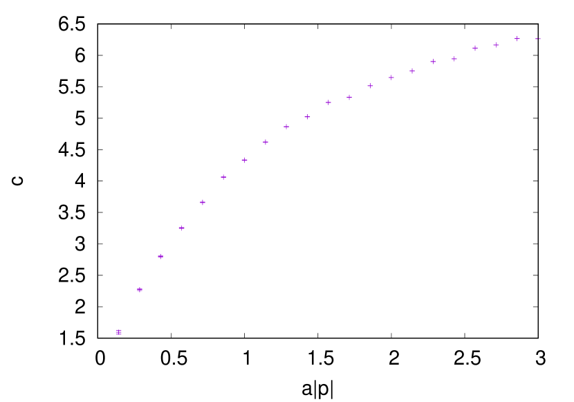
(a) For $D_{3}$ and $L=44$.

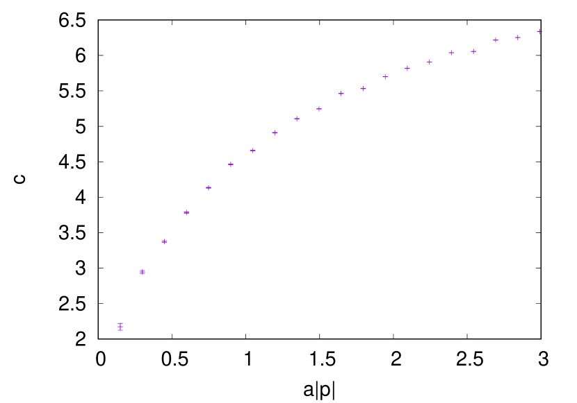
(b) For $D_{4}$ and $L=42$.

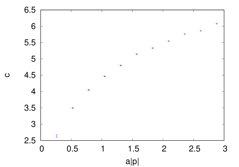
(c) For $E_{7}$ and $L=24$.

Figure 5: “Effective central charge,” which changes as the function of $|p|=\frac{2\pi}{L}n$ with fitted momentum regions, $\frac{2\pi}{L}n\leq|p|<\frac{2\pi}{L}(n+1)$, for $n\in\mathbb{Z}_{+}$.

6 Conclusion

In this paper, we numerically studied the two-dimensional $\mathcal{N}=2$ WZ model corresponding to the $D_{3}$, $D_{4}$, and $E_{7}$ minimal models. Utilizing the supersymmetry-preserving formulation with a momentum cutoff Kadoh:2009sp , we numerically determined the central charge from the IR behavior of the WZ model. Although the theoretical background of our computational approach is not clear so far, our results for the theories with two superfields are consistent with the conjectured correspondence between the LG model and the minimal series of SCFT. In the paper and the preceding studies Kawai:2010yj ; Kamata:2011fr ; Morikawa:2018ops , we have the numerical evidences of typical minimal models: the $A_{2}$, $A_{3}$, $D_{3}$, $D_{4}$, $E_{6}$, and $E_{7}$ models in Table 1; the $A_{4}$ or $E_{8}$ ($\cong A_{2}\otimes A_{4}$) minimal model is left to be simulated.

To investigate superstring theory by using our numerical approach, we may start from the numerical simulation of the $A_{4}$ minimal model, or simpler theories with several supermultiplets which is not a Gepner model.

References

- (1) J. Wess and B. Zumino, Nucl. Phys. B 70 (1974) 39. doi:10.1016/0550-3213(74)90355-1
- (2) P. Di Vecchia, J. L. Petersen and H. B. Zheng, Phys. Lett. 162B (1985) 327. doi:10.1016/0370-2693(85)90932-3
- (3) P. Di Vecchia, J. L. Petersen and M. Yu, Phys. Lett. B 172 (1986) 211. doi:10.1016/0370-2693(86)90837-3
- (4) P. Di Vecchia, J. L. Petersen, M. Yu and H. B. Zheng, Phys. Lett. B 174 (1986) 280. doi:10.1016/0370-2693(86)91099-3
- (5) W. Boucher, D. Friedan and A. Kent, Phys. Lett. B 172 (1986) 316. doi:10.1016/0370-2693(86)90260-1
- (6) D. Gepner, Nucl. Phys. B 287 (1987) 111. doi:10.1016/0550-3213(87)90098-8
- (7) A. Cappelli, C. Itzykson and J. B. Zuber, Nucl. Phys. B 280 (1987) 445. doi:10.1016/0550-3213(87)90155-6
- (8) A. Cappelli, Phys. Lett. B 185 (1987) 82. doi:10.1016/0370-2693(87)91532-2
- (9) D. Gepner and Z. a. Qiu, Nucl. Phys. B 285 (1987) 423. doi:10.1016/0550-3213(87)90348-8
- (10) D. Gepner, Nucl. Phys. B 296 (1988) 757. doi:10.1016/0550-3213(88)90397-5
- (11) A. Cappelli, C. Itzykson and J. B. Zuber, Commun. Math. Phys. 113 (1987) 1. doi:10.1007/BF01221394
- (12) A. Kato, Mod. Phys. Lett. A 2 (1987) 585. doi:10.1142/S0217732387000732
- (13) D. Gepner, Phys. Lett. B 199 (1987) 380. doi:10.1016/0370-2693(87)90938-5
- (14) D. A. Kastor, E. J. Martinec and S. H. Shenker, Nucl. Phys. B 316 (1989) 590. doi:10.1016/0550-3213(89)90060-6
- (15) C. Vafa and N. P. Warner, Phys. Lett. B 218 (1989) 51. doi:10.1016/0370-2693(89)90473-5
- (16) E. J. Martinec, Phys. Lett. B 217 (1989) 431. doi:10.1016/0370-2693(89)90074-9
- (17) W. Lerche, C. Vafa and N. P. Warner, Nucl. Phys. B 324 (1989) 427. doi:10.1016/0550-3213(89)90474-4
- (18) P. S. Howe and P. C. West, Phys. Lett. B 223 (1989) 377. doi:10.1016/0370-2693(89)91619-5
- (19) S. Cecotti, L. Girardello and A. Pasquinucci, Nucl. Phys. B 328 (1989) 701. doi:10.1016/0550-3213(89)90226-5
- (20) P. S. Howe and P. C. West, Phys. Lett. B 227 (1989) 397. doi:10.1016/0370-2693(89)90950-7
- (21) S. Cecotti, L. Girardello and A. Pasquinucci, Int. J. Mod. Phys. A 6 (1991) 2427. doi:10.1142/S0217751X91001192
- (22) S. Cecotti, Int. J. Mod. Phys. A 6 (1991) 1749. doi:10.1142/S0217751X91000939
- (23) E. Witten, Int. J. Mod. Phys. A 9 (1994) 4783 doi:10.1142/S0217751X9400193X [hep-th/9304026].
- (24) H. Kawai and Y. Kikukawa, Phys. Rev. D 83 (2011) 074502 doi:10.1103/PhysRevD.83.074502 [arXiv:1005.4671 [hep-lat]].
- (25) S. Kamata and H. Suzuki, Nucl. Phys. B 854 (2012) 552 doi:10.1016/j.nuclphysb.2011.09.007 [arXiv:1107.1367 [hep-lat]].
- (26) O. Morikawa and H. Suzuki, PTEP 2018 (2018) no.8, 083B05 doi:10.1093/ptep/pty088 [arXiv:1805.10735 [hep-lat]].
- (27) Y. Kikukawa and Y. Nakayama, Phys. Rev. D 66 (2002) 094508 doi:10.1103/PhysRevD.66.094508 [hep-lat/0207013].
- (28) D. Kadoh and H. Suzuki, Phys. Lett. B 684 (2010) 167 doi:10.1016/j.physletb.2010.01.022 [arXiv:0909.3686 [hep-th]].
- (29) H. Nicolai, Phys. Lett. 89B (1980) 341. doi:10.1016/0370-2693(80)90138-0
- (30) H. Nicolai, Nucl. Phys. B 176 (1980) 419. doi:10.1016/0550-3213(80)90460-5
- (31) G. Parisi and N. Sourlas, Nucl. Phys. B 206 (1982) 321. doi:10.1016/0550-3213(82)90538-7
- (32) S. Cecotti and L. Girardello, Annals Phys. 145 (1983) 81. doi:10.1016/0003-4916(83)90172-0
- (33) S. Nicolis, Phys. Part. Nucl. 49 (2018) 899 doi:10.1134/S1063779618050313 [arXiv:1712.07045 [hep-th]].
- (34) A. B. Zamolodchikov, JETP Lett. 43 (1986) 730 [Pisma Zh. Eksp. Teor. Fiz. 43 (1986) 565].
- (35) A. Cappelli and J. I. Latorre, Nucl. Phys. B 340 (1990) 659. doi:10.1016/0550-3213(90)90463-N
- (36) S. Cecotti, Nucl. Phys. B 355 (1991) 755. doi:10.1016/0550-3213(91)90493-H
- (37) B. R. Greene, C. Vafa and N. P. Warner, Nucl. Phys. B 324 (1989) 371. doi:10.1016/0550-3213(89)90471-9
- (38) E. Witten, Nucl. Phys. B 403 (1993) 159 [AMS/IP Stud. Adv. Math. 1 (1996) 143] doi:10.1016/0550-3213(93)90033-L [hep-th/9301042].
- (39) J. Bartels and J. B. Bronzan, Phys. Rev. D 28 (1983) 818. doi:10.1103/PhysRevD.28.818
- (40) S. D. Drell, M. Weinstein and S. Yankielowicz, Phys. Rev. D 14 (1976) 487. doi:10.1103/PhysRevD.14.487
- (41) S. D. Drell, M. Weinstein and S. Yankielowicz, Phys. Rev. D 14 (1976) 1627. doi:10.1103/PhysRevD.14.1627
- (42) P. H. Dondi and H. Nicolai, Nuovo Cim. A 41 (1977) 1. doi:10.1007/BF02730448
- (43) L. H. Karsten and J. Smit, Phys. Lett. 85B (1979) 100. doi:10.1016/0370-2693(79)90786-X
- (44) M. Kato, M. Sakamoto and H. So, JHEP 0805 (2008) 057 doi:10.1088/1126-6708/2008/05/057 [arXiv:0803.3121 [hep-lat]].
- (45) G. Bergner, JHEP 1001 (2010) 024 doi:10.1007/JHEP01(2010)024 [arXiv:0909.4791 [hep-lat]].
- (46) E. Witten, Nucl. Phys. B 202 (1982) 253. doi:10.1016/0550-3213(82)90071-2
- (47) S. Cecotti and L. Girardello, Phys. Lett. 110B (1982) 39. doi:10.1016/0370-2693(82)90947-9
- (48) S. Catterall and S. Karamov, Phys. Rev. D 65 (2002) 094501 doi:10.1103/PhysRevD.65.094501 [hep-lat/0108024].
- (49) J. Polchinski, “String theory. Vol. 1: An introduction to the bosonic string,” Cambridge University Press, 1998, 402 p.
- (50) J. Polchinski, “String theory. Vol. 2: Superstring theory and beyond,” Cambridge University Press, 1998, 531 p.
- (51) A. A. Tseytlin, Phys. Lett. B 194 (1987) 63. doi:10.1016/0370-2693(87)90770-2
- (52) J. Polchinski, Nucl. Phys. B 303 (1988) 226. doi:10.1016/0550-3213(88)90179-4