Bogomol’nyi Equations for Vortices in Born–Infeld–Higgs Systems

Abstract

We study vortex solutions in the Born–Infeld theory coupled with a complex scalar field. We show that for a specific form of the “Higgs” potential the vortex satisfies a set of Bogomol’nyi-type equations. Another model, with nonlinear interaction between gauge and Higgs fields, is also considered. We show how it is derived from a supersymmetric extension of the Born–Infeld theory with a minimally coupled complex scalar field.

1 Introduction

The idea that cosmic strings [1] might provide the seeds for galaxy formation [2] has attracted the attention of particle physicists as well as astrophysicists in recent years [3]. The scenario of cosmic-string theory seems very simple and highly predictive. Cosmic strings also have direct consequences which can be checked by astronomical observations [4].

We find that, in many research papers, cosmic strings are represented by Nielsen–Olesen vortices [5] in Abelian Higgs systems. In the model of this type, the $U(1)$ gauge field is not the ordinary electromagnetic one, but considered as a field associated with a spontaneously broken part in a grand unified model.

In unification schemes at very high energy such as SUGRA-GUTs [6] and superstring(-inspired) models [7], corrections to the field equations exist in general. They have a mass scale of order of the Planck mass; above the Planck energy, nonrenormalizable interactions become important. The effects of such nonrenormalizable correction terms have been studied in diverse contexts, especially through the investigation of physics in very early universe.

We can derive effective actions from string theories by various methods [9]. From open-string theory [10], we can get the Born–Infeld action [11] for gauge fields. Although the open-string theory was considered as phenomenologically unfavorable, four-dimensional ones have been investigated by several authors very recently [12].

If the nonlinear gauge action is utilized in a grand unification scheme, a topological defect, which can possibly be produced in a phase transition, might have different structure than in the usual model. Conversely, we can suppose that topological defects and their consequences in the very early universe might give some clues to physics on very-high-energy scale.

We must notice that the shape of Higgs potential could be changed and nonrenormalizable in the unified models with spontaneously broken symmetry. If we take the possibility into account, we have a great variety of models, in which vortexlike solutions exit. In this paper, we restrict ourselves to considering an interesting class of gauge Higgs models.

We would like to seek gauge Higgs models, in which the vortex-type solution can be described as a solution to a set of first-order differential equations. Such equations are known as self-dual or Bogomol’nyi equations [13] in gauge field theories which possess topological solutions, such as vortices and monopoles. Bogomol’nyi-type equations hold only if couplings in a model take specific values. In general, if the self-dual equations are satisfied, the mass (or the energy density) of the topological object is determined analytically, and it often gives a bound for the mass of the object in a more generic class of models. Furthermore, a solution which represents multicentered topological objects can be obtained from the analysis of Bogomol’nyi-type equations[14].

We choose Born–Infeld action as a gauge-field action, since it has been motivated by string theories recently [11] and is a unique action which describes causal propagation of photons, in spite of its nonlinearity [15]. We assume a kinetic term of a complex Higgs scalar field as a minimal one, i.e., a quadratic in covariant derivatives. Thus the choice of models is attributed to determination of the form of the Higgs potential. The present work was partly prompted by a recent paper by Jackiw and Weinberg [16], in which they obtain a self-dual relation in a Chern–Simons Higgs system in three-dimensional space–time.

In Sec. 2, we determine the potential and show the vortex solutions associated with it. In Sec. 3, we examine another possibility of existence of nonminimal coupling between gauge and Higgs fields. A model is shown to possess Bogomol’nyi equations which are the same as those of the usual Abelian Higgs model. The relation to supersymmetry is studied. Section 4 is devoted to the conclusion.

2 Bogomol’nyi Equations, Potentials and Vortices

We start from a coupled system of a complex scalar field and $U(1)$ gauge field which is governed by nonlinear Born–Infeld action [11] in two (spatial) dimensions. The total action is

$$S=\int d^{2}\hat{x}\left[\frac{\hat{\beta}^{2}}{e^{2}}\left\{\sqrt{\det\left(\delta_{ij}+\frac{1}{\hat{\beta}}\hat{F}_{ij}\right)}-1\right\}+(\hat{D}_{i}\hat{\phi})(\hat{D}^{i}\hat{\phi})^{*}+\hat{V}(|\hat{\phi}|)\right]\,,$$ (1)

where $\hat{\phi}$ complex scalar field, $\hat{A}_{i}$ is a $U(1)$ gauge field, and $\hat{F}_{ij}=\partial_{i}\hat{A}_{j}-\partial_{j}\hat{A}_{i}$ ($i,j=1,2$) is the field strength. The covariant derivative is defined as $\hat{D}_{i}=\partial_{i}+i\hat{A}_{i}$.

We require that the Higgs potential $\hat{V}(|\hat{\phi}|)$ have a minimum at $|\hat{\phi}|=v$. Further, we assume normalization so that $\hat{V}(v)=0$.

Rescaling the dimensions of the fields and length by using $v$ according to

$$\hat{\phi} = v\phi\,,$$ (2)

$$\hat{A}_{i} = evA_{i}\,,$$ (3)

$$\hat{x}^{i} = (ev)^{-1}x^{i}$$ (4)

leads to

$$S=v^{2}\int d^{2}{x}\left[{\beta}^{2}\left\{\sqrt{\det\left(\delta_{ij}+\frac{1}{{\beta}}{F}_{ij}\right)}-1\right\}+({D}_{i}{\phi})({D}^{i}{\phi})^{*}+{V}(|{\phi}|)\right]\,,$$ (5)

where $\beta=\hat{\beta}/(e^{2}v^{2})$. The rescaled potential $V(|\phi|)=(e^{2}v^{4})^{-1}\hat{V}(|\hat{\phi}|)$ has a minimum at $|\phi|=1$.

When the $U(1)$ symmetry is broken in the above system, we expect the existence of classical vortex solutions with finite energy (in two dimensions). In the case of the usual Maxwell action, a critical relation between the gauge coupling constant and the Higgs self-coupling leads to the vortex solution’s obeying Bogomol’nyi-type equations [13, 17]. In this section, we show that the vortex in the Born–Infeld Higgs system satisfies Bogomol’nyi-type equations for a specific choice or the Higgs potential.

Here we take the simplest Ansätze:

$$\phi=f(r)e^{in\theta}\,,\qquad A_{i}=-\varepsilon_{ij}\frac{x^{j}}{r^{2}}n[P(r)-1]\,,$$ (6)

where $r$ is the radial distance form the origin (i.e., the center of the vortex), $\theta$ is the azimuthal angle, $\varepsilon_{ij}$ is the Levi-Civita tensor, and $n$ corresponds to the winding number of the configuration. We consider $n$ as a positive integer throughout this paper, since the case with negative winding number can be immediately constructed from the positive-$n$ case. If the energy of the vortex is to be finite, $|\phi|=f$ must tend to one and $D_{i}\phi$ must vanish at spatial infinity. Of course, the fields must not be singular also at the origin. Therefore the boundary conditions for a vortex solution are

$$P(0)=1\,,\qquad f(0)=0\,,$$ (7)

$$P(\infty)=0\,,\qquad f(\infty)=1\,.$$ (8)

Hereafter we study the field equations in terms of these cylindrical Ansätze and boundary condition.

The field equations for the scalar and gauge fields become

$$\frac{(rf)^{\prime}}{r}=\frac{n^{2}P^{2}f}{r^{2}}+\frac{1}{2}\frac{\partial V(f)}{\partial f}\,,$$ (9)

$$\left[\left\{1+\left(\frac{nP^{\prime}}{\beta r}\right)^{2}\right\}^{-1/2}\frac{P^{\prime}}{r}\right]^{\prime}=\frac{2f^{2}P}{r}\,,$$ (10)

when the prime denotes the derivative with respect to $r$.

Our purpose is to find differential equations of first order whose solutions automatically satisfy the above field equations, and to find a suitable form of the symmetry breaking potential. We begin with the relation concerned with the covariant derivative on the scalar field.

Since we assume that the kinetic term of the complex scalar is the same as that of the usual Abelian Higgs model, we may anticipate that one of the first order self-dual equations is

$$D_{1}\phi+iD_{2}\phi=0\,,$$ (11)

just as in the case of vortices in Abelian Higgs model [14]. Substitution of the Ansätze into Eq. (11) gives

$$f^{\prime}=\frac{nPf}{r}\,.$$ (12)

Using this equation twice in the field equation (9), we can obtain a first-order differential equation,

$$\frac{nP^{\prime}}{r}=\frac{1}{2f}\frac{\partial V(f)}{\partial f}\,.$$ (13)

We determine the potential by demanding that the first order equations (13) and (12) satisfy another field equation, (10). Performing integration after substituting the first two equations into the third, we obtain

$$\frac{1}{2f}\frac{\partial V(f)}{\partial f}=\frac{f^{2}-1}{\sqrt{1-\frac{(f^{2}-1)^{2}}{\beta^{2}}}}\,,$$ (14)

since we require that the vanishing minimum of the potential be located at $f=1$. Once more, integration leads to the result, i.e.

$$V(f)=\beta\left\{1-\sqrt{1-\frac{(f^{2}-1)^{2}}{\beta^{2}}}\right\}\,,$$ (15)

where the minimum value of the potential is normalized to be zero. The schematic view of the potential is displayed in Fig. 1. Evidently, we can replace $f$ by $|\phi|$ to get the potential of complex scalar field. It is obvious that this potential reduces to the usual $\phi^{4}$-type potential in the limit of $\beta\rightarrow\infty$.

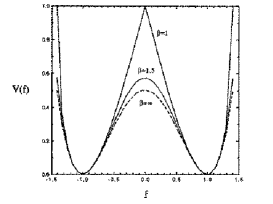
Figure 1: Schematic view of the potential $V(\phi)$. The solid, dotted and dashed lines correspond to $\beta=1,1.5$, and $\infty$, respectively.

The potential cannot be defined in the region

$$(|\phi|^{2}-1)^{2}\geq\beta^{2}\,.$$ (16)

For our present purpose to obtain vortex solutions, it is sufficient that the potential is defined as the form of Eq. (15) in the range $0\leq f\leq 1+\epsilon$, where $\epsilon$ is an arbitrary small quantity. Hence, we restrict $\beta$ to be greater than one, and $V(\phi)$ can be regarded as an arbitrary function of $|\phi|$ for $|\phi|>1$.

It can be shown that the Higgs- and the gauge-field masses are equal, i.e.

$$m_{H}^{2} = \frac{1}{2}\left|\frac{\partial~{}2V}{\partial f^{2}}\right|_{f=1}\cdot(ev)^{2}=2e^{2}v^{2}\,,$$ (17)

$$m_{A}^{2} = \left|2f^{2}\right|_{f=1}\cdot(ev)^{2}=2e^{2}v^{2}\,.$$ (18)

Now we look into the behavior of vortex solutions. At large $r$, Eq. (12) and (13) with (14) can be approximated by linear equations in terms of $P$ and $\delta\equiv 1-f$. The linearized equations are the same as those of the Abelian Higgs model and are therefore independent of $\beta$. The behavior of solution at infinity is

$$f \simeq 1-CK_{0}(\sqrt{2}r)\,,$$ (19)

$$P \simeq C\frac{\sqrt{2}r}{n}K_{1}(\sqrt{2}r)\,,$$ (20)

where $K_{0}$ and $K_{1}$ are the modified Bessel functions.

By performing a power-series expansion, we obtain the behavior at small $r$. To the leading order, the solution is (when $\beta\neq 1$)

$$f = \frac{A(\sqrt{2}r)^{n+2}}{4(n+2)\sqrt{1-\frac{1}{\beta^{2}}}}+O[(\sqrt{2}r)^{n+4}]\,,$$ (21)

$$P = 1-\frac{(\sqrt{2}r)^{2}}{4n\sqrt{1-\frac{1}{\beta^{2}}}}+O[(\sqrt{2}r)^{4}]\,.$$ (22)

The constants $C$ [in (19) and (20)] and $A$ [in (21) and (22)] are not determined by the expansions in their proper regions. The detailed behavior of vortex configurations is obtained by numerical calculation of the set of Bogomol’nyi-type equations. We use the computational code COLSYS [18]. The results of the numerical solution for the equations are shown in Figs. 2, 3 and 4, for $\beta=\infty,1.5$ and $1$ respectively.

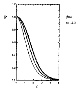
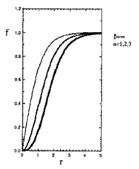
(a)                                           (b)

Figure 2: The functions $P(r)$ [in (a)] and $f(r)$ [in (b)] in the case of $\beta=\infty$. The lines correspond to the winding numbers $n=3,2$ and $1$, in order of thickness.

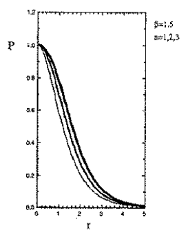
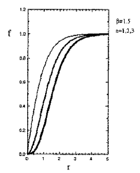
(a)                                           (b)

Figure 3: The functions $P(r)$ [in (a)] and $f(r)$ [in (b)] in the case of $\beta=1.5$. The lines correspond to the winding numbers $n=3,2$ and $1$, in order of thickness.

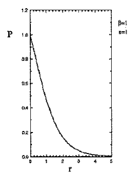
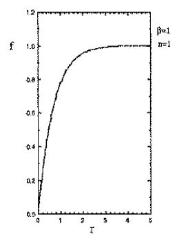
(a)                                           (b)

Figure 4: The functions $P(r)$ [in (a)] and $f(r)$ [in (b)] in the case of $\beta=1$. The lines correspond to the winding number $n=1$.

The limiting case with $\beta=1$ attracts much interest. As we have seen, the behavior of the solutions very distant from the core of the vortex is independent of $\beta$. Hence we pay attention to examination of the behavior in the vicinity of the origin. Absence of the singularity in the vector field at the origin requires $P(0)=1$. Thus $f$ behaves like $r^{n}$ near the origin. The $P-1$ must behave like $r^{2-n}$, according to Eq. (12)–(14). $P$ can converge to $1$ if and only if $n=1$, and then we have a finite magnetic flux. Unlike the case of general values of $\beta$, the merger of two-vortices into a vortex with $n=2$ is impossible. The results of the numerical solutions of the equations are shown in Fig. 4 for $\beta=1$ and $n=1$.

The energy of the vortex is obtained by the substitution of the solution into the integration:

$$E=v^{2}\int d^{2}x\left[\beta^{2}\left\{\sqrt{1+\frac{n^{2}{P^{\prime}}^{2}}{\beta^{2}r^{2}}}-\sqrt{1-\frac{(f^{2}-1)^{2}}{\beta^{2}}}\right\}+{f^{\prime}}^{2}+\frac{n^{2}P^{2}f^{2}}{r^{2}}\right]\,.$$ (23)

We rearrange the expression (23) to give

$$E=v^{2}\int d^{2}x\left[\left(f^{\prime}-\frac{nPf}{r}\right)^{2}+\frac{1}{2}\frac{1}{\sqrt{1+\left(\frac{n{P^{\prime}}}{\beta r}\right)^{2}}}\left\{\frac{nP^{\prime}}{r}-\sqrt{1+\left(\frac{n{P^{\prime}}}{\beta r}\right)^{2}}(f^{2}-1)\right\}^{2}\right.$$

$$+\left.\frac{1}{2}\frac{\beta^{2}}{\sqrt{1+\left(\frac{n{P^{\prime}}}{\beta r}\right)^{2}}}\left\{\sqrt{1+\left(\frac{n{P^{\prime}}}{\beta r}\right)^{2}}\sqrt{1-\frac{(f^{2}-1)^{2}}{\beta^{2}}}-1\right\}^{2}+\frac{1}{r}\{nP(f^{2}-1)\}^{\prime}\right]\,,$$ (24)

with

$$E\geq 2\pi nv^{2}\,.$$ (25)

The bound is attained if the self-dual equations, (12) and (13), are satisfied.

If the vortex is embedded in three-dimensional space, it represents an infinite, straight cosmic string. In this case, the tension of the string is given by $E$ obtained above. Of course, $E$ is also the energy density per unit length of the cosmic sting. Moreover, we find that, owing to the Bogomol’nyi-type equations, all the other components of the stress tensor, i.e. pressures in the direction perpendicular to the string, vanish.

3 Nonlinear Coupling between Gauge and Higgs Field and Supersymmetry

In this section, we construct another model in which self-dual vortices exist. In the present analysis, we permit nonminimal coupling between gauge and Higgs fields while the kinetic term of the complex scalar is still assumed to be the canonical one. To be more concrete, we assume a multiplicative form of modified Born–Infeld action,

$$S=\int d^{2}\hat{x}\left[\frac{\hat{\beta}^{2}}{e^{2}}\left\{\hat{G}(|\hat{\phi}|)\sqrt{-\det\left(\eta_{mn}+\frac{1}{\hat{\beta}}\hat{F}_{mn}\right)}-1\right\}+(\hat{D}_{m}\hat{\phi})(\hat{D}^{m}\hat{\phi})^{*}\right]\,,$$ (26)

where $\hat{G}(|\hat{\phi}|)$ is a function of the Higgs scalar field $\hat{\phi}$ and $m,n$ are the suffixes of $d$-dimensional space–time.

Here we require that $\hat{G}(|\hat{\phi}|)$ have an extremum at $|\hat{\phi}|=v$, and after symmetry breaking the action (26) becomes the standard Born–Infeld action.

The analysis of the condition on $\hat{G}$ for existence of self-dual equations can be performed in a way similar to that in Sec. 2. We show only the result here. The self-dual equations can be established if we choose $\hat{G}(|\hat{\phi}|)$ as

$$\hat{G}(|\hat{\phi}|)=\sqrt{1+\frac{e^{4}(|\hat{\phi}|^{2}-v^{2})^{2}}{\hat{\beta}^{2}}}\,.$$ (27)

Note that in the limit $\beta\rightarrow\infty$, the action reduces to the usual Abelian Higgs model. The Higgs- and gauge-field masses are the same as those in the model of Sec. 2.

When we rescale the fields and length as in Sec. 2, and use the same Ansätze, (6) for a vortex, Bogomol’nyi-type equations are expressed as

$$f^{\prime} = \frac{nPf}{r}\,,$$ (28)

$$\frac{nP^{\prime}}{r} = f^{2}-1\,.$$ (29)

These equations are perfectly coincident with those of the usual Abelian Higgs model with critical relation between couplings.

The energy in two-dimensional subsystem can be written as

$$E=v^{2}\int d^{2}x\left[\beta^{2}\left\{\sqrt{1+\frac{(f^{2}-1)^{2}}{\beta^{2}}}\sqrt{1+\frac{n^{2}{P^{\prime}}^{2}}{\beta^{2}r^{2}}}-1\right\}+{f^{\prime}}^{2}+\frac{n^{2}P^{2}f^{2}}{r^{2}}\right]$$

$$=v^{2}\int d^{2}x\left[\left(f^{\prime}-\frac{nPf}{r}\right)^{2}+\frac{1}{2}\frac{\sqrt{1+\frac{(f^{2}-1)^{2}}{\beta^{2}}}}{\sqrt{1+\left(\frac{n{P^{\prime}}}{\beta r}\right)^{2}}}\left\{\frac{nP^{\prime}}{r}-\frac{\sqrt{1+\left(\frac{n{P^{\prime}}}{\beta r}\right)^{2}}}{\sqrt{1+\frac{(f^{2}-1)^{2}}{\beta^{2}}}}(f^{2}-1)\right\}^{2}\right.$$

$$+\left.\frac{1}{2}\beta^{2}\frac{\sqrt{1+\frac{(f^{2}-1)^{2}}{\beta^{2}}}}{\sqrt{1+\left(\frac{n{P^{\prime}}}{\beta r}\right)^{2}}}\left\{\frac{\sqrt{1+\left(\frac{n{P^{\prime}}}{\beta r}\right)^{2}}}{\sqrt{1+\frac{(f^{2}-1)^{2}}{\beta^{2}}}}-1\right\}^{2}+\frac{1}{r}\{nP(f^{2}-1)\}^{\prime}\right]\,.$$ (30)

which is the same as that of the model in Sec. 2; and this is an identical relation to the bound in the usual Abelian Higgs model.

Note that, in the present model, even energy-density distribution of the vortex solution is independent of $\beta$. The pressure in the direction perpendicular to the straight string vanishes as in the previous model.

From now on, we will show how the special form of the action of the present model arises very naturally from a supersymmetric generalization of Born–Infeld theory. We discuss here an indirect evidence for connection between our model and supersymmetry. We will show the complete argument in future publications.

We start with construction of $d=4$, $N=1$ supersymmetric generalization of the Born–Infeld theory. A general discussion can be found in Ref. [19], on the case without matter couplings. In the present investigation, we consider a coupling to a complex scalar field, but we begin with a simplified action. If only magnetic fields are present in two-dimensional subsystem, say, the $x$-$y$ plane, then the Born–Infeld Higgs action is equivalent to

$$\int d^{4}\hat{x}\left[\frac{\hat{\beta}^{2}}{e^{2}}\left\{\sqrt{1+\frac{1}{2\hat{\beta}^{2}}\hat{F}_{mn}\hat{F}^{mn}}-1\right\}+(\hat{D}_{m}\hat{\phi})(\hat{D}^{m}\hat{\phi})^{*}\right]\,,$$ (31)

where $m$ and $n$ run over $0,1,2,3$. In present four-dimensional case, this replacement of action is equivalent to omitting $(F^{*}F)^{2}$ term [19], which has no effect on dynamics of the two-dimensional subsystem.

Let us consider a supersymmetric generalization of the action (31) and its coupling to a complex scalar field with symmetry breaking. To this end, it is most convenient to use the superfield formalism. The curvature supermultiplet $W_{\alpha}$, whose components are $A_{m},\psi,D$ ($\psi$ is a photino field and $D$ an auxiliary one), is given by

$$W_{\alpha}=-\frac{1}{4}\bar{D}^{\beta}\bar{D}_{\beta}D_{\alpha}V\,,$$ (32)

where $V$ is a vector multiplet. We can also construct $W_{\alpha\beta}\equiv D_{\alpha}W_{\beta}$, though $\bar{D}_{\alpha}W_{\beta}=0$. For the expression for the covariant derivative, see Ref. [20]. The multiplet $W^{\alpha}D_{\alpha}V+\bar{W}^{\alpha}\bar{D}_{\alpha}V$, built from the superfields, contains the term $2D^{2}-F^{2}$ in its last ($D$) component. Here $D$ is an auxiliary field. On the other hand, we find that the superfield $W\alpha W_{\alpha}+\bar{W}^{\alpha}\bar{W}_{\alpha}$ has the combination $2D^{2}-F^{2}$ as the first component. Therefore we can construct any supersymmetric gauge model whose action is an arbitrary function of $F^{2}$, by expanding the function in a form of power series and using these superfields.

To introduce a complex scalar field, we use two chiral scalar multiplets, $\Phi$ and $\Phi^{+}$. The scalar kinetic term is involved in the combination $\Phi^{+}e^{2V}\phi$ as its last component. (Note that the gauge coupling is absorbed in the fields in our notation.) It also includes the coupling between the auxiliary field $D$ and the scalar field.

Further we introduce a Fayet–Illiopoulos term [21] to break the $U(1)$ symmetry. This term is linear in the superfield $V$.

Putting the above terms together, we obtain a supersymmetric generalization of the Born–Infeld theory with symmetry breaking. If we set the fermion fields to zero, the action for the bosonic fields is:

$$S\approx\int d^{4}{x}\left[{\beta}^{2}\left\{\sqrt{1+\frac{1}{{\beta}^{2}}\left(\frac{1}{2}F^{2}-D^{2}\right)}-1\right\}+({D}_{m}{\phi})({D}^{m}{\phi})^{*}+(|\phi|^{2}-1)D\right]\,,$$ (33)

where the dimensionful quantities have been properly scaled again.

Note here that the gauge action is obtained by the replacement ${}^{2}\rightarrow F^{2}-2D^{2}$ in the Born–Infeld action. Eliminating the auxiliary field $D$ by using its field equation, we get

$$S\approx\int d^{4}{x}\left[{\beta}^{2}\left\{\sqrt{1+\frac{(|\phi|^{2}-1)^{2}}{{\beta}^{2}}}\sqrt{1+\frac{1}{{\beta}^{2}}\frac{1}{2}F^{2}}-1\right\}+({D}_{m}{\phi})({D}^{m}{\phi})^{*}\right]\,.$$ (34)

This action is precisely equal to (26) with (27) up to normalization.

The intimate connection between self-duality and supersymmetry has been studied in various models [22]. The both are related to the existence of fermionic zero modes. We must clarify the coupling of fermion fields to the action and the full supersymmetric extension of the Born–Infeld theory which contains general higher-order terms, such as $(F^{*}F)^{2}$ [27].

4 Conclusion

In this paper, we have studied the nonlinear gauge Higgs models whose vortex solutions are governed by a set of first-order equations.

In the model shown in Sec. 2, the vortex solutions are slightly modified in their shape for finite $\beta$. For smaller $\beta$, the “string” reduces its thickness, while its energy per unit length is still unchanged. If we apply the model to bosonic superconducting strings [23], the allowed parameter region for existence of the solution will be enlarged because of the higher energy density of the false vacuum. Although the calculation of magnitude of critical current or other characteristic quantities is necessary, no remarkable effect on properties of possible cosmic strings may be expected because of the restriction on the range of the coupling, $\beta>1$.

We did not consider the analysis of multivortex configuration. This is an interesting subject to study, especially in the case of $\beta\approx 1$.

A generalization to non-Abelian gauge models in very attractive [24]. Mechanisms of gauge symmetry breaking must be studied in the Born–Infeld-type theory. At the same time, we wish to study topological defects in the model, such as monopoles and strings. We are also interested in the interrelation between the gauge sector and the axionic sector in the string-inspired models. In particular, we hope to study the structure of comic strings in such models. Recently, the present authors and Nakamula have considered gauge-field cosmic strings with compactified space [25]. Applying such a method to our Born–Infeld Higgs system, we might clarify the existence of several types of cosmic strings and their implications for cosmology.

In this paper we adopted a minimal kinetic term for a complex scalar. It is not unnatural to consider noncanonical kinetic term like a nonlinear sigma model. This type of the kinetic term frequently appears in the literature of supergravity theory [6, 26]. The consideration of this possibility might allow variety of the form of the potential which leads to self-dual equations.

The nonlinear model treated of in Sec. 3 will be carefully examined further. Not only global but local supersymmetry must be considered, since we also wish to study the relation to unified, phenomenologically viable models.

References

- [1] A. Vilenkin, Phys. Rep. 121 (1985) 263.
- [2] Y. B. Zel’dovich, Mon. Not. R. Astron. Soc. 192 (1980) 663.
- [3] See, for example, Cosmic Strings: The Current Status—Proceedings of the Yale Workshop (1988), eds. F. S. Accetta and L. M. Krauss (World Scientific, Singapore, 1989).
- [4] A. Vilenkin, Astrophys. J. 282 (1984) L51; F. R. Bouchet, D. P. Bennett and A. Stebbins, Nature 335 (1988) 410; C. Hogan and M. Rees, Nature 311 (1984) 109.
- [5] N. B. Nielsen and P. Olesen, Nucl. Phys. B61 (1973) 45.
- [6] H. P. Nilles, Phys. Rep. 110 (1984) 1.
- [7] See for example, J. L. Hewett and T. G. Rizzo, Phys. Rep. 183 (1989) 193.
- [8] J. Ellis, K. Enqvist, D. Nanopoulos, K. Olive and M. Srednicki, Phys. Lett. B152 (1985) 175; R. Holman, P. Ramond and C. Ross, Pays. Lett. B137 (1984) 343; I. Antoniadis, J. Ellis, J. Hagelin and D. Nanopoulos, Phys. Lett. B205 (1983) 459; B208 (1983) 209.
- [9] C. G. Callan, E. J. Martinec, M. J. Perry and D. Friedan, Nucl. Phys. B262 (1985) 593; E. S. Fradkin and A. A. Tseytlin, Nucl. Phys. B261 (1986) 1; T. Banks, D. Nemechansky and A. Sen, Nucl. Phys. B277 (1986) 67. G. Curci and G. Paffuti, Nucl. Phys. B286 (1987) 399; M. J. Bowick and S. G. Rajeev, Nucl. Phys. B293 (1987) 348. D. Gross and E. Witten, Nucl. Phys. B277 (1986) 1.
- [10] A. A. Abouelsaoud, C. G. Callan, C. R. Nappi and S. A. Yost, Nucl. Phys. B280 (1987) 599.
- [11] M. Born and L. Infeld, Proc. R. Soc. London A144 (1934) 425.
- [12] Z. Bern and D. C. Dunbar, Phys. Rev. Lett 64 (1990) 827 and references there in.
- [13] E. B. Bogomol’nyi, Sov. J. Nucl. Phys. 24 (1976) 449.
- [14] C. H. Taubes, Commun. Math. Phys. 72 (1980) 277.
- [15] J. Plebanski, “Lectures on Nonlinear Electrodynamics” (1968), upublished. (cited in Ref. 19); T. Taniuti, Suppl. Prog. Theor. Phys. 9 (1959) 69.
- [16] R. Jackiw and E. Weinberg, Phys. Rev. Lett. 64 (1990) 2234.
- [17] H. J. de Vega and F. A. Schaposnik, Phys. Rev. D14 (1976) 1100; L. Jacobs and C. Rebbi, Phys. Rev. B19 (1979) 4486; E. Weinberg, Phys. Rev. D19 (1979) 3008.
- [18] U. Ascher, J. Christiansen and R. D. Russel, COLSYS: A Collocation Code for Boundary Value Problems—Proceedings of the Conference on CODES FOR BVP-S IN ODE-S (Houston, Texas, 1978).
- [19] S. Deser and R. Puzalowski, J. Phys. A13 (1980) 2501.
- [20] J. Wess and J. Bagger, Supersymmetry and Supergravity (Princeton University Press, New Jersey, 1983)
- [21] P. Fayet and S. Ferrara, Phys. Rep. 32 (1977) 249.
- [22] E. Witten and D. Olive, Phys. Lett. B78 (1978) 97.
- [23] E. Witten, Nucl. Phys. B249 (1985) 557.
- [24] P. C. Argyres and C. R. Nappi, Nucl. Phys. B330 (1990) 151 and references there in.
- [25] A. Nakamula, S. Hirenzaki and K. Shiraishi, Nucl. Phys. B339 (1990) 533.
- [26] A. Lahanas and D. V. Nanopoulos, Phys. Rep. 145 (1987) 1.
- [27] S. Cecotti and S. Ferrara, Phys. Lett. B187 (1987) 335.