Gravitational waves and electroweak baryogenesis in a global study of the extended scalar singlet model

Abstract

We perform a global fit of the extended scalar singlet model with a fermionic dark matter (DM) candidate. Using the most up-to-date results from the Planck measured DM relic density, direct detection limits from the XENON1T (2018) experiment, electroweak precision observables and Higgs searches at colliders, we constrain the 7-dimensional model parameter space. We also find regions in the model parameter space where a successful electroweak baryogenesis (EWBG) can be viable. This allows us to compute the gravitational wave (GW) signals arising from the phase transition, and discuss the potential discovery prospects of the model at current and future GW experiments. Our global fit places a strong upper and lower limit on the second scalar mass, the fermion DM mass and the scalar-fermion DM coupling. In agreement with previous studies, we find that our model can simultaneously yield a strong first-order phase transition and saturate the observed DM abundance. More importantly, the GW spectra of viable points can often be within reach of future GW experiments such as LISA, DECIGO and BBO.

1 Introduction

The discovery of the Higgs boson at the LHC Aad:2012tfa; Chatrchyan:2012xdj has finally completed the Standard Model (SM) of particle physics. Not only does it provide a new way to study the properties of the Higgs boson, it also offers a way to investigate the details of electroweak symmetry breaking (EWSB). Meanwhile, a more recent observation of the first gravitational wave (GW) signal Abbott:2016blz and subsequent discoveries Abbott:2016nmj; Abbott:2017ylp; Abbott:2017vtc; Abbott:2017oio; TheLIGOScientific:2017qsa; Monitor:2017mdv; Abbott:2017gyy have opened up a new window to probe the early history of our universe. In particular, rather violent events such as the first-order electroweak phase transition (EWPT) would necessarily leave GW imprints. With the current and future generations of ground/space-based GW experiments, we can hope to observe such signals Caprini:2015zlo; Weir:2017wfa; Caprini:2018mtu. The existence of dark matter (DM) also offers a way to probe the early history of our universe. With the current generation of direct DM searches, experiments are probing the DM-nucleon interaction with increasing sensitivity and placing strong limits on the allowed particle DM models.

Motivated by the above experimental probes that are constantly developing, we revisit an extended scalar singlet extension of the SM in this paper. In particular, we focus on two main features of this model. Firstly, it helps to facilitate electroweak baryogenesis (EWBG) Kuzmin:1985mm; Cohen:1993nk; Riotto:1999yt; Morrissey:2012db, a mechanism that aims to explain the observed matter-antimatter asymmetry via a strong first-order EWPT. In the SM, this phase transition is not first-order Arnold:1992rz; Kajantie:1996qd and thus requires a modification. With an extra scalar, a potential barrier can be generated between the symmetric high-temperature minimum and the EWSB one as the universe cools down Curtin:2014jma; Kotwal:2016tex. This leads to a strong first-order EWPT which can be probed using GWs and standard collider searches Choi:1993cv; Ashoorioon:2009nf; Enqvist:2014zqa; Kakizaki:2015wua; Huang:2016odd; Hashino:2016rvx; Chala:2016ykx; Tenkanen:2016idg; Kobakhidze:2016mch; Huang:2016cjm; Artymowski:2016tme; Hashino:2016xoj; Vaskonen:2016yiu; Baldes:2017rcu; Beniwal:2017eik; Kobakhidze:2017mru; Cai:2017tmh; Croon:2018erz; Baldes:2018emh; Hashino:2018wee; Ahriche:2018rao. Secondly, the new scalar mixes with the SM Higgs boson and provides a portal for a fermion DM to saturate the observed DM abundance Silveira1985136; PhysRevD.50.3637; Burgess:2000yq.

Simple DM models with a Higgs portal type interaction are still viable and enjoy a rich interest in the particle physics community Silveira1985136; PhysRevD.50.3637; Burgess:2000yq; Espinosa:2008kw; Alanne:2014bra; Martin-Lozano:2015dja; Falkowski:2015iwa; Buttazzo:2015bka; Heikinheimo:2016yds; Balazs:2016tbi; Lewis:2017dme; Ghorbani:2017jls; Chen:2017qcz; Kamon:2017yfx; Ettefaghi:2017vbh; Baker:2017zwx; Baum:2017enm; Bernal:2018ins. In our study, we focus on a singlet fermion DM model which was first introduced in Ref. Kim:2008pp and subsequently improved in Ref. Baek:2011aa. After the discovery of a SM-like Higgs boson at the LHC, the model was revisited in Ref. Baek:2012uj in the context of vacuum stability (see also Ref. Espinosa:2011ax). Here it was pointed out that the model is stable and perturbative up to the Planck scale for a $\displaystyle 125$ GeV Higgs boson. In light of EWBG, the model was first studied in Ref. Fairbairn:2013uta and more recently in Ref. Li:2014wia. Using a Monte Carlo scan of the model parameter space, the model was shown to realise a strong first-order phase transition without conflicting with any bounds from direct DM searches, electroweak precision observables (EWPO) and latest Higgs data from the LHC.

We aim to perform the most comprehensive and up-to-date study of the extended scalar singlet model with a fermionic DM candidate. In our global fit, we include the latest results from the Planck measured DM relic density Ade:2015xua, direct detection limits from the XENON1T (2018) experiment Aprile:2018dbl, EWPO Haller:2018nnx and Higgs searches at colliders Bechtle:2013wla; Bechtle:2013xfa. We also find regions in the model parameter space where a successful EWBG can be viable, compute the resulting GW spectra, and check the discovery prospects of the model at current and future GW experiments. In agreement with previous studies, we confirm that our model with additional couplings to the SM Higgs boson can simultaneously explain the observed DM abundance and matter-antimatter asymmetry; this was not possible in the $\displaystyle\mathbb{Z}_{2}$ symmetric case studied in our previous work Beniwal:2017eik. We also find that our global fit places a strong upper and lower limit on the second scalar mass $\displaystyle m_{H}$, fermion DM mass $\displaystyle m_{\psi}$ and the scalar-fermion DM coupling $\displaystyle g_{S}$. In addition, the GW spectra of viable points can often be within reach of future GW experiments such LISA, DECIGO and BBO.

The rest of the paper is organised as follows. In section 2, we introduce the extended scalar singlet model with a fermionic DM candidate. After taking note of the free parameters of our model, we describe a set of constraints and likelihoods used in our global fit in section 3. Our model results and conclusions are presented in sections 4 and 5 respectively. Appendices A, LABEL:app:mass-eg, LABEL:app:DM-nucleon and LABEL:app:effpot provide supplementary details for understanding various expressions in the paper.

2 Singlet fermion dark matter model

We extend the SM by adding a new real scalar singlet $\displaystyle S$ and a Dirac fermion DM field $\displaystyle\psi$. The fermion DM is assumed to be living in the hidden sector and communicates with the SM particles only via the new scalar $\displaystyle S$. The model Lagrangian is given by Baek:2011aa

$$\mathscr{L}=\mathscr{L}_{\textnormal{SM}}+\mathscr{L}_{S}+\mathscr{L}_{\psi}+\mathscr{L}_{\textnormal{portal}},$$ (1)

where $\displaystyle\mathscr{L}_{\textnormal{SM}}$ is the SM Lagrangian,

$$\displaystyle\mathscr{L}_{S} \displaystyle=\frac{1}{2}(\partial_{\mu}S)(\partial^{\mu}S)+\frac{1}{2}\mu_{S}^{2}S^{2}+\frac{1}{3}\mu_{3}S^{3}-\frac{1}{4}\lambda_{S}S^{4},$$ (2)

$$\displaystyle\mathscr{L}_{\psi} \displaystyle=\overline{\psi}(i\not{\partial}-\mu_{\psi})\psi-g_{S}\overline{\psi}\psi S,$$ (3)

$$\displaystyle\mathscr{L}_{\textnormal{portal}} \displaystyle=-\mu_{\Phi S}\Phi^{\dagger}\Phi S-\frac{1}{2}\lambda_{\Phi S}\Phi^{\dagger}\Phi S^{2}.$$ (4)

In general, a linear term in the $\displaystyle S$ field is allowed by symmetry. However, such a term can be removed by performing a constant shift in $\displaystyle S$ which also redefines $\displaystyle\mu_{S}^{2}$, $\displaystyle\mu_{\Phi}^{2}$, $\displaystyle\mu_{3}$, $\displaystyle g_{S}$ and $\displaystyle\mu_{\Phi S}$. In writing the above Lagrangians, we have assumed that these parameters are defined after a constant shift in $\displaystyle S$. If we set $\displaystyle\mu_{3}=g_{S}=\mu_{\Phi S}=0$, we can see that the above Lagrangian becomes $\displaystyle\mathbb{Z}_{2}$ symmetric under $\displaystyle S\rightarrow-S$, i.e., it is even in $\displaystyle S$. In this case, the fermion DM $\displaystyle\psi$ is decoupled and becomes a hidden DM candidate, whereas the scalar $\displaystyle S$ serves as a new DM candidate and reproduces the scalar Higgs portal model Cline:2013gha; Beniwal:2015sdl; He:2016mls; Escudero:2016gzx; Wu:2016mbe; Banerjee:2016vrp; Casas:2017jjg; Beniwal:2017eik; Athron:2017kgt; Hoferichter:2017olk; Athron:2018ipf.

With an extra scalar field, the tree-level scalar potential is given by

$$V_{\textnormal{tree}}=V_{\textnormal{SM}}+V_{S}+V_{\textnormal{portal}},$$ (5)

where $\displaystyle V_{S}$ and $\displaystyle V_{\textnormal{portal}}$ can be read directly from Eqs. (2) and (4) respectively. The SM part of the potential reads

$$V_{\textnormal{SM}}=-\mu_{\Phi}^{2}\Phi^{\dagger}\Phi+\lambda_{\Phi}(\Phi^{\dagger}\Phi)^{2},$$ (6)

where

$$\Phi=\begin{pmatrix}G^{+}\\ \frac{1}{\sqrt{2}}\left(\phi+iG^{0}\right)\end{pmatrix}$$ (7)

is the SM Higgs doublet and $\displaystyle(G^{\pm},G^{0})$ are the Goldstone bosons.

In general, both $\displaystyle\phi$ and $\displaystyle S$ can develop non-trivial vacuum expectation values (VEVs). At $\displaystyle T=0$, these are denoted by $\displaystyle v_{0}$ and $\displaystyle s_{0}$ respectively, i.e.,

$$\left.\langle 0|\phi|0\rangle\right|_{T=0}\equiv\left.\langle\phi\rangle\right|_{T=0}=v_{0},\quad\left.\langle 0|S|0\rangle\right|_{T=0}\equiv\left.\langle S\rangle\right|_{T=0}=s_{0}.$$ (8)

After EWSB, we can expand $\displaystyle\Phi$ and $\displaystyle S$ in the unitary gauge as

$$\Phi=\frac{1}{\sqrt{2}}\begin{pmatrix}0\\ v_{0}+\varphi\end{pmatrix},\quad S=s_{0}+s,$$ (9)

where $\displaystyle(\varphi,s)$ fields represent quantum fluctuations around the $\displaystyle T=0$ VEVs. Using the results presented in Appendix A, we arrive at the following EWSB conditions

$$\displaystyle\mu_{\Phi}^{2} \displaystyle=\lambda_{\Phi}v_{0}^{2}+\mu_{\Phi S}s_{0}+\frac{1}{2}\lambda_{\Phi S}s_{0}^{2},$$ (10)

$$\displaystyle\mu_{S}^{2} \displaystyle=-\mu_{3}s_{0}+\lambda_{S}s_{0}^{2}+\frac{\mu_{\Phi S}v_{0}^{2}}{2s_{0}}+\frac{1}{2}\lambda_{\Phi S}v_{0}^{2}.$$ (11)

The portal interaction Lagrangian in Eq. (4) induces a mixing between the $\displaystyle\varphi$ and $\displaystyle s$ fields. Thus, the squared mass matrix

$$\mathcal{M}^{2}=\begin{pmatrix}\mathcal{M}_{\varphi\varphi}^{2}&\mathcal{M}_{\varphi s}^{2}\\[5.69054pt] \mathcal{M}_{s\varphi}^{2}&\mathcal{M}_{ss}^{2}\end{pmatrix}$$ (12)

is non-diagonal. As shown in Appendix A, its elements are given by

$$\mathcal{M}_{\varphi\varphi}^{2}=2\lambda_{\Phi}v_{0}^{2},\quad\mathcal{M}_{ss}^{2}=-\mu_{3}s_{0}+2\lambda_{S}s_{0}^{2}-\frac{\mu_{\Phi S}v_{0}^{2}}{2s_{0}},\quad\mathcal{M}_{\varphi s}^{2}=\mathcal{M}_{s\varphi}^{2}=\mu_{\Phi S}v_{0}+\lambda_{\Phi S}v_{0}s_{0}.$$ (13)

The squared mass matrix in Eq. (12) can be diagonalised by rotating the interaction eigenstates $\displaystyle(\varphi,s)$ into the physical mass eigenstates $\displaystyle(h,H)$ as

$$\begin{pmatrix}h\\ H\end{pmatrix}=\begin{pmatrix}\cos\alpha&-\sin\alpha\\ \sin\alpha&\cos\alpha\end{pmatrix}\begin{pmatrix}\varphi\\ s\end{pmatrix},$$ (14)

where $\displaystyle\alpha$ is the mixing angle. Thus, for small mixing, $\displaystyle h$ is a SM-like Higgs boson, whereas $\displaystyle H$ is dominated by the scalar singlet.

For the tree-level scalar potential in Eq. (5) to be bounded from below, the following conditions must be satisfied (see Appendix A)

$$\lambda_{\Phi}>0,\quad\lambda_{S}>0,\quad\lambda_{\Phi S}>-2\sqrt{\lambda_{\Phi}\lambda_{S}}.$$ (15)

After EWSB, the fermion DM Lagrangian in Eq. (3) becomes

$$\mathscr{L}_{\psi}=\overline{\psi}(i\not{\partial}-m_{\psi})\psi-g_{S}\overline{\psi}\psi s,$$ (16)

where

$$m_{\psi}=\mu_{\psi}+g_{S}s_{0}$$ (17)

is the physical fermion DM mass.

3 Constraints and likelihoods

In light of the recent discovery of a SM-like Higgs boson at the LHC Aad:2012tfa; Chatrchyan:2012xdj, we set

$$m_{h}=125.13\,\textnormal{GeV},\quad v_{0}=246.22\,\textnormal{GeV}.$$ (18)

Thus, the model is completely described by the following 7 free parameters

$$m_{H},\quad s_{0},\quad\mu_{3},\quad\lambda_{S},\quad\alpha,\quad m_{\psi},\quad g_{S}.$$ (19)

The remaining parameters in Eqs. (2), (4) and (6) can be expressed as (see Appendix LABEL:app:mass-eg)

$$\displaystyle\lambda_{\Phi} \displaystyle=\frac{1}{2v_{0}^{2}}\left(m_{h}^{2}\cos^{2}\alpha+m_{H}^{2}\sin^{2}\alpha\right),$$ (20)

$$\displaystyle\mu_{\Phi S} \displaystyle=-\frac{2s_{0}}{v_{0}^{2}}\left(m_{h}^{2}\sin^{2}\alpha+m_{H}^{2}\cos^{2}\alpha+\mu_{3}s_{0}-2\lambda_{S}s_{0}^{2}\right),$$ (21)

$$\displaystyle\lambda_{\Phi S} \displaystyle=\frac{1}{v_{0}s_{0}}\Big{[}(m_{H}^{2}-m_{h}^{2})\sin\alpha\cos\alpha-\mu_{\Phi S}v_{0}\Big{]},$$ (22)

$$\displaystyle\mu_{\Phi}^{2} \displaystyle=\lambda_{\Phi}v_{0}^{2}+\mu_{\Phi S}s_{0}+\frac{1}{2}\lambda_{\Phi S}s_{0}^{2},$$ (23)

$$\displaystyle\mu_{S}^{2} \displaystyle=-\mu_{3}s_{0}+\lambda_{S}s_{0}^{2}+\frac{\mu_{\Phi S}v_{0}^{2}}{2s_{0}}+\frac{1}{2}\lambda_{\Phi S}v_{0}^{2}.$$ (24)

To study the phenomenology of our model, we implement the extended scalar singlet and fermion DM model in the LanHEP_v3.2.0 Semenov:2014rea package. For the calculation of the fermion DM relic density and Higgs decay rates, we use micrOMEGAs_v4.3.5 Belanger:2014vza which relies on the CalcHEP Belyaev:2012qa package.

We make parameter inferences by adopting a frequentist approach and performing 7-dimensional scans of the model parameter space using the Diver_v1.0.4 Workgroup:2017htr package. The combined log-likelihood used in our global fit is

$$\displaystyle\ln\mathcal{L}_{\textnormal{total}}(\bm{\theta}) \displaystyle=\ln\mathcal{L}_{\Omega h^{2}}(\bm{\theta})+\ln\mathcal{L}_{\textnormal{XENON1T}}(\bm{\theta})+\ln\mathcal{L}_{v_{c}/T_{c}}(\bm{\theta})$$

$$\displaystyle\hskip 11.38109pt+\ln\mathcal{L}_{\textnormal{EWPO}}(\bm{\theta})+\ln\mathcal{L}_{\textnormal{HB}}(\bm{\theta})+\ln\mathcal{L}_{\textnormal{HS}}(\bm{\theta}),$$ (25)

where

• $\displaystyle\ln\mathcal{L}_{\Omega h^{2}}(\bm{\theta})$: log-likelihood for the Planck measured DM relic density, see subsection 3.1;

• $\displaystyle\ln\mathcal{L}_{\textnormal{XENON1T}}(\bm{\theta})$: log-likelihood for the direct detection limits from the XENON1T (2018) experiment, see subsection 3.2;

• $\displaystyle\ln\mathcal{L}_{v_{c}/T_{c}}(\bm{\theta})$: log-likelihood for the EWBG constraint, see subsection 3.3;

• $\displaystyle\ln\mathcal{L}_{\textnormal{EWPO}}(\bm{\theta})$: log-likelihood for the electroweak precision observables (EWPO) constraint, see subsection 3.4;

• $\displaystyle\ln\mathcal{L}_{\textnormal{HB}}(\bm{\theta})$: log-likelihood for the direct Higgs searches performed at the LEP, Tevatron and the LHC, see subsection 3.5;

• $\displaystyle\ln\mathcal{L}_{\textnormal{HS}}(\bm{\theta})$: log-likelihood for the Higgs signal strength and mass measurements performed at the LHC, see subsection 3.5.

Here $\displaystyle\bm{\theta}\equiv(m_{H},\,s_{0},\,\mu_{3},\,\lambda_{S},\,\alpha,\,m_{\psi},\,g_{S})$ denotes the free parameters of our model. These are uniformly sampled over their ranges shown in Table 1 in either flat or logarithmic space.

In the following subsections, we outline the details of all constraints and likelihoods used in our global fit.

Parameter	Minimum	Maximum	Prior type
$\displaystyle m_{H}$	$\displaystyle 10\,\textnormal{GeV}$	$\displaystyle 10\,\textnormal{TeV}$	log
$\displaystyle s_{0}$	$\displaystyle-1\,\textnormal{TeV}$	$\displaystyle 1\,\textnormal{TeV}$	flat
$\displaystyle\mu_{3}$	$\displaystyle-1\,\textnormal{TeV}$	$\displaystyle 1\,\textnormal{TeV}$	flat
$\displaystyle\lambda_{S}$	$\displaystyle 10^{-3}$	$\displaystyle 10$	log
$\displaystyle\alpha$	$\displaystyle 0$	$\displaystyle\pi$	flat
$\displaystyle m_{\psi}$	$\displaystyle 10\,\textnormal{GeV}$	$\displaystyle 10\,\textnormal{TeV}$	log
$\displaystyle g_{S}$	$\displaystyle 10^{-3}$	$\displaystyle 10$	log

Table 1: Ranges and priors for the free parameters of our model. All parameters are uniformly sampled over their ranges in either flat or logarithmic space. For the mixing angle $\displaystyle\alpha$, all constraints are symmetric under $\displaystyle\alpha\rightarrow-\alpha$, thus we only scan over $\displaystyle\alpha\in[0,\pi]$.

3.1 Thermal relic density

From the Planck satellite’s observation of the temperature and polarization anisotropies in the cosmic microwave background (CMB), a strong bound on the present-day abundance of the DM particles can be extracted. The latest results indicate Ade:2015xua

$$\Omega_{\textnormal{DM}}h^{2}=0.1188\pm 0.0010,$$ (26)

where $\displaystyle\Omega_{\textnormal{DM}}=\rho_{\textnormal{DM}}/\rho_{c}$ is the density parameter, $\displaystyle\rho_{c}=3H_{0}^{2}M_{p}^{2}$ is the critical mass density and $\displaystyle h=H_{0}/(100\,\textnormal{km}\,\textnormal{s}^{-1}\,\textnormal{Mpc}^{-1})$ is the reduced Hubble constant.

In our model, the Dirac fermion $\displaystyle\psi$ is the DM candidate. Its relic density is mainly determined by an $\displaystyle s$-channel annihilation into SM particles via an $\displaystyle h/H$ exchange. Annihilation into $\displaystyle hh$, $\displaystyle HH$ and $\displaystyle hH$ final states are also possible via the $\displaystyle t$- and $\displaystyle u$-channels. Due to a mixing between the interaction eigenstates $\displaystyle(\varphi,s)$, the decay rates go as

$$\displaystyle\Gamma(h\rightarrow\overline{\psi}\psi) \displaystyle\propto g_{S}^{2}\sin^{2}\alpha,\quad\Gamma(h\rightarrow\overline{\mathcal{X}}\mathcal{X})\propto\cos^{2}\alpha,$$ (27)

$$\displaystyle\Gamma(H\rightarrow\overline{\psi}\psi) \displaystyle\propto g_{S}^{2}\cos^{2}\alpha,\quad\Gamma(H\rightarrow\overline{\mathcal{X}}\mathcal{X})\propto\sin^{2}\alpha,$$ (28)

where $\displaystyle\mathcal{X}$ is a general SM final state, e.g., quarks, leptons or gauge bosons. Depending on the mixing angle $\displaystyle\alpha$, various SM and non-SM final states are allowed in the $\displaystyle s$, $\displaystyle t$ and $\displaystyle u$ channels.

1. $\displaystyle\alpha=0$: In this case, $\displaystyle h$ is a SM-like Higgs boson, whereas $\displaystyle H$ is a scalar singlet. Thus, the only allowed final states from the fermion DM annihilation are $\displaystyle hh$, $\displaystyle HH$ and $\displaystyle hH$ via an $\displaystyle s$-channel $\displaystyle H$ exchange.

2. $\displaystyle\alpha=\pi/2$: In this case, $\displaystyle h$ is a scalar singlet, whereas $\displaystyle H$ is a SM-like Higgs boson. Similar to the $\displaystyle\alpha=0$ case, the only allowed final states from the fermion DM annihilation are $\displaystyle hh$, $\displaystyle HH$ and $\displaystyle hH$ via an $\displaystyle s$-channel $\displaystyle h$ exchange.

3. $\displaystyle\alpha\neq 0,\,\pi/2$: In these cases, all final states shown in Fig. 1 are allowed via either an $\displaystyle h$ or $\displaystyle H$ exchange.

With two scalar mediators $\displaystyle h$ and $\displaystyle H$, the annihilation rate of the fermion DM into SM particles is enhanced when $\displaystyle m_{\psi}\sim m_{h,H}/2$. At these two resonances, the fermion DM relic density $\displaystyle\Omega_{\psi}h^{2}$ drops rapidly with increasing scalar-fermion DM coupling $\displaystyle g_{S}$. For the fermion DM to account for the observed DM abundance, i.e., $\displaystyle\Omega_{\psi}h^{2}=\Omega_{\textnormal{DM}}h^{2}$, smaller values of $\displaystyle g_{S}$ are required to compensate for the enhanced DM annihilation rate into SM particles.

Figure 1: Feynman diagrams for the fermion DM annihilation into SM and $\displaystyle h/H$ particles when $\displaystyle\alpha\neq 0,\,\pi/2$. Here $\displaystyle f$ refers to a SM fermion.

In order to address the strong possibility of a multicomponent dark sector, we define a relic abundance parameter Cline:2012hg; Cline:2013gha; Beniwal:2015sdl as

$$f_{\textnormal{rel}}=\frac{\Omega_{\psi}}{\Omega_{\textnormal{DM}}},$$ (29)

where $\displaystyle\Omega_{\textnormal{DM}}h^{2}=0.1188$ is the Planck measured central value in Eq. (26). Consequently, the indirect and direct detection rates must be scaled by $\displaystyle f_{\textnormal{rel}}^{2}$ and $\displaystyle f_{\textnormal{rel}}$ respectively. In regions of the model parameter space where $\displaystyle f_{\textnormal{rel}}>1$, parameter points are robustly excluded by the relic density constraint.

We investigate both possibilities of our model to either account for all or part of the observed DM abundance. In the former case, we use a Gaussian likelihood function with a central value equal to the Planck measured one and a combined uncertainty equal to the Planck measured uncertainty with a 5% theoretical error. In the latter case, we instead use a Gaussian likelihood function as an upper limit and require the parameter points to satisfy $\displaystyle f_{\textnormal{rel}}\leq 1$. The results for both of these scenarios will be discussed in more detail in section 4.

3.2 Direct detection

Direct detection experiments aim to measure the recoil of a nucleus from an elastic scattering off a DM particle. Such an event generates a typical recoil energy $\displaystyle E_{R}$ on the order of a few keV. As most radioactive elements and high-energy cosmic rays induce nuclear recoils with energies well above this value, direct DM searches must be conducted in deep underground laboratories to shield them from potential background sources.

In our model, the DM-quark interaction proceeds via a $\displaystyle t$-channel exchange of $\displaystyle h/H$ particles. With two neutral scalar mediators $\displaystyle(h,H)$, the resulting DM-nucleus interaction is nuclear spin-independent (SI). The SI DM-nucleus cross-section is given by

$$\sigma_{\textnormal{SI}}^{\psi N}=\frac{\mu_{\psi N}^{2}}{\pi}\Big{[}ZG_{p}+(A-Z)G_{n}\Big{]}^{2},$$ (30)

where $\displaystyle\mu_{\psi N}=m_{\psi}m_{N}/(m_{\psi}+m_{N})$ is the DM-nucleus reduced mass and $\displaystyle Z\,(A-Z)$ are the number of protons (neutrons) in the target nucleus $\displaystyle N$. The dimensionful parameters $\displaystyle(G_{p},\,G_{n})$ are the effective DM-nucleon couplings. These are given by (see Appendix LABEL:app:DM-nucleon)

$$G_{\mathcal{N}}=\frac{g_{S}\sin\alpha\cos\alpha}{v_{0}}\left(\frac{1}{m_{h}^{2}}-\frac{1}{m_{H}^{2}}\right)m_{\mathcal{N}}f_{\mathcal{N}},$$ (31)

where $\displaystyle\mathcal{N}\in(p,n)$,

$$f_{\mathcal{N}}=\frac{2}{9}+\frac{7}{9}\sum_{q=u,\,d,\,s}f_{Tq}^{(\mathcal{N})}$$ (32)

is the Higgs-nucleon coupling and

$$f_{Tq}^{(\mathcal{N})}\equiv\frac{m_{q}}{m_{\mathcal{N}}}\langle\mathcal{N}|\overline{q}q|\mathcal{N}\rangle$$ (33)

are the hadronic matrix elements.

For isospin conserving couplings $\displaystyle(G_{p}\simeq G_{n})$, the DM-nucleus cross-section in Eq. (30) is enhanced by a factor of $\displaystyle A^{2}$. This is expected as the matrix element for a SI interaction involves a coherent sum over the individual protons and neutrons in the target nucleus $\displaystyle N$. For this reason, direct detection experiments rely on heavy target materials with large $\displaystyle Z$ to better constrain the DM-nucleon cross-section $\displaystyle\sigma_{\textnormal{SI}}^{\psi\mathcal{N}}$. In our model, it is given by

$$\sigma_{\textnormal{SI}}^{\psi\mathcal{N}}=\frac{\mu_{\psi\mathcal{N}}^{2}}{\pi}\left(\frac{g_{S}\sin\alpha\,\cos\alpha\,}{v_{0}}\right)^{2}\left(\frac{1}{m_{h}^{2}}-\frac{1}{m_{H}^{2}}\right)^{2}m_{\mathcal{N}}^{2}f_{\mathcal{N}}^{2},$$ (34)

where $\displaystyle\mu_{\psi\mathcal{N}}=m_{\psi}m_{\mathcal{N}}/(m_{\psi}+m_{\mathcal{N}})$ is the DM-nucleon reduced mass, $\displaystyle m_{\mathcal{N}}=939$ MeV and $\displaystyle f_{\mathcal{N}}=0.3$ Cline:2013gha.

Currently, the best upper limits on the SI DM-nucleon cross-section comes from the XENON1T (2018) experiment Aprile:2018dbl. To constrain the model parameter space from the XENON1T experiment, we use a one-sided Gaussian likelihood function, i.e., we require the parameter points to satisfy

$$\sigma_{\textnormal{SI}}^{\textnormal{eff}}\leq\sigma_{\textnormal{XENON1T}},$$ (35)

where $\displaystyle\sigma_{\textnormal{XENON1T}}$ is the 90$\displaystyle\%$ C.L. upper limit from the XENON1T experiment and

$$\sigma_{\textnormal{SI}}^{\textnormal{eff}}=\begin{cases}\sigma_{\textnormal{SI}}^{\psi\mathcal{N}}f_{\textnormal{rel}},&f_{\textnormal{rel}}<1,\\[4.2679pt] \sigma_{\textnormal{SI}}^{\psi\mathcal{N}},&f_{\textnormal{rel}}\geq 1,\end{cases}$$ (36)

is the effective SI DM-nucleon cross-section. The scaling of $\displaystyle\sigma_{\textnormal{SI}}^{\psi\mathcal{N}}$ by $\displaystyle f_{\textnormal{rel}}$ is done to suppress signals when $\displaystyle f_{\textnormal{rel}}<1$. In regions of the model parameter space where $\displaystyle f_{\textnormal{rel}}>1$, parameter points are already ruled out by the relic density constraint.

We also include a theoretical uncertainty of 5$\displaystyle\%$ in our analysis. This can easily arise from the uncertainties associated with the nuclear physics, DM halo and velocity distribution parameters. For a recent review, see Ref. Workgroup:2017lvb.

3.3 Electroweak baryogenesis (EWBG)

In our model, the VEV of the new scalar $\displaystyle S$ does not initially have to be zero. Thus, the transition pattern can be $\displaystyle(\langle\phi\rangle,\langle s\rangle)=(0,s_{i})\rightarrow(v,s)$. At low temperatures, the latter minimum evolves slowly to become the electroweak minimum at $\displaystyle T=0$, i.e., $\displaystyle(\langle\phi\rangle,\langle s\rangle)=(v_{0},s_{0})$. The initial transition can break the electroweak symmetry by tunnelling through a potential barrier to the broken phase minimum. This transition can proceed via nucleation of bubbles of the broken phase which results in a departure from thermal equilibrium Kuzmin:1985mm; Cohen:1993nk; Riotto:1999yt; Morrissey:2012db. In addition, it can generate a significant gravitational wave (GW) signal Grojean:2006bp.

Using the standard notation, we define a strong first-order phase transition by

$$\frac{v}{T}\gtrsim 1,$$ (37)

where $\displaystyle v$ is the Higgs VEV at temperature $\displaystyle T$. However, one has to keep in mind that the calculation of the baryon asymmetry remaining after the transition is quite complicated. This leads to a slightly different exact lower bound on $\displaystyle v/T$ Quiros:1999jp; Funakubo:2009eg; Curtin:2014jma; Katz:2014bha; Fuyuto:2014yia.

To find regions in the model parameter space where a successful EWBG is potentially viable, we first find the minima of the effective potential $\displaystyle V_{\textnormal{eff}}(\phi,S,T)$ (see Appendix LABEL:app:effpot) numerically, and compute the critical temperature $\displaystyle T_{c}$ at which the initial and symmetry breaking minima are degenerate. This allows us to compute the dimensionless parameter $\displaystyle v_{c}/T_{c}$ (the Higgs VEV $\displaystyle v_{c}$ at the critical temperature $\displaystyle T_{c}$) and constrain parts of the 7-dimensional model parameter space, i.e., parameter points are excluded if they lead to a too weak phase transition. Specifically, we use a one-sided Gaussian likelihood function and require the parameter points to satisfy

$$\frac{v_{c}}{T_{c}}\geq 0.6$$ (38)

as a conservative limit. A theoretical uncertainity of 5$\displaystyle\%$ on the resulting $\displaystyle v_{c}/T_{c}$ values is assumed to obtain a smooth likelihood function. The actual uncertainty can be much larger as the value of $\displaystyle v_{c}/T_{c}$ required to facilitate EWBG is not yet settled.

In addition, parameter points are also excluded if they exhibit any of the following three features.

1. Incorrect minimum at $\displaystyle T=0$: This situation arises when the electroweak vacuum $\displaystyle(\langle\phi\rangle,\langle S\rangle)=(v_{0},s_{0})$ is not the true minimum of the potential at $\displaystyle T=0$.

2. Runaway directions in the potential: This occur when the $\displaystyle\phi$ and $\displaystyle S$ field values in the symmetric or broken phase are too large, or if the potential in Eq. (5) is unbounded from below in the general $\displaystyle\phi$ and $\displaystyle S$ directions, i.e., when $\displaystyle\lambda_{\Phi S}\leq-2\sqrt{\lambda_{\Phi}\lambda_{S}}$.

3. Non-perturbative couplings: This situation arises when $\displaystyle|\lambda_{\Phi}|,\,|\lambda_{\Phi S}|\geq 4\pi$. In this case, our 1-loop treatment of the effective potential is not reliable.

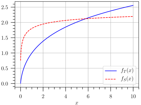
Figure 2: Loop functions $\displaystyle f_{T}(x)$ (solid blue) and $\displaystyle f_{S}(x)$ (dashed red).

We also perform a complete analysis of the phase transition in this model by following our previous work on the $\displaystyle\mathbb{Z}_{2}$ symmetric case, i.e., scalar Higgs portal Beniwal:2017eik and a very recent update on the calculation of the phase transition dynamics Ellis:2018mja. In particular, we find the percolation temperature $\displaystyle T_{p}$ at which the phase transition truly completes. This is used to compute the GW signals arising from the phase transition, and discuss the potential discovery prospects of the model at current and future GW experiments. For more details, see section 4.

Let us also point out that we only check one of the necessary conditions for a successful EWBG, while other difficulties might still arise. For instance, the standard mechanism of generating a baryon yield requires a sufficiently slow speed of the expanding bubble walls Bodeker:2009qy; Kozaczuk:2015owa; Kurup:2017dzf. We do not compute the bubble wall velocity to check this requirement (in fact, we assume it to be very high) while calculating the GW spectra. While there are mechanisms which could generate the asymmetry even for very fast walls No:2011fi; Caprini:2011uz; Katz:2016adq, we also do not explicitly make sure that other conditions they carry are fulfilled.

3.4 Electroweak precision observables (EWPO)

With an extra scalar, our model can induce corrections to the gauge boson self-energy diagrams. Its effect on the electroweak precision observables (EWPO) can be parametrised by the oblique parameters $\displaystyle S$, $\displaystyle T$ and $\displaystyle U$ Peskin:1991sw. The $\displaystyle\gamma\gamma$ and $\displaystyle\gamma Z$ self-energies ($\displaystyle\Pi_{\gamma\gamma}$ and $\displaystyle\Pi_{\gamma Z}$ respectively) are not modified as the new scalar is electrically neutral. Thus, only the $\displaystyle W$ and $\displaystyle Z$ boson self-energies are subject to corrections.

In our model, the oblique parameters are shifted from their SM values by Baek:2011aa

$$\displaystyle\Delta T \displaystyle=\frac{3}{16\pi s_{W}^{2}}\left[\cos^{2}\alpha\left\{f_{T}\left(\frac{m_{h}^{2}}{m_{W}^{2}}\right)-\frac{1}{c_{W}^{2}}f_{T}\left(\frac{m_{h}^{2}}{m_{Z}^{2}}\right)\right\}+\sin^{2}\alpha\left\{f_{T}\left(\frac{m_{H}^{2}}{m_{W}^{2}}\right)\right.\right.$$

$$\displaystyle\hskip 11.38109pt\left.\left.-\frac{1}{c_{W}^{2}}f_{T}\left(\frac{m_{H}^{2}}{m_{Z}^{2}}\right)\right\}-\left\{f_{T}\left(\frac{m_{h}^{2}}{m_{W}^{2}}\right)-\frac{1}{c_{W}^{2}}f_{T}\left(\frac{m_{h}^{2}}{m_{Z}^{2}}\right)\right\}\right],$$ (39)

$$\displaystyle\Delta S \displaystyle=\frac{1}{2\pi}\left[\cos^{2}\alpha f_{S}\left(\frac{m_{h}^{2}}{m_{Z}^{2}}\right)+\sin^{2}\alpha f_{S}\left(\frac{m_{H}^{2}}{m_{Z}^{2}}\right)-f_{S}\left(\frac{m_{h}^{2}}{m_{Z}^{2}}\right)\right],$$ (40)

$$\displaystyle\Delta U \displaystyle=\frac{1}{2\pi}\left[\cos^{2}\alpha f_{S}\left(\frac{m_{h}^{2}}{m_{W}^{2}}\right)+\sin^{2}\alpha f_{S}\left(\frac{m_{H}^{2}}{m_{W}^{2}}\right)-f_{S}\left(\frac{m_{h}^{2}}{m_{W}^{2}}\right)\right]-\Delta S,$$ (41)

where $\displaystyle\Delta\mathcal{O}\equiv\mathcal{O}-\mathcal{O}_{\textnormal{SM}}$ for $\displaystyle\mathcal{O}\in(S,T,U)$, $\displaystyle m_{W}\,(m_{Z})$ is the $\displaystyle W\,(Z)$ boson mass, $\displaystyle c_{W}^{2}=m_{W}^{2}/m_{Z}^{2}$ and $\displaystyle s_{W}^{2}=1-c_{W}^{2}$. The loop functions $\displaystyle f_{T}(x)$ and $\displaystyle f_{S}(x)$ are given by Grimus:2008nb

$$\displaystyle f_{T}(x) \displaystyle=\frac{x\log x}{x-1},$$ (42)

$$\displaystyle f_{S}(x) \displaystyle=\begin{dcases}\frac{1}{12}\left[-2x^{2}+9x+\left((x-3)\left(x^{2}-4x+12\right)+\frac{1-x}{x}\right)f_{T}(x)\right.\\ \left.+2\sqrt{(4-x)x}\left(x^{2}-4x+12\right)\tan^{-1}\left(\sqrt{\frac{4-x}{x}}\right)\right],\quad 0<x<4,\\ \frac{1}{12}\left[-2x^{2}+9x+\left((x-3)\left(x^{2}-4x+12\right)+\frac{1-x}{x}\right)f_{T}(x)\right.\\ \left.+\sqrt{(x-4)x}\left(x^{2}-4x+12\right)\log\left(\frac{x-\sqrt{(x-4)x}}{x+\sqrt{(x-4)x}}\right)\right],\quad x\geq 4.\end{dcases}$$ (43)

These are also plotted in Fig. 2. From Eqs. (39)–(41), it is evident that

$$\Delta\mathcal{O}=(1-\cos^{2}\alpha)\Big{[}\mathcal{O}_{\textnormal{SM}}(m_{H})-\mathcal{O}_{\textnormal{SM}}(m_{h})\Big{]}.$$ (44)

Thus, for large $\displaystyle m_{H}$, $\displaystyle\alpha\sim 0,\,\pi$ is required, whereas large mixing angles are compatible with the EWPO constraint provided $\displaystyle m_{H}\sim m_{h}$.

Using the SM reference as $\displaystyle m_{h}^{\textnormal{ref}}=125$ GeV and $\displaystyle m_{t}^{\textnormal{ref}}=172.5$ GeV, the most recent global electroweak fit gives Haller:2018nnx

$$\Delta S=0.04\pm 0.11,\quad\Delta T=0.09\pm 0.14,\quad\Delta U=-0.02\pm 0.11,$$ (45)

and the following correlation matrix

$$\rho_{ij}=\begin{pmatrix}1&0.92&-0.68\\ 0.92&1&-0.87\\ -0.68&-0.87&1\\ \end{pmatrix}.$$ (46)

To constrain the model parameter space from the EWPO, we use the following likelihood function Profumo:2014opa

$$\ln\mathcal{L}_{\textnormal{EWPO}}(\bm{\theta})=-\frac{1}{2}\Delta\chi^{2}=-\frac{1}{2}\sum_{i,\,j}(\Delta\mathcal{O}_{i}-\overline{\Delta\mathcal{O}}_{i})\left(\Sigma^{2}\right)_{ij}^{-1}(\Delta\mathcal{O}_{j}-\overline{\Delta\mathcal{O}}_{j}),$$ (47)

where $\displaystyle\overline{\Delta\mathcal{O}}_{i}$ denotes the central values for the shifts in Eq. (45), $\displaystyle\Sigma_{ij}^{2}\equiv\sigma_{i}\rho_{ij}\sigma_{j}$ is the covariance matrix, $\displaystyle\rho_{ij}$ is the correlation matrix in Eq. (46) and $\displaystyle\sigma_{i}$ are the associated errors in Eq. (45).

3.5 Higgs searches at colliders

Due to a mixing between the interaction eigenstates $\displaystyle(\varphi,s)$, the coupling strengths between the mass eigenstates $\displaystyle(h,H)$ and SM particles are modified with respect to the SM expectation. The effective squared couplings of $\displaystyle(h,H)$ to SM particles are Li:2014wia

$$\left(\frac{g_{h\mathcal{X}\overline{\mathcal{X}}}}{g_{h\mathcal{X}\overline{\mathcal{X}}}^{\textnormal{SM}}}\right)^{2}=\cos^{2}\alpha,\quad\left(\frac{g_{H\mathcal{X}\overline{\mathcal{X}}}}{g_{H\mathcal{X}\overline{\mathcal{X}}}^{\textnormal{SM}}}\right)^{2}=\sin^{2}\alpha,$$ (48)

where $\displaystyle\mathcal{X}$ refers to a SM quark, lepton or gauge boson, and $\displaystyle g_{h\mathcal{X}\overline{\mathcal{X}}}^{\textnormal{SM}}$ $\displaystyle(g_{H\mathcal{X}\overline{\mathcal{X}}}^{\textnormal{SM}})$ are the coupling strengths for a SM-like Higgs boson with mass $\displaystyle m_{h}\,(m_{H})$. For the loop-induced processes, the effective squared couplings are given by Djouadi:2005gi

$$\left(\frac{g_{h\mathcal{Y}\overline{\mathcal{Y}}}}{g_{h\mathcal{Y}\overline{\mathcal{Y}}}^{\textnormal{SM}}}\right)^{2}=\frac{\Gamma_{h\rightarrow\mathcal{Y}\overline{\mathcal{Y}}}}{\Gamma_{h\rightarrow\mathcal{Y}\overline{\mathcal{Y}}}^{\textnormal{SM}}}=\cos^{2}\alpha,\quad\left(\frac{g_{H\mathcal{Y}\overline{\mathcal{Y}}}}{g_{H\mathcal{Y}\overline{\mathcal{Y}}}^{\textnormal{SM}}}\right)^{2}=\frac{\Gamma_{H\rightarrow\mathcal{Y}\overline{\mathcal{Y}}}}{\Gamma_{H\rightarrow\mathcal{Y}\overline{\mathcal{Y}}}^{\textnormal{SM}}}=\sin^{2}\alpha,$$ (49)

where $\displaystyle\mathcal{Y}\overline{\mathcal{Y}}\in(\gamma\gamma,\,\gamma Z,\,gg,\,ggZ)$ and $\displaystyle\Gamma_{h\rightarrow\mathcal{Y}\overline{\mathcal{Y}}}^{\textnormal{SM}}$ $\displaystyle(\Gamma_{H\rightarrow\mathcal{Y}\overline{\mathcal{Y}}}^{\textnormal{SM}})$ are the decay rates for a SM-like Higgs boson with mass $\displaystyle m_{h}\,(m_{H})$. With modified branching ratios of $\displaystyle h/H$ into SM particles, the scalar sector of our model can be constrained using the direct Higgs searches performed at the lepton (e.g., LEP) and hadron (e.g., Tevatron, LHC) colliders.

To constrain the model parameter space from the direct Higgs searches performed at the LEP, Tevatron and the LHC, we use the HiggsBounds_v4.3.1 Bechtle:2013wla package. From the model predictions for the two scalar masses, total decay widths, branching ratios, and effective squared couplings defined in Eqs. (48) and (49), HiggsBounds computes and compares the predicted signal rates for the search channels considered in multiple experimental analyses. By comparing the predicted signal rates against the expected and observed cross-section limits from the direct Higgs searches, it determines whether or not a given parameter point is excluded at 95$\displaystyle\%$ C.L..

For the two physical scalars $\displaystyle(h,H)$, the signal strengths are given by Li:2014wia

$$\displaystyle\mu_{h}=\frac{\Gamma_{h}^{\textnormal{SM}}\cos^{4}\alpha}{\Gamma_{h}^{\textnormal{SM}}\cos^{2}\alpha+\Gamma_{h\rightarrow\overline{\psi}\psi}+\Gamma_{h\rightarrow HH}},$$ (50)

$$\displaystyle\mu_{H}=\frac{\Gamma_{H}^{\textnormal{SM}}\sin^{4}\alpha}{\Gamma_{H}^{\textnormal{SM}}\sin^{2}\alpha+\Gamma_{H\rightarrow\overline{\psi}\psi}+\Gamma_{H\rightarrow hh}}.$$ (51)

In the absence of invisible and cross Higgs decay modes, $\displaystyle\mu_{h}$ $\displaystyle(\mu_{H})$ scales as $\displaystyle\cos^{2}\alpha$ $\displaystyle(\sin^{2}\alpha)$. However, when these decay modes are kinematically allowed, they suppress the $\displaystyle h/H$ signal strength with respect to the SM expectation. Thus, the scalar sector of our model can also be constrained using the Higgs signal strength and mass measurements performed at the LHC.

Experiment	Channel	Obs. signal strength	Ref.
ATLAS	$\displaystyle h\rightarrow WW^{*}$	$\displaystyle 1.18_{-0.21}^{+0.24}$	Aad:2015gba
ATLAS	$\displaystyle h\rightarrow ZZ^{*}$	$\displaystyle 1.46_{-0.34}^{+0.40}$	Aad:2015gba
ATLAS	$\displaystyle h\rightarrow\gamma\gamma$	$\displaystyle 1.17_{-0.26}^{+0.28}$	Aad:2015gba
ATLAS	$\displaystyle h\rightarrow\tau^{+}\tau^{-}$	$\displaystyle 1.44_{-0.37}^{+0.42}$	Aad:2015gba
ATLAS	$\displaystyle h\rightarrow b\overline{b}$	$\displaystyle 0.63_{-0.37}^{+0.39}$	Aad:2015gba
CMS	$\displaystyle h\rightarrow WW^{*}$	$\displaystyle 0.72_{-0.18}^{+0.20}$	Chatrchyan:2013iaa
CMS	$\displaystyle h\rightarrow ZZ^{*}$	$\displaystyle 0.93_{-0.25}^{+0.29}$	Chatrchyan:2013mxa
CMS	$\displaystyle h\rightarrow\gamma\gamma$	$\displaystyle 1.14_{-0.23}^{+0.26}$	Khachatryan:2014ira
CMS	$\displaystyle h\rightarrow\tau^{+}\tau^{-}$	$\displaystyle 0.78_{-0.27}^{+0.27}$	Chatrchyan:2014vua
CMS	$\displaystyle h\rightarrow b\overline{b}$	$\displaystyle 1.00_{-0.50}^{+0.50}$	Chatrchyan:2014vua

Table 2: A summary of Higgs boson signal strength measurements that are included in our analysis. For more details, see Expt_tables/latestresults-1.4.0-LHCinclusive/ directory of HiggsSignals_v1.4.0 Bechtle:2013xfa.

To constrain the model parameter space from the Higgs signal strength and mass measurements, we use the HiggsSignals_v1.4.0 Bechtle:2013xfa package. Assuming a Gaussian probability density function (p.d.f.) for the two scalar masses, we compute a chi-square $\displaystyle\chi_{\textnormal{HS}}^{2}$ using the peak-centered method. In this method, $\displaystyle\chi_{\textnormal{HS}}^{2}$ is evaluated by assigning, for each signal (or peak) observed in multiple experimental analyses (see Table 2), a combination of the two Higgs bosons from our model provided their masses lie within the experimental resolution of an analysis Stal:2013hwa. Following the assignment, a $\displaystyle\chi^{2}_{\mu}$ is evaluated by comparing the signal strength measurement for the peak to the model predicted signal strength. When a mass measurement is also available (e.g., from channels with a good mass-resolution such as the $\displaystyle h\rightarrow\gamma\gamma$ decay mode), a corresponding $\displaystyle\chi^{2}_{m}$ is also evaluated by comparing the model predicted and observed Higgs boson mass. Thus, the total $\displaystyle\chi_{\textnormal{HS}}^{2}$ is given by

$$\chi_{\textnormal{HS}}^{2}=\chi_{\mu}^{2}+\chi^{2}_{m}=\chi^{2}_{\mu}+\sum_{i=1}^{2}\chi_{m_{i}}^{2}.$$ (52)

In situations where more than one Higgs boson can contribute to a signal (as in our case), an optimal assignment of the Higgs bosons to the signals is achieved by minimising the overall $\displaystyle\chi^{2}_{\textnormal{HS}}$. The predicted signal strengths of the two scalars are added incoherently, assuming negligible interference effects. Finally, the computed $\displaystyle\chi_{\textnormal{HS}}^{2}$ is used to define a Higgs signal strength log-likelihood as

$$\ln\mathcal{L}_{\textnormal{HS}}(\bm{\theta})=-\frac{1}{2}\chi_{\textnormal{HS}}^{2}.$$ (53)

Thus, a large $\displaystyle\chi_{\textnormal{HS}}^{2}$ indicates a large deviation between the model predicted signal strength and the best-fit value for a fixed Higgs boson mass, and vice versa.

4 Results

We perform scans of our 7D model parameter space using Diver_v1.0.4 Workgroup:2017htr with lambdajDE = true, NP = 50,000 and convthresh = 10${}^{-5}$. To efficiently sample all parts of the parameter space (even the degenerate ones), we also run several targeted scans and combine the output chains to obtain high-quality profile likelihood (PL) plots.

We present our model results in the form of 1- and 2-dimensional PL plots. For a model parameter $\displaystyle\theta_{i}$ where $\displaystyle i=1,\ldots,7$, a 1D PL $\displaystyle\mathcal{L}_{\textnormal{PL}}(\theta_{i})$ is defined as

$$\mathcal{L}_{\textnormal{PL}}(\theta_{i})\equiv\underset{\{\theta_{j}|\,j\,\neq\,i\}}{\textnormal{max}}\,\mathcal{L}(\bm{\theta}).$$ (54)

Thus, $\displaystyle\mathcal{L}_{\textnormal{PL}}(\theta_{i})$ is a function of $\displaystyle\theta_{i}$ only, i.e., all other parameters are profiled out. Similarly, a 2D PL $\displaystyle\mathcal{L}_{\textnormal{PL}}(\theta_{i},\theta_{j})$ is defined as

$$\mathcal{L}_{\textnormal{PL}}(\theta_{i},\theta_{j})\equiv\underset{\{\theta_{k}|\,k\,\neq\,i,\,j\}}{\textnormal{max}}\,\mathcal{L}(\bm{\theta}).$$ (55)

Thus, $\displaystyle\mathcal{L}_{\textnormal{PL}}(\theta_{i},\theta_{j})$ is a function of $\displaystyle\theta_{i}$ and $\displaystyle\theta_{j}$ only. Using Eqs. (54) and (55), we can define a PL ratio Cowan:2010js as

$$\Lambda(\theta_{i})=\frac{\mathcal{L}_{\textnormal{PL}}(\theta_{i})}{\mathcal{L}(\hat{\bm{\theta}})},\quad\Lambda(\theta_{i},\theta_{j})=\frac{\mathcal{L}_{\textnormal{PL}}(\theta_{i},\theta_{j})}{\mathcal{L}(\hat{\bm{\theta}})},$$ (56)

where $\displaystyle\hat{\bm{\theta}}\equiv(\hat{\theta}_{1},\ldots,\hat{\theta}_{7})$ is the best-fit point, i.e., a parameter point that maximises the total likelihood function $\displaystyle\mathcal{L}(\bm{\theta})$. Using Wilks’ theorem Wilks:1938dza, Eq. (56) can be used to construct $\displaystyle 1\sigma$ $\displaystyle(2\sigma)$ contours corresponding to $\displaystyle\sim 68.3\%\,(95.4\%)$ C.L. regions.

In the following subsections, we present our model results in the form of 1D and 2D PL plots. These are generated using the pippi_v2.0 Scott:2012qh package.

4.1 EWBG only

We start by finding regions in the model parameter space where a successful EWBG is potentially viable. This is achieved by performing a 7D scan of the model using only the $\displaystyle v_{c}/T_{c}$ log-likelihood, i.e.,

$$\ln\mathcal{L}(\bm{\theta})=\ln\mathcal{L}_{v_{c}/T_{c}}(\bm{\theta}),$$ (57)

where $\displaystyle\ln\mathcal{L}_{v_{c}/T_{c}}(\bm{\theta})$ is defined in subsection 3.3. The resulting 2D PL plots are shown in Fig. 3. In the dark blue regions where the PL ratio $\displaystyle\Lambda\equiv\mathcal{L}/\mathcal{L}_{\textnormal{max}}=1$, the dimensionless parameter $\displaystyle v_{c}/T_{c}\geq 0.6$ and a successful EWBG can be viable. To understand the results in more detail, we go over each panel in Fig. 3 one-by-one.

1. $\displaystyle(m_{H},s_{0})$ plane: For $\displaystyle m_{H}\lesssim 1.3$ TeV, all values of $\displaystyle s_{0}$ and some combination of 5 profiled out parameters (namely $\displaystyle\mu_{3}$, $\displaystyle\lambda_{S}$, $\displaystyle\alpha$, $\displaystyle m_{\psi}$ and $\displaystyle g_{S}$) give $\displaystyle v_{c}/T_{c}\geq 0.6$ and maximise the $\displaystyle v_{c}/T_{c}$ log-likelihood, thus $\displaystyle\Lambda=1$ everywhere. Due to the dependence of $\displaystyle s_{0}$ in Eq. (22), large values of $\displaystyle|s_{0}|$ should lead to runaway directions, $\displaystyle\lambda_{\Phi S}\leq-2\sqrt{\lambda_{\Phi}\lambda_{S}}$, and/or non-perturbative coupling, $\displaystyle|\lambda_{\Phi S}|\geq 4\pi$. With $\displaystyle\alpha=\pi/2$, a large contribution from $\displaystyle m_{H}$ to $\displaystyle\lambda_{\Phi S}$ can be suppressed. However, this choice of $\displaystyle\alpha$ makes $\displaystyle\lambda_{\Phi}$ in Eq. (20) non-perturbative as its contribution appears as $\displaystyle m_{H}^{2}\sin^{2}\alpha$. Ultimately, the solution is to choose a small value for $\displaystyle\lambda_{S}$ as its contribution in Eq. (22) appears as $\displaystyle-\lambda_{S}s_{0}^{2}$. In addition, small values of $\displaystyle\mu_{3}$ can also help in keeping $\displaystyle|\lambda_{\Phi S}|<4\pi$. Thus, for $\displaystyle m_{H}\lesssim 1.3$ TeV, large values of $\displaystyle|s_{0}|$ can facilitate EWBG.

   For $\displaystyle m_{H}\gtrsim 1.3$ TeV and $\displaystyle|s_{0}|\gtrsim 50$ GeV, the white region ($\displaystyle\Lambda=0$) is disfavoured as it leads to $\displaystyle|\lambda_{\Phi S}|\geq 4\pi$. This is expected as the contribution from $\displaystyle m_{H}$ in Eq. (22) is dominant at large values. With large $\displaystyle|s_{0}|$, no choice of $\displaystyle\mu_{3}$, $\displaystyle\lambda_{S}$ and $\displaystyle\alpha$ can keep $\displaystyle|\lambda_{\Phi S}|<4\pi$. In fact, the requirement $\displaystyle|\lambda_{\Phi S}|<4\pi$ translates into an upper limit on $\displaystyle m_{H}$ as a function of $\displaystyle s_{0}$, $\displaystyle\mu_{3}$, $\displaystyle\lambda_{S}$ and $\displaystyle\alpha$. Using Eq. (22), we get

   $$\frac{v_{0}}{s_{0}}(m_{H}^{2}-m_{h}^{2})\sin 2\alpha+4(m_{h}^{2}\sin^{2}\alpha+m_{H}^{2}\cos^{2}\alpha+\mu_{3}s_{0}-2\lambda_{S}s_{0}^{2})<8\pi v_{0}^{2}.$$ (58)

   For a fixed $\displaystyle m_{H}$ and $\displaystyle s_{0}$, Eq. (58) has 3 degrees of freedom. As $\displaystyle\mu_{3}$, $\displaystyle\lambda_{S}$ and $\displaystyle\alpha$ are profiled over, it is non-trivial to predict the exact shape of the upper limit on $\displaystyle m_{H}$ as a function of $\displaystyle s_{0}$. The upper limit also weakens as $\displaystyle|s_{0}|$ increases. The net result is that for $\displaystyle m_{H}\gtrsim 5$ TeV, $\displaystyle|s_{0}|\lesssim 50$ GeV is required to facilitate EWBG.

2. $\displaystyle(m_{H},\alpha)$ plane: Similar to the $\displaystyle(m_{H},s_{0})$ plane for $\displaystyle m_{H}\lesssim 1.3$ TeV, some combination of the profiled out parameters gives $\displaystyle v_{c}/T_{c}\geq 0.6$ for all values of $\displaystyle\alpha$. However, when $\displaystyle m_{H}\gtrsim 1.3$ TeV and $\displaystyle\alpha\neq 0,\,\pi$, the Higgs quartic coupling $\displaystyle\lambda_{\Phi}$ in Eq. (20) becomes non-perturbative. In fact, the requirement $\displaystyle|\lambda_{\Phi}|<4\pi$ translates into the following upper limit on $\displaystyle m_{H}$ as a function of $\displaystyle\alpha$

   $$m_{H}^{2}\sin^{2}\alpha<8\pi v_{0}^{2}-m_{h}^{2}\cos^{2}\alpha.$$ (59)

   When $\displaystyle\alpha=0,\,\pi$, the above condition is satisfied for all values of $\displaystyle m_{H}$. Thus, a successful EWBG can be viable at large values of $\displaystyle m_{H}$. On the other hand, when $\displaystyle\alpha=\pi/2$, Eq. (59) imposes the strongest upper limit on $\displaystyle m_{H}$, namely $\displaystyle m_{H}\lesssim 1.23$ TeV. As $\displaystyle\alpha\rightarrow 0,\,\pi$, the upper limit on $\displaystyle m_{H}$ becomes weaker, as is evident from the plot.

3. $\displaystyle(m_{H},\mu_{3})$ and $\displaystyle(m_{H},\lambda_{S})$ planes: In these two planes, all possible combinations of $\displaystyle(m_{H},\mu_{3})$, $\displaystyle(m_{H},\lambda_{S})$ and profiled out parameters give $\displaystyle v_{c}/T_{c}\geq 0.6$. Thus, the PL ratio is roughly flat and equal to 1 everywhere; hence, we do not show these planes in Fig. 3. In fact, the $\displaystyle v_{c}/T_{c}$ likelihood is weakly dependent on $\displaystyle\mu_{3}$ and $\displaystyle\lambda_{S}$ as expected from Eq. (22). For instance, at large values of $\displaystyle\mu_{3}$ or $\displaystyle\lambda_{S}$ which would give $\displaystyle|\lambda_{\Phi S}|\geq 4\pi$ or $\displaystyle\lambda_{\Phi S}\leq-2\sqrt{\lambda_{\Phi}\lambda_{S}}$, small values of $\displaystyle s_{0}$ can be chosen to avoid such situations.

4. $\displaystyle(m_{H},m_{\psi})$ plane: For $\displaystyle m_{H}\lesssim 5$ TeV, all values of $\displaystyle m_{\psi}$ give $\displaystyle v_{c}/T_{c}\geq 0.6$. As $\displaystyle m_{\psi}$ does not appear directly in Eqs. (20) and (22), the $\displaystyle v_{c}/T_{c}$ likelihood is weakly dependent on $\displaystyle m_{\psi}$. This is expected as the contribution from $\displaystyle m_{\psi}$ to the effective potential appears only at 1-loop order.

   

   

   

   

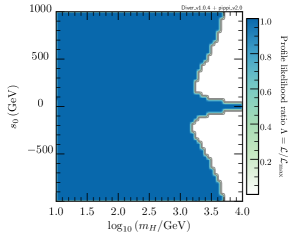
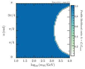
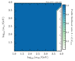
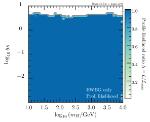
   Figure 3: 2D profile likelihood (PL) plots from a 7D scan of our model using only the electroweak baryogenesis (EWBG) constraint. The contour lines mark out the $\displaystyle 1\sigma$ (68.3$\displaystyle\%$) and $\displaystyle 2\sigma$ (95.4$\displaystyle\%$) C.L. regions. In regions where $\displaystyle\Lambda\equiv\mathcal{L}/\mathcal{L}_{\textnormal{max}}=1$, a successful EWBG can be viable as $\displaystyle v_{c}/T_{c}\geq 0.6$ (see text for more details). The parameter planes $\displaystyle(m_{H},\mu_{3})$ and $\displaystyle(m_{H},\lambda_{S})$ are not shown as they are unconstrained by the EWBG constraint.

   For $\displaystyle m_{H}\gtrsim 5$ TeV and $\displaystyle m_{\psi}\lesssim 3.2$ TeV, no combination of the profiled out parameters can keep $\displaystyle|\lambda_{\Phi S}|<4\pi$. On the other hand, when $\displaystyle m_{\psi}\gtrsim 3.2$ TeV, one can arrange for a cancellation of large quantum corrections to obtain perturbative couplings, although all such solutions carry some degree of extra tuning.

5. $\displaystyle(m_{H},g_{S})$ plane: For $\displaystyle g_{S}\lesssim 5.62$, all values of $\displaystyle m_{H}$ and profiled out parameters give $\displaystyle v_{c}/T_{c}\geq 0.6$, and maximise the $\displaystyle v_{c}/T_{c}$ likelihood. However, values of $\displaystyle g_{S}>5.62$ lead to runaway directions in the potential as the contribution from $\displaystyle g_{S}$ in the 1-loop corrections become large.

In summary, it is not difficult to facilitate a successful EWBG in our model. For any specific model parameter, usually some combination of the remaining parameters give viable points even if the parameter in question causes problems. For instance, large values of $\displaystyle m_{H}$ generally push up the EWSB minimum and cause it to not become the global minimum at $\displaystyle T=0$. However, this effect can be counteracted by choosing a large value for $\displaystyle m_{\psi}$ which gives a large negative contribution to the effective potential. One exception is $\displaystyle g_{S}>5.62$ which always generates runaway directions in the effective potential. For the remaining model parameters, namely $\displaystyle(m_{H},s_{0},\mu_{3},\lambda_{S},\alpha,m_{\psi})$, the 1D PL ratio $\displaystyle\Lambda$ is roughly flat and equal to 1 for all parameter values. Thus, we do not show the 1D PL plots for our model parameters.

4.2 Global fit

With some intuition on the choice of free model parameters that can facilitate a successful EWBG, we present results from a global fit of our model using the total log-likelihood function in Eq. (3). In practice, we consider two scenarios in which the fermion DM accounts for either a small fraction $\displaystyle(f_{\textnormal{rel}}\leq 1)$ or all $\displaystyle(f_{\textnormal{rel}}=1)$ of the observed DM abundance. In the former case, we use a relic density likelihood that is one-sided Gaussian, whereas in the latter, we use a Gaussian likelihood. For more details, see subsection 3.1.

4.2.1 Scenario I: $\displaystyle f_{\textnormal{rel}}\leq 1$

The resulting 2D PL plots from our 7D scans are shown in Fig. 4. For $\displaystyle m_{H}\lesssim m_{h}/2=62.6$ GeV, the parameter planes are ruled out by the observed Higgs signal strength measurements, EWPO and direct Higgs searches performed at the LEP experiment. As the decay channel $\displaystyle h\rightarrow HH$ is kinematically allowed and dominant in this region for all values of the mixing angle $\displaystyle\alpha$, it reduces the SM-like Higgs signal strength $\displaystyle\mu_{h}$ with respect to SM expectation, see Eq. (50). This translates into a large $\displaystyle\chi^{2}_{\mu}$ in Eq. (53) and is thus disfavoured.

To understand the remaining set of results in more detail, we go over each panel in Fig. 4 one-by-one.

1. $\displaystyle(m_{H},s_{0})$ plane: For $\displaystyle m_{H}\gtrsim 4$ TeV, the parameter planes are ruled out by the EWBG constraint as they either lead to runaway directions, $\displaystyle\lambda_{\Phi S}\leq-2\sqrt{\lambda_{\Phi}\lambda_{S}}$, or non-perturbative couplings, $\displaystyle|\lambda_{\Phi}|,|\lambda_{\Phi S}|\geq 4\pi$. Although, some combinations of the profiled out parameters can give a successful EWBG at large values of $\displaystyle m_{H}$ (see Fig. 3), they are often not compatible with the remaining constraints. This is especially true for the EWPO constraint which only depends on $\displaystyle m_{H}$ and $\displaystyle\alpha$. For large $\displaystyle m_{H}$, $\displaystyle\alpha\simeq 0,\pi$ is required in order to satisfy the EWPO constraint.

   

   

   

   

   

   

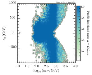
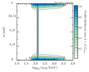
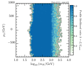
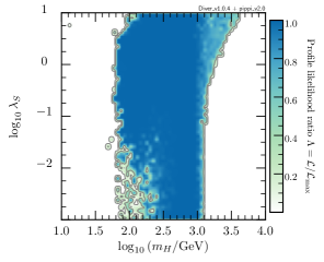
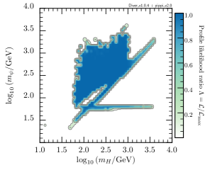
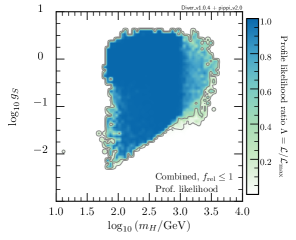
   Figure 4: 2D PL plots from a global fit of our model assuming $\displaystyle f_{\textnormal{rel}}\equiv\Omega_{\psi}/\Omega_{\textnormal{DM}}\leq 1$. The contour lines mark out the $\displaystyle 1\sigma$ (68.3$\displaystyle\%$) and $\displaystyle 2\sigma$ (95.4$\displaystyle\%$) C.L. regions.

2. $\displaystyle(m_{H},\alpha)$ plane: We see that the model is allowed by all constraints for a range of low and high $\displaystyle m_{H}$ values provided $\displaystyle\alpha\simeq 0,\pi$. This is expected as the second scalar $\displaystyle H$ is decoupled in this regime and gives no new contribution to the observed Higgs signal strengths. However, when $\displaystyle m_{H}\simeq m_{h}$, the two scalars are indistinguishable from the point of direct Higgs searches and Higgs signal strength measurements. As is evident in Eqs. (31) and (44), direct detection and EWPO constraints respectively are also relaxed in this regime. The net result is that all values of $\displaystyle\alpha$ are allowed when $\displaystyle m_{H}\simeq m_{h}$.

3. $\displaystyle(m_{H},\mu_{3})$ and $\displaystyle(m_{H},\lambda_{S})$ planes: These parameter planes are mostly unconstrained by our global fit except for $\displaystyle m_{H}\lesssim m_{h}/2$ (excluded by the Higgs signal strength measurements) and $\displaystyle m_{H}\gtrsim 4$ TeV (ruled out by the EWBG constraint). For $\displaystyle m_{H}\gtrsim 1.3$ TeV, large values of $\displaystyle\lambda_{S}$ are required to facilitate a successful EWBG.

4. $\displaystyle(m_{H},m_{\psi})$ plane: For $\displaystyle m_{\psi}\lesssim m_{h}/2$, the fermion DM can only annihilate into light SM quarks, thereby giving $\displaystyle f_{\textrm{rel}}>1$. On the other hand, $\displaystyle m_{\psi}\gtrsim m_{h}/2$ is constrained by the DM relic density and XENON1T limits. When $\displaystyle m_{\psi}\simeq m_{h}/2$, all values of $\displaystyle m_{H}$ up to $\displaystyle\sim 4$ TeV are allowed by the Planck measured relic density and XENON1T limits; this region appears in the plot as a horizontal band. In this band, small values of $\displaystyle g_{S}$ can yield a fermion DM relic density and DM-nucleon cross-section that is compatible with the Planck measured value and XENON1T limit respectively.

   For $\displaystyle m_{\psi}\in[m_{h}/2,m_{H}/2]$, the region is disfavoured by either the Planck measured relic density or XENON1T limit. This is generally expected from an incompatibility between small values of $\displaystyle g_{S}$ which are favoured by the XENON1T limit (as it gives a small DM-nucleon cross-section $\displaystyle\sigma_{\textnormal{SI}}^{\psi\mathcal{N}})$ but disfavoured by the relic density constraint (as it gives $\displaystyle f_{\textnormal{rel}}>1$) and vice versa.

   The diagonal band corresponds to the second resonance $\displaystyle m_{\psi}\simeq m_{H}/2$. Similar to the first resonance $\displaystyle m_{\psi}\simeq m_{h}/2$, all points in this band are allowed by the relic density and XENON1T limits. As $\displaystyle g_{S}$ is profiled over, small values of $\displaystyle g_{S}$ can easily give $\displaystyle f_{\textnormal{rel}}\leq 1$ and $\displaystyle\sigma_{\textnormal{SI}}^{\textnormal{eff}}\leq\sigma_{\textnormal{XENON1T}}$. On the other hand, when $\displaystyle m_{H}\gtrsim 4$ TeV, parameter points are disfavoured by the EWPO and EWBG constraints. For $\displaystyle m_{\psi}\gtrsim 3.2$ TeV, the region is robustly excluded by the combined constraints.

5. $\displaystyle(m_{H},g_{S})$ plane: In this plane, a lower limit on $\displaystyle g_{S}$ comes from the DM relic density constraint as smaller values of $\displaystyle g_{S}$ lead to an overabundance of the fermion DM in the universe today. This lower limit becomes weaker as $\displaystyle m_{H}$ increases. For $\displaystyle m_{H}\gtrsim 4$ TeV, the coupling $\displaystyle\lambda_{\Phi S}$ becomes non-perturbative, thus this region is disfavoured. Similarly, values of $\displaystyle g_{S}\gtrsim 3.2$ are disfavoured by the EWBG constraint as they lead to runaway directions in the potential, see Fig. 3.

In Fig. 5, we show the 1D PL plots for the parameters $\displaystyle m_{H}$, $\displaystyle m_{\psi}$ and $\displaystyle g_{S}$. From these plots, it is evident that the combined constraints impose an upper and lower limit on $\displaystyle m_{H}$, $\displaystyle m_{\psi}$ and $\displaystyle g_{S}$, namely

$$m_{h}/2\lesssim m_{H}\lesssim 5\,\mathrm{TeV},\quad 32\,\mathrm{GeV}\lesssim m_{\psi}\lesssim 3.2\,\mathrm{TeV},\quad 5.6\times 10^{-3}\lesssim g_{S}\lesssim 3.5.$$ (60)

These limits are based on our chosen ranges and priors for the free model parameters (as summarised in Table 1). For instance, our lower limit on $\displaystyle m_{H}$ can be softened by reducing the branching ratio $\displaystyle\mathcal{BR}(h\rightarrow HH)$ when $\displaystyle\alpha=0$, $\displaystyle\pi$. In these cases, the reduced branching ratio can give a better fit to the observed signal strength measurements for a SM-like Higgs boson $\displaystyle h$. For non-zero mixing angles, however, this part of the parameter space is strongly constrained by the direct Higgs searches performed at the LEP experiment.

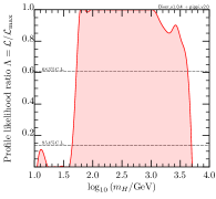
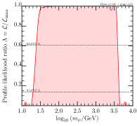
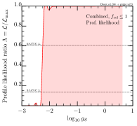
Figure 5: 1D PL plots for $\displaystyle m_{H}$ (left), $\displaystyle m_{\psi}$ (center) and $\displaystyle g_{S}$ (right) assuming $\displaystyle f_{\textnormal{rel}}\leq 1$. The respective plots for $\displaystyle s_{0}$, $\displaystyle\mu_{3}$ and $\displaystyle\lambda_{S}$ are not shown as they are unconstrained by our global fit.

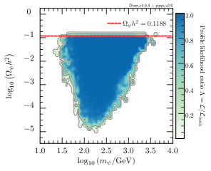
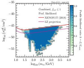
Figure 6: Left panel: Fermion DM relic density vs. the fermion DM mass. The red dashed curve corresponds to the Planck measured value Ade:2015xua. Right panel: Effective SI DM-nucleon cross-section vs. the fermion DM mass. The red dashed curve shows the current 90$\displaystyle\%$ C.L. upper limit from the XENON1T (2018) Aprile:2018dbl, whereas the violet dotted curve shows the projected sensitivity of the LUX-ZEPLIN (LZ) Akerib:2018lyp experiment.

In Fig. 6, we show the key observables such as the fermion DM relic density (left panel) and effective SI DM-nucleon cross-section (right panel). These can be compared against the Planck measured value and XENON1T limit. It is evident that all of the sampled points satisfy $\displaystyle f_{\textnormal{rel}}\leq 1$ and $\displaystyle\sigma_{\textnormal{SI}}^{\textnormal{eff}}\leq\sigma_{\textnormal{XENON1T}}$. We also show the projected sensitivity of the LUX-ZEPLIN (LZ) Akerib:2018lyp experiment. Intriguingly, the LZ experiment will probe 2 orders of magnitude smaller DM-nucleon cross sections than the XENON1T experiment. Due to the two resonances $\displaystyle m_{\psi}\simeq m_{h,H}/2$ and the ability to profile over $\displaystyle\alpha$, the direct detection cross-section in our model can be significantly suppressed to avoid bounds from current and future direct search experiments.

4.2.2 Scenario II: $\displaystyle f_{\textnormal{rel}}=1$

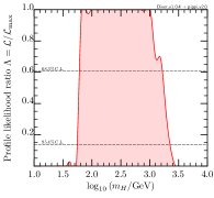
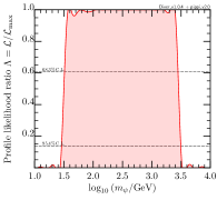
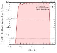
Figure 7: Same as Fig. 5 except for the $\displaystyle f_{\textnormal{rel}}=1$ case.

In this subsection, we present results from our global fit assuming $\displaystyle f_{\textnormal{rel}}=1$. The only difference with respect to the $\displaystyle f_{\textnormal{rel}}\leq 1$ case is our use of a Gaussian likelihood function for the Planck measured DM relic density. In this case, not only small values of $\displaystyle g_{S}$ are disfavoured by the relic density constraint (as they give $\displaystyle f_{\textnormal{rel}}>1$), large values of $\displaystyle g_{S}$ are also disfavoured (as they give $\displaystyle f_{\textnormal{rel}}\ll 1)$.

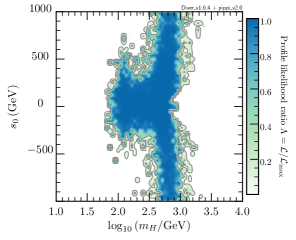
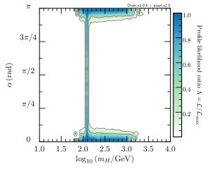
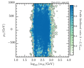
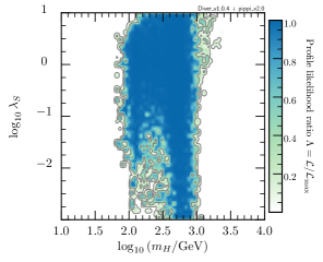
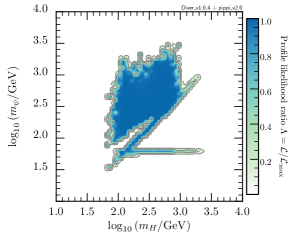
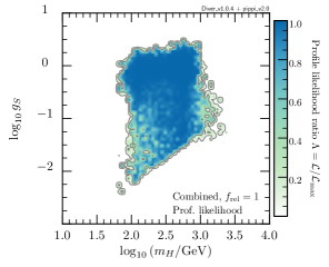
Figure 8: Same as Fig. 4 except for the $\displaystyle f_{\textnormal{rel}}=1$ case.

The resulting 1D and 2D PL plots from our 7D scans are shown in Figs. 7 and 8 respectively. In comparison with Figs. 5 and 4 respectively, the shape of the 1 and 2$\displaystyle\sigma$ C.L. contours is mostly similar; thus we refer to subsection 4.2.1 to avoid repetition. However, the allowed parameter space is significantly smaller. This is expected as the allowed region not only has to reproduce the observed DM abundance, it also has to yield a successful EWBG.

In general, we find that our model can easily satisfy all constraints provided $\displaystyle\alpha\simeq 0$, $\displaystyle\pi$. This is expected as the new scalar $\displaystyle H$ is decoupled in this regime and provides no new contribution to the observed Higgs signal strength measurements. Thus, the allowed final states from the fermion DM annihilation are $\displaystyle hh$, $\displaystyle HH$ and $\displaystyle hH$, which gives $\displaystyle f_{\textnormal{rel}}=1$.

An important point to note is that in the $\displaystyle\mathbb{Z}_{2}$ symmetric case Beniwal:2017eik, the scalar Higgs portal coupling cannot simultaneously explain the observed DM abundance and matter-antimatter asymmetry. This is expected as large values of the portal coupling are required to yield a successful EWBG, whereas small values are required to satisfy the direct detection limits. In contrast, our model contains additional couplings (e.g., $\displaystyle\mu_{3}$ and $\displaystyle\mu_{\Phi S}$) between the new scalar $\displaystyle S$ and SM Higgs boson; these couplings can aid in generating a strong first-order EWPT. As $\displaystyle\mu_{3}$ and $\displaystyle\mu_{\Phi S}$ does not significantly affect the phenomenology of the fermion DM (which is mostly determined by $\displaystyle g_{S}$ and $\displaystyle\alpha$), the fermion DM can easily saturate the observed DM abundance. These two features together allow the model to simultaneously explain the observed DM abundance and matter-antimatter asymmetry.

4.3 Gravitational wave signals

The computation of gravitational wave (GW) signals requires a detailed study of the dynamics of the phase transition (PT). Luckily, the analysis of bubble nucleation is to some extent generic, and the steps required are always similar, albeit using a different scalar potential. In our model, the main difficulty is that the transition always involves both scalar fields, and finding a correct tunnelling path in the 2D field space is always necessary. We tackle this problem in the same way as in Ref. Beniwal:2017eik. In particular, we use the method described there to find the appropriate tunnelling path and the bubble solutions which drive the transition in each case. The main drawback of this calculation is that it is computationally expensive when compared to all other constraints discussed in section 3. Thus, we first identify interesting points in the model parameter space from our global fit, and check the detailed PT dynamics and GW signals afterwards.

For each viable point from our global fit assuming $\displaystyle f_{\textnormal{rel}}\leq 1$, we compute the tunnelling path and corresponding action as in Ref. Beniwal:2017eik. Next, we compute the fraction of volume converted to the true vacuum Ellis:2018mja to accurately calculate the bubble percolation temperature $\displaystyle T_{p}$. This allows us to identify cases in which too strong supercooling renders percolation impossible; as temperature drops, the false vacuum energy dominates the expansion of the universe and an inflationary phase begins Ellis:2018mja; Turner:1992tz; Guth:1982pn. We find that a significant number of interesting points are excluded as the decay is too suppressed and the transition never successfully finishes. This happens because the extended parameter space with respect to the simple scalar potential in Ref. Beniwal:2017eik allows for a formation of a large tree-level barrier which can persist even at $\displaystyle T=0$ and suppress the vacuum decay probability. In our 7D scans, we only use the approximation involving the critical temperature $\displaystyle T_{c}$ at which the symmetric and EWSB minima are degenerate. Such points are perfectly valid and predict $\displaystyle v_{c}/T_{c}>1$ as required for a successful EWBG. However, after a more detailed analysis, we find that roughly $\displaystyle 50\%$ of all points remain viable and their GW spectra have large enough amplitudes to be shown in our plots.

For the viable parameter points, we calculate the ratio of the released latent heat to the energy density of the plasma background, $\displaystyle\alpha_{\rm GW}$, and the size of bubbles carrying the most energy at percolation $\displaystyle R_{\rm MAX}$, which we then convert to the more familiar inverse time of the phase transition $\displaystyle\beta/H=(8\pi)^{1/3}v_{w}/(HR_{\rm MAX})$ Ellis:2018mja; Enqvist:1991xw. These two parameters are essential for computing the GW spectra Grojean:2006bp; Caprini:2015zlo. We also assume that the speed of bubble walls is close to the speed of light $\displaystyle(v_{w}/c\approx 1)$ which is valid for the very strong first-order PTs that we are mostly interested in.

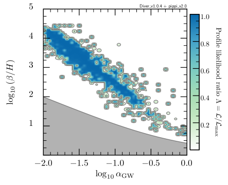
Figure 9: Viable points from our global fit assuming $\displaystyle f_{\textnormal{rel}}\leq 1$ in terms of the parameters $\displaystyle\alpha_{\rm GW}$ and $\displaystyle\beta/H$. The grey region shows where the sound waves last more than a Hubble time (assuming $\displaystyle v_{w}/c\approx 1$ which results in the largest allowed area) and reliably produce a GW signal.

Our calculation of the GW spectrum is based on Ref. Ellis:2018mja. In particular, we do not include the signal contribution from collisions of bubbles Kamionkowski:1993fg; Huber:2008hg; Jinno:2016vai; Jinno:2017fby as the bubbles reach equilibrium with the surrounding plasma and most of the energy is pumped into fluid shells around them Bodeker:2017cim. The two remaining sources are sound waves in the plasma Hindmarsh:2013xza; Hindmarsh:2015qta; Hindmarsh:2016lnk; Hindmarsh:2017gnf and turbulence Caprini:2009yp; Kosowsky:2001xp; Gogoberidze:2007an; Niksa:2018ofa ensuing after the sound waves period. We also check the condition for the sound waves to last more than one Hubble time which was assumed to hold while obtaining the GW spectra in references above. We show this criterion in the $\displaystyle(\alpha_{\rm GW},\,\beta/H)$ plane (see Refs. Ellis:2018mja; Hindmarsh:2017gnf for more details) along with our results in Fig. 9, assuming $\displaystyle v_{w}/c\approx 1$ which results in the largest allowed parameter space. We find that no parameter points are consistent with this criterion. This implies that the standard formula for sound wave spectra Caprini:2015zlo is probably overestimating the true signal. On the other hand, the turbulence signal will be stronger than the standard estimate as the turbulent motion begins more promptly after the PT.

In Fig. 10, we show the resulting GW spectra of viable points as sourced by sound waves (top panel) and turbulence (bottom panel), and their dependence on the percolation temperature $\displaystyle T_{p}$. As the condition to reliably generate a GW signal from sound waves is not fulfilled, a dedicated numerical simulation would be necessary to ascertain the spectral shape. We expect that the final results will lie somewhere between these two figures. In these figures, we discarded points with almost identical GW parameters to avoid plotting many overlapping results. Thus, we only show 100 representative lines out of 10,000 GW spectra as computed from our results. We also show the detection prospects of Laser Interferometer Space Antenna (LISA) Bartolo:2016ami (assuming the most optimistic A5M5 configuration), Deci-hertz Interferometer Gravitational-wave Observatory (DECIGO) and Big Bang Observer (BBO) Yagi:2011wg. The current and future sensitivity bands of LIGO TheLIGOScientific:2014jea; TheLIGOScientific:2016wyq; Thrane:2013oya, the European Pulsar Timing Array (EPTA) vanHaasteren:2011ni, the Square Kilometre Array (SKA) Janssen:2014dka, Cosmic Explorer (CE) Evans:2016mbw and the Einstein Telescope (ET) Punturo:2010zz; Hild:2010id fall in a different frequency range than that of the viable points. Thus, these experiments give no hope for detection of any of our results.

Sound Waves

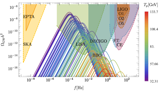
Turbulence

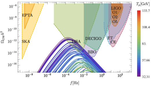
Figure 10: Gravitational wave (GW) spectra of viable points as sourced by sound waves (top panel) and turbulence (bottom panel) along with their dependence on the percolation temperature $\displaystyle T_{p}$. Current sensitivity bands of LIGO and EPTA, as well as detection prospects of LISA, DECIGO, BBO and SKA are also shown for comparison (see text for more details).

In summary, we find that the GW spectra of viable points that are interesting from the point of view of baryogenesis can lie within reach of future GW experiments such as LISA, DECIGO and BBO. However, the uncertainty of the sound wave spectrum can have a dramatic impact on the results. In the overly optimistic case of the standard sound wave signal, roughly $\displaystyle 15\%$ of all of our viable points would be detectable by LISA while for the most pessimistic turbulence-only spectrum, this number falls below half a percent. We also confirm that pulsar timing arrays and terrestrial experiments (e.g., LIGO) are not sensitive to frequencies that result in a GW signal from a strong EWPT. Notably, our results are qualitatively very similar to the $\displaystyle\mathbb{Z}_{2}$ symmetric ones in Ref. Ellis:2018mja, despite our general non-$\displaystyle\mathbb{Z}_{2}$ symmetric potential. This leads us to believe that our current knowledge of the Higgs boson properties (most notably, a constraint on the mixing angle $\displaystyle\alpha$) is enough to significantly constrain viable potentials, and bring them closer to the $\displaystyle\mathbb{Z}_{2}$ symmetric case.

5 Conclusions

In this paper, we have performed the most comprehensive and up-to-date study of the extended scalar singlet model with a fermionic DM candidate. After performing a 7D scan of the model using only the EWBG constraint, we found regions in the model parameter space that can facilitate a successful EWBG. From our 1D PL plots, we showed that a successful EWBG can be viable in all parts of the model parameter space provided $\displaystyle g_{S}\lesssim 5.62$.

After building intuition from the EWBG only results, we performed a global fit of our model using the constraints from the Planck measured DM relic density, direct detection limits from the XENON1T (2018) experiment, electroweak precision observables (EWPO) and Higgs searches at colliders. This allowed us to constrain parts of the 7D model parameter space. In particular, our global fit placed an upper and lower limit on $\displaystyle m_{H}$, $\displaystyle m_{\psi}$ and $\displaystyle g_{S}$, namely $\displaystyle m_{h}/2\lesssim m_{H}\lesssim 5$ TeV, $\displaystyle 32\,\mathrm{GeV}\lesssim m_{\psi}\lesssim 3.2$ TeV and $\displaystyle 5.6\times 10^{-3}\lesssim g_{S}\lesssim 3.5$. Moreover, we confirmed that our model can simultaneously yield a strong first-order phase transition and saturate the observed DM abundance. This is an important feature which is missing in the $\displaystyle\mathbb{Z}_{2}$ symmetric case.

From the viable points that satisfied all of the available constraints, we computed the GW spectra, and checked the discovery prospects of the model at current and future GW experiments. In doing so, we found that the GW spectra of viable points can be within reach of future GW experiments such as LISA, DECIGO and BBO. We checked that the condition for sound waves to be a long-lasting source of GWs is not satisfied for any of our results. This implies that the standard sound wave spectrum used in the literature likely overestimates the true signal, whereas the turbulence signal can be stronger than the standard prediction as the turbulence sets in quicker after the end of the phase transition. Unfortunately, the overall result will still likely be a reduction of the overall spectrum, thereby reducing the discovery prospects. Specifically, in our results we find that $\displaystyle 15\%$ of our viable points would be within the reach of LISA if the final spectrum was close to the standard sound wave prediction. However, this number falls down to less than half a percent in the most pessimistic case of only a turbulence-sourced GW signal.

Appendix A Tree-level scalar potential

The tree-level scalar potential in Eq. (5) expands to

$$V_{\textnormal{tree}}=-\mu_{\Phi}^{2}\Phi^{\dagger}\Phi+\lambda_{\Phi}(\Phi^{\dagger}\Phi)^{2}-\frac{1}{2}\mu_{S}^{2}S^{2}-\frac{1}{3}\mu_{3}S^{3}+\frac{1}{4}\lambda_{S}S^{4}+\mu_{\Phi S}\Phi^{\dagger}\Phi S+\frac{1}{2}\lambda_{\Phi S}\Phi^{\dagger}\Phi S^{2}.$$ (61)

With the following definitions

$$\Phi=\begin{pmatrix}G^{+}\\ \frac{1}{\sqrt{2}}(\phi+iG^{0})\end{pmatrix},\quad\Phi^{\dagger}=\begin{pmatrix}G^{-},&\frac{1}{\sqrt{2}}(\phi-iG^{0})\end{pmatrix},$$

where $\displaystyle G^{-}\equiv(G^{+})^{*}$, the potential in Eq. (61) depends on 2 complex ($\displaystyle G^{+}$, $\displaystyle G^{-}$) and 3 real ($\displaystyle G^{0}$, $\displaystyle\phi$, $\displaystyle S$) scalar fields.

After EWSB, the $\displaystyle\phi$ and $\displaystyle S$ fields acquire their VEVs in Eq. (8). Thus, the following partial derivatives

$$\frac{\partial V_{\textnormal{tree}}}{\partial G^{0}},\,\frac{\partial V_{\textnormal{tree}}}{\partial G^{-}},\,\frac{\partial V_{\textnormal{tree}}}{\partial G^{+}},\,\frac{\partial V_{\textnormal{tree}}}{\partial\phi},\,\frac{\partial V_{\textnormal{tree}}}{\partial S},$$

must vanish at the EWSB minimum $\displaystyle(\left.\langle\phi\rangle\right|_{T=0},\left.\langle S\rangle\right|_{T=0})=(v_{0},s_{0})$. This gives

$$\displaystyle 0 \displaystyle=\left.\frac{\partial V_{\textnormal{tree}}}{\partial G^{0}}\right|_{(v_{0},\,s_{0})}=\left.\frac{\partial V_{\textnormal{tree}}}{\partial G^{-}}\right|_{(v_{0},\,s_{0})}=\left.\frac{\partial V_{\textnormal{tree}}}{\partial G^{+}}\right|_{(v_{0},\,s_{0})},$$

$$\displaystyle 0 \displaystyle=\left.\frac{\partial V_{\textnormal{tree}}}{\partial\phi}\right|_{(v_{0},\,s_{0})}=-\mu_{\Phi}^{2}v_{0}+\lambda_{\Phi}v_{0}^{3}+\mu_{\Phi S}s_{0}v_{0}+\frac{1}{2}\lambda_{\Phi S}v_{0}s_{0}^{2},$$

$$\displaystyle 0 \displaystyle=\left.\frac{\partial V_{\textnormal{tree}}}{\partial S}\right|_{(v_{0},\,s_{0})}=-\mu_{S}^{2}s_{0}-\mu_{3}s_{0}^{2}+\lambda_{S}s_{0}^{3}+\frac{1}{2}\mu_{\Phi S}v_{0}^{2}+\frac{1}{2}\lambda_{\Phi S}s_{0}v_{0}^{2}.$$

A simple rearrangement gives us the following EWSB conditions

$$\displaystyle\mu_{\Phi}^{2} \displaystyle=\lambda_{\Phi}v_{0}^{2}+\mu_{\Phi S}s_{0}+\frac{1}{2}\lambda_{\Phi S}s_{0}^{2},$$ (62)

$$\displaystyle\mu_{S}^{2} \displaystyle=-\mu_{3}s_{0}+\lambda_{S}s_{0}^{2}+\frac{\mu_{\Phi S}v_{0}^{2}}{2s_{0}}+\frac{1}{2}\lambda_{\Phi S}v_{0}^{2}.$$ (63)

Now, we compute the second-order partial derivatives at the EWSB minimum. The only non-zero ones are given by

$$\displaystyle\left.\frac{\partial^{2}V_{\textnormal{tree}}}{\partial G^{0}\,\partial G^{0}}\right|_{(v_{0},\,s_{0})}=\left.\frac{\partial^{2}V_{\textnormal{tree}}}{\partial G^{-}\,\partial G^{+}}\right|_{(v_{0},\,s_{0})} \displaystyle=\left.\frac{\partial^{2}V_{\textnormal{tree}}}{\partial G^{+}\,\partial G^{-}}\right|_{(v_{0},\,s_{0})}=-\mu_{\Phi}^{2}+\lambda_{\Phi}v_{0}^{2}+\mu_{\Phi S}s_{0}+\frac{1}{2}\lambda_{\Phi S}s_{0}^{2},$$

$$\displaystyle\left.\frac{\partial^{2}V_{\textnormal{tree}}}{\partial\phi^{2}}\right|_{(v_{0},\,s_{0})} \displaystyle=-\mu_{\Phi}^{2}+3\lambda_{\Phi}v_{0}^{2}+\mu_{\Phi S}s_{0}+\frac{1}{2}\lambda_{\Phi S}s_{0}^{2},$$

$$\displaystyle\left.\frac{\partial^{2}V_{\textnormal{tree}}}{\partial S^{2}}\right|_{(v_{0},\,s_{0})} \displaystyle=-\mu_{S}^{2}-2\mu_{3}s_{0}+3\lambda_{S}s_{0}^{2}+\frac{1}{2}\lambda_{\Phi S}v_{0}^{2},$$

$$\displaystyle\left.\frac{\partial^{2}V_{\textnormal{tree}}}{\partial\phi\,\partial S}\right|_{(v_{0},\,s_{0})}=\left.\frac{\partial^{2}V_{\textnormal{tree}}}{\partial S\,\partial\phi}\right|_{(v_{0},\,s_{0})} \displaystyle=\mu_{\Phi S}v_{0}+\lambda_{\Phi S}v_{0}s_{0}.$$

Using Eqs. (62) and (63), these expressions can be simplified to

$$\displaystyle\left.\frac{\partial^{2}V_{\textnormal{tree}}}{\partial G^{0}\,\partial G^{0}}\right|_{(v_{0},\,s_{0})}=\left.\frac{\partial^{2}V_{\textnormal{tree}}}{\partial G^{-}\,\partial G^{+}}\right|_{(v_{0},\,s_{0})} \displaystyle=\left.\frac{\partial^{2}V_{\textnormal{tree}}}{\partial G^{+}\,\partial G^{-}}\right|_{(v_{0},\,s_{0})}=0,$$ (64)

$$\displaystyle\left.\frac{\partial^{2}V_{\textnormal{tree}}}{\partial\phi^{2}}\right|_{(v_{0},\,s_{0})} \displaystyle=2\lambda_{\Phi}v_{0}^{2},$$ (65)

$$\displaystyle\left.\frac{\partial^{2}V_{\textnormal{tree}}}{\partial S^{2}}\right|_{(v_{0},\,s_{0})} \displaystyle=-\mu_{3}s_{0}+2\lambda_{S}s_{0}^{2}-\frac{\mu_{\Phi S}v_{0}^{2}}{2s_{0}},$$ (66)

$$\displaystyle\left.\frac{\partial^{2}V_{\textnormal{tree}}}{\partial\phi\,\partial S}\right|_{(v_{0},\,s_{0})}=\left.\frac{\partial^{2}V_{\textnormal{tree}}}{\partial S\,\partial\phi}\right|_{(v_{0},\,s_{0})} \displaystyle=\mu_{\Phi S}v_{0}+\lambda_{\Phi S}v_{0}s_{0}.$$ (67)

After EWSB, the $\displaystyle\phi$ and $\displaystyle S$ fields can be expanded as

$$\phi=v_{0}+\varphi,\quad S=s_{0}+s.$$ (68)

As $\displaystyle\partial V_{\textnormal{tree}}/\partial\phi=\partial V_{\textnormal{tree}}/\partial\varphi$ and $\displaystyle\partial V_{\textnormal{tree}}/\partial S=\partial V_{\textnormal{tree}}/\partial s$, a mass-term for the real scalar fields $\displaystyle\mathcal{A}^{T}=(\varphi,s)$ is

$$\mathscr{L}_{\textnormal{mass--term}}=-\frac{1}{2}\mathcal{A}^{T}\mathcal{M}^{2}\mathcal{A},$$ (69)

where

$$\mathcal{M}^{2}=\begin{pmatrix}\mathcal{M}_{\varphi\varphi}^{2}&\mathcal{M}_{\varphi s}^{2}\\[4.2679pt] \mathcal{M}_{s\varphi}^{2}&\mathcal{M}_{ss}^{2}\end{pmatrix}\equiv\begin{pmatrix}\left.\frac{\partial^{2}V_{\textnormal{tree}}}{\partial\varphi^{2}}\right|_{(v_{0},\,s_{0})}&\left.\frac{\partial^{2}V_{\textnormal{tree}}}{\partial\varphi\,\partial s}\right|_{(v_{0},\,s_{0})}\\[14.22636pt] \left.\frac{\partial^{2}V_{\textnormal{tree}}}{\partial s\,\partial\varphi}\right|_{(v_{0},\,s_{0})}&\left.\frac{\partial^{2}V_{\textnormal{tree}}}{\partial s^{2}}\right|_{(v_{0},\,s_{0})}\end{pmatrix}$$ (70)

is the squared mass matrix. Using Eqs. (65)–(67), the matrix elements are given by

$$\mathcal{M}_{\varphi\varphi}^{2}=2\lambda_{\Phi}v_{0}^{2},\quad\mathcal{M}_{ss}^{2}=-\mu_{3}s_{0}+2\lambda_{S}s_{0}^{2}-\frac{\mu_{\Phi S}v_{0}^{2}}{2s_{0}},\quad\mathcal{M}_{\varphi s}^{2}=\mathcal{M}_{s\varphi}^{2}=\mu_{\Phi S}v_{0}+\lambda_{\Phi S}v_{0}s_{0}.$$ (71)

For the EWSB minimum to be a stable (i.e., not a saddle point) solution of Eq. (61), the symmetric $\displaystyle 5\times 5$ Hessian matrix $\displaystyle\mathcal{H}$ must be positive-definite. At the EWSB minimum, it is given by

$$\mathscr{H}|{}_{(v{}_0,s{}_0)}=\begin{array}{cccccc}& G{}^0& G{}^{-}& G{}^{+}& \varphi & S\\ G{}^0& 0& 0& 0& 0& 0& \\ G{}^{-}& 0& 0& 0& 0& 0& \\ G{}^{+}& 0& 0& 0& 0& 0& \\ \varphi & 0& 0& 0& 2\lambda {}_{\mathrm{\Phi }}v{}_0{}^2& \mu {}_{\mathrm{\Phi }S}v{}_0+\lambda {}_{\mathrm{\Phi }S}v{}_{0}s{}_0\\ S& 0& 0& 0& \mu {}_{\mathrm{\Phi }S}v{}_0+\lambda {}_{\mathrm{\Phi }S}v{}_{0}s{}_0& -\mu {}_{3}s{}_0+2\lambda {}_{S}s{}_0{}^2-\frac{\mu {}_{\mathrm{\Phi }S}v{}_0{}^2}{2s{}_0}\end{array}$$