Evidence for a Large Exomoon Orbiting Kepler-1625b

Short title: Evidence for a Large Exomoon Orbiting Kepler-1625b

One Sentence Summary: Hubble Space Telescope observations show a timing offset and an exomoon-like transit associated with a Jupiter-sized planet.

Abstract: Exomoons are the natural satellites of planets orbiting stars outside our solar system, of which there are currently no confirmed examples. We present new observations of a candidate exomoon associated with Kepler-1625b using the Hubble Space Telescope, to validate or refute the moon’s presence. We find evidence in favor of the moon hypothesis, based on timing deviations and a flux decrement from the star consistent with a large transiting exomoon. Self-consistent photodynamical modeling suggests that the planet is likely several Jupiter masses, while the exomoon has a mass and radius similar to Neptune. Since our inference is dominated by a single but highly precise Hubble epoch, we advocate for future monitoring of the system to check model predictions and confirm repetition of the moon-like signal.

Introduction

The search for exomoons remains in its infancy. To date, there are no confirmed exomoons in the literature, although an array of techniques have been proposed to detect their existence, such as microlensing  (?, ?, ?), direct imaging  (?, ?), cyclotron radio emission  (?), pulsar timing  (?) and transits  (?, ?, ?). The transit method is particularly attractive however since many small planets down to lunar radius have already been detected  (?), and transits afford repeated observing opportunities to further study candidate signals.

Previous searches for transiting moons have established that Galilean-sized moons are uncommon at semimajor axes of 0.1 to 1 astronomical unit (AU)  (?). This result is consistent with theoretical work that has shown that the shrinking Hill sphere  (?) and potential capture into evection resonances  (?) during a planet’s inward migration could efficiently remove primordial moons. Nevertheless, amongst a sample of 284 transiting planets recently surveyed for moons, one planet did show some evidence for a large satellite, Kepler-1625b  (?). The planet is a Jupiter-sized validated world  (?) orbiting a solar-mass star  (?) close to 1 AU in a likely circular path  (?), making it a prime a priori candidate for moons. On this basis, and the hints seen in the three transits observed by Kepler, we requested and were awarded time on the Hubble Space Telescope (HST) to observe a fourth transit expected on 28 to 29 October 2017. In this work, we report on these new observations and their impact on the exomoon hypothesis for Kepler-1625b.

Materials and Methods

Our original analysis was the product of a multiyear survey and thus utilized an earlier version of the processed photometry released by the Kepler Science Operations Center (SOC). In that study  (?), we used the simple aperture photometry (SAP) from SOC pipeline version 9.0  (?), but the most recent and final data release uses version 9.3. In this work we reanalyzed the Kepler data using the revised photometry, which includes updated aperture contamination factors that also affect our analysis. During this process, we also investigated the effect of varying the model used to remove a long-term trend present in the Kepler data.

We detrended the revised Kepler photometry using five independent methods. The first method is the CoFiAM (Cosine Filtering with Autocorrelation Minimization) algorithm  (?) which was the approach used in the original study, since it was specifically designed with exomoon detection in mind. In addition, we considered four other popular approaches: a polynomial fit, a local line fit, a median filter, and a Gaussian process (see the Supplementary Materials for a detailed description of each). The detrended photometry is stable across the different methods (see Fig. 1), with a maximum standard deviation (SD) between any two SAP time series of 250 parts per million (ppm), far below the median formal uncertainty of $\sim 590$ ppm. Although we verified that the Presearch Data Conditioning (PDC) version of the photometry  (?, ?) produces similar results (as evident in Fig. 1), we ultimately only used the five SAP reductions in what follows. We produced a “method marginalized” final time series by taking the median of the $i$th datum across the five methods and propagating the variance between them into a revised uncertainty estimate (see the Supplementary Materials for details). In this way, we produced a robust correction of the Kepler data accounting for differences in model assumptions.

We fit photodynamical models  (?) to the revised Kepler data, using the updated contamination factors from SOC version 9.3, before introducing the new HST data. Bayesian model selection revealed only a modest preference for the moon model, with the Bayes factor ($K$), going from $2\log K=20.4$ in our original study down to just $1.0$ now. Detailed investigation revealed that this is not due to our new detrending approach, as we applied our method marginalized detrending to the original version 9.0 data and recovered a similar result to our original analysis (see the Supplementary Materials for details). Instead, it appeared that the reduced evidence was largely caused by the changes in the SAP photometry going from version 9.0 to 9.3, and to a lesser degree by the new contamination factors. This can be seen in Fig. 1, where the third transit in particular experienced a pronounced change between the two versions, and it was this epoch that displayed the greatest evidence for a moon-like signature in the original analysis.

With a much larger aperture than Kepler, HST is expected to provide several times more precise photometry. Accordingly, the question as to whether Kepler-1625b hosts a large moon should incorporate this new information and in what follows we describe how we processed the HST data and then combined them with the revised Kepler photometry.

HST monitored the transit of Kepler-1625b occurring on 28 to 29 October, 2017 with Wide Field Camera 3 (WFC3). A total of 26 orbits, amounting to some 40 hours, were devoted to observing the event. The observations consisted of one direct image and 232 exposures using the G141 grism, a slitless spectroscopy instrument that projects the star’s spectrum across the charge-coupled device (CCD). This provides spectral information on the target in the near-infrared from about 1.1 to 1.7 $\mu$m. Of these 232 exposures, only three were unusable, as they coincided with the spacecraft’s passage through the South Atlantic Anomaly, at which time HST was forced to use its less-accurate gyroscopic guidance system. Each exposure lasted roughly 5 min, resulting in about 45 min on target per orbit. Images were extracted using standard tools made available by the Science Telescope Space Institute (STScI) and are described in the Supplementary Materials.

Native HST time stamps, recorded in the Modified Julian Date system, were converted to Barycentric Julian Date (BJDUTC) for consistency with the Kepler time stamps. The BJDUTC system accounts for light travel time based on the position of the target and the observer with respect to the solar system barycenter at the time of observation. As the position of HST is constantly changing we set the position of the observer to be the center of the Earth at the time of observation, for which a small discrepancy of $\pm 23$ ms is introduced. This discrepancy can be safely ignored for our purposes.

While the telescope performed nominally throughout the observation, three well-documented sources of systematic error were present in our data that required removal. First, thermal fluctuations due to the spacecraft’s orbit led to clear brightness changes across the entire CCD (sometimes referred to as “breathing”), which were corrected for by subtracting image median fluxes (see the Supplementary Materials for details). After computing an optimal aperture for the target, we observed a strong intra-orbit ramping effect (also known as the “hook”) in the white light curve (see Fig. 2), which has been previously attributed to charge trapping in the CCD  (?, ?). We initially tried a standard parametric approach for correcting these ramps using an exponential function, but found the result to be suboptimal. Instead, we devised a new nonparametric approach described in the Supplementary Materials that substantially outperformed the previous approach.

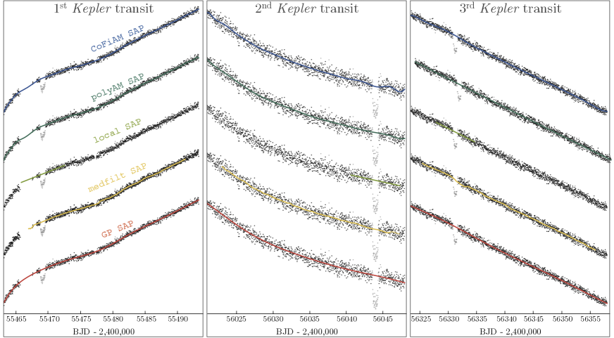
Figure S6: Kepler detrending. Comparison of five different methods used for detrending the SAP Kepler data. Baselines shown represent the full training set used, except for the local method which is trained on only data immediately surrounding the transits of interest.

We achieved a final mean intra-orbit precision of 375.5 ppm (versus 440.1 ppm using exponential functions), which was about 3.8 times more precise than Kepler when correcting for exposure time. The transit of Kepler-1625b was clearly observed even before the hook correction. After removal of the hooks, an apparent second decrease in brightness appeared towards the end of the observations, which was evident even in the noisier exponential ramp corrected data (see Fig. 2). Repeating our analysis for the only other bright star fully on the CCD, KIC 4760469, revealed no peculiar behavior at this time indicating that the dip was not due to an instrumental common mode. Similarly, the centroids of both the target and the comparison star showed no anomalous change around this time (see Fig. S6 in the Supplementary Materials). A detailed analysis of the centroid variations of both the target and the comparison star revealed that the 10 millipixel motion observed was highly unlikely to be able to produce the ${\sim}500$ ppm dip associated with the moon-like signature. Further, we found that the signal was achromatic appearing in two distinct spectral channels, which was consistent with expectations for a real moon. Finally, a detailed analysis of the photometric residuals revealed that the fits including a moon-like transit were consistent with uncorrelated noise equal to the value derived from our hook correction algorithm. These three tests, detailed in the Supplementary Materials, provide no reason to doubt that the moon-like dip is astrophysical in nature and thus we treat it as such in what follows.

Upon inspection of the HST images we identified a previously uncataloged point source within 2 arcseconds of our target. The star resides at position angle 8.5^∘ east of north, with a derived Kepler magnitude of 22.7. We attribute its new identification to the fact that it is both exceptionally faint and so close to the target that it was always lost in the glare in other images. Using a Gaia-derived distance to the target we found that, were this point source to be at the same distance, it would be within 4500 AU of Kepler-1625. However, it is not known whether the two sources are physically associated, however. Its faintness means that it produces negligible contamination to our target spectrum. We estimated that the source has a variability of 0.33% and contributes less than 1 part in 3000 to our final WFC3 white light curve, which means that the net contribution to our target is 1 ppm and can be safely ignored.

In addition to the breathing and the hooks, a third well-known source of WFC3 systematic error we see is a visit-long trend (apparent in Fig. 2). These trends have not yet been correlated to any physical parameter related to the WFC3 observations  (?), and thus the conventional approach is a linear slope (for example, 25-27) although a quadratic model has been used in some instances (for example, 28,29) The time scale of the variations is comparable to the transit itself and thus cannot be removed in isolation; rather, any detrending model is expected to be covariant with the transit model. For this reason, it was necessary to perform the detrending regression simultaneous to the transit model fits. We considered three possible trend models; linear, quadratic and exponential. All models include an extra parameter describing a flux offset between the 14^th and 15^th orbits. This is motivated by the fact that the spacecraft performed a full guide star acquisition at the beginning of the 15^th orbit (a new “visit”), and ended up placing the spectrum ${\sim}$0.1 pixels away from where it appeared during the first 14 orbits. Although the white light curve shows no obvious flux change at this time, the reddest channels display substantial shifts motivating this offset term.

Finally, we extracted light curves in nine wavelength bins across the spectrum in an attempt to perform transmission spectroscopy. As a planet transits its host star, the atmosphere may absorb different amounts of light depending on the constituent molecules and their abundances  (?). This makes the planet’s transit depth wavelength-dependent. An accurate measurement of these transit depths not only provides the potential to characterize the atmosphere’s composition; it is also potentially useful in providing an independent measurement of the planet’s mass  (?). While a low surface gravity planet will show very pronounced molecular features and a steep slope at short wavelengths due to Rayleigh scattering, a high surface gravity world will yield a substantially flatter transmission spectrum.

With the HST WFC3 data prepared, we are ready to combine them with the revised Kepler data to regress candidate models and compare them. We considered four different transit models, which, when combined with three different visit-long trend models, leads to a total of 12 models to evaluate. The four transit models here were designated as P, for the planet-only model; T, for a model that fits the observed transit timing variations (TTVs) in the system agnostically; Z, for the zero-radius moon model, which may produce all the gravitational effects of an exomoon without the flux reductions of a moon transit; and M, which is the full planet plus moon model. Models were generated using the LUNA photodynamical software package  (?) and regression was performed via the multimodal nested sampling algorithm MultiNest  (?, ?). For each model, we derived not only the joint a posteriori parameter samples, but also a Bayesian evidence (also known as the marginal likelihood) enabling direct calculation of the Bayes factor between models.

Results

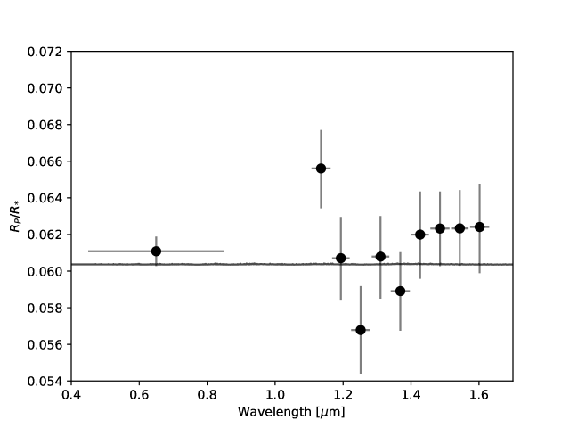
Figure S12: Transmission spectrum. The transmission spectrum measured as the ratio of the planet radius to the stellar radius, utilizing the Kepler bandpass at far left and the spectral channels extracted from the WFC3 grism photometry. For reference a model spectrum assuming $M_{P}=M$_Jup is also plotted.

One clear result from our analysis is that the HST transit of Kepler-1625b occurred 77.8 min earlier than expected, indicating TTVs in the system. Bayes factors between models P and T support the presence of significant TTVs for any choice of detrending model (see Table LABEL:tab:evidences), with the T fits returning a $\chi^{2}$ decreased by 17 to 19 (for 1048 data points). Further, if we fit the Kepler data in isolation and make predictions for the HST transit time, the observed time is $>3$ $\sigma$ discrepant (see Fig. S12 in the Supplementary Materials). For reference, each Kepler transit midtime has an uncertainty on the order of 10 min and the SD on linear ephemeris predictions is 25.2 min derived from posterior samples. Identifying TTVs was among the first methods proposed to discover exomoons  (?), but certainly perturbations from an unseen planet could also be responsible. We find that the ${\simeq}25$ min amplitude TTV can be explained by an external perturbing planet (see the Supplementary Materials), although with only four transits on hand it is not possible to constrain the mass or location of such a planet, and no other planet has been observed so far in the system.

We also found that model Z consistently outperforms model T, though the improvement to the fits is smaller at $\Delta\chi^{2}\simeq 2$-$5$ (see Table LABEL:tab:evidences). This suggests that the evidence for the moon based on timing effects alone goes beyond the TTVs, providing modest evidence in favor of additional dynamical effects such as duration changes  (?) and/or impact parameter variation  (?), both expected consequences of a moon present in the system. This by itself would not constitute a strong enough case for a moon detection claim, but we consider it to be an important additional check that a real exomoon would be expected to pass.

The most compelling piece of evidence for an exomoon would be an exomoon transit, in addition to the observed TTV. If Kepler-1625b’s early transit were indeed due to an exomoon, then we should expect the moon to transit late on the opposite side of the barycenter. The previously mentioned existence of an apparent flux decrease towards the end of our observations is therefore where we would expect it to be under this hypothesis. Although we have established that this dip is most likely astrophysical, we have not yet discussed its significance or its compatibility with a self-consistent moon model.

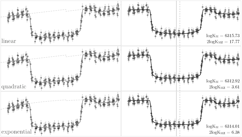
Figure 3: HST detrending. The HST observations with three proposed trends fit to the data (left) and with the trends removed (right). Bottom-right numbers in each row give the Bayes factor between a planet plus moon model (model $\mathrm{M}$) and a planet plus moon model where the moon radius equals zero (model $\mathrm{Z}$), which tracks the significance of the moon-like dip in isolation.

We find that our self-consistent planet plus moon models (M) always outperform all other transit models in terms of maximum likelihood and Bayesian evidences (see Table LABEL:tab:evidences). The moon signal is found to have a signal-to-noise ratio of at least 19. The presence of a TTV and an apparent decrease in flux at the correct phase position together suggest that the exomoon is the best explanation. However, as is apparent from Fig. 3, the amplitude and shape of the putative exomoon transit vary somewhat between the trend models, leading to both distinct model evidences and associated system parameters.

Discussion

Although the overall preference of the moon model is arguably best framed by comparison to model P, the significance of the moon-like transit alone is best framed by comparing M and Z alone. Such a comparison reveals a strong dependency of the implied significance on the trend model used. In the worst case, we have the quadratic model with $2\log K\simeq 4$, corresponding to “positive evidence”  (?) - although we note that the absolute evidence $\mathcal{Z}_{M}$ is the worst amongst the three. The linear model is far more optimistic yielding $2\log K\simeq 18$, corresponding to “very strong evidence”  (?), whereas the exponential sits between these extremes. The question then arises, which of our trend models is the correct one?

Because the linear model is a nested version of the quadratic model, and both models are linear with respect to time, it is more straightforward to compare these two. The quadratic model essentially recovers the linear model, apparent from Fig. 3, with a curvature within 1.5 $\sigma$ of zero, and yields almost the same best $\chi^{2}$ score to within 1.2. This lack of meaningful improvement causes the log evidence to drop by 2.8, since evidences penalize wasted prior volume. The exponential model appears more competitive with a log evidence of 1.72 lower, but a direct comparison of two different classes of models, such as these, is muddied by the fact that these analyses are sensitive to the choice of priors. The most useful comparison here is simply to state that the maximum likelihoods are within $\Delta\chi^{2}=0.68$ of one another and thus are likely equally justified from data-driven perspective.

Another approach we considered is to weigh the trend models using the posterior samples. Given a planet or moon’s mass, there is a probabilistic range of expected radii based on empirical mass-radius relations  (?). Although we exclude extreme densities in our fits, parameters from model M can certainly lead to improbable solutions with regard to the photodynamically inferred  (?) masses and radii.

To investigate this, we inferred the planetary mass using two methods for each model and evaluated their self-consistency. The first method combines the photodynamically-inferred planet-to-star mass ratio  (?) with a prediction for the mass based on the well-constrained radius using forecaster; an empirical probabilistic mass-radius relation  (?). The second method approaches the problem from the other side, taking the moon’s radius and predicting its mass with forecaster and then calculating the planetary mass via the photodynamically-inferred moon-to-planet mass ratio. Our analysis (discussed in more detail in the Supplementary Materials) reveals that all three models have physically plausible solutions and generally converge at ${\sim}10^{3}$ $M_{\oplus}$ for the planetary mass, with the exception of the quadratic model that had broader support extending down to Saturn-mass. We ultimately combined the two mass estimates to provide a final best-estimate for each model in Table LABEL:tab:params.

As a consistency check, we used our derived transmission spectrum to constrain the allowed range of planetary masses for a cloudless atmosphere  (?). Using an MCMC (Markov chain Monte Carlo) with Exo-Transmit  (?), we find that masses in the range of $>0.4$ Jupiter masses (to 95% confidence) are consistent with the nearly flat spectrum observed, assuming a cloudless atmosphere (see the Supplementary Materials for details).

In conclusion, the linear and exponential models appear to be the most justified by the data and also lead to slightly improved physical self-consistency, although we certainly cannot exclude the quadratic model at this time. For this reason, we elected to present the associated system parameters resulting from all three models in Table LABEL:tab:params. The maximum a posteriori solutions from each, using model M, are presented in Fig. 4 for reference.

We briefly comment on some of the inferred physical parameters for this system. First, we have assumed a circular moon orbit throughout due to the likely rapid effects of tidal circularization. However, we did allow the moon to explore three-dimensional orbits and find some evidence for noncoplanarity. Our solution somewhat favors a moon orbit tilted by about 45^∘ to the planet’s orbital plane, with both pro- and retrograde solutions being compatible. The only comparable known large moon with such an inclined orbit is Triton around Neptune, which is generally thought to be a captured Kuiper Belt object  (?). However, we caution that the constraints here are weak, reflected by the posterior’s broad shape, and thus it would be unsurprising if the true answer is coplanar.

One jarring aspect of the system is the sheer scale of it. The exomoon has a radius of ${\simeq}4$ $R_{\oplus}$, making it very similar to Neptune or Uranus in size. The measured mass, including the forecaster constraints, comes in at $\log(M_{S}/M_{\oplus})=(1.2\pm 0.3)$, which is again compatible with Neptune or Uranus (although note that this solution is in part informed by an empirical mass-radius relation). This Neptune-like moon orbits a planet with a size fully compatible with that of Jupiter at $(11.4\pm 1.5)$ $R_{\oplus}$, but most likely a few times more massive. Finally, although the moon’s period is highly degenerate and multimodal, we find the semimajor axis is relatively wide at ${\simeq}40$ planetary radii. With a Hill radius of $(200\pm 50)$ planetary radii, this is well within the Hill sphere and expected region of stability (see the Supplementary Materials for further discussion).

The blackbody equilibrium temperature of the planet and moon, assuming zero albedo, is ${\sim}350$ K. Adopting a more realistic albedo can drop this down to $\sim 300$ K. Of course, as a likely gaseous pair of objects there is not much prospect of habitability here, although it appears that the moon can indeed be in the temperature zone for optimistic definitions of the habitable zone.

What is particularly interesting about the star is that it appears to be a solar-mass star evolving off the main sequence. This inference is supported by a recent analysis of the Gaia DR2 parallax by  (?), as well as our own isochrone fits (see the Supplementary Materials). We find that the star is certainly older than the Sun, at ${\simeq}$9  gigayears in age, and that insolation at the location of the system was thus lower in the past. The luminosity was likely close to solar for most of the star’s life, making the equilibrium temperature drop down to ${\sim}250$ K for Jovian albedos for most of its existence. The old age of the system also implies plenty of time for tidal evolution, which could explain why we find the moon at a fairly wide orbital separation.

The origins of such a system can only be speculated upon at this time. A mass ratio of 1.5% is certainly not unphysical from in-situ formation using gas-starved disk models, but it does represent the very upper end of what numerical simulations form  (?). In such a scenario, a separate explanation for the tilt would be required. Impacts between gaseous planets leading to captured moons are not well-studied but could be worth further investigation. A binary exchange mechanism would be challenged by the requirement for a Neptune to be in an initial binary with an object of comparable mass, such as a super-Earth  (?). Formation of an initial binary planet, perhaps through tidal capture, seems improbable due to the tight orbits simulation work tends to produce from such events  (?). If confirmed, Kepler-1625b-i will certainly provide an interesting puzzle for theorists to solve.

Conclusion

Together, a detailed investigation of a suite of models tested in this work suggests that the exomoon hypothesis is the best explanation for the available observations. The two main pieces of information driving this result are (i) a strong case for TTVs, in particular a 77.8 min early transit observed during our HST observations and (ii) a moon-like transit signature occurring after the planetary transit. We also note that we find a modestly improved evidence when including additional dynamical effects induced by moons aside from TTVs.

The exomoon hypothesis is further strengthened by our analysis that demonstrates that (i) the moon-like transit is not due to an instrumental common mode, residual pixel sensitivity variations, or chromatic systematics; (ii) the moon-like transit occurs at the correct phase position to also explain the observed TTV; and (iii) simultaneous detrending and photodynamical modeling retrieves a solution that is not only favored by the data, but is also physically self-consistent.

Together, these lines of evidence all support the hypothesis of an exomoon orbiting Kepler-1625b. The exomoon is also the simplest hypothesis to explain both the TTV and the post-transit flux decrease, since other solutions would require two separate and unconnected explanations for these two observations.

There remain some aspects of our present interpretation of the data that give us pause. First, the moon’s Neptunian size and inclined orbit are peculiar, though it is difficult to assess how likely this is a priori since no previously known exomoons exist. Second, the moon’s transit occurs towards the end of the observations and more out-of-transit data could have more cleanly resolved this signal. Third, the moon’s inferred properties are sensitive to the model used for correcting HST’s visit-long trend and thus some uncertainty remains regarding the true system properties. However, the solution we deem most likely, a linear visit-long trend, also represents the most widely agreed upon solution for the visit-long trend in the literature.

Finally, it is somewhat ironic that the case for observing Kepler-1625b with HST was contingent on a previous data release of the Kepler photometry that indicated a moon  (?), while the most recent data release only modestly favors that hypothesis when treated in isolation. Despite this, we would argue that planets like Kepler-1625b – Jupiter-sized planets on wide, circular orbits around solar-mass stars – were always ideal targets exomoon follow-up. There are certainly hints of the moon present even in the revised Kepler data, but it is the HST data – with a precision four times superior to Kepler– that are critical to driving the moon as the favored model. These points suggest that it would be worthwhile to pursue similar Kepler planets for exomoons with HST or other facilities, even if the Kepler data alone do not show large moon-like signatures. Furthermore, our work demonstrates how impactful the changes to Kepler photometry were, at least in this case, as it suggests other results over the course of the Kepler mission may be similarly affected, particularly for small signals.

All in all, it is difficult to assign a precise probability to the reality of Kepler-1625b-i. Formally, the preference for the moon model over the planet-only model is very high, with a Bayes factor exceeding 400,000. On the other hand, this is a complicated and involved analysis where a minor effect unaccounted for, or an anomalous artifact, could potentially change our interpretation. In short, it is the unknown unknowns that we cannot quantify. These reservations exist because this would be a first-of-its-kind detection – the first exomoon. Historically, the first exoplanet claims faced great skepticism because there was simply no precedence for them. If many more exomoons are detected in the coming years with similar properties to Kepler-1625b-i, it would hardly be a controversial claim to add one more. Ultimately, Kepler-1625b-i cannot be considered confirmed until it has survived the long scrutiny of many years, observations and community skepticism, and perhaps the detection of similar such objects. Despite this, it is an exciting reminder of how little we really know about distant planetary systems and the great spirit of discovery that exoplanetary science embodies.

Acknowledgements

• We wish to thank STScI staff scientists Bill Januszewski and Kevin Stevenson for their critical contributions during the planning and execution of the HST observation. We also thank Jon Jenkins at NASA and Paul Dalba at Boston University for useful discussions regarding source contamination in the Kepler data. Members of the Cool Worlds Lab at Columbia University (Ruth Angus, Jingjing Chen, Jorge Cortes, Tiffany Jansen, Moiya McTier, Emily Sandford, and Adam Wheeler) provided valuable feedback at every stage of this analysis. We are also grateful to members of the Hunt for Exomoons with Kepler project for their continued support throughout the early years of our program. Finally, we thank Travis Berger and collaborators for sharing their Gaia-derived posteriors for the target’s radius.

• Funding: Analysis was carried out in part on the NASA Supercomputer PLEIADES (grant no. HEC-SMD-17-1386). A.T. is supported through the NSF Graduate Research Fellowship (DGE 16-44869). D.M.K. is supported by the Alfed P. Sloan Foundation Fellowship. This work is based in part on observations made with the NASA/ESA HST, obtained at the Space Telescope Science Institute, which is operated by the Association of Universities for Research in Astronomy, Inc., under NASA contract NAS 5-26555. These observations are associated with program no. GO-15149. Support for program no. GO-15149 was provided by NASA through a grant from the Space Telescope Science Institute, which is operated by the Association of Universities for Research in Astronomy, Inc., under NASA contract NAS 5-26555. This paper includes data collected by the Kepler Mission. Funding for the Kepler Mission was provided by the NASA Science Mission directorate. This research has made use of the Exoplanet Follow-up Observation Program website, which is operated by the California Institute of Technology, under contract with NASA under the Exoplanet Exploration Program.

• Author Contributions: A.T. was responsible for the proposal, planning, and data reduction of the October 2017 HST observation. In addition, A.T. modeled source blending in the Kepler data, investigated the possibility of an external perturbing planet as the source of TTVs, and analyzed the transmission spectrum. D.M.K. led the detrending of the Kepler and HST light curves, and performed the joint fits to the data. D.M.K. also carried out the color, centroid, and residual analyses, as well as the planetary mass inference and isochrone fitting. All aspects of these tasks were executed through joint consultation, and the paper was written collaboratively by the two authors.

• Competing interests: The authors declare that they have no competing interests.

• Data and materials availability: The raw data from both the Kepler and HST observations are freely available for download at the Mikulski Archive for Space Telescopes (https://archive.stsci.edu). All relevant information required for replication of these results and to evaluate the conclusions in the paper are present in the paper and/or the Supplementary Materials. Additional data related to this paper may be requested from the authors. This work made use of Numpy, Scipy, Pandas, Matplotlib, Astropy, TTVfaster, Exo-Transmit, forecaster, LUNA and MultiNest.

List of Supplementary Materials

1. Materials and Methods

2. Tables S1-S3

3. Figures S1-S18

4. References (42-72)

Table 1: Model performance. Bayesian evidences ($\mathcal{Z}$) and maximum likelihoods ($\hat{\mathcal{L}}$) from our combined fits using Kepler and new HST data. Keplerplus HST fits. The subscripts are P for the planet model, T for the planetary TTV model, Z for the zero-radius moon model and M for the moon model. The three columns are for each trend model attempted. The primed values correspond to those derived the Kepler data in isolation.

	linear	quadratic	exponential
$\log\mathcal{Z}_{\mathrm{P}}$	$6302.79\pm 0.11$	$6306.68\pm 0.11$	$6308.41\pm 0.11$
$\log\mathcal{Z}_{\mathrm{T}}$	$6304.86\pm 0.11$	$6308.81\pm 0.12$	$6310.71\pm 0.11$
$\log\mathcal{Z}_{\mathrm{Z}}$	$6306.84\pm 0.11$	$6311.12\pm 0.12$	$6310.82\pm 0.12$
$\log\mathcal{Z}_{\mathrm{M}}$	$6315.73\pm 0.12$	$6312.92\pm 0.12$	$6314.01\pm 0.12$
$2\log K(\mathcal{Z}_{\mathrm{M}}^{\prime}/\mathcal{Z}_{\mathrm{P}}^{\prime})$	$1.00\pm 0.22$
$2\log(\mathcal{Z}_{\mathrm{M}}/\mathcal{Z}_{\mathrm{P}})$	$25.88\pm 0.32$	$12.47\pm 0.33$	$11.19\pm 0.32$
$2\log(\mathcal{Z}_{\mathrm{M}}/\mathcal{Z}_{\mathrm{T}})$	$21.72\pm 0.33$	$8.21\pm 0.34$	$17.81\pm 0.33$
$2\log(\mathcal{Z}_{\mathrm{M}}/\mathcal{Z}_{\mathrm{Z}})$	$17.77\pm 0.33$	$3.61\pm 0.33$	$6.38\pm 0.34$
$\Delta\chi_{\mathrm{PM}}^{\prime 2}=2\log(\hat{\mathcal{L}}_{\mathrm{M}}^{\prime}/\hat{\mathcal{L}}_{\mathrm{P}}^{\prime})$	$18.66$
$\Delta\chi_{\mathrm{PM}}^{2}=2\log(\hat{\mathcal{L}}_{\mathrm{M}}/\hat{\mathcal{L}}_{\mathrm{P}})$	$54.93$	$41.04$	$41.57$
$\Delta\chi_{\mathrm{TM}}^{2}=2\log(\hat{\mathcal{L}}_{\mathrm{M}}/\hat{\mathcal{L}}_{\mathrm{T}})$	$35.69$	$23.97$	$23.97$
$\Delta\chi_{\mathrm{ZM}}^{2}=2\log(\hat{\mathcal{L}}_{\mathrm{M}}/\hat{\mathcal{L}}_{\mathrm{Z}})$	$33.68$	$19.59$	$19.22$

Table 2: System parameters. Median and $\pm 34.1$% quantile range of the a posteriori model parameters from model M, where each column defined a different visit-long trend model. The top panel gives the credible intervals for the actual parameters used in the fit, and the lower panel gives a selection of relevant derived parameters conditioned upon our revised stellar parameters. The quoted inclination of the satellite is the inclination modulo 90^∘.

Parameter	Linear	Quadratic	Exponential
Photodynamics only
$R_{P,\mathrm{Kep}}/R_{\star}$	$0.06075_{-0.00065}^{+0.00062}$	$0.06061_{-0.00073}^{+0.00068}$	$0.06072_{-0.00063}^{+0.0062}$
$R_{P,\mathrm{HST}}/R_{P,\mathrm{Kep}}$	$0.998_{-0.013}^{+0.013}$	$1.009_{-0.017}^{+0.019}$	$1.006_{-0.014}^{+0.014}$
$\rho_{\star,\mathrm{LC}}$ [g cm-3]	$424_{-16}^{+9}$	$424_{-15}^{+9}$	$425_{-14}^{+9}$
$b$	$0.104_{-0.066}^{+0.084}$	$0.099_{-0.063}^{+0.088}$	$0.096_{-0.058}^{+0.078}$
$P_{P}$ [days]	$287.37278_{-0.00065}^{+0.00075}$	$287.3727_{-0.0015}^{+0.0022}$	$287.37269_{-0.00076}^{+0.00074}$
$\tau_{0}$ [BJDUTC]	$2456043.9587_{-0.0027}^{+0.0027}$	$2456043.9572_{-0.0093}^{+0.0033}$	$56043.9585_{-0.0029}^{+0.0025}$
$q_{1,\mathrm{Kep}}$	$0.45_{-0.14}^{+0.19}$	$0.44_{-0.15}^{+0.19}$	$0.45_{-0.14}^{+0.18}$
$q_{2,\mathrm{Kep}}$	$0.31_{-0.15}^{+0.19}$	$0.32_{-0.16}^{+0.20}$	$0.31_{-0.15}^{+0.19}$
$q_{1,\mathrm{HST}}$	$0.087_{-0.041}^{+0.057}$	$0.096_{-0.045}^{+0.064}$	$0.087_{-0.040}^{+0.056}$
$q_{2,\mathrm{HST}}$	$0.25_{-0.15}^{+0.25}$	$0.21_{-0.14}^{+0.23}$	$0.22_{-0.14}^{+0.22}$
$P_{S}$ [days]	$22_{-9}^{+17}$	$24_{-11}^{+18}$	$22_{-9}^{+15}$
$a_{SP}/R_{P}$	$45_{-5}^{+10}$	$36_{-13}^{+10}$	$42_{-4}^{+7}$
$\phi_{S}$ [∘]	$179_{-70}^{+136}$	$141_{-65}^{+161}$	$160_{-60}^{+150}$
$i_{S}$ [∘]	$42_{-18}^{+15}$	$49_{-22}^{+21}$	$43_{-19}^{+15}$
$\Omega_{S}$ [∘]	$0_{-83}^{+142}$	$12_{-113}^{+132}$	$8_{-81}^{+136}$
$(M_{S}/M_{P})$	$0.0141_{-0.0039}^{+0.0048}$	$0.0196_{-0.0071}^{+0.0294}$	$0.0149_{-0.0038}^{+0.0052}$
$(R_{S}/R_{P})$	$0.431_{-0.036}^{+0.033}$	$0.271_{-0.099}^{+0.150}$	$0.363_{-0.079}^{+0.048}$
$\Delta a_{0}$ [ppm]	$330_{-120}^{+120}$	$180_{-210}^{+170}$	$220_{-140}^{+130}$
+ Stellar properties
$R_{\star}$ [$R_{\odot}$]	$1.73_{-0.22}^{+0.24}$	$1.73_{-0.22}^{+0.24}$	$1.73_{-0.22}^{+0.24}$
$M_{\star}$ [$M_{\odot}$]	$1.04_{-0.06}^{+0.08}$	$1.04_{-0.06}^{+0.08}$	$1.04_{-0.06}^{+0.08}$
$\rho_{\star,\mathrm{iso}}$ [kg m-3]	$0.29_{-0.09}^{+0.13}$	$0.29_{-0.09}^{+0.13}$	$0.29_{-0.09}^{+0.13}$
$e_{\mathrm{min}}^{\dagger}$	$0.13_{-0.09}^{+0.11}$	$0.13_{-0.09}^{+0.11}$	$0.13_{-0.09}^{+0.11}$
$R_{P}$ [$R_{\oplus}$]	$11.4_{-1.5}^{+1.6}$	$11.4_{-1.4}^{+1.6}$	$11.4_{-1.4}^{+1.6}$
$\log_{10}(M_{P}/M_{\oplus})$	$2.86_{-0.50}^{+0.48}$	$2.40_{-0.72}^{+0.70}$	$2.75_{-0.54}^{+0.53}$
$a_{P}$ [AU]	$0.98_{-0.13}^{+0.14}$	$0.98_{-0.12}^{+0.14}$	$0.98_{-0.12}^{+0.14}$
$R_{S}$ [$R_{\oplus}$]	$4.90_{-0.72}^{+0.79}$	$3.09_{-1.19}^{+1.71}$	$4.05_{-1.01}^{+0.86}$
$\log_{10}(M_{S}/M_{\oplus})$	$1.00_{-0.48}^{+0.46}$	$0.74_{-0.52}^{+0.56}$	$0.93_{-0.50}^{+0.49}$
$S_{\mathrm{eff}}$ [$S_{\oplus}$]	$2.65_{-0.16}^{+0.19}$	$2.64_{-0.16}^{+0.18}$	$2.64_{-0.16}^{+0.18}$
+  forecaster
$\log_{10}(M_{P}/M_{\oplus})$	$3.12_{-0.27}^{+0.26}$	$2.65_{-0.52}^{+0.50}$	$3.01_{-0.30}^{+0.26}$
$\log_{10}(M_{S}/M_{\oplus})$	$1.27_{-0.30}^{+0.29}$	$1.11_{-0.58}^{+0.55}$	$1.20_{-0.34}^{+0.32}$
$M_{P}$ [$M_{J}$]	$[1.2,12.5]$	$[0.2,9.0]$	$[0.6,10.5]$
$M_{S}$ [$M_{\oplus}$]	$[4.4,68]$	$[1.0,140]$	$[2.6,76]$
$K$ [m/s]	$[35,380]$	$[6,280]$	$[18,320]$

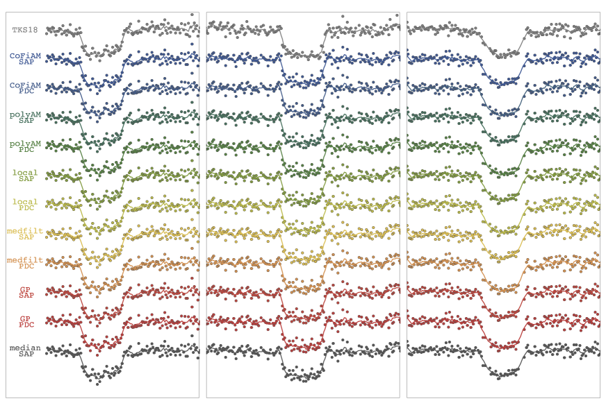
Figure 1: Method marginalized detrending. Comparison of five different detrending methods on two different data Kepler products. Top curve shows the Kepler reduction used in  (?) and the bottom curve shows the method marginalized product used in this work.

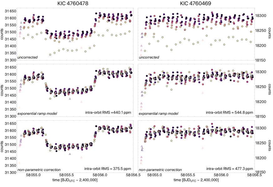
Figure 2: Hook corrections. (Top) The optimal aperture photometry of our target (left) and the best comparison star (right), where the hooks and visit-long trends are clearly present. Points are colored by their exposure number within each HST orbit (triangles represent outliers). (Middle) A hook-correction using the common exponential ramp model on both stars. (Bottom) The result from an alternative and novel hook-correction approach introduced in this work.

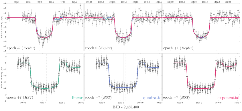
Figure 4: Moon solutions. The three transits in Kepler (top) and the October 2017 transit observed with HST (bottom) for the three trend model solutions. The three colored lines show the corresponding trend model solutions for model M, our favored transit model. The shape of the HST transit differs from that of the Kepler transits owing to limb darkening differences between the bandpasses.

Supplementary Materials

1 Materials and Methods

1.1 Kepler Re-analysis

1.1.1 Background

The original analysis of the candidate exomoon signal is described extensively in Section 8 of  (?). We refer readers to that work for the details of our original interpretation of the data. We briefly recap here the case for Kepler-1625b as a candidate exomoon host.

The analysis in  (?) was the largest and most ambitious search for exomoons to date, requiring many years to complete. Consequently, the data used in that study were first downloaded on November 10th 2014. Since the Kepler Science Processing Pipeline (see  (?)), built by the Kepler Science Operations Center (SOC), evolved over the years of the primary mission, the data analyzed in  (?) does not represent the most up-to-date data product at the time of writing. The three quarters in which Kepler-1625b is observed to transit are quarters 7, 13 and 16. In  (?), the simple aperture photometry (SAP) time series used were produced by SOC pipeline v9.0.3 (corresponding to data release DR21) for quarters 7 and 13 and v9.0.7 (DR22) for quarter 16. At the time of writing, the most up-to-date (and the final) data release is DR25, for which quarters 7, 13 and 16 were processed by SOC v9.3.24, v9.3.29 and v9.3.31.

Based on our prior experience with Kepler data products, we did not anticipate the Kepler photometry or case for the exomoon candidate would significantly change as a result of going from SOC v9.0 to v9.3. Nevertheless, in this more detailed and focused study, we decided to revisit the Kepler photometry and verify that this was true, as well as ensure that our results are robust against choice of detrending method.

Joint modeling of the original data had suggested the presence of a large moon in the system, with statistically significant drops in flux appearing on the wings of these transit events. Based on DR25 estimates of the star’s radius ($1.793\pm 0.263\,R_{\odot}$), the planet is approximately the size of Jupiter. Meanwhile the photodynamical fits to the data, which require a self-consistent moon model for all transit events, suggested the moon’s radius was comparable to that of Neptune (although with sizable uncertainty). No bad data flags (such as reaction wheel zero crossing events) or anomalous pixel behavior (such as that seen a previous candidate Kepler-90g;  (?)) could explain the candidate signal at the time, nor could we identify any astrophysical explanation besides the moon hypothesis that accorded well with the data in hand.

Despite this, we argued that three transits were insufficient to claim strong evidence for an exomoon detection, and so an additional validation observation was sought and awarded on the Hubble Space Telescope (HST). Twenty-six orbits amounting to ${\sim}$40 hours were awarded and the observations were executed on 28-29 October 2018.

In our analysis of the HST data, it was necessary to perform a joint fit with the Kepler photometry. To that end, we conducted a revised analysis of the Kepler data, now with the SOC v9.3 data product. Upon initial inspection of these results it was found that significant differences do exist between the revised Kepler data and the earlier release used for this target. In addition to the photometry, which has undergone noticeable modification, one changing value in particular – the crowding or blend factor (CROWDSAP), a measure of aperture contamination by nearby sources – appeared to play an important role in determining whether the moon model is favored. This is because blending can introduce transit depth variations which could be explained by a moon in proximity to the planet. Because this single value was such an important part of the moon fit we sought to determine the cause of this change from SOC v9.0 to SOC v9.3.

1.1.2 KIC 4760471 - The Phantom Star

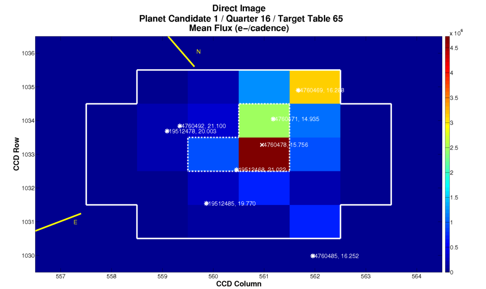
Figure S5: The “Phantom” Star. Model of the Kepler optimal aperture taken from the Data Validation Report (Q16 aperture), with the model star field overlaid. KIC 4760471 is clearly marked within the green pixel, but the star apparently does not exist.

In investigating the source of the modified crowding values we examined the Data Validation (DV) report for Kepler-1625b closely. This examination revealed that there is star included in the optimal aperture sky maps that does not exist. The source, KIC 4760471, is clearly present in the DV maps, situated almost directly between our target and the neighboring KIC 4760469, and in fact, the star is purportedly brighter than our target by about half a magnitude (see Figure S5). However, we find no evidence of this source in images from 2MASS, UKIRT, Pan-STARRS, Gaia, or our HST images. Nor is the star included in the catalogue of nearby sources available on the Kepler Exoplanet Follow-Up Observing Program (ExoFOP) website. We must conclude that this star is a spurious inclusion in the KIC, and this raises the question of how many other such stars there may be in the catalogue that may be producing erroneous contamination estimates. Indeed, this is not the first “phantom star” to be identified in the KIC;  (?) also reported the discovery of a spurious KIC inclusion that resulted a $\sim 50\%$ transit depth change for Kepler-445c.

After modeling what Kepler should be seeing based on the published Pixel Response Function  (?), we introduced KIC 4760471 into the model to test whether the star was actually included in the models for SOC v9.3 and earlier releases. We find that it cannot have been a part of the SOC model, despite its inclusion in the DV report, as the brightness and proximity of this phantom star would contaminate the optimal aperture by $\sim 50\%$ or more, and this is not reflected in the CROWDSAP numbers published by the SOC. This ultimately led us to conclude that the SOC v9.3 were accurate even if the DV report appears in error.

1.1.3 Method-Marginalized Detrending the Kepler Data

A critical aspect of light curve analysis is the removal of systematic trends in the data. For the exomoon search this is especially important, as we must be careful to neither produce nor remove the subtle signatures of the moon which, unlike planetary transits, will not show morphological repetition from one epoch to the next. Various approaches to detrending have been utilized in the literature, but no single method is considered the gold standard.

The Hunt for Exomoons with Kepler (HEK) project developed the Cosine Filtering with Autocorrelation Minimization (CoFiAM) method  (?), which was specifically designed for the moon search, as it focuses on preserving small / short duration features (possible exomoon transit signals) in the vicinity of the planetary transit. The algorithm represents the long-term trends as a sum of harmonic cosine functions with the longest period component being equal to the twice the baseline. The algorithm forbids components with periods (i.e. timescales) less than twice the transit duration, meaning that the Fourier decomposition of a transit is not disturbed by CoFiAM. This removes any long-term trends in the data, be they instrumental or astrophysical, while preserving short-duration events like those expected from an exomoon transit. We refer the reader to  (?) for a more in-depth discussion of the method.

In addition, it is worthwhile to explore other detrending approaches to see what effect they may have on the final results, precisely because the signal we seek is so subtle. To that end we examined the results from a number of fairly standard detrending approaches: a polynomial fit, a local line fit, a median filter, and a Gaussian process. The polynomial method is identical to CoFiAM except we replace the basis set from cosines to polynomials, exploring up to twentieth order and selecting the locally-minimized autocorrelation result. The local line fit is a polynomial fit up to twentieth order but only training on data immediately surrounding (we used $\pm 80$ hours) the transits and selecting the order which minimizes the Bayesian Information Criterion (BIC). The median filter uses a bandpass equal to five times the transit duration to remove long-term trends. The Gaussian Process regression adopts a square exponential kernel and trains on the entire quarter masking the transits.

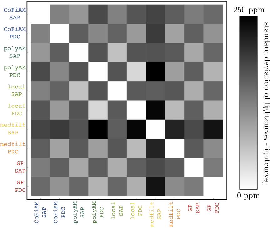
Figure S7: Kepler detrending comparison. Matrix plot of the standard deviations obtained when taking the differences between the resulting fluxes from each detrending approach. The plot is scaled such that white equals 0 ppm and black equals 250 ppm. For comparison the typical photon noise uncertainty in 600 ppm.

The regressed trend models for the SAP photometry are shown on Figure S6. We detrended both the SAP and PDC data with all five methods, giving a total of ten light curves as shown in Figure 1 of the main text. A visual examination of these results suggests no clear favorite or obviously problematic detrending, but we may compare residuals from the difference of two methods to gain a sense of where and to what extent they differ. A matrix representation of these residuals can be seen in Figure S7, where the maximum standard deviation peaks at $\sim 250$ ppm, much less than the formal photometric errors on the Kepler data of $\sim 590$ ppm. This suggests that the result is robust against choice of detrending method.

We decided to marginalize over the different detrendings to create a robust light curve to work with in what follows. To do this, we took the five SAP light curves and computed the median flux at each time stamp. The PDC data was not used here because the data have been corrected for contamination effects already and thus are expected to be slightly offset from the SAP results. The expectation then is that any anomalous features produced by one detrending method will be mitigated. The uncertainties on each data point are appropriately scaled up by quadrature addition of 1.4286 multiplied by the median deviation across the different methods at each time step (which had a median value of 34.6 ppm), thereby yielding uncertainties accounting for detrending differences. This effectively imposes a more stringent requirement for the moon to make its presence obvious in the data, since larger uncertainties provide more flexibility for the planet-only model. The final light curve is presented in Figure 1 in the main text.

1.1.4 Revised Photodynamical Fits of the Kepler-only Data

Although we have new HST data in hand, we decided to re-analyze the revised Kepler data in isolation before combining the data sets. The main purpose of this exercise was that later results can be placed in better context to assess which data set is primarily responsible for any interesting signals found. In  (?), Bayesian photodynamical fits were conducted on Kepler-1625b to test for the presence of a possible moon. This led to a Bayes factor between the planet+moon (M) and planet-only (P) model which would be classified as “very strong” evidence on the  (?) scale ($2\log K=20.4$). The third transit in particular seemed to dominate the signal and the strong dependency of our inference on just a single epoch led us to conclude that the case for an exomoon remained ambiguous despite the high Bayes factor (and ultimately led us to pursue follow-up observations).

Using the revised SOC v9.3 data, we performed the same fits for models M and P, as well as a transit timing variation model, T, and a zero-radius moon model, Z. The evidences, derived using MultiNest  (?), are presented in Table 2.

From this table, it is immediately apparent that the case for an exomoon is dramatically weakened using the revised Kepler data, going from $2\log K\simeq 20$ to $2\log K\simeq 1$. This naturally raises the question as to what exactly caused such a large decrease. In total, four aspects of the analysis have changed:

1. Revised analysis used a slightly contracted baseline

2. Revised analysis used method marginalized detrending, rather than just relying on CoFiAM

3. Revised analysis used updated and thus different crowding factors

4. Revised analysis used the SOC v9.3 data products, rather than the SOC v9.0

In principle, one or more of these must be responsible for the decrease in the evidence for the exomoon hypothesis and here we attempt to distill by elimination which one(s) it is.

The baseline (which is the temporal window around each transit used in the MultiNest fits) in our revised analysis was contracted from the original analysis. Because  (?) were blindly searching for moons in an ensemble out to 100 planetary radii from the host, transits were detrended with a baseline equal to an estimated 150 planetary radii. That calculation, detailed in  (?), was not only based on now out-dated system parameters, but also is excessive for the purpose of validating the exomoon candidate Kepler-1625b-i which has a hypothesized semi-major axis in the range of 20 planetary radii. We estimated that 80 hours on either side of the transit would easily accommodate the features of interest in our new analysis (whereas 98.8 hours was used in  (?)). Nevertheless, this difference could somehow explain the change and so we conducted a controlled experiment where we fit the exact original data from  (?), but contracted the baseline to $\pm 80$ hours. Rather than reducing the evidence, this actually boosted it slightly, with $2\log K$ increasing from 20.6 to 24.4 (here and in what follows we quote the Bayes factor between the M and P models only). This increase can be understood when considering the fact that a larger fraction of the data are affected by the moon-like signals. We also verified we recovered the same evidence as  (?) with all inputs left the same in two independent fits, which both gave the same result to within 0.6 in $2\log K$. These tests demonstrate that the contracted baseline is certainly not responsible for the decreased evidence, as we might reasonably expect.

Our second hypothesis was that it was the different detrending algorithms used that caused the difference. We therefore compared the fit that used the original data but truncated baseline (from the previous paragraph), with a fit that was identical except that the photometry was detrended using the method marginalized approach, rather than CoFiAM alone (but still using the SOC v9.0 data products and blend factors in both cases). This again only led to a higher evidence for the moon, with $2\log K$ now reaching 29.2. This therefore establishes that the decreased evidence for the moon model described at the beginning of this subsection, is not caused by either the baseline or detrending method used by  (?).

This leaves two remaining possibilities: the blending factors and/or the actual photometric data products. We took the method marginalized light curve produced from SOC v9.0 and fit it in two ways; one using the crowding factors produced by v9.0 and one using those from v9.3 - but everything else kept the same. The former of these two fits corresponds to the $2\log K=29.2$ case of the previous paragraph. The latter case gives a greatly reduced $2\log K=14.8$. Thus, the contamination factors must be, in part, responsible - likely as a result of transit depth variations.

The other possibility was investigated by repeating the previous experiment but instead comparing to a fit where the blend factors are those of v9.0 but the data input to the method marginalized detrending algorithm comes from the SAP light curve of v9.3. This causes the Bayes factor to decrease from $2\log K=29.2$ to $2\log K=6.8$, a decrease even greater than that due to blending.

We are therefore able to deduce that our revised analysis of the Kepler data alone leads to decreased evidence for an exomoon as a result of two changes introduced between SOC v9.3 and v9.0: i) the new blend factors and ii) the new SAP photometry. The choice of baseline and/or detrending method are certainly not responsible. Comparing the light curve from  (?) and/or the revised method marginalized version on the same v9.0 data products reveals that the largest difference, versus the v9.3 product, is the third transit in quarter 16. This transit appears distorted and asymmetrical in the original analysis, explained by a large moon carving out flux around the planetary transit. The new data shows a much cleaner signal more closely resembling the other two transits.

1.2 Hubble Observations

1.2.1 Observation Design

In a planet-moon transit event, an in-situ observer would see the moon either leading or trailing its host planet, and in rarer cases the event could begin with both bodies passing in front of the star simultaneously. To adequately observe an exomoon transit it is therefore imperative that observations begin well before the anticipated planetary ingress and conclude well after planetary egress, as we expect to see flux reductions due to the presence of a moon in these parts of the light curve. The separation in time between the planet and moon ingresses / egresses is directly connected to their sky-projected separation, which will be a function of the moon’s semi-major axis.

With a photodynamical moon model in hand from fits to the Kepler data it was possible to run the model forward in time to generate expected light curves for the October 2017 transit, though the morphology of the transit was poorly constrained when projected five epochs into the future. To determine the best start and end times for the HST observation we drew from the model posteriors and generated forward models based on these inputs, generating a range of possible outcomes. We set our start and end times such that exomoon ingress and egress features would be captured in the observing window to 95% confidence. We requested a start time as close as possible to Barycentric Julian Date (BJD_UTC) 2458054.8 and ending no earlier than BJD_UTC= 2458056.5.

For the observation we selected the G141 grism on Wide Field Camera 3 (WFC3), which is sensitive from $\sim$ 1.1 to 1.7 microns. This choice was motivated in part by the expectation that stellar variability, to the extent it is present, should be suppressed towards the infrared. In addition, because the observation would amount to some 40 hours on target, we knew that HST would pass through the South Atlantic Anomaly (SAA) for a significant fraction of this time, and WFC3 is one of the few instruments aboard HST that may be used during passage through the SAA. The grism creates a dispersion spectrum such that the light from each source is spread across the CCD, providing spectral information on the target and its neighbors. Use of the grism also allows for longer exposures, as it takes much longer for a bright target to saturate. It is worth pointing out that time on target is of paramount interest in carrying out such an observation; we wish to minimize telescope overheads, which can include data readouts that interrupt the observation, and the RMS of the observation is directly tied to the time on target.

The drawback to using the grism is primarily the fact that a suitable roll angle for the telescope must be selected, one that minimizes overlap between the target spectrum and neighboring spectra. With each spectrum illuminating roughly 135 pixels in the direction of dispersion and several pixels on either side of the spectrum’s central line, crowded fields must be modeled with care. Depending on the time of observation and the orientation of HST with respect to the Sun at that time, suitable roll angles may not be available. For the field containing Kepler-1625 we found only $\sim$ 20 of 360 degrees suitable for a grism observation.

We used the HST Exposure Time Calculator to plan the observations (ETC ID WFC3IR.sp.912655). Inputs were 1) the star’s J-band magnitude (14.364$\pm$0.029) from 2MASS; 2) $E(B-V)$ = 0.19, taking line of sight extinction $A_{V}$ to target = 0.594 (NED value taken from  (?), and assuming $R_{V}=3.1$; 3) a built-in Pickles model spectrum for a G0III star with $T_{eff}$ = 5610 K (the closest match available to Kepler-1625); and 4) zodiacal light, Earth shine and air glow models for the date of observation, also built-in options in the ETC. We found that a 300 second exposure would fall well short of the time to saturation, which the ETC calculated to be 508.74 seconds. We opted not to utilize HST’s spatial scanning mode, which moves the spacecraft perpendicular to the direction of spectral dispersion during each exposure, thereby spreading the light onto more pixels. Spatial scanning was inappropriate for our observation, both because we were not close to reaching saturation (typically the primary motivation for spatial scans), and because the crowded field meant the spatial scan would have to be extremely short, and potentially unachievable by the spacecraft given the length of each exposure. We note also that the software provided by STScI for reduction of the HST data does not currently support spatial scanning mode.

The standard data reduction pipeline distributed through STScI, aXe  (?) requires at least one direct image of the target (i.e. without the grism) so that spectral calibrations can be made. Using source locations derived from the direct image using SourceExtractor  (?), the aXe software is designed to calculate the position of each spectrum, the wavelength solution for each pixel, and contamination from nearby sources. A single direct image using the F130N filter was made at the start of the observing run with an exposure time of 103.129 seconds, followed by a total of 232 grism exposures. All data were taken in the 256$\times$256 subarray to reduce overheads. Each grism exposure lasted 290.776 seconds, well short of the saturation time. SAMP-SEQ was set at SPARS25 and NSAMP was 14, meaning there were 14 non-destructive readouts of each exposure at roughly 25 second intervals. These multiple readouts are useful in part for rejecting cosmic rays within the front-end data processing pipeline calwf3.

Roughly 3100 seconds, or 51.67 minutes, were available for observing the target during each orbit. The remaining time in each orbit (about 44 minutes) were unusable as the target was occulted by the Earth. For all but two orbits, there were only 72 seconds of unused visibility time. For the first orbit 130 seconds went unused, and for the 15^th orbit, 270 seconds went unused. This was due to increased overheads, namely a full guide star acquisition, which takes longer than re-acquisition and reduces the number of exposures that can be made in an orbit. Each exposure was long enough that data dumps could be made in parallel; therefore, there were no gaps between the first and last exposure in a given orbit.

It was found that only three of our exposures would occur during passage through the SAA, which was fortuitous. For most of the observation SAA passage was restricted to times when the target was occulted by the Earth, when no data could be taken. For these SAA-affected exposures the Fine Guidance System (FGS) cannot be used; instead, HST must use gyro control to stay on target. The gyros are known to have a pointing drift on the order of 1.5 mas per second, meaning that for our ${\sim}$290 second exposure we could expect the target to drift by approximately half an arcsecond.

1.2.2 Execution

Observations began at 6:52:15 (UTC) on 28th October 2017 and ended at 23:20:08 on 29th October 2017. No malfunctions of the spacecraft were detected. Three of the 232 exposures were indeed affected by passage through the SAA, in line with expectations. While the SAA had no discernible effect on the photometry itself, pointing drifted considerably during these exposures, as expected. The spectra from these images, landing on neighboring pixels and significantly dilluted by smearing, showed significantly different flux levels, even with appropriate pixel sensitivity corrections, and were therefore left out of our final analysis.

The final orientation of the spacecraft (provided in the header as the position angle of HST’s V3 axis) was $\sim 249$ East of North and produced a clean spectrum of the target with minimal contamination from nearby stars.

1.2.3 Data Preparation

For initial processing of the raw data files from STScI we followed the WFC3 IR Data Reduction Cookbook, using updated configuration and reference files where available, and making minor updates to source code when deprecated packages were still in use and caused fatal errors. We refer interested readers to the Cookbook for details on the data reduction. We utilize the .flt files produced by the front-end calwf3 pipeline, which account for a number of known systematics and perform cosmic-ray rejection. We point out that while the calwf3 performs a flat field correction, for grism observations the flat field division is unity everywhere, as the flat fielding for grism images is intended to be performed later as a part of the spectral extraction process.

The standard aXe software is unable to handle images taken in subarray mode, so each $256\times 256$ image must be embedded in a larger $1014\times 1014$ array before processing. It is important that the images be embedded in the correct position, as subsequent flat fielding and background removal are performed on a pixel-by-pixel basis. We modeled our own embedding code after a python script provided by STScI, which we were unable to run on our machines. We verified the embedding was done correctly by eye, matching obvious artifacts in the master sky image and the flat field cube to the same artifacts that are readily apparent in the images pre-correction. With this step completed we could follow the instructions of the cookbook.

Unfortunately we were unable to follow the prescribed reduction beyond the axeprep stage of the cookbook, as we experienced a persistent breakdown with the axecore task which we were never able to resolve. The axecore tool is responsible for automated spectral extraction. From here on we wrote our own code to analyze the data.

Following the STScI prescription, the background flux levels are calculated by finding the median flux of the image, masking out pixels with greater than 5 electron counts. The Master Sky Image  (?), calculated from in-orbit observations, is then scaled up by the median background flux level at each time-step and subtracted. This step removes the well-documented “breathing” effect that appears in HST time-series observations, which has been attributed to thermal fluctuations in the telescope as it orbits the Earth. An additional flat-fielding must then be performed, using the flat field data cube produced from pre-flight laboratory testing. The flat field cube encodes four polynomial coefficients at each pixel location to model the pixel sensitivity as a function of wavelength.

The axecore task is designed to calculate a wavelength solution for each pixel in the spectrum, and with this information a wavelength-specific flat-fielding can be performed. However, due to the code breakdown we did not have wavelength solutions in hand until later in the analysis. While the pixels show significant sensitivity variation across the CCD, we found there was minimal variation across the wavelength range for any given pixel (typically less than 1%), so we opted to compute the median sensitivity for each pixel and we used these values to perform the flat-fielding. We are thus marginalizing over intra-pixel sensitivity variations, but we point out that STScI documentation also suggests G141 grism observations may be flat-fielded using the F140W flat field which also does not encode intra-pixel sensitivity variations. We compared our median G141 flat field image to the F140W flat and determined that flattening the G141 cube was a more faithful rendering of the wavelength-sensitivity information for the grism.

1.2.4 Imputation of Bad Pixels

Following the flat field corrections there remained $\mathcal{O}(10^{3})$ pixels that were clearly outliers, as evident from a median stack of the images. Wherever possible, we elected to perform imputation of all time stamps associated with these outlier pixels. The tasks of outlier identification and imputation are treated independently.

To identify the outliers we start by calculating median pixel values across our observations, which should reveal pixels that behave anomalously in more than 50% of the exposures. This superstack is done on all images grism images, except for numerous images which were identified during preliminary analyses as behaving in a non-representative way: namely cadences 107, 116, 125 and 126; as well as orbits 1 (telescope settling), 7 (transit ingress) and 18 (transit egress). Each superstack pixel has an uncertainty equal to 1.4286 multiplied by the median absolute deviation (MAD) across all times.

Since the grism spreads the target spectrum along the pixel rows, we expect (and indeed observe) that the observed flux follows a smoother pattern along the rows than the columns. Exploiting this fact, we extract each row’s flux vs column index from the superstacked image and look for outliers along each row independently.

We do this by constructing a 3-point moving median and then training a Gaussian process (GP) with a squared exponential kernel on the result. This GP is then evaluated on all column indices, computing residuals as we move along. A median-version of the reduced $\chi^{2}$ is computed to re-scale. We define residuals as the difference from the GP normalized by the pixel’s uncertainty. We also scale the uncertainties such that the median version of the residual’s reduced $\chi^{2}$ equals unity. Outlier pixels are then flagged as those which depart more than 10 $\sigma$ (chosen after some experimentation) away from the GP model. Note that our GP lacks predictive power on the edge columns and this process does not consider column pixels during the search.

In addition to this procedure, we flag pixels as an outlier if the pixel’s derived uncertainty across all images exceeds 20 $\sigma$ of the median error of the row’s pixels, where $\sigma$ is again coming from another MAD.

If a pixel is flagged as an outlier but has an immediate neighbor of similar flux, we remove the outlier flag. This is done by first computing the maximum deviation of each superstacked pixel with its row-wise precursor and successor and then seeing if the candidate outlier is less than 10 $\sigma$ away from the median deviations seen in that row (where again $\sigma$ comes from the MAD). This was necessary to avoid killing zeroth-order spectrum features which look like islands of outliers in a single row (though we do not attempt to use zeroth-order features for analysis, as the target’s zeroth-order is off the CCD).

Imputation is not performed using medians as this essentially represents a zeroth order polynomial which is not sufficient to capture the gradients observed across the pixels. Instead, for each pixel in the image we produce a predicted flux based on a 1-dimensional spline interpolation with two pixels preceding and two pixels following it in the row. We found that a 1-D row interpolation is superior to a 2-D interpolation, as the latter does not adequately handle pixel replacement across the spectrum peaks, that is, perpendicular to the direction of dispersion. If the pixel has been flagged as an outlier it will be replaced with the predicted flux. An exception to this rule is if one of these four training pixels is itself an outlier. In such cases, we flag the pixel as an irreplaceable outlier.

After the first round of outlier identification and imputation, we ran the algorithm a second time. This process led to the identification of 1756 outlier pixels, of which 634 were irreplaceable whose fluxes were simply set to NaN after this point to mask them.

Finally, we note that the spectra produced by the grism are inclined 0.5 degrees with respect to the pixel grid, per WFC3 Grism documentation. We therefore use a standard SciPy package  (?) to rotate the image clockwise by 0.5 degrees, performing a 3rd-order spline interpolation, thereby aligning the spectra with the $x$-axis. This simplifies the extraction of the spectra considerably, as the optimal aperture may be neatly aligned with the image grid, and produces no discernible artifacts in the spectra. The pixel errors must also be rotated, which is potentially problematic if the errors across the image were random. However, since the errors scale predictably with flux levels this rotation is also well behaved, and the resulting distribution of errors across the image is unchanged from the native images.

1.2.5 Optimal Aperture

The target’s point spread function is centered in the rotated images at approximately $x=515$ and $y=531$ (where $x$ represents the column index and $y$ the row index). To extract photometric time series, we elected to employ simple aperture photometry rather than modeling the complex point spread function (PSF) observed. This is well justified since the high angular resolution of HST, combined with our observational design, means that we do not see significant overlap of neighboring sources with the target.

In choosing an aperture, we could simply draw a broad box around the target by hand, but instead we elected to choose an optimal aperture which minimizes the scatter in the final target light curve. The optimal aperture was found in a two-step process. First, we setup a grid of 105,840 candidate apertures where each permutation has a unique aperture defined by four parameters, $\{x_{\mathrm{min}},x_{\mathrm{max}},y_{\mathrm{min}},y_{\mathrm{max}}\}$, such that the aperture is bounded by $x_{\mathrm{min}}\leq x\leq x_{\mathrm{max}}$ and $y_{\mathrm{min}}\leq y\leq y_{\mathrm{max}}$. The grid of candidates spans the range $426\leq x_{\mathrm{min}}\leq 480$, $481\leq x_{\mathrm{min}}\leq 599$, $515\leq x_{\mathrm{min}}\leq 530$ and $532\leq x_{\mathrm{min}}\leq 544$, where we step between the extrema in 2-pixel intervals. We remind the reader that these pixel values do not correspond to the native images from HST, but to our rotated image, for which there is an offset. In each of these candidate apertures, we extract a white light curve for the target and correct for the hook effect using a simple exponential ramp (explained in detail in Section 1.2.6). While we eventually developed our own approach to removing the hook trends, this simple model does reasonably well correcting for charge trapping, and thus observations are expected to be stable within each orbit, although visit-long trends have not been corrected for at this point.

As visit-long trends persist, and there are of course flux decreases caused by Kepler-1625b’s transit, as well, comparing the raw root-mean-square (RMS) of each candidate aperture’s is not an appropriate cost function to score the different apertures. Instead, we reasoned that if we mask the times during the ingress and egress of the planetary transit (which take up one HST orbit each; orbits 7 and 18 respectively), then we should expect the photometry to be stable within each orbit (but not necessarily between each orbit). We further mask the first orbit, which appears to represent a settling-orbit for the photometric behavior and is typically discarded in similar studies. Finally, we also mask time stamps 107, 116, 125 and 126 where we later came to suspect outlier behavior. The remaining 202 points (of the original 232) are then grouped into their respective orbits and the RMS of each is computed. We then define a cost function as the mean of these RMS values (23 in total).

This process identified an optimal aperture defined by $456\leq x\leq 581$ and $526\leq y\leq 542$. However, the grid search used a resolution of 2-pixels in its search and further more used a fast but sub-optimal hook correction method. As described in Section 1.2.6, we found a novel non-parametric hook correction method is able to out-perform the exponential model and better capture the sharp hook morphology. We therefore performed a second-stage in our search where we essentially walk the aperture in 1-pixel intervals away from the previously found solution. Each bound (i.e. $x_{\mathrm{min}}$, $x_{\mathrm{max}}$, $y_{\mathrm{min}}$, $y_{\mathrm{max}}$) is perturbed by $\pm 1$ pixel to create 8 candidate grids, as well as the original solution to give a ninth. Across these 9 possibilities, we extract photometry as before but this time perform the more computationally intensive non-parametric hook correction described in Section 1.2.6. If a better aperture is found amongst the 9 options, we walk to that solution and repeat, else we stop.

In practice, we perturbed the optimal aperture from stage one adding a random integer between -2 and +2 to each bound and walked from that position, in order to test if the walker would return to the same solution. Indeed this is what happened and the final optimal aperture returned to $456\leq x\leq 581$ and $526\leq y\leq 542$, which has mean intra-orbit RMS of 375.5 ppm. In what follows, we set value that value, 375.5 ppm, as the standard photometric error for this optimal time series.

1.2.6 Modeling the Hooks

A well-known feature of time-series observations on HST are the exponential ramps or hooks, e.g.  (?, ?); a phenomenon that’s also been observed in Spitzer data, e.g.  (?, ?, ?, ?). As the observation begins, the flux readings ramp up with each subsequent exposure towards a saturation asymptote. This is thought to be due to charge trapping in the CCD  (?). Once the observations are interrupted, either due to occultation of the target by the Earth or through a non-parallel data dump, the ramps resume.

Common previous approaches for removing this systematic include templating the ramps from the out-of-transit orbits to detrend them in all other orbits  (?), and assuming a parametric model fit (typically using exponential functions) to each ramp for removal  (?). The templating approach is not ideal for our observations since we do not know which orbits are in- or out-of-transit a priori, due to the candidate exomoon. For this reason we initially pursued an exponential ramp model. The results from this approach were certainly reasonable and provided a clear transit recovery. Despite this, in our quest to extract as much information as possible from these observations, we devised an alternative strategy that ultimately provided a superior correction.

The inspiration behind our new approach can be seen in Figure 2 of the main text. Each orbit is typically comprised of 9 exposures, which are shown with distinct colors in the figure, and can be labelled with the index $v=1,2,...,9$. If one considers just the $v=1$ points, the light curve appears remarkably clean, and the same argument holds true for any specific choice of $v$. This is understandable if we consider the fact that each observation $v$ shares a common observational history; that is, the $v=1$ exposures all occur immediately following target acquisition after occultation, the $v=2$ exposures all have a common history following $v=1$ observations, with all the charge trapping associated with those exposures, and so on. These common histories will then act as a baseline flux level for each $v$ that may be independently corrected. We therefore hypothesized that these nine light curves could be combined by simply scaling them independently to create one coherent light curve. We assign 9 scaling factors, $\gamma_{v}$, to each and treat these as unknown parameters to be solved for.

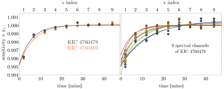
Figure S9: HST hook model comparison. Left: Comparison of the two models for the WFC3 hook; an exponential ramp fit (solid) and a novel discrete model introduced in this work (points). The left panel shows the results from the white light curve of the target and a comparison star. Right: Same as left except we show the 9 different spectral elements used in this work for the target. The v index is the exposure number within a given orbit.

Following our earlier argument in Section 1.2.5, we expect the hook-corrected light curve to exhibit stable intra-orbit photometry (but not inter-orbit). We therefore use the same cost function as used earlier, namely the mean intra-orbit RMS. We iteratively optimize for the $\gamma_{v}$ terms until the cost function improves negligibly. The final $\gamma_{v}$ terms are shown in Figure S9, where we also overplot the optimized exponential ramp model for comparison. This plot reveals that the exponential ramp model is not able to fully capture the very sharp turn-on of the hook. The exponential hook correction light curve is also shown in Figure 2 of the main text, where the mean intra-orbit RMS is considerably higher at 440.1 ppm (versus 375.5 ppm). Nevertheless, an exomoon-like decrease in brightness is observed in both versions following the planetary transit.

We highlight that our non-parametric approach is somewhat guaranteed to out-perform the ramp model due to more degrees of freedom. However, the ability to capture sharper hooks, combined with the more agnostic nature of the method’s assumptions ultimately led to us to use this method for our final hook-correction. We highlight that 375.5 ppm per 300 seconds corresponds to 154.8 ppm per Kepler long-cadence, which is 3.8 times lower than the median Kepler uncertainty resulting from our method marginalized detrending (589.9 ppm). Thus, HST greatly out-performs Kepler on this target. For this reason, one might reasonably expect that the HST data will be the dominant transit epoch for constraining putative moons.

From Figure 2 in the main text, an apparent decrease in brightness is evident with both versions of the hook correction for Kepler-1625, occurring a few hours after the primary transit has finished. The precise shape of this moon-like dip appears dependent upon the trend assumed in the data, which is discussed in detail in the main text.

1.2.7 Wavelength Solution

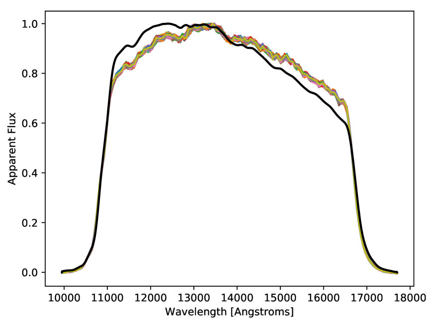
Figure S13: Wavelength solution. Calculated blackbody for Kepler-1625 multiplied by the G141 response function (black). The spectrum of Kepler1625 extracted from each HST image is overlaid in multiple colors (for each exposure). Both curves are normalized by dividing out their maximum values. Note the overprediction of the model at shorter wavelengths and underprediction at longer wavelengths.

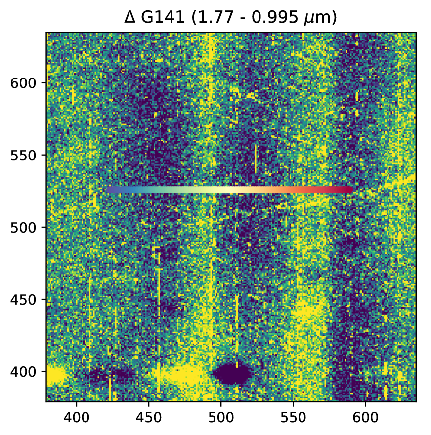
Figure S14: Wavelength-dependent pixel sensitivity. Change in pixel sensitivity across the G141 wavelength range. The color range is $\pm$ 1%. Towards the purple end short wavelengths are more sensitive than longer wavelengths, while at the yellow end longer wavelengths are more sensitive. The full width of the target spectrum’s response function is overplotted.

To derive a wavelength solution for each pixel we extracted the spectra for the target and comparison star and found the best fits (minimizing $\chi^{2})$ to a model spectral profile (Figure S13). The model is produced by multiplying the G141 response function by a blackbody curve, the latter produced using published values for the stars’ effective temperatures. By examining the wings of the model curve (where sensitivity falls off rapidly) and comparing to the extracted spectra the fits are excellent. We note however that this simple model overpredicts the flux at shorter wavelengths and underpredicts at longer wavelengths, as can be seen in Figure S13. We examined whether this discrepancy could be due to our marginalizing over the wavelength information in the flat field, as there is a distinctive wave-like structure in the pixel sensitivities that propagates across the CCD in the direction of dispersion. In some places on the CCD shorter wavelengths are more sensitive than longer wavelengths, where in other places the reverse is true (see Figure S14). As we marginalize over the wavelength information in the flat field, this information is lost.

However, we find that this intra-pixel flat-field structure cannot explain the spectrum-model discrepancy in Figure S13, as flux errors across the spectrum average out to be less than 0.2% for any flux bin when accounting for the wavelength dependence, whereas the discrepancies are clearly well in excess of that. We speculate that the discrepancy merely arises from the fact that stars are not perfect blackbodies. In any case, these discrepancies do not invalidate the wavelength solution, as the rapid fall-off in sensitivity at either side of the spectrum clearly matches the sensitivity curve very well.

1.2.8 Nearby Uncatalogued Source

Upon inspection of the HST images it became clear that a previously uncatalogued point source is present in close proximity to the target. The object shows up in every image obtained by HST and cannot be an artifact on the CCD, as it moves like all the other point sources during the three SAA-affected exposures. By every indication it is a another spectrum for a nearby point source.

To estimate its position on the sky we simply take the first pixel along the spectrum for which Flux $>$ 0. Note that this is not the sky position of the star. However, we may do the same for the target star and nearby KIC 4760469, for which the sky separation and position angle is known, and thereby orient ourselves to calculate the sky separation and position angle of the uncatalogued source.

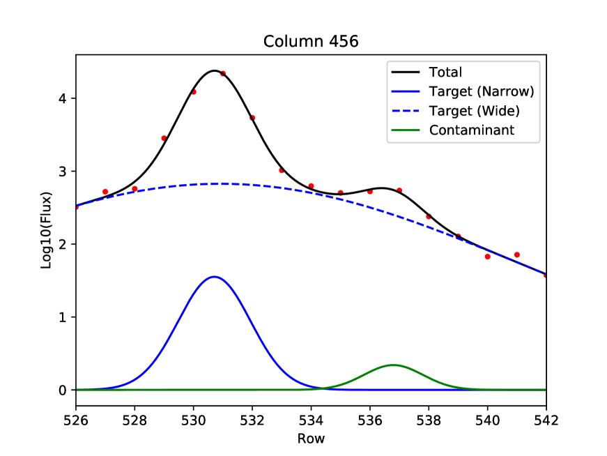
Figure S15: Modeling the uncatalogued source contamination. A single column within the HST optimal aperture, fitting three Gaussians to the source and the contaminating uncatalogued source. Pixel fluxes are shown by the red data points. The blending is calculated by taking the inverse of the starlight fraction within the optimal aperture originating from the target star.

To calculate the magnitude of the new source, we step through each column along the spectra and fit a three-Gaussian model to the data. One Gaussian is fit to the new (contaminating) source while two Gaussians are fit to the target – one narrow, and another wide. The combination of these two Gaussians do an excellent job fitting the peaky-but-broad profile of the target star, with the wider component accounting for what appears to be flux bleeding into neighboring pixels (see Figure S15). Having stepped through every column, the areas under these three Gaussians can be computed, and the flux of the uncatalogued source may be compared to that of the target. With this information the relative magnitude with respect to the target may be computed.

We find that the star is located $\sim$ 1.78^′′ away from the target at Position Angle 8.5 degrees East of North. We compute a Kepler bandpass magnitude of 22.7. To compute a blend factor we take the same approach as before, i.e. modeling the target and the contaminant with three Gaussians, only now we restrict the window to the optimal aperture see Figure S15. We compute a blend factor of 1.000328, indicating an extremely small contribution from the uncatalogued source on our light curve. Furthermore, an extracted light curve from the uncatalogued source shows a variability of 0.33%, so its contribution to the target light curve is 1 ppm. We therefore ignore it in subsequent analysis.

Using a Gaia-derived distance of $(2460\pm 220)$ pc to the target, we may calculate the physical separation of this uncatalogued source from Kepler-1625, under the assumption that the two objects are at the same distance. We find that separation would be ${\sim}$4400 AU, placing it well within the gravitational influence of Kepler-1625. It is however impossible with the data in hand to determine whether these objects are in fact physically associated.

1.2.9 Visit-long trends

In addition to the breathing and hook effects, one other well-known source of systematic error requires correction - the visit long trend  (?). Visit-long trends with WFC3 are typically modeled as a linear slope (e.g. see  (?, ?, ?)). However, our observations are unusual in that they span 40 hours, far more than the few hours used when observing transiting planet on short orbital periods. These trends have not yet been correlated to any physical parameter related to the WFC3 observations  (?), and indeed not all observations appear affected. Simple inspection of our white light curve, using either the exponential or non-parametric hook correction, show clear evidence for a visit-long trend (see Figure 2 in the main text).

Although a linear trend is the most common approach (e.g. see  (?, ?, ?)), we note that  (?, ?) report improved fits using a quadratic model and so we considered both models in this work. We further extended our investigation to include an observation-long exponential ramp model. This last model is motivated by visual inspection of the light curve, which appears to ramp up and flatten, as well as the asymptotic behavior it introduces which is more physically motivated than an ever-increasing/decreasing trend. We speculate that it could perhaps be caused by the same charge trapping that causes orbit-long ramps, only operating on a much longer timescale.

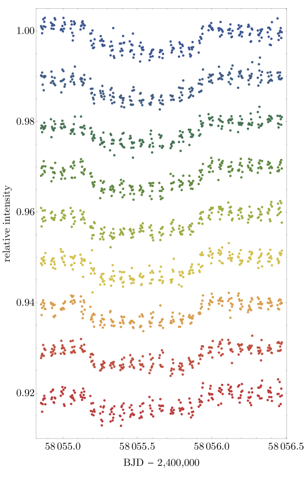
Figure S11: Spectral analysis. Nine spectral channels, color-coded in wavelength from the bluest channel (top) to the reddest (bottom), extracted from our WFC3 photometry of Kepler-1625b. Naturally the noise in each channel is considerably higher than the white light curve.

If we look at specific spectral channels, rather than the white light curve, a flux offset occurs between the 14^th and 15^th orbits for the reddest wavelengths (see Figure S11). This moment in time corresponds to the HST visit change, during which the spacecraft performed a full guide star acquisition at the beginning of the 15^th orbit, which placed the target spectrum $\simeq$0.1 pixels away from where it appeared during the first 14 orbits. This discontinuity appears in the raw photometry mid-planetary transit and is potentially problematic due to the fact that it can mimic a moon signal. Any model placing the moon at the kink would be immediately suspect.

In the white light curve, a flux offset at this time is barely noticeable but since the red spectral channels contribute to the white, then we deemed it necessary to allow for an offset term in our three trend models.

Since only centroid position changes during the visit switch, whether the visit-long trend be astrophysical or due a long-term instrumental effect, there is no reason to expect a different functional form or function parameters to become introduced at the instant of the visit change. For this reason, we generally expect a smooth continuous function (such as the linear, quadratic or exponential models) but with an offset term to account for any remaining pixel sensitivity variations. We therefore did not consider models described by two completely independent polynomials, for example, on either side of the visit change.

Since the visit-long trend occurs on a long timescale, it is inextricably mixed with the transits of the planet and possible moon. In such a case, strong covariances are expected between the trend parameters and the transit parameters and thus joint fitting is required. Our joint fits are described later in Section 1.3, but for now we point out that all six visit-long trend models were regressed in conjunction with the transit models considered (e.g. models M, P, T and Z), but independent of one another. In this way, we can rank the different approaches based on their Bayesian evidences, as well as the resulting associated physical parameters.

The results of these fits using the planet+moon (M) transit model may be seen in Figure 4 of the main text, with Bayesian evidences tabulated in Table 1 in the main text. All of the fits are able to explain the previously noted decrease in brightness towards the end of the observations as being due to a moon transit, although the duration and depth of the event vary somewhat between the three trend models. In the exponential trend model the moon fully egresses before the end of the observation, while in the linear and quadratic fits the moon is still in the process of transiting. However, in virtually every case the dip remains discernible after detrending has been performed. Note that all of these models were found to be preferable to any other transit model (e.g. T, Z or P) attempted using the Bayes factor (we direct the reader to Section 1.3 for a more detailed discussion of model comparison).

1.2.10 Is the moon-like dip instrumental or astrophysical?

As noted earlier, there appears to be a decrease in flux in our WFC3 photometry towards the end of our observations. Since we are primarily interested in the possible existence of exomoons in this work, that decrease is of particular importance as it will greatly affect photodynamical model fits, if real.

To assess whether this dip is instrumental or astrophysical in nature, we considered three tests: i) inspection of the comparison star ii) inspection of the centroids iii) a chromatic test. The chromatic test is described later in Section 1.3.11, but we here describe i) and ii) in more detail than possible in the main text.

The only other bright star with a full spectrum in the HST images is KIC 4760469. This star was not observed by Kepler, but is listed as a $0.84$ $R_{\odot}$ $5555$ K main sequence star in the KIC. Accordingly, it is expected to be photometrically stable and provide a good test for our correction algorithm. We therefore applied the exact same routines to this star as was done for Kepler-1625.

As seen in Figure 2 in the main text, the comparison star displays no obvious long-term trends that might be attributed to instrumental systematics, apart from a gentle upward slope at the beginning of the observation which is also seen in the light curve for Kepler-1625b and is cleanly corrected with our detrending. We used MultiNest to compare the linear, quadratic and exponential trend models and found all three were similar in evidence, with the quadratic model being slightly favored.

In terms of assessing if the moon-like dip associated with Kepler-1625b is real or not, the relevant region is visible from BJD 2,458,456 of Figure 2 of the main text. The photometry appears quite stable at this time and certainly no indications of an instrument-induced flux change.

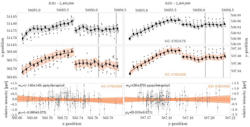
Figure S10: HST centroids. Top row shows the centroid position of our target in both row (left) and column (right) pixel index, with a GP model overlaid (shaded region). Middle row shows that the same but for our best comparison star (right). The column positions have been offset by 0.1 pixels after the visit change to more easily fit them on a single scale. The vertical grid lines mark the location of the moon-like dip seen in the photometry of the target, where we note that no peculiar behavior is evident. The lowest row shows a correlation plot of intensity versus centroid position for the comparison star (second visit), where no clear dependency is evident either.

The second check we performed was to look at the centroids. Column ($x$) and row ($y$) centroids were computed from the optimal apertures of the target and comparison star and are shown in Figure S10. We highlight that the $y$ position has been decreased by 0.1 pixels after the visit change (for both sources) to fit them on the same scale, but the $x$ position has not been altered. Both the target and the comparison star show nearly identical centroid behavior, as expected.

The moon-like dip occurs across several orbits and thus the only way centroid variations could explain the dip would be an inter-orbit centroid variation. We therefore take the median centroid position of each orbit as binned points, shown by the black data in Figure S10. Aside from the visit change shift, there are no substantial changes in the inter-orbit centroid position, and certainly not around the time of interest (highlighted by the vertical lines).

Comparing the centroids to the flux variations observed can also be used to gauge how feasible it is that the moon-like is a product of these clearly small centroid changes. From our later fits of the target, we find that the visit-change flux offset is $(330\pm 120)$ ppm, $(180\pm 190)$ ppm and $(220\pm 140)$ ppm for the linear, quadratic and exponential models respectively. That corresponds to a decipixel (0.1 pixels) change in the $y$-position and about half that in the $x$ direction. Together then, this indicates that a decipixel shift in centroid position may slightly affect the photometry at the $\sim 200$ ppm level.

Inspection of the centroid variations after the visit-change - where the moon-like dip occurs - reveals a shift of approximately one-tenth of a decipixel (see Figure S10). Since a one decipixel shift is associated with a 200 ppm photometric change, we argue that it is highly unlikely that $\sim$500 ppm moon-like dip is a product of centroid shifts. However, we highlight that a quantative calculation of the centroid-induced photometric change in this region is not possible without knowledge of the functional form governing the residual inter-pixel sensitivity.

The above considered the centroid-flux correlation as observed using just the target, but the comparison star is also worth considering. If we assume the comparison star is stable, a flux versus centroid plot reveals much more information than that from above. However, we caution that such a plot only maps the sensitivity at this part of the detector and this may not necessarily be the same as that on the target itself. Taking the second visit data only, which is the region of interest, we computed a cross-correlation of normalized intensity versus $x$ and $y$ centroid positions, as shown in Figure S10.

No clear relationship is apparent from inspection of this plot. If there is a functional relationship between flux and pixel position, it appears to operate at a level below the noise of this data. Certainly no linear relationship is detected, with the Pearson’s correlation coefficient being consistent with zero for both $x$ and $y$ positions. Computing a linear slope in both cases implies that flux depends on $x$ and $y$ centroid position as $(-140\pm 180)$ ppm/decipixel and $(+50\pm 480)$ ppm/decipixel respectively. These numbers are consistent with the $200$ ppm change observed in the target for a decipixel shift during the visit change, despite being located at a different part of the detector.

We can make some simplifying assumptions in order to have an approximate estimate of the centroid-induced flux changes expected around the moon-like event. These assumptions should not be treated as truth, but rather as plausible and necessary for quantitative progess. Although we don’t know the true functional form, let’s assume that intensity indeed maps linearly with centroid position for small changes (exploiting a Taylor expansion logic). We further assume that the detector’s behavior on the comparison star is representative of the source. The $x$ range in the source’s second visit is 0.25 decipixels, which would be associated with a $<50$ ppm change using the assumptions above. Similarly, the $y$ range is 0.1 decipixels, implying a maximum variation of $<50$ ppm. Accordingly, although this is certainly a simplified model, it suggests a 500 ppm flux change is quite unlikely to arise from the centroid variations.

1.2.11 Spectral analysis

With a low-resolution transmission spectrum we may also attempt to characterize the planet’s atmosphere. A transmission spectrum, measured as the changing transit depth as a function of wavelength, can potentially reveal molecular absorption features in the atmosphere, and with sufficient sensitivity it may also be used to infer the planet’s mass, as atmospheric abundances and Rayleigh scattering will be sensitive to the planet’s surface gravity.

We split our optimal aperture in 10 even segments along the column direction and corrected for the hook independently in each using our non-parametric algorithm. We found that the tenth and reddest channel was quite unstable and thus neglect it in what follows. Light curves from the other nine channels are shown in Figure S11, and final transmission spectrum is shown in Figure S12.

We utilized our own MCMC code to explore parameter space and generate a best-fit transmission spectrum using the Exo-Transmit code  (?, ?, ?, ?). The generated high-resolution spectrum is binned at the appropriate wavelengths to test against the data, which also includes the Kepler transit depth, for a total of 10 data points across the wavelength range, 9 of which are derived from the WFC3 spectrum.

The variable inputs are radius of the planet $R_{P}$, surface gravity of the planet $g_{P}$, and (optionally) a cloud deck atmospheric pressure. The code treats the atmosphere as opaque at pressures higher than the cloud deck pressure value, corresponding to greater depths and effectively increasing the radius of the planet. All variables have uniform priors. Three other inputs (stellar radius, temperature, and metallicity) are fixed, as discussed below.

$R_{P}$ was allowed to range from half to twice the radius of our best fit planet radius, while $g_{P}$ is restricted between 1 and 1000 m s^-1. The mass may then be inferred from the combination of surface gravity and planetary radius. The cloud top pressures (when applied) could range from 1 to $10^{7}$ Pa, allowing for virtually no cloud deck down to $\sim$ 100 atmospheres. To speed up convergence the MCMC was initialized with reasonable first guesses for the radius (from the transit depth) and surface gravity of the planet (randomly chosen to be some value less than 30 m s^-1.

We fix the stellar radius at 1.793 $R_{\odot}$, as there is nothing in the transmission spectrum that can constraint the size of both the planet and the star. In addition, we fix the metallicity for the model at solar abundances and the planet temperature at 300K. Unlike other parameters in the Exo-Transmit code, for which any number can be specified, there are a narrow range of options to choose from for metallicity and temperature, owing to the fact that large files for abundances and temperature-pressure profiles must be used. While the Exo-Transmit authors state that interpolations between two files may be performed (for example, a 350K T-P profile could be obtained by interpolating between the 300K and 400K models), there is considerable uncertainty for the target with respect to both parameters; ExoFOP lists Fe/H for the target at 0.12 $\pm$ 0.15 (i.e. consistent with solar), and the equilibrium temperature at 350K. The albedo of the target is of course unknown, but likely pulls the temperature down closer to 300K. Meanwhile, generating interpolated files at each MCMC step would be considerably more expensive computationally.

After some experimentation we opted to model the spectrum without use of a cloud deck. Motivating the elimination of clouds is the fact that it will act to suppress molecular features in the spectrum, thereby confusing the situation; if the spectrum is consistent with a flat line, we cannot know whether the molecular features are suppressed because of a cloud deck, or because the planet is very massive. Eliminating the cloud deck thereby allows us to characterize what the spectrum is doing were it to be influenced by planet mass alone.

As the uncertainties are quite large across all wavelength bins, due to the faintness of the target, the system parameters derived from this test are poorly constrained. We find the spectrum is consistent with a flat line / featureless atmosphere. If we assume no clouds present, atmospheric absorption would be potentially detectable only for very low surface gravity worlds, with sub-Saturn masses.

1.3 Joint Fits

1.3.1 Stellar Parameters

In our previous analysis  (?), our source for fundamental stellar parameters came from Kepler DR25  (?). Since that time, data release two from Gaia has been released providing parallax information which should be expected to yield an improved inference  (?). Although these parallax constraints have been incorporated in a prior publication for Kepler planet hosts  (?), that work does not include stellar masses necessary for this work.

We therefore decided to use isochrone modeling to derive revised stellar parameters including the Gaia parallax. To do this, we use the isochrones package  (?) with Dartmouth tracks coupled to the emcee Bayesian inference algorithm  (?). The Gaia parallax of $(0.406\pm 0.035)$ mas corresponds to a distance of $(2460\pm 220)$ pc. Following the recommendations on the Gaia DR2 portal (https://www.cosmos.esa.int/web/gaia/dr2), the global systematic offset can be neglected since it is far less than the measurement error, and the measurement error is not expected to be an underestimate given the target’s brightness. In addition to the parallax, we used the stellar effective temperature, surface gravity and metallicity inferred by  (?) from spectroscopic constraints. Finally, we included the Kepler apparent magnitude ($15.756$) with an uncertainty set to $0.1$ mag  (?).

Our revised stellar parameters yield an approximately Solar mass star ($1.04_{-0.06}^{+0.08}$ $M_{\odot}$) with an enlarged radius ($1.73_{-0.22}^{+0.24}$ $R_{\odot}$), implying that the star has evolved off the main sequence. This is consistent with the prior classification using the Gaia parallax  (?), yielding physical dimensions highly consistent with both previous estimates  (?, ?). The evolved state of the star means that the its age can be constrained to be $8.7_{-1.8}^{+1.8}$ Gyr, some 4 Gyr older than our Sun. This means that although the present day luminosity is $2.55_{-0.58}^{+0.72}$ $L_{\odot}$, the star would have been 2.5 times less luminous for most its life, meaning Kepler-1625b would have received very close to Earth’s present-day insolation during the main-sequence lifetime, given its semi-major axis.

1.3.2 Model Description

A transiting planet model represents a nested model of the more general planet+moon model, where the moon mass and radius equals zero. For this reason, a moon fit is guaranteed to provide a lower $\chi^{2}$, or (more rigorously) a higher maximum likelihood. This basic fact forces exomoon hunters to adopt methods able to account for model complexity, such as Bayesian model selection, in order to make any progress, something long advocated by the Hunt for Exomoons with Kepler (HEK) project since its inception  (?).

In this work, we fit light curve models to the data using a normal likelihood function with the MultiNest regression package  (?). MultiNest is designed to estimate the Bayesian evidence of any model attempted, using multimodal nested sampling (see  (?) and  (?)) to conduct inference. The Bayes factor between two models is then evaluated by taking the ratio of two evidences. A by-product of this process is the parameter posteriors, which are also useful checks when comparing models against one another.

Our light curve model is generated by LUNA  (?), a photodynamical Fortran code for simulating planet-moon light curves. In total, we consider four basic transit models, which we designate as P, T, M, and Z. We describe these models in turn.

The planet-only model P is described by seven parameters for a lone planet: the ratio-of-radii ($p=R_{P}/R_{\star}$), the stellar density ($\rho_{\star}$), the transit impact parameter ($b$), the time of transit minimum of the second observed Kepler transit ($\tau_{0}$), the orbital period ($P$) and two quadratic-law limb darkening coefficients ($q_{1}$ and $q_{2}$; see  (?)). However, the presence of HST data meant chromatic differences were expected and so we included three extra terms, $p_{\mathrm{HST}}/p_{\mathrm{Kep}}$ to describe the ratio of the HST-to-Kepler ratio-of-radii and two new limb darkening terms for the WFC3-band, giving 10 parameters in total.

Model T is the same as model P except that each transit epoch (four in total) is given its own unique time of transit minimum, thereby allowing for timing variations. Duration variations or any other kind of dynamical change are not modeled. Model T requires four extra free terms but also two fewer (no orbital period and no $\tau_{0}$), thereby giving a 12-parameter model.

Model M is the planet+moon model, which is similar to model P except that a moon is included. As such, seven additional parameters are added: the radius ratio, $R_{S}/R_{P}$; the mass ratio, $M_{S}/M_{P}$; the orbital period, $P_{S}$; the semi-major axis, $a_{SP}/R_{P}$; a term describing the orbital phase at time $\tau_{0}$, $\phi_{S}$; the orbital inclination angle, $i_{S}$; and the longitude of the ascending node, $\Omega_{S}$. These seven new parameters give a total of 17 terms in model M (see  (?) for details on these definitions).

Finally, model Z is identical to model M except that $R_{S}/R_{P}$ is fixed to zero and thus has one fewer free parameter. Model Z does not simply reproduce model T because moons can induce duration variations  (?) as well as impact parameter changes  (?), both of which are modeled by Z but not T.

We highlight that the number of free parameters described above only represent the transit-model parameters, and in practice the total number of free parameters is higher due to the inclusion of visit-long trend terms. We direct the reader to our previous papers (e.g.  (?)) for a description of the priors used.

It is important to note that model M also includes some constraints on physically acceptable parameter combinations. The planet and moon density can be derived as described in  (?) and we reject any samples for which these exceed 28 g cm^-3 or drop below 0.08 g cm^-3 in a bid to remove physically unsound combinations. This has two important consequences. First, by penalizing a part of the parameter volume, particularly at small signal sizes compatible with very marginal signals, model M will generally obtain a lower Bayesian evidence than it otherwise would. By demanding the model is physically sound, we are thus being more stringent in our calculation of Bayes’ factors when assessing the case for a moon. Second, there is strong evidence for a timing offset in the HST data, which requires a non-zero $M_{S}/M_{P}$ to explain for model M. Since infinitesimal radii would lead to infinite densities, $R_{S}/R_{P}$ cannot approach zero and is therefore forced to always take on a positive value.

Without careful consideration, these positive values could be misinterpreted as evidence for a moon. Instead, the correct procedure should be to compare the evidences between the different models. In order to weigh up the evidence for a moon-like transit, we introduced the Z model which handles all of the moon-induced timing effects but without the radius effect. Comparing the evidences between models M and Z is the most direct way to infer the case for the moon-like transit signature. Comparing the evidences between models M and P is the most direct way to evaluate the overall preference for the moon model over the lone planet model.

We also take a brief aside to mention a subtlety with model T. Model T is somewhat unphysical. There is a single lone planet in the system which exhibits essentially arbitrary transit times. In practice, something must be causing these timing variations, be it a moon or another planet in the system. Any such body would require at least six new parameters to describe it and yet we here model the case with just (net) two additional parameters. For this reason, model T is able to do better than it really should in terms of the Bayesian evidences, which generally penalize models for using extra degrees of freedom. For this reason, it is always worth keeping this point in mind when considering the T model and looking at the likelihoods as well.

1.3.3 The case for TTVs

Resulting Bayesian evidences ($\mathcal{Z}$) from the joint fits are presented in Table 1 of the main text, along with the maximum likelihoods ($\hat{\mathcal{L}}$) amongst the derived (and finite) posterior samples.

We begin by first considering the evidence for transit timing variations. As can be seen in Table 1 of the main text, model T is consistently favored over model P for all choices of the visit-long trend with $2\log K\simeq 4$, indicating positive evidence for TTVs. Leaving the Bayesian evidences aside, the $\Delta\chi^{2}$ between model P and model T ranges from 17.1 to 19.2. Since model T uses just two more parameters than model P, the Akaike Information Criterion would range from 13.1 to 15.2, which indicates a very strong case for TTVs.

Figure 4 in the main text shows the maximum a posteriori predicted time of the transit, as inferred using a linear ephemeris P model fit to the Kepler-only data (described in Section 1.1) with a dashed vertical line in the right-hand-side panels. This time is clearly visually offset from the center of the planetary transit signal irrespective of visit-long trend model. The vertical dashed lines on those plots denote the location of the time of transit minimum resulting from model T (and now including the HST data), and indicates that the transit came in ${\simeq}78$ minutes earlier than expected.

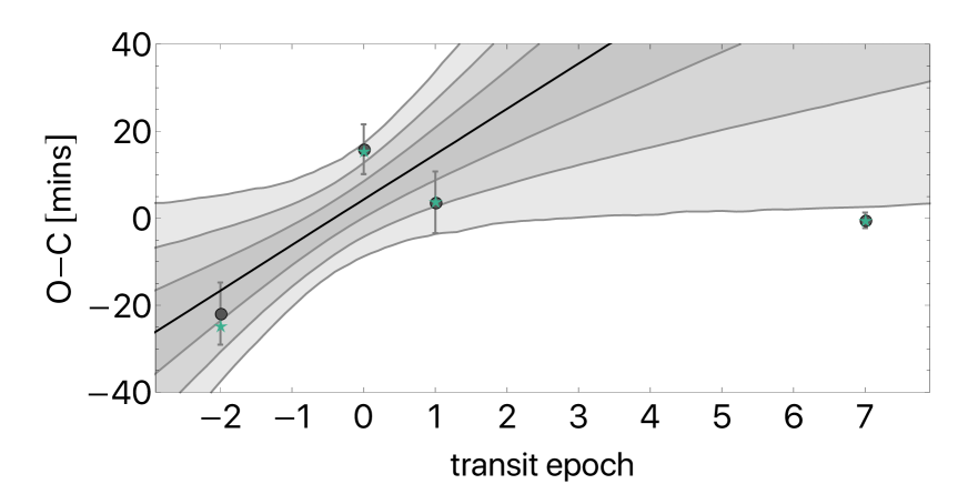
Figure S16: Transit timing variations. TTVs for Kepler-1625b, defined as observed times minus calculated times, where calculated times come from a linear ephemeris fit (model P) to all of the data marginalized over the various visit-long trend models attempted. The sloped line and three shaded regions represent the median, one-, two- and three-sigma credible intervals for the a posteriori linear ephemeris when conditioned upon the Kepler data alone, which reveals how deviant the HST epoch is. The green stars indicate the O-C values produced by the moon model, M.

Based on the Kepler data alone, we found that the P and T models had a Bayes factor of approximately unity (see Section 1.1 and Table LABEL:tab:kepler_evidences). Therefore, the first three transits observed appear compatible with a linear ephemeris. It is only the new HST transit which appears offset. However, including the HST epoch causes the maximum likelihood linear ephemeris to change substantially. This is visualized in Figure S16, where one can see the first three Kepler epoch times with the corresponding maximum a posteriori linear ephemeris plotted in black. The overall O-C diagram uses the updated maximum a posteriori ephemeris from model P using the HST data (marginalized over all of the visit-long trend models). Similarly, each transit time plotted (and also presented in Table LABEL:tab:ttvs) is that from a Bayesian model averaged posterior across the various visit-long trend models using model T (for details on the model averaging see Section 1.3.8). It is clear from main text Figure S16 that predicted Kepler-based prediction is inconsistent with the HST epoch with a one-sided $p$-value of $>3$ $\sigma$. For reference, each Kepler transit midtime has an uncertainty on the order of 10 minutes and the standard deviation on linear ephemeris predictions is 25.2 minutes derived from posterior samples. On this basis, we consider there to be a strong case for TTVs after introducing the HST epoch.

Against the maximum a posteriori linear ephemeris, the TTVs have a semi-amplitude of $\simeq 25$ minutes. With four transit times alone, is it perhaps not surprising that it is easy to find good solutions to the TTVs using an external perturber, although the solutions are extremely degenerate. We used TTVfaster  (?) with an MCMC exploration of the parameter space and found a wide range of plausible solutions assuming an external perturber.

1.3.4 Other timing effects

An important point is that no matter how well a perturbing planet can explain the observed TTVs, there are additional effects that an exomoon is expected to impart on a light curve that a perturbing planet, in general, will not. These are all the other photodynamical effects that may be seen in the transit of Kepler-1625b, such as transit duration variations  (?), transit impact parameter variations  (?) and transits of the moon itself  (?). Therefore, the way to establish whether a putative TTV is due to a moon or a perturbing planet is to look for these additional characteristic signatures expected from the presence of a moon.

Taking the dynamical signatures first, these are generally expected to be much smaller than the TTVs  (?), and accompanied by larger measurement errors (for example, transit durations have twice the uncertainty of transit times;  (?)). Given the fact that the TTVs are only significant at the 3 $\sigma$ level, we certainly do not expect, nor do we observe, noticeable duration variations. Nevertheless, these small effects are accounted for in a photodynamical model such as LUNA and thus we can see if they lead to any improvement in the fits. Model Z serves this purpose by fixing the moon radius to zero, but otherwise describing a full three-dimensional moon orbit with six more terms than model P.

It is instructive to compare the maximum likelihoods from models T and Z. Although our formalism for model T only uses two extra free parameters, as noted earlier in Section 1.3.2, this is somewhat artificial and in reality timing variations would require a planet described by six orbital parameters too. In this way, models T and Z can be directly compared as having essentially the same number of free parameters. Model Z consistently out-performs T in this regard. However, we consider these improvements as being necessary for any successful moon model rather than being convincing evidence in isolation. This is because model Z has greater flexibility than model T to explain light curve changes and thus in many ways is guaranteed to lead to an improvement. Nevertheless, the evidences show model Z consistently out-performs T by around $2\log K\simeq 4$, meaning there is some evidence favoring the moon hypothesis over a planet perturbation model. We caution that we have assumed planets do not induce short-period TDVs and/or impact parameter changes here but in some rare cases such changes have been detected (e.g.  (?, ?)).

1.3.5 The case for an exomoon

So far we have established that a) Kepler-1625b exhibits an early transit in the HST epoch indicating TTVs in the system, and b) a zero-radius moon model, which explains TDVs and other effects in addition to TTVs, leads to a modest improvement in the fits. A true exomoon would be expected to exhibit both points, and so while this is not convincing enough on its own, the exomoon hypothesis is certainly “on-track”. The next step is to consider the full planet+moon models.

We first note that model M, the full planet+moon model, is the favored hypothesis in each and every visit-long trend model attempted (see Table 1 of the main text), which already formally establishes the moon hypothesis as the leading candidate solution. With a strong case for TTVs already established (see Section 1.3.3), and some modest evidence for other moon-induced dynamical effects (Section 1.3.4), the mass signature of the putative moon is measurable and significant. To build a compelling case for an exomoon, we also need to detect the radius signature, since the dominant dynamical effect (TTVs) could be plausibly caused by a perturbing planet instead. Not only should we detect this radius signature, but that radius signature must be consistent with the moon solution in terms of both phase and physical parameters.

As a result of the strong TTV, model M has no other way to explain the timing offset except for using the moon, which leads to a positive $M_{S}/M_{P}$, which in turn demands a positive $R_{S}/R_{P}$ (due to our rejection of unphysical moon densities; see Section 1.3.2). Accordingly, inspection of the marginalized posterior distributions of $R_{S}/R_{P}$ is not a useful strategy for evaluating the case for a detection of the moon’s radius signature. The most direct method would be to directly compare the Bayes factor between the full moon model (i.e. model M) and an identical model for which the radius effect is turned off (i.e. model Z).

In all visit-long trend models attempted, we find that model M is favored over model Z. However, there is considerable range in the Bayes factors which result (see Table 2 of the main text). This can be linked to Figure 4 in the main text, where one can see that the high Bayes factor cases (e.g. linear) tend to correspond to cases where the moon transit is noticeably larger. In all cases, the moon transit occurs towards the end of the observations.

We would argue that a moon-like transit is immediately obvious even in the non-detrended data (see Figure 2 in the main text) and corresponds to the location where all of the moon models place the signal. This location is important because Kepler-1625b transits early in the HST epoch, for which we would therefore expect a corresponding moon to be transiting late. In other words, just combining the fact that we see an early transit along with the extra dip observed in the non-detrended data already presents a strong case for a self-consistent moon solution (and indeed our detailed modeling verifies this statement). Although the phasing is indeed aligned as expected then, this does not address whether the amplitude of the TTV (implying a certain moon mass) is compatible with the amplitude of the moon-like transit (implying a certain moon radius). We can therefore summarize the situation as being that the best explanation to the data is an exomoon, driven by a timing offset and moon-like dip with self-consistent phases, although the properties of the moon (in particular the size) appear to be dependent upon the trend model adopted and one (or all) of these may not be physically permissible. This latter point forms the subject of investigation in Section 1.3.6.

Before discussing whether the moon properties are physically sound or not, we briefly highlight that the $\chi^{2}$ improvement in going from model M to Z is quite high, ranging from 19.2 to 33.7 (note that we have $n=1048$ data points). On this basis, we find the SNR of the moon-like transits to be at least 19.

1.3.6 Evaluating the physicality of putative system parameters

We now have a TTV signal, modest evidence for other moon-induced dynamical effects and a sizable $\chi^{2}$ improvement when including the transit of a moon at the correct phase to explain the TTV. It is not yet clear, however, whether the candidate moon actually has physically sound parameters, beyond falling within the very generous density constraints imposed by our model (and described in Section 1.3.2).

Each trend model clearly leads to distinct moon parameters, as evident by the different moon depths in Figure 4 of the main text. Not only is the depth different, but the moon sometimes displays an egress feature and other times the egress occurs after the observations have ceased, which would require a greater planet-to-moon semi-major axis. Since the semi-major axis multiplied by the moon-to-planet ratio dictates the TTV amplitude, these longer semi-major axis solution necessarily require a smaller $M_{S}/M_{P}$. Furthermore, these longer semi-major axis solutions tend to be correlated to the greater moon transit depths as a result of the interplay with the trend model. This leads to a situation where $R_{S}/R_{P}$ and $M_{S}/M_{P}$ are somewhat anti-correlated between the various trend models, although admittedly there are just three models under inspection here.

The differing planet+moon transit parameters between each trend model imply different physical parameters then, with no guarantee of such parameters being necessarily physically plausible. To investigate this, we have to go from ratios to absolute dimensions. For the radius, this is easy. All solutions lead to good constraints on $R_{S}/R_{P}$ and $R_{P}/R_{\star}$ and since the stellar radius is known we can derive absolute sizes with reasonable precision.

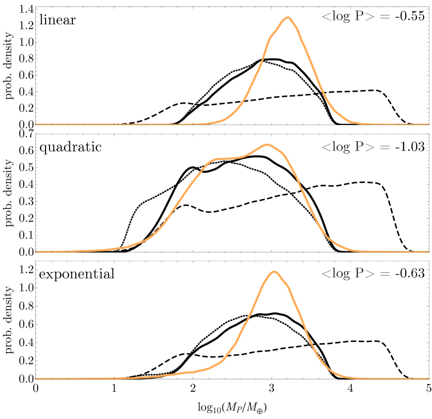
Figure S19: Mass constraints. Mass solutions for the planet from the various HST detrendings. The dotted lines represent the photodynamical posterior probability distribution while the dashed lines are posteriors generated by forecaster  (?). The solid black is the product of these probabilities. The orange lines represent the mass solution for the planet derived from that of the moon, which is well constrained based on the inferred radius. The mean likelihood, tracking the compatibility of the two solid curves, is shown in the upper-right corner.

Deriving absolute mass solutions is far trickier, since although $M_{S}/M_{P}$ is well-constrained from the TTVs, $M_{P}/M_{\star}$ is found to be only weakly constrained photodynamically in all models. This can be seen in Figure S19, by inspection of the dotted lines. In an attempt to shore-up this planetary mass measurement, we fed the absolute radius samples into the probabilistic empirical mass-radius relation forecaster  (?), which are the dashed lines in that plot. Taking the product of the two PDFs (using a Gaussian kernel density estimator) leads to the solid black posteriors in main text Figure S19, which represents one method of estimating the planetary mass from our data.

A second way to measure the planetary mass is to come from the exomoon side. Using the moon radius, we feed the samples into forecaster to get a moon mass and then convert that into a planetary mass using the $M_{S}/M_{P}$ distribution inferred by our fits. This second planetary mass solution is plotted in solid orange in Figure S19. A physically self-consistent solution would correspond to no tension between the two distributions. Visual inspection of Figure S19 reveals that the two estimates are consistent with one another for all three trend models, with the only difference being support for lower masses in the quadratic case.

To quantify the compatibility, we draw a random sample from one of the distributions (the moon-forecast based solution) and evaluated its likelihood using the product PDF from the other solution. We repeated this for all available samples ($\sim 40000$) and then evaluated the mean likelihood, which is reported in the top-right corners of Figure  S19. In agreement with simple inspection, the linear model appears to provide the greatest degree of physical self-consistency. All three provide broadly consistent mean likelihoods, none of which appear unphysical.

1.3.7 Combining the two mass estimates

Although the absolute dimensions of the system are constrained from photodynamics and our stellar properties, we are able to obtain more precise constraints by folding in the forecaster results from the previous paragraphs. For each trend model, we take the two planetary mass distributions (represented by the black solid and orange solid lines in Figure S19) and combine them to form a single planetary mass solution. This is achieved by taking the product of two PDFs and then defining the result as a likelihood function. We then sample from the function with a simple Markov Chain until 40,000 samples have been computed. The resulting planetary mass posterior is converted into a satellite mass using the $M_{S}/M_{P}$ parameter from the model M fits, which can be found in Table 2 of the main text.

1.3.8 Bayesian Model Averaging

The moon models display subtle but important variations in the associated parameters for each trend model. In contrast, we find the depths and transit times from model T are highly stable. In order to compile a single posterior for the transit times (presented in Table LABEL:tab:ttvs), we decided to marginalize over the three models using Bayesian Model Averaging.

The basic idea is that each model (in our case the three visit-long trend models) are assigned a weight based on their Bayesian evidence, $\mathcal{Z}$ (which is also known as the marginal likelihood). The odds-ratio between model $i$ and $j$ may be computed as

$O_{ij}=\exp(\log\mathcal{Z}_{i}^{\prime}-\log\mathcal{Z}_{j}^{\prime})$

And the final weights are now defined as

$w_{i}=\frac{O_{i1}}{\sum O_{i1}},$

such that $\sum w_{i}=1$. With the weights assigned, we draw a random integer from a multinomial distribution using the weights vector to choose a model. We then choose a random posterior sample from that model and append it to a new array. After many iterations, we construct a Bayesian Model Averaged posterior for model T.

We repeated this process on the nine spectral channels computed earlier using model T with the three trend models. The resulting marginalized ratio-of-radii is treated as our final spectral retrieval for Kepler-1625b and is presented in Table LABEL:tab:spectrum.

1.3.9 Stability Analysis

Moons are generally considered stable if they reside beyond the Roche limit and within $\sim$ 0.4895 $R_{Hill}$ for prograde moons and 0.9309 $R_{Hill}$ for retrograde moons  (?). Our solutions place the moon at $a_{s}=0.265_{-0.081}^{+0.123}$, $0.275_{-0.095}^{+0.126}$, and $0.258_{-0.081}^{+0.111}\;R_{Hill}$ for the linear, quadratic, and exponential models, respectively.

However, satellites on inclined orbits may be less stable over the long term. Our three moon solutions all suggest significant inclinations with respect to the planet’s orbital plane, so we carry out a stability analysis using the analytical formula provided by  (?). Drawing from our joint model posteriors we find the moon solution has a stable configuration for $73.1\%$ of the draws with the linear model, $73.6\%$ of the time for the quadratic model, and $78.3\%$ of the time for the exponential model.

1.3.10 Analysis of Residuals

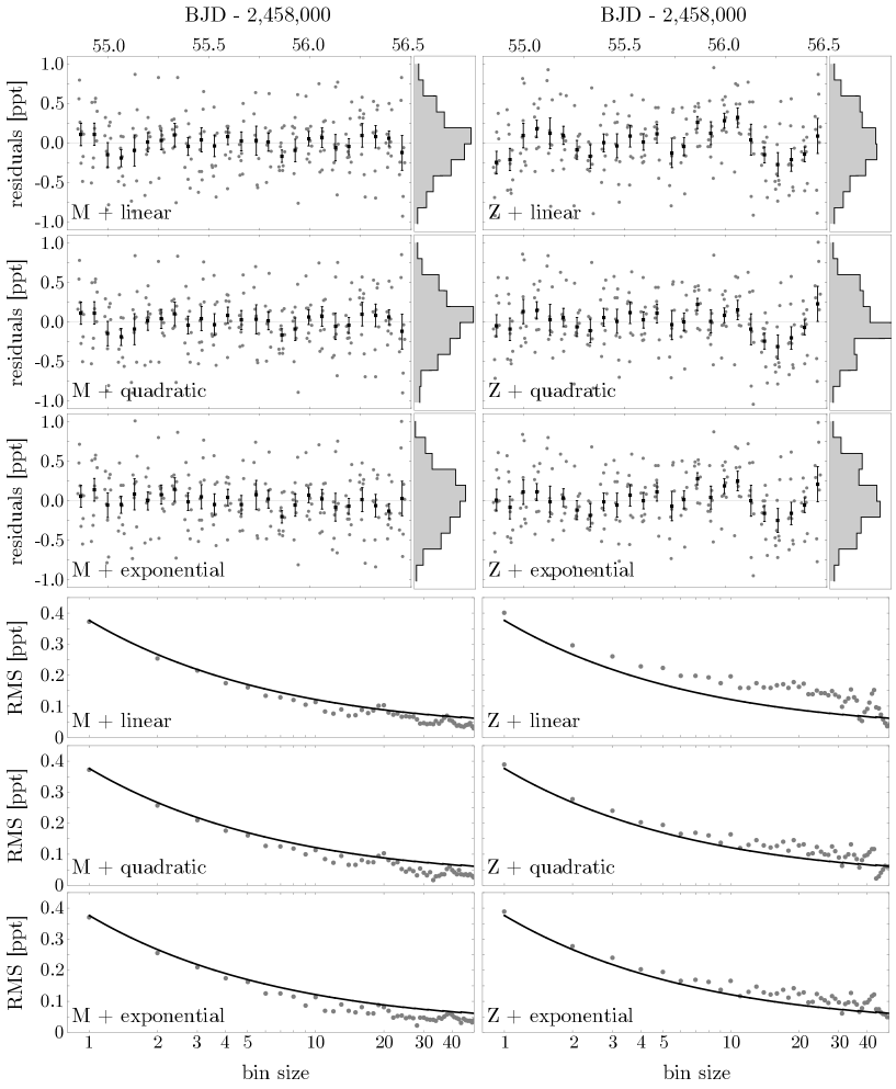
Figure S17: Residual analysis. Analysis of the white light curve from WFC3 residuals for six different models. Upper six panels show the photometric residuals, with orbit binned points, alongside a histogram of the unbinned scatter. Lower panels show the root mean square (RMS) as a function of bin size, where the solid line is that expected for pure Gaussian noise equal to the assumed photometric noise in our fits. In both sets, excess noise in the Z-models is visible, caused by the moon-like dip being ignored in those fits.

As an extra check, we here describe an analysis of the light curve residuals. Strong time-correlated noise structure could potentially explain the moon-like dip without invoking a satellite. In total, we considered six sets of relevant residuals, the three trend models applied to the moon model, M, and the same three applied to the zero-radius moon model, Z. These are shown in Figure S17.

The M model residuals appear consistent with Gaussian noise, displaying no obvious trends or time-correlated structure. In contrast, the Z models consistently fail to explain the moon-like dip leading to a noticeable excursion in the residuals at this time.

We binned the residuals into progressively larger bins and monitored the effect this has on the root mean square (RMS). Gaussian residuals would be expected to bin as $\sigma_{n}=\sigma_{1}n^{-1/2}\sqrt{m/(m-1)}$, where $n$ is the number of points binned, $m$ is the number of bins and $\sigma_{1}$ is the RMS of the unbinned data.

Setting $\sigma_{1}$ to our standard photometric error, derived from our hook correction procedure, reveals that this curve yields a close match to the M model residuals (see lower panels of Figure S17). If anything, the noise appears to behave even better than Gaussian suggesting that we have slightly overestimated our standard uncertainty value.

In contrast, all three Z models show excess power at large bin sizes, indicative of time-correlated structure in the residuals. This structure must be caused by the moon-like dip since models M and Z are otherwise identical.

In summary, our analysis of the residuals adds weight to the case that the moon-like dip is a real feature in the data.

1.3.11 Chromatic test

In Section 1.2.10, we discussed how inspection of the comparison star’s photometry and the centroids revealed no evidence to suspect the moon-like dip is an instrumental artifact. A third test, mentioned in that section, was to consider if the dip was chromatic in nature. An exomoon transit might be expected to be slightly chromatic due to the atmosphere, but large transit depth variations would be indicative of a blend or some previously unexplained instrumental effect. Accordingly, we here describe a brief investigation into this possibility.

Already we have discussed how spectral elements can be extracted by dividing the white light curve aperture up into slices (see Section 1.2.11). As a result of dividing up the aperture in this way, the noise naturally increases in each channel. For the sake of testing if the moon-like dip is chromatic or not, we only require two different colors, allowing us to use broader slices with higher precision. Accordingly, we decided to split up the optimal aperture into two colors for a chromatic test.

When divided into ten slices, we found that the reddest and bluest channels displayed less stable photometry, likely as a result of the sharp drop off in WFC3’s sensitivity towards the wavelength extremes. For this test then, we elected to omit those most extreme channels and ultimately took the central two-thirds of the aperture, split into two, as our two colors. This led to a “blue” channel defined from columns 476 to 518 (inclusive) and a “red” channel from 519 to 561, which corresponds to 1.2-1.4$\mu$m and 1.4-1.6$\mu$m respectively.

We first independently correct for the hooks using the same method as described in Section 1.2.6. The white light curve led to a final inter-orbit RMS of 375.5 ppm, the blue and red channels here yielded 598.8 ppm and 612.8 ppm respectively. This is slightly better than the naive $\sqrt{3}$ scaling one would expect if the product of the source and WFC3 had a perfectly flat wavelength response, reflecting how the response actually peaks in the center and drops off towards the edges.

With the chromatic photometry in hand, our objective is now to test whether each channel is more consistent with either the model including or excluding an exomoon transit; formally models M and Z. To accomplish this, we took the maximum a posteriori solution from model M and plotted the light curve morphology with the trend parameters turned off, thus creating a “template” of the moon solution. We then multiplied this template by a trend model with unset trend parameters. These unknown trend parameters were then fit by regressing (least squares) the template multiplied by the trend model to the blue/red channel photometry. By doing this, we allow for the fact that the visit-long trend model is itself chromatic. Since there are three possible trend models considered in this work, we tried all three and selected the best one, since it was clear sometimes a particular trend model was a poor representation of the data. It is interesting to note that the quadratic trend won out every time.

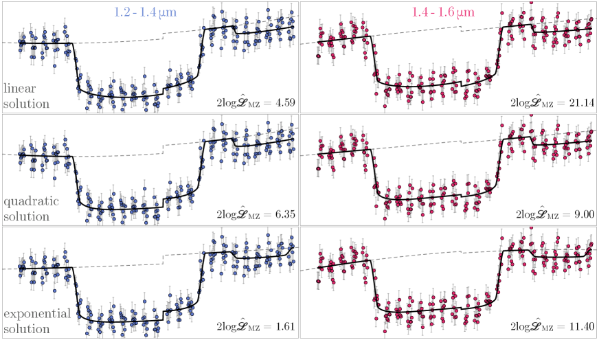
Figure S18: Chromatic test. Tests to see if the moon-like dip is present in two independent spectral regions of the WFC3 bandpass (each column). Each row shows our maximum a posteriori moon model (model M) plotted in black, multiplied by a simple trend model regressed to each channel. Since we have three different moon models depending on which trend model is used on the white light curve, we show all three (one per row). In every case, these templates give a closer match to the data than those resulting from model Z (no moon transit).

One complication with the above is that there is not a single moon model template, but rather three - since we originally attempted three trend models and have been unable to definitively select a single model. We therefore repeated the above the templates resulting from M + linear, M + quadratic and M + exponential trends. This was done for both the blue and red channel data, and in each case we recorded the (six) resulting $\chi^{2}$ values of the (three) trend-regressed templates. We then repeated the entire excercise using the Z model templates, which do not allow for an exomoon transit. The results, including a comparison of the $\chi^{2}$ values, is shown in Figure S18.

In all six cases, the moon template provides a closer match to the red/blue channel data than the Z model. Although the moon model appears favored in every case, the red channel does appear to yield a more significant preference.

In general, one should expect the red channel to be less affected by stellar activity, such as rotating star spots, plages, granulation and micro-flares. If the blue channel, which is more sensitive to such effects, were to exhibit a stronger preference for a moon-like dip, this could have been a cause for concern. As it stands, however, the results appear to be consistent with an overall preference for model M over Z.

We also fitted the two channels with independent Z and M models using the same procedure as for the white light curve. In all six cases (three trends, two channels), the moon model is favored over model Z with evidences of $1.51\pm 0.31$, $1.84\pm 0.31$ and $3.78\pm 0.31$ for the blue channel and $6.68\pm 0.32$, $2.59\pm 0.32$ and $4.58\pm 0.31$ for the red, where the three numbers correspond to $2\log(\mathcal{Z}_{M}/\mathcal{Z}_{Z})$ for the linear, quadratic and exponential trends, respectively. We do note that the solutions are less well-converged than before, as a result of the reduced precision, with credible intervals inflating by up to a few times.

In conclusion, the moon-like dip occurring post-egress is statistically favored in both the red and blue channels and appears consistent with the solution derived from the white light curve alone.

1.3.12 Predictions

As noted in the main text, we consider that future observations will be critical in assessing the true nature of Kepler-1625b and the reality of the exomoon signature. To this end, we took 100 random samples from our model M posteriors and used them to predict the morphology of the next transit event in May 2019 (epoch 9). This prediction is shown in Figure S22. The model suggests a high likelihood of observing a pre-transit feature due to the exomoon and thus we strongly encourage observations around this time.

Supplementary Figures and Tables

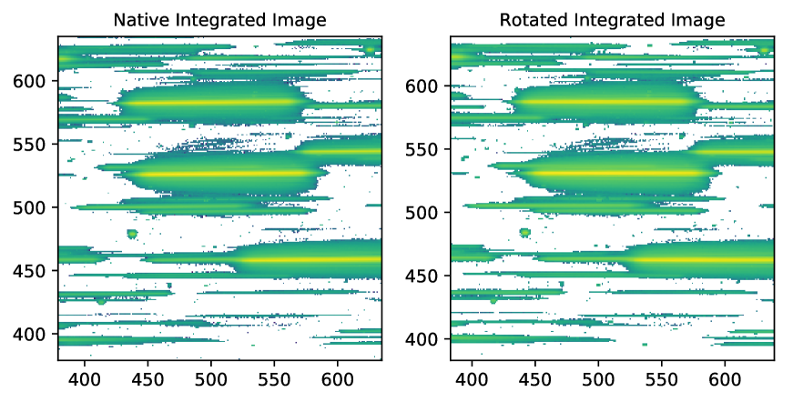
Figure S8: HST image rotation. Left:Integrated HST image with the spectra natively inclined 0.5 degrees with respect to the $x$-axis. Right: the rotated image for simplifying the spectral extraction. Pixel values are logarithmic to show the full extent of the spectra; white space indicates backgrounds integrating to values $<0$, for which the logarithm is undefined.

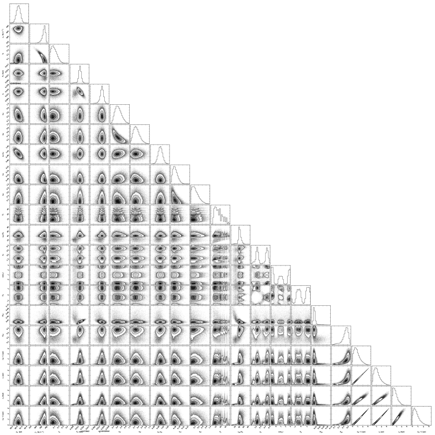
Figure S20: Model posteriors. Model posteriors of the parameters explored in the moon model. Shown here the results from the exponential trend model.

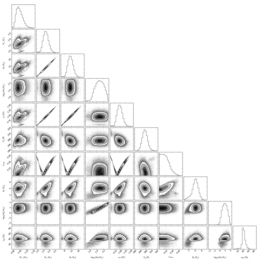
Figure S21: Physical posteriors. Physical system parameter posteriors derived from the exponential model results.

Figure S22: The May 2019 transit. Predictions for the May 2019 transit of Kepler-1625 assuming the planet-moon model is correct. 100 random draws from each of the three instrumental trend model posteriors are overlaid showing broad consistency between the three model predictions.

Table S1: Kepler-only fits. P for planet model. T for planetary TTV model. Z for a zero-radius moon model. M for moon model.

model	$\log\mathcal{Z}$	$\log\hat{\mathcal{L}}$
$\mathrm{P}$	$4924.84\pm 0.07$	$4950.26$
$\mathrm{T}$	$4924.38\pm 0.08$	$4954.38$
$\mathrm{Z}$	$4927.53\pm 0.08$	$4956.42$
$\mathrm{M}$	$4925.34\pm 0.08$	$4959.59$
$\mathrm{M}-\mathrm{P}$	$0.50\pm 0.11$	$9.33$
$\mathrm{M}-\mathrm{T}$	$0.96\pm 0.11$	$5.22$
$\mathrm{M}-\mathrm{Z}$	$-2.19\pm 0.11$	$3.17$

Table S2: Transmission spectrum. Marginalized ratio-of-radii derived from a Bayesian model averaged joint-posteriors of the linear, quadratic and exponential HST detrending models, using the averaged (“AVG”) Kepler data detrending model.

$\lambda$	$\Delta\lambda$	$R_{P}/R_{\star}$	$\sigma_{R_{P}/R_{\star}}$
0.65	0.200	0.06102	0.0008
1.135	0.027	0.06438	0.0015
1.192	0.025	0.06198	0.0015
1.252	0.027	0.05770	0.0017
1.310	0.024	0.06157	0.0015
1.368	0.028	0.05960	0.0014
1.426	0.026	0.05990	0.0017
1.485	0.027	0.05924	0.0019
1.543	0.023	0.06019	0.0020
1.600	0.027	0.05910	0.0026

Table S3: Transit timings. Marginalized transit times derived from a Bayesian model averaged joint-posteriors of the linear, quadratic and exponential HST detrending models, using the averaged (“AVG”) Kepler data detrending model.

Epoch	$\tau$	O-C [mins]
-2	$55469.2037_{-0.0049}^{+0.0048}$	$-21.9_{-7.1}^{+7.1}$
0	$56043.9715_{-0.0040}^{+0.0040}$	$+15.9_{-5.8}^{+5.6}$
1	$56331.3337_{-0.0051}^{+0.0049}$	$+3.7_{-7.2}^{+7.0}$
7	$58055.5563_{-0.0014}^{+0.0013}$	$-0.4_{-1.8}^{+1.7}$

References and Notes

- 1. Han, C., Han, W. 2002. On the Feasibility of Detecting Satellites of Extrasolar Planets via Microlensing. The Astrophysical Journal 580, 490.
- 2. Han, C. 2008. Microlensing detections of moons of exoplanets. The Astrophysical Journal 684, 684.
- 3. Liebig, C. 2010. Detectability of Extrasolar Moons as Gravitational Microlenses. Astronomy & Astrophysics 520, 68.
- 4. Cabrera, J., Schneider, J. 2007. Detecting companions to extrasolar planets using mutual events. Astronomy and Astrophysics 464, 1133.
- 5. Agol, E., Jansen, T., Lacy, B., Robinson, T. D., Meadows, V. 2015. The Center of light: Spectroastrometric detection of exomoons. The Astrophysical Journal 812, 5.
- 6. Noyola, J. P., Satyal, S., Musielak, Z. E. 2014. Detection of Exomoons through Observation of Radio Emissions. The Astrophysical Journal 791, 25.
- 7. Lewis, K. M., Sackett, P. D., Mardling, R. A. 2008. Possibility of Detecting Moons of Pulsar Planets through Time-of-Arrival Analysis. The Astrophysical Journal 685, L153.
- 8. Sartoretti, P., Schneider, J. 1999. On the detection of satellites of extrasolar planets with the method of transits. Astronomy and Astrophysics Supplement Series 134, 553.
- 9. Kipping, D. M. 2009. Transit timing effects due to an exomoon. Monthly Notices of the Royal Astronomical Society 392, 181.
- 10. Kipping, D. M. 2009. Transit timing effects due to an exomoon - II. Monthly Notices of the Royal Astronomical Society 396, 1797.
- 11. Barclay, T., and 57 colleagues 2013. A sub-Mercury-sized exoplanet. Nature 494, 452.
- 12. Teachey, A., Kipping, D. M., Schmitt, A. R. 2018. HEK. VI. On the dearth of Galilean analogs in Kepler, and the exomoon candidate Kepler-1625b I. The Astronomical Journal 155, 36.
- 13. Namouni, F. 2010. The Fate of Moons of Close-in Giant Exoplanets. The Astrophysical Journal 719, L145.
- 14. Spalding, C., Batygin, K., Adams, F. C. 2016. Resonant Removal of Exomoons during Planetary Migration. The Astrophysical Journal 817, 18.
- 15. Morton, T. D., and 7 colleagues 2016. False Positive Probabilities for all Kepler Objects of Interest: 1284 Newly Validated Planets and 428 Likely False Positives. The Astrophysical Journal 822, 86.
- 16. Mathur, S., and 16 colleagues 2017. Revised Stellar Properties of Kepler Targets for the Q1-17 (DR25) Transit Detection Run. The Astrophysical Journal Supplement Series 229, 30.
- 17. Jenkins, J. M., and 29 colleagues 2010. Overview of the Kepler Science Processing Pipeline. The Astrophysical Journal 713, L87.
- 18. Kipping, D. M., Hartman, J., Buchhave, L. A., Schmitt, A. R., Bakos, G. Á., Nesvorný, D. 2013. The Hunt for Exomoons with Kepler (HEK). II. Analysis of Seven Viable Satellite-hosting Planet Candidates. The Astrophysical Journal 770, 101.
- 19. Stumpe, M. C., and 10 colleagues 2012. Kepler Presearch Data Conditioning I—Architecture and Algorithms for Error Correction in Kepler Light Curves. Publications of the Astronomical Society of the Pacific 124, 985.
- 20. Smith, J. C., and 10 colleagues 2012. Kepler Presearch Data Conditioning II - A Bayesian Approach to Systematic Error Correction. Publications of the Astronomical Society of the Pacific 124, 1000.
- 21. Kipping, D. M. 2011. LUNA: an algorithm for generating dynamic planet-moon transits. Monthly Notices of the Royal Astronomical Society 416, 689.
- 22. Agol, E., and 6 colleagues 2010. The Climate of HD 189733b from Fourteen Transits and Eclipses Measured by Spitzer. The Astrophysical Journal 721, 1861.
- 23. Berta, Z. K., and 9 colleagues 2012. The Flat Transmission Spectrum of the Super-Earth GJ1214b from Wide Field Camera 3 on the Hubble Space Telescope. The Astrophysical Journal 747, 35.
- 24. Wakeford, H. R., Sing, D. K., Evans, T., Deming, D., Mandell, A. 2016. Marginalizing Instrument Systematics in HST WFC3 Transit Light Curves. The Astrophysical Journal 819, 10.
- 25. Huitson, C. M., and 16 colleagues 2013. An HST optical-to-near-IR transmission spectrum of the hot Jupiter WASP-19b: detection of atmospheric water and likely absence of TiO. Monthly Notices of the Royal Astronomical Society 434, 3252.
- 26. Ranjan, S., and 6 colleagues 2014. Atmospheric Characterization of Five Hot Jupiters with the Wide Field Camera 3 on the Hubble Space Telescope. The Astrophysical Journal 785, 148.
- 27. Knutson, H. A., and 9 colleagues 2014. Hubble Space Telescope Near-IR Transmission Spectroscopy of the Super-Earth HD 97658b. The Astrophysical Journal 794, 155.
- 28. Stevenson, K. B., and 7 colleagues 2014. Transmission Spectroscopy of the Hot Jupiter WASP-12b from 0.7 to 5 m. The Astronomical Journal 147, 161.
- 29. Stevenson, K. B., Bean, J. L., Fabrycky, D., Kreidberg, L. 2014. A Hubble Space Telescope Search for a Sub-Earth-sized Exoplanet in the GJ 436 System. The Astrophysical Journal 796, 32.
- 30. Seager, S., Sasselov, D. D. 2000. Theoretical Transmission Spectra during Extrasolar Giant Planet Transits. The Astrophysical Journal 537, 916.
- 31. de Wit, J., Seager, S. 2013. Constraining Exoplanet Mass from Transmission Spectroscopy. Science 342, 1473.
- 32. Feroz, F., Hobson, M. P. 2008. Multimodal nested sampling: an efficient and robust alternative to Markov Chain Monte Carlo methods for astronomical data analyses. Monthly Notices of the Royal Astronomical Society 384, 449.
- 33. Feroz, F., Hobson, M. P., Bridges, M. 2009. MULTINEST: an efficient and robust Bayesian inference tool for cosmology and particle physics. Monthly Notices of the Royal Astronomical Society 398, 1601.
- 34. Kass, R. E. & Raftery, A. E. 1995. Bayes Factors. Journal of the American Statistical Association, 90, 773.
- 35. Chen, J., Kipping, D. 2017. Probabilistic Forecasting of the Masses and Radii of Other Worlds. The Astrophysical Journal 834, 17.
- 36. Kipping, D. M. 2010. How to weigh a star using a moon. Monthly Notices of the Royal Astronomical Society 409, L119.
- 37. Kempton, E. M.-R., Lupu, R., Owusu-Asare, A., Slough, P., Cale, B. 2017. Exo-Transmit: An Open-Source Code for Calculating Transmission Spectra for Exoplanet Atmospheres of Varied Composition. Publications of the Astronomical Society of the Pacific 129, 44402.
- 38. Agnor, C. B., Hamilton, D. P. 2006. Neptune’s capture of its moon Triton in a binary-planet gravitational encounter. Nature 441, 192.
- 39. Berger, T. A., Huber, D., Gaidos, E., van Saders, J. L. 2018. Revised Radii of Kepler Stars and Planets using Gaia Data Release 2. ArXiv e-prints arXiv:1805.00231.
- 40. Cilibrasi, M., Szulágyi, J., Mayer, L., Drażkowska, J., Miguel, Y., Inderbitzi, P. 2018. Satellites Form Fast & Late: a Population Synthesis for the Galilean Moons. ArXiv e-prints arXiv:1801.06094.
- 41. Ochiai, H., Nagasawa, M., Ida, S. 2014. Extrasolar Binary Planets. I. Formation by Tidal Capture during Planet-Planet Scattering. The Astrophysical Journal 790, 92.
- 42. Kipping, D. M., Huang, X., Nesvorný, D., Torres, G., Buchhave, L. A., Bakos, G. Á., Schmitt, A. R. 2015. The Possible Moon of Kepler-90g is a False Positive. The Astrophysical Journal 799, 14.
- 43. Dalba, P. A., Muirhead, P. S., Croll, B., Kempton, E. M.-R. 2017. Kepler Transit Depths Contaminated By a Phantom Star. The Astronomical Journal 153, 59.
- 44. Bryson, S. T., and 10 colleagues 2010. The Kepler Pixel Response Function. The Astrophysical Journal 713, L97.
- 45. Schlafly, E. F., Finkbeiner, D. P. 2011. Measuring Reddening with Sloan Digital Sky Survey Stellar Spectra and Recalibrating SFD. The Astrophysical Journal 737, 103.
- 46. Kümmel, M., Walsh, J. R., Pirzkal, N., Kuntschner, H., Pasquali, A. 2009. The Slitless Spectroscopy Data Extraction Software aXe. Publications of the Astronomical Society of the Pacific 121, 59.
- 47. Bertin, E., Arnouts, S. 2010. SExtractor: Source Extractor. Astrophysics Source Code Library ascl:1010.064.
- 48. Kümmel, M., Kuntschner, H., Walsh, J. R., Bushouse, H. 2011. Master sky images for the WFC3 G102 and G141 grisms.Space Telescope WFC Instrument Science Report.
- 49. Jones, E., Oliphant, T., Peterson, P., et al. 2001, http://www.scipy.org
- 50. Deming, D., and 20 colleagues 2013. Infrared Transmission Spectroscopy of the Exoplanets HD 209458b and XO-1b Using the Wide Field Camera-3 on the Hubble Space Telescope. The Astrophysical Journal 774, 95.
- 51. Deming, D., Harrington, J., Seager, S., Richardson, L. J. 2006. Strong Infrared Emission from the Extrasolar Planet HD 189733b. The Astrophysical Journal 644, 560.
- 52. Knutson, H. A., and 8 colleagues 2007. A map of the day-night contrast of the extrasolar planet HD 189733b. Nature 447, 183.
- 53. Charbonneau, D., and 7 colleagues 2008. The Broadband Infrared Emission Spectrum of the Exoplanet HD 189733b. The Astrophysical Journal 686, 1341.
- 54. Freedman, R. S., Marley, M. S., Lodders, K. 2008. Line and Mean Opacities for Ultracool Dwarfs and Extrasolar Planets. The Astrophysical Journal Supplement Series 174, 504.
- 55. Freedman, R. S., Lustig-Yaeger, J., Fortney, J. J., Lupu, R. E., Marley, M. S., Lodders, K. 2014. Gaseous Mean Opacities for Giant Planet and Ultracool Dwarf Atmospheres over a Range of Metallicities and Temperatures. The Astrophysical Journal Supplement Series 214, 25.
- 56. Lupu, R. E., and 8 colleagues 2014. The Atmospheres of Earthlike Planets after Giant Impact Events. The Astrophysical Journal 784, 27.
- 57. Luri, X., Brown, A. G. A., Sarro, L. M., et al. 2018, “Gaia Data Release 2: using Gaia parallaxes”, arXiv e-print:1804.09376
- 58. Morton, T. 2015, isochrones: Stellar model grid package, Astrophysics Source Code Library.
- 59. Foreman-Mackey, D., Hogg, D. W., Lang, D., Goodman, J. 2013, “emcee: The MCMC Hammer”, PASP, 125, 306.
- 60. Huber, D., Bryson, S. T., Haas, M. R., et al. 2016, “The K2 Ecliptic Plane Input Catalog (EPIC) and Stellar Classifications of 138,600 Targets in Campaigns 1-8”, ApJS, 224, 2.
- 61. Kipping, D. M., Bakos, G. Á., Buchhave, L., Nesvorný, D., Schmitt, A. 2012. The Hunt for Exomoons with Kepler (HEK). I. Description of a New Observational project. The Astrophysical Journal 750, 115.
- 62. Skilling, J. 2004. Nested Sampling. American Institute of Physics Conference Series 395.
- 63. Kipping, D. M. 2013. Efficient, uninformative sampling of limb darkening coefficients for two-parameter laws. Monthly Notices of the Royal Astronomical Society 435, 2152.
- 64. Kipping D. M., Forgan, D., Hartman, J., Nesvorný, D., Bakos, G. Á., Schmitt, A. R., Buchhave, L. A. 2013, Astrophys. J., 777, 134
- 65. Kipping, D. M., and 7 colleagues 2015. The Hunt for Exomoons with Kepler (HEK): V. A Survey of 41 Planetary Candidates for Exomoons. The Astrophysical Journal 813, 14.
- 66. Agol, E., Deck, K. 2016. TTVFaster: First order eccentricity transit timing variations (TTVs). Astrophysics Source Code Library ascl:1604.012.
- 67. Carter, J. A., Yee, J. C., Eastman, J., Gaudi, B. S., Winn, J. N. 2008. Analytic Approximations for Transit Light-Curve Observables, Uncertainties, and Covariances. The Astrophysical Journal 689, 499.
- 68. Nesvorný, D., Kipping, D., Terrell, D., Hartman, J., Bakos, G. Á., Buchhave, L. A. 2013. KOI-142, The King of Transit Variations, is a Pair of Planets near the 2:1 Resonance. The Astrophysical Journal 777, 3.
- 69. Szabó, G. M., Pál, A., Derekas, A., Simon, A. E., Szalai, T., Kiss, L. L. 2012. Spin-orbit resonance, transit duration variation and possible secular perturbations in KOI-13. Monthly Notices of the Royal Astronomical Society 421, L122.
- 70. Kipping, D. M. 2014. Characterizing distant worlds with asterodensity profiling. Monthly Notices of the Royal Astronomical Society 440, 2164.
- 71. Domingos, R. C., Winter, O. C., & Yokoyama, T. 2006, Mon. Not. R. Astron. Soc., 373, 1227.
- 72. Donnison, J. R. 2014, Earth Moon and Planets, 113, 73.