Machine learning electron correlation in a disordered medium

Abstract

Learning from data has led to a paradigm shift in computational materials science. In particular, it has been shown that neural networks can learn the potential energy surface and interatomic forces through examples, thus bypassing the computationally expensive density functional theory calculations. Combining many-body techniques with a deep learning approach, we demonstrate that a fully-connected neural network is able to learn the complex collective behavior of electrons in strongly correlated systems. Specifically, we consider the Anderson-Hubbard (AH) model, which is a canonical system for studying the interplay between electron correlation and strong localization. The ground states of the AH model on a square lattice are obtained using the real-space Gutzwiller method. The obtained solutions are used to train a multi-task multi-layer neural network, which subsequently can accurately predict quantities such as the local probability of double occupation and the quasiparticle weight, given the disorder potential in the neighborhood as the input.

Machine learning (ML) mitchell97 ; scholkopf02 ; nielsen15 is one of today’s most rapidly growing interdisciplinary fields. The deep-learning neural network (NN) provides a powerful universal method for finding patterns and regularities in high-dimensional data duda01 ; bishop06 . It has found successful applications in a wide variety of fields. In condensed-matter physics and materials science, notable applications include using ML to guide materials design sumpter96 ; kalinin15 ; balachandran18 and for identification and classification of crystalline structures reinhart17 ; dietz17 ; lubbers17 ; cubuk15 ; schoenholz16 . Recently, ML techniques have also been taken up by researchers in the area of strongly correlated systems. The majority of such activities focus on using ML to identify phases and phase transitions in many-body systems ranging from classical statistical models wang16 ; carrasquilla17 ; wetzel17 ; hu17 and quantum fermionic Hamiltonians chng17 ; broecker17 to topological phases zhang17 and many-body localization schindler17 . In these studies, a deep-learning NN, trained with data from classical or quantum Monte Carlo simulations, is shown to be able to correctly distinguish phases and predict phase diagrams. ML trained NNs can also represent thermodynamic phases in equilibrium (Boltzmann machines) torlai16 , or ground-state wavefunctions of quantum many-body systems carleo17 ; deng17 .

In this paper, we demonstrate another application of ML in correlated electron systems, namely using NN as an efficient emulator for many-body problem solvers. Specifically, our goal is to investigate whether deep-learning NN can be trained to predict electron correlation, such as the probability of double-occupation, in a disordered medium. Our approach here is similar in spirit to those adopted in quantum chemistry and materials science communities, where the ML trained NN is used to bypass the time-consuming density functional theory (DFT) calculations brockherde17 ; snyder12 ; snyder13 ; li16 ; yao16 ; li16b ; schutt17 . Such activities have led to the fast prediction of molecular atomization energies rupp12 ; hansen13 and efficient parametrization of interatomic force fields behler07 ; bartok10 ; li15 ; botu15 ; chmiela17 , to name a few. We note in passing that similar ideas of bypassing expensive numerical calculations with ML model have also been explored in correlated electron systems, such as using ML to replace the impurity solver for DMFT arsenault14 , or to speed up total energy calculation in Monte Carlo simulations liu17 ; xu17 ; huang17 .

Model and Method. We consider the disordered Hubbard model in two dimensions:

$$\mathcal{H}=-t\sum_{ij,\sigma}\hat{c}^{\dagger}_{i,\sigma}\hat{c}^{\;}_{j,\sigma}+\sum_{i,\sigma}\epsilon_{i}\hat{n}^{\;}_{i,\sigma}+U\sum_{i}\hat{n}_{i,\uparrow}\hat{n}_{i,\downarrow}$$ (1)

where $\hat{c}^{\dagger}_{i,\sigma}$ is the electron creation operator with spin $\sigma=\uparrow,\downarrow$ at site-$i$, and $\hat{n}_{i,\sigma}\equiv\hat{c}^{\dagger}_{i,\sigma}\hat{c}^{\;}_{i,\sigma}$ is the corresponding number operator . The first-term describes nearest-neighbor hopping of electrons. The second term denotes the random local potential. The last term is the on-site Hubbard repulsion. As in the standard Anderson model, here the site energy $\epsilon_{i}$ is a random number drawn uniformly from the interval $[-W/2,+W/2]$. We work at half-filling on an $L\times L$ square lattice with periodic boundary conditions. The Hamiltonian Eq. (1), also known as the Anderson-Hubbard (AH) model, is considered a paradigmatic model for studying the interplay between strong electron correlation and disorder.

The AH model has been intensively studied by several numerical methods, including Hatree-Fock calculations heidarian04 ; shinaoka09 , quantum Monte Carlo simulations ulmke95 ; ulmke97 ; pezzoli09 ; pezzoli10 , and extended dynamical mean field theory (DMFT) dobrosavljevic97 ; dobrosavljevic03 ; byczuk05 ; aguiar09 . In particular, intrinsic metal-insulator transition without magnetic order can be quantitatively calculated within the DMFT framework georges96 . For application to disordered systems, DMFT can be readily combined with the typical medium theory (TMT) in which a geometrically averaged local density of states is used to construct the electron bath dobrosavljevic03b . The non-magnetic phase diagram of AH model obtained from the TMT-DMFT method includes three distinct phases: a correlated metallic phase, a Mott insulating phase, and an Anderson insulating phase byczuk05 ; aguiar09 . Importantly, the two insulating phases of the AH model have very different characters. The Mott insulator results from the strong correlation effect which prohibits electrons from hopping to the neighboring sites. On the other hand, strong disorder weakens the constructive interference that allows an electron wave packet to propagate coherently in a periodic potential, leading to the Anderson insulator. TMT-DMFT calculation shows that these two insulating phases are continuously connected byczuk05 ; aguiar09 .

Real-space approaches such as variational Monte Carlo (VMC) simulations pezzoli09 ; pezzoli10 , statistical DMFT dobrosavljevic97 ; tanaskovic03 , and the Gutzwiller methods andrade09 ; andrade10 can better cope with the crucial spatial fluctuations in low dimensional systems. Applying VMC to the 2D AH model finds a continuous transition that separates the Mott insulator from the Anderson insulator in the non-magnetic phase diagram pezzoli09 ; pezzoli10 . It is worth noting that there is no sharp distinction between correlated metal and Anderson insulator in 2D. Interestingly, detailed large-scale simulations of the 2D AH model within the Brinkman-Rice formalism, where the efficient Gutzwiller method can be applied, showed that strong spatial inhomogeneity gives rise to an electronic Griffiths phase that precedes the metal-insulator transition andrade09 .

Here we employ the Gutzwiller method to solve the AH model on a square lattice. In its original formulation, a variational wavefunction $|\Psi_{G}\rangle=\mathcal{P}_{G}|\Psi_{0}\rangle$ is constructed by applying a real-space projector $\mathcal{P}_{G}=\prod_{i}\mathcal{P}_{i}$ on the Slater determinant $|\Psi_{0}\rangle$ obtained from the non-interacting electron Hamiltonian gutzwiller63 . Optimization of $|\Psi_{G}\rangle$ can be efficiently carried out with the so-called Gutzwiller approximation (GA) gutzwiller63 , which becomes exact in the infinite dimension limit. Moreover, GA corresponds to the zero-temperature saddle point solution of the slave-boson (SB) method kotliar86 . Indeed, by factoring out the occupation probability $P^{0}_{i}$ of the uncorrelated state, the local projector can be expressed as $\mathcal{P}_{i}\equiv\sum_{\alpha,\beta}\Phi_{i,\alpha\beta}/(P^{0}_{i,\beta})^{-1/2}|\alpha\rangle\langle\beta|$, where $\alpha$, $\beta$ are the local many-electron state, and the elements of the variational matrix $\Phi_{i}$ correspond to the SB coherent-state amplitude lanata12 ; lanata15 . For single-band Hubbard model, $\Phi_{i}$ is a diagonal matrix of dimension 4, i.e. $\Phi_{i}={\rm diag}(e_{i},p_{i,\uparrow},p_{i,\downarrow},d_{i})$, and the square of these diagonal elements corresponds to the probability of empty, single (with spin $\sigma=\uparrow,\downarrow$), and double-occupied states, respectively. In the following, we consider the non-magnetic solutions of the AH model and assume $p_{i,\uparrow}=p_{i,\downarrow}=p_{i}$.

The GA solution for the AH model in Eq. (1) is obtained by minimizing the following energy functional:

$$\mathcal{E}(\rho_{ij},\Phi_{i})=-2t\sum_{\langle ij\rangle}\mathcal{R}_{i}\,\mathcal{R}_{j}\,\rho_{ij}+2\sum_{i}\epsilon_{i}\,\rho_{ii},$$

$$+U\sum_{i}d_{i}^{2}+2\sum_{i}\mu_{i}(\rho_{ii}-p_{i}^{2}-d_{i}^{2}).$$ (2)

Here the prefactor 2 accounts for the spin degeneracy, $\rho_{ij}=\langle\Psi_{0}|c^{\dagger}_{j}c^{\;}_{i}|\Psi_{0}\rangle$ is the single-particle density matrix, $\mathcal{R}_{i}=(e_{i}p_{i}+p_{i}d_{i})/\sqrt{n_{i}(1-n_{i})}$ is the Gutzwiller renormalization factor gutzwiller63 , $n_{i}=n_{i,\uparrow}=n_{i,\downarrow}$ is the local electron density, and $\mu_{i}$ is the Lagrangian multiplier that enforces the Gutzwiller constraint $n_{i}=p_{i}^{2}+d_{i}^{2}=\rho_{ii}$ lanata12 ; lanata15 . The optimization of the density matrix, or equivalently of the wavefunction $|\Psi_{0}\rangle$, amounts to solving the following renormalized tight-binding Hamiltonian:

$$\hat{\mathcal{H}}^{*}=-t\sum_{\langle ij\rangle}\mathcal{R}_{i}\mathcal{R}_{j}\hat{c}^{\dagger}_{i}\hat{c}^{\;}_{j}+\sum_{i}(\varepsilon_{i}+\mu_{i})\hat{n}_{i}.$$ (3)

The minimization with respect to SB amplitudes $\partial\mathcal{E}/\partial\Phi_{i}=0$, subject to constraint $e_{i}^{2}+2p_{i}^{2}+d_{i}^{2}=1$, can be recast into an eigenvalue problem for each site. These two steps, optimization of $\Psi_{0}$ and $\Phi_{i}$, have to be iterated until convergence is reached.

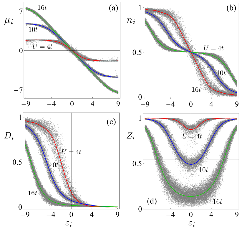
Figure 1: Summary of the GA solution for the AH model on a $30\times 30$ square lattice. The panels show the scatter diagram of (a) local energy correction $\mu_{i}$, (b) site electron density $n_{i}$, (c) probability of double occupation $D_{i}=d_{i}^{2}$, and (d) local quasi-particle weight $Z_{i}=\mathcal{R}_{i}^{2}$ versus the random site energy $\varepsilon_{i}$. The data points were obtained from calculations with random strength $W/t=6,10,14,18$ and three different $U=4t$, $10t$, and $16t$. The smooths curves showing the underlying overall trend for a given $U$ were obtained using polynomial regression with up to 14th-order polynomials. The red, blue, and green curves correspond to $U=4t$, $10t$, and $16t$, respectively.

Using the above GA solver on a $L=30$ square lattice, large datasets were generated with various disorder strengths $W/t=6,10,14,18$ and Hubbard parameters $U/t=2,4,\cdots,16$. The scatter plots in Fig. 1 show the various local quantities versus the random site energy $\varepsilon_{i}$ obtained from the GA solution with three different values of Hubbard repulsion. The local quantities are the site Lagrangian multiplier $\mu_{i}$, the local electron density $n_{i}$, the double occupation probability $D_{i}=d_{i}^{2}$, and the local quasi-particle weight $Z_{i}=\mathcal{R}_{i}^{2}$. Interestingly, for a given $U$, the data points cluster around a smooth curve, indicating an underlying continuous trend. More quantitatively, we used polynomial regression to determine the overall dependence of the local quantities on the site energy $\varepsilon_{i}$; see the solid curves in Fig. 1.

Extensive studies on the statistics of electron correlation in 2D AH model have been carried out using SB or real-space DMFT methods tanaskovic03 ; andrade09 ; andrade10 . One interesting phenomenon is the screening of the impurity potential due to electron correlations, especially close to the metal-insulator transition. Our result shown in Fig. 1(a) clearly demonstrates this trend. Indeed, from Eq. (3), one can define a renormalized site potential as $\tilde{\varepsilon}_{i}=\varepsilon_{i}+\mu_{i}$. The anti-correlation between $\mu_{i}$ and $\varepsilon_{i}$ thus results in a reduced effective site potential. Moreover, the local density $n_{i}$ exhibits a more homogeneous distribution in the vicinity of Fermi energy with increasing $U$; see Fig. 1(b).

The overall behavior of local quasi-particle weight versus $\varepsilon$ is consistent with the result obtained from TMT-DMFT using SB method as the impurity solver aguiar09 . As shown in Fig. 1(d), electrons at large $|\varepsilon_{i}|$ get less renormalization, i.e. retain a larger $Z_{i}$, compared with those close to the Fermi energy ($\varepsilon\sim 0$). Moreover, the difference between large and small $Z_{i}$ increases as one approaches the Mott transition boundary. This behavior also indicates a strong spatial inhomogeneity. While electrons in some regions become localized magnetic moments characterized by a vanishing $Z_{i}$, electrons in other regions undergo Anderson localization transition and maintains a large value of $Z_{i}$.

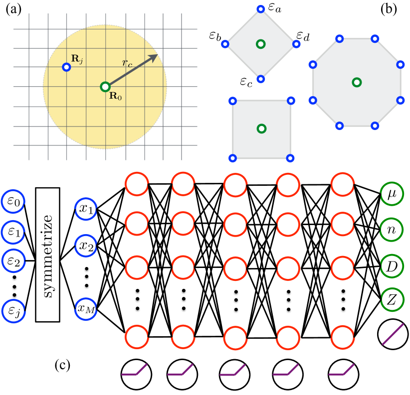
Figure 2: (a) Schematic showing the target site at $\mathbf{R}_{0}$ on the square lattice. Random potentials $\varepsilon_{j}$ of neighbors up to some cutoff radius $r_{c}$ are used as input to the neural network (NN). (b) Basic invariant subgroups of neighbors include two types of squares and a octagons. (c) Architecture of the fully-connected NN for the disordered correlated systems. For input, we use all the random-distributed on-site energies in the certain circle. ReLU activation function is used in the 5 hidden-feature extraction layers with $512\times 256\times 256\times 128\times 64$ nodes. The linear activation function is used to predict local quantities including $\mu$, $n$, $D$, and $Z$.

In order to capture the spatial site-to-site fluctuations of electron correlation, we next employ deep-learning techniques to predict the local electronic properties of the AH model. More specifically, our goal is to predict local quantities $\mu$, $n$, $D$, and $Z$ at a randomly picked site, say site-0, with the site potentials $\varepsilon_{j}$ in its neighborhood within a cutoff radius $r_{c}$ as the input; see Fig. 2(a). This, of course, is based on the assumption of locality which implies that correlation functions decay strongly with the distance. In general, the single-particle density matrix exhibits an exponential and a power decay for insulators and metals, respectively. The localization of electron wavefunctions due to disorder also enhances the decay of correlation functions, especially in 2D. To quantify this locality approximation, we have repeated our ML training with various $r_{c}$, and have verified that the predictions of the NNs are not sensitive to the cutoff radius. The results presented below were obtained by including up to 14th nearest neighbors with a total of 89 sites within the cutoff.

A proper representation of the site energies $\varepsilon_{j}$ is crucial in order to provide a description of the neighborhood that is invariant under fundamental transformations of the lattice symmetry. To this end, we first decompose all $\varepsilon_{j}$ into irreducible representations (irrep) of point group $D_{4}$, which is the site symmetry group of a square lattice. The neighboring sites can be classified into three different invariant sub-sets, as shown in Fig. 2(b). Decomposition of these sub-sets into the corresponding irreps is straightforward. Taking the square as an example, there are three irreps: $x_{A_{1}}=\varepsilon_{a}+\varepsilon_{b}+\varepsilon_{c}+\varepsilon_{d}$, $x_{B_{1}}=\varepsilon_{a}-\varepsilon_{b}+\varepsilon_{c}-\varepsilon_{d}$, and $\mathbf{x}_{E}=(\varepsilon_{a}-\varepsilon_{c},\varepsilon_{b}-\varepsilon_{d})$. The amplitudes of each irrep and their relative phases are then used as the input for the NN. For example, consider all doublet irreps: $\mathbf{x}_{m}$ with $m=1,2,\cdots,M$, where $M$ is the total number. The amplitudes $|\mathbf{x}_{m}|$, and relative angle $\cos\theta_{mn}=\mathbf{x}_{m}\cdot\mathbf{x}_{n}/|\mathbf{x}_{m}|\,|\mathbf{x}_{n}|$ are invariant under symmetry operations. We note that this descriptor of the site environment is similar to the atom-centered symmetry functions used in ML potentials for quantum molecular dynamics simulations behler07 ; botu15 .

We design a fully-connected neural network (NN) with 5 hidden layers consisting of $n=512\times 256\times 256\times 128\times 64$ rectified linear units (ReLU) neurons nair10 . The input layer is the symmetrized neighborhood $\varepsilon$ as discussed above. The NN performs a sequence of transformations on the input that are illustrated in Fig. 2(c). In the $m$-th layer, the $n$-th neuron processes the activation $\mathbf{a}^{(m-1)}$ from $(m-1)$-th layer through independent weights and biases $\mathbf{w}^{(m-1)}\mathbf{a}^{(m-1)}+\mathbf{b}^{(m-1)}$. After the ReLU functions, the outcome is fed forward to be processed by the output neuron with linear activation function. Importantly, here we adopt the multi-task ML technique caruana97 that forces the NN to learn multiple local electron properties simultaneously. The additional constraints coming from the multi-task setup helps the search for the true ML model because of the smaller set of models that can fit all properties simultaneously.

We use mean absolute error (MAE) as the cost function with the L2 regularization ng04 to avoid overfitting and a minimum batch size of 100. We use randomly mixed 900000 data samples as the training set and perform a 5-fold cross-validation during the training. The Glorot uniform initializer glorot10 and Adam optimizer kingma14 with learning rate of 0.00001 is applied for training process. Once the training process is successful, the trained neural network can rapidly predict the 237600 test data samples. Fig. 3 compares the ML prediction with the GA solutions for all accumulated configurations, i.e. those used in the training phase and the remaining configurations used for validation. For all four local quantities, the NN gives rather good predictions as attested by the small MAE, which is of the order of less than one percent of the mean values for all quantities.

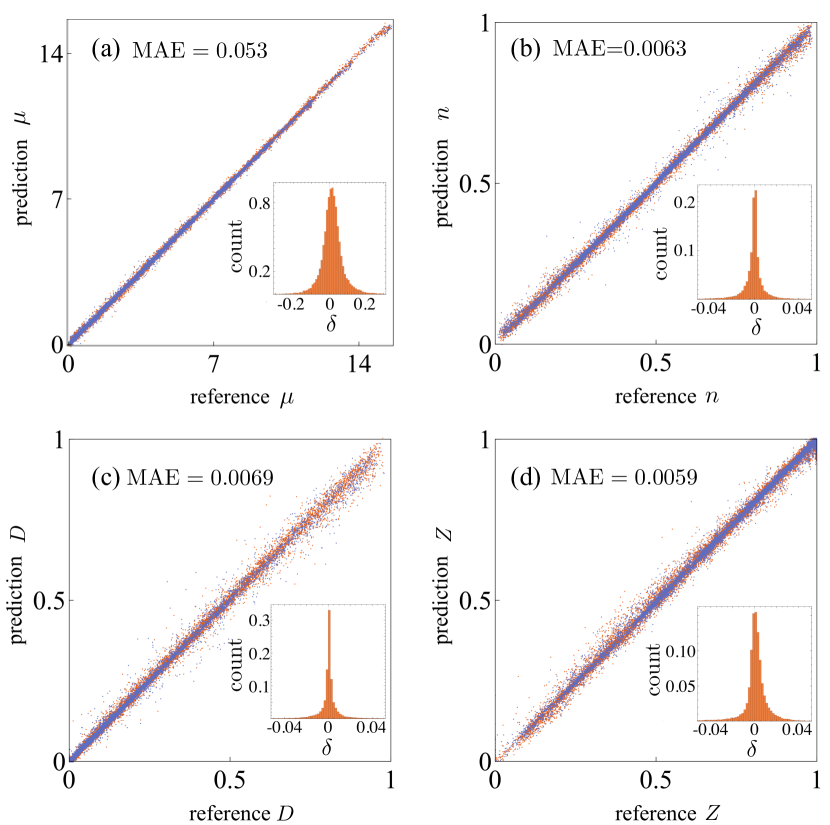
Figure 3: Comparison of the ML predictions with references obtained from the GA solvers, for (a) the local potential renormalization $\mu_{i}$, (b) site electron density $n_{i}$, (c) probability of double occupation $D_{i}$, and (d) local quasi-particle weight $Z_{i}$. The blue and orange data points denote predictions for training and test datasets, respectively. The insets show the normalized count of the error $\delta$ defined as the difference between prediction and reference values.

Discussion and Outlook. To summarize, we have introduced a ML model for predicting local electron correlation of Anderson-Hubbard Hamiltonian based on training a deep multi-task NN in configuration space. In order to describe the spatial inhomogeneity of the electronic structure, we use the real-space Gutzwiller method to numerically solve the AH model on a square lattice. Using the disorder potential in the neighborhood as the input, our ML trained NN is able to predict local electron properties such as double-occupancy and quasi-particle weight. Interesting phenomena such as the correlation induced screening of disorder potential and local Mott transition can be accurately predicted by our ML model. Our work provides a proof of principle study showing that deep NNs can serve as an efficient many-body problem solver for strongly correlated systems. For example, instead of the Gutzwiller solutions, one can train the NNs with data-sets obtained from the real-space DMFT or the VMC methods for the AH model. Although more computational effort is required to generate the training data, more accurate prediction can be achieved with the resultant NN model.

As discussed above, a primary motivation for ML trained NN is to bypass the expensive DFT calculation that is required in simulations such as ab initio molecular dynamics. Similarly, our proposed ML model as an efficient GA solver also has direct application for the molecular dynamics simulations of so-called Holstein-Hubbard model holstein59 ; pradhan15 ; disante17 , in which the site potential $\varepsilon_{i}=-gX_{i}$ is related to the amplitude of local phonon mode $X_{i}$, here $g$ is the electron-phonon coupling constant. In such simulations pradhan15 , forces acting on the local elastic modes are proportional to the local electron density $F_{i}=g\,n_{i}$, which can be efficiently computed using the trained NN. Another related application is to the recently proposed Gutzwiller molecular dynamics (GMD) chern17 . The atomic forces in this method are computed from the optimized Gutzwiller many-electron wavefunction at every time step. Contrary to DFT-based molecular dynamics, GMD simulations allow one to investigate the effects of electron correlation on atomic structural dynamics chern17 . Our work shows that ML techniques can be applied to develop a NN that efficiently emulates a GA solver. Preliminary results maro18 indeed show that ML is a promising approach for such applications.

Acknowledgment. We thank Kipton Barros for useful discussions on ML methods. G.W.C. thanks Vladmir Dobrosavljević for insightful discussions on slave-boson and Gutzwiller methods for disordered Hubbard models. P.Z. and G.W.C. are partially supported by the Center for Materials Theory as a part of the Computational Materials Science (CMS) program, funded by the US Department of Energy, Office of Science, Basic Energy Sciences, Materials Sciences and Engineering Division. J. Ma, Y. Tan and A.W.G. thank support from NSF-DMREF 1235230. The authors also acknowledge Advanced Research Computing Services at the University of Virginia for providing technical support that has contributed to the results in this paper.

References

- (1) T. M. Mitchell, Machine Learning (McGraw Hill, New York, 1997).
- (2) B. Schölkopf and A. J. Smola, Learning with Kernels (MIT, Cambridge, 2002).
- (3) M. Nielsen, Neural Networks and Deep Learning (Determination Press, 2015).
- (4) R. Duda, P. Hart, D. Stork, Pattern Classification, 2nd Ed. (Wiley, New York, 2001).
- (5) C. Bishop, Pattern Recognition and Machine Learning (Springer, Berlin, 2006).
- (6) B. G. Sumpter and D. W. Noid, On the design, analysis, and characterization of materials using computational neural networks, Annu. Rev. Mater. Sci. 26, 223 (1996).
- (7) S. V. Kalinin, B. G. Sumpter, and R. K. Archibald, Big-deep-smart data in imaging for guiding materials design, Nat. Mater. 14, 973 (2015).
- (8) P. V. Balachandran, B. Kowalski, A. Sehirlioglu, and T. Lookman, Experimental search for high-temperature ferroelectric perovskites guided by two-step machine learning, Nat. Commun. 9, 1668 (2018).
- (9) W. F. Reinhart, A. W. Long, M. P. Howard, A. L. Ferguson, and A. Z. Panagiotopoulos, Machine learning for autonomous crystal structure identification, Soft Matter 13, 4733 (2017).
- (10) C. Dietz, T. Kretz, and M. H. Thoma, Machine-learning approach for local classification of crystalline structures in multiphase systems, Phys. Rev. E 96, 011301(R) (2017).
- (11) N. Lubbers, T. Lookman, and K. Barros, Inferring low-dimensional microstructure representations using convolutional neural networks, Phys. Rev. E 96, 052111 (2017).
- (12) E. D. Cubuk, S. S. Schoenholz, J. M. Rieser, B. D. Malone, J. Rottler, D. J. Durian, E. Kaxiras, and A. J. Liu, Identifying Structural Flow Defects in Disordered Solids Using Machine-Learning Methods, Phys. Rev. Lett. 114, 108001 (2015).
- (13) S. S. Schoenholz, E. D. Cubuk, D. M. Sussman, E. Kaxiras, and A. J. Liu, A structural approach to relaxation in glassy liquids, Nat. Phys. 12, 469 (2016).
- (14) L. Wang, Discovering phase transitions with unsupervised learning, Phys. Rev. B 94, 195105 (2016).
- (15) J. Carrasquilla and R. G. Melko, Machine learning phases of matter, Nat. Phys. 13, 431 (2017).
- (16) S. J. Wetzel, Unsupervised learning of phase transitions: From principal component analysis to variational autoencoders, Phys. Rev. E 96, 022140 (2017).
- (17) W. Hu, R. R. P. Singh, and R. T. Scalettar, Discovering phases, phase transitions, and crossovers through unsupervised machine learning: A critical examination, Phys. Rev. E 95, 062122 (2017).
- (18) K. Ch’ng, J. Carrasquilla, R. G. Melko, and E. Khatami, Machine Learning Phases of Strongly Correlated Fermions, Phys. Rev. X 7, 031038 (2017).
- (19) P. Broecker, J. Carrasquilla, R. G. Melko, and S. Trebst, Machine learning quantum phases of matter beyond the fermion sign problem, Sci. Rep. 7, 8823 (2017).
- (20) Y. Zhang and E.-A. Kim, Quantum Loop Topography for Machine Learning, Phys. Rev. Lett. 118, 216401 (2017).
- (21) F. Schindler, N. Regnault, and Titus Neupert, Probing many-body localization with neural networks, Phys. Rev. B 95, 245134 (2017).
- (22) G. Torlai and R. G. Melko, Learning thermodynamics with Boltzmann machines, Phys. Rev. B 94, 165134 (2016).
- (23) G. Carleo and M. Troyer, Solving the quantum many-body problem with artificial neural networks, Science 355, 602 (2017).
- (24) D.-L. Deng, X. Li, and S. Das Sarma, Quantum Entanglement in Neural Network States, Phys. Rev. X 7, 021021 (2017).
- (25) F. Brockherde, L. Li, K. Burke, and K.-R. Müller, Bypassing the Kohn-Sham equations with machine learning, Nature Commun. 8, 872 (2017).
- (26) J. C. Snyder, M. Rupp, K. Hansen, K.-R. Müller, and K. Burke, “Finding Density Functionals with Machine Learning,” Phys. Rev. Lett. 108, 253002 (2012).
- (27) J. C. Snyder, M. Rupp, K. Hansen, L. Blooston, K.-R. Müller, and K. Burke, Orbital-free bond breaking via machine learning, J. Chem. Phys. 139, 224104 (2013).
- (28) L. Li, J. C. Snyder, I. M. Pelaschier, J. Huang, U.-N. Niranjan, P. Duncan, M. Rupp, K.-R. Müller, K. Burke, Understanding machine-learned density functionals, Int. J. Quantum Chem. 116, 819 (2016).
- (29) K. Yao and J. Parkhill, Kinetic energy of hydrocarbons as a function of electron density and convolutional neural networks, J. Chem. THeory Comput. 12, 1139 (2016).
- (30) L. Li, T. E. Baker, S. R. White, and K. Burke, Pure density functional for strong correlation and the thermodynamic limit from machine learning, Phys. Rev. B 94, 245129 (2016).
- (31) K. T. Schütt, F. Arbabzadah, S. Chmiela, K. R. Müller, and A. Tkatchenko, Quantum-chemical insights from deep tensor neural networks, Nature Commun. 8, 13890 (2017).
- (32) M. Rupp, A. Tkatchenko, K.-R. Müller, and O. A. von Lilienfeld, Fast and Accurate Modeling of Molecular Atomization Energies with Machine Learning, Phys. Rev. Lett. 108, 058301 (2012).
- (33) K. Hansen, G. Montavon, F. Biegler, S. Fazli, M. Rupp, M. Scheffler, O. A. von Lilienfeld, A. Tkatchenko, and K. B. Müller, Assessment and Validation of Machine Learning Methods for Predicting Molecular Atomization Energies, J. Chem. Theory Comput. 9, 3404 (2013).
- (34) J. Behler and M. Parrinello, Generalized Neural-Network Representation of High-Dimensional Potential-Energy Surfaces, Phys. Rev. Lett. 98, 146401 (2007).
- (35) A. P. Bartók, M. C. Payne, R. Kondor, G. Csányi, Gaussian Approximation Potentials: The Accuracy of Quantum Mechanics, without the Electrons, Phys. Rev. Lett. 104, 136403 (2010).
- (36) Z. Li, J. R. Kermode, and A. De Vita, Molecular Dynamics with On-the-Fly Machine Learning of Quantum-Mechanical Forces, Phys. Rev. Lett. 114, 096405 (2015).
- (37) V. Botu and R. Ramprasad, Learing scheme to predict atomic forces and accelerate materials simulations, Phys. Rev. B 92, 094306 (2015).
- (38) S. Chmiela, A. Tkatchenko, H. E. Sauceda, I. Poltavsky, K. T. Schütt, and K.-R. Müller, Machine learning of accurate energy-conserving molecular force fields, Sci. Adv. 3, e1603015 (2017).
- (39) L.-F. Arsenault, A. Lopez-Bezanilla, O. A. von Lilienfeld, and A. J. Millis, Machine learning for many-body physics: The case of the Anderson impurity model, Phys. Rev. B 90, 155136 (2014).
- (40) J. Liu, Y. Qi, Z. Y. Meng, and L. Fu, Self-learning Monte Carlo method, Phys. Rev. B 95, 041101(R) (2017).
- (41) X. Y. Xu, Y. Qi, J. Liu, L. Fu, and Z. Y. Meng, Self-learning quantum Monte Carlo method in interacting fermion systems, Phys. Rev. B 96, 041119(R) (2017).
- (42) L. Huang and L. Wang, Accelerated Monte Carlo simulations with restricted Boltzmann machines, Phys. Rev. B 95, 035105 (2017).
- (43) D. Heidarian and N. Trivedi, Inhomogeneous Metallic Phase in a Disordered Mott Insulator in Two Dimensions, Phys. Rev. Lett. 93, 126401 (2004).
- (44) H. Shinaoka and M. Imada, Single-Particle Excitations under Coexisting Electron Correlation and Disorder: A Numerical Study of the Anderson-Hubbard Model, J. Phys. Soc. Jpn. 78, 094708 (2009).
- (45) M. Ulmke, V. Janis, and D. Vollhardt, Anderson-Hubbard model in infinite dimensions, Phys. Rev. B 51, 10411 (1995).
- (46) M. Ulmke, R. T. Scalettar, Magnetic correlations in the two-dimensional Anderson-Hubbard model, Phys. Rev. B 55, 4149 (1997).
- (47) M. E. Pezzoli, F. Becca, M. Fabrizio, and G. Santoro, Local moments and magnetic order in the two-dimensional Anderson-Mott transition, Phys. Rev. B 79, 033111 (2009).
- (48) M. E. Pezzoli and F. Becca, Ground-state properties of the disordered Hubbard model in two dimensions, Phys. Rev. B 81, 075106 (2010).
- (49) V. Dobrosavljević and G. Kotliar, Mean Field Theory of the Mott-Anderson Transition, Phys. Rev. Lett. 78, 3943 (1997).
- (50) V. Dobrosavljević, D. Tanasković, and A. A. Pastor, Glassy Behavior of Electrons Near Metal-Insulator Transitions, Phys. Rev. Lett. 90, 016402 (2003).
- (51) K. Byczuk, W. Hofstetter, D. Vollhardt, Mott-Hubbard Transition versus Anderson Localization in Correlated Electron Systems with Disorder, Phys. Rev. Lett. 94, 056404 (2005).
- (52) M. C. O. Aguiar, V. Dobrosavljević, E. Abrahams, G. Kotliar, Critical Behavior at the Mott-Anderson Transition: A Typical-Medium Theory Perspective, Phys. Rev. Lett. 102, 156402 (2009).
- (53) A. Georges, G. Kotliar, W. Krauth, and M. J. Rozenberg, Dynamical mean-field theory of strongly correlated fermion systems and the limit of infinite dimensions, Rev. Mod. Phys. 68, 13 (1996).
- (54) V. Dobrosavljević, A. A. Pastor, and B. K. Nikolić, Typical medium theory of Anderson localization: A local order parameter approach to strong-disorder effects, Europhys. Lett. 62, 76 (2003).
- (55) D. Tanasković, V. Dobrosavljević, E. Abrahams, and G. Kotliar, Disorder Screening in Strongly Correlated Systems, Phys. Rev. Lett. 91, 066603 (2003).
- (56) E. C. Andrade, E. Miranda, and V. Dobrosavljević, Electronic Griffiths Phase of the Mott transition, Phys. Rev. Lett. 102, 206403 (2009).
- (57) E. C. Andrade, E. Miranda, and V. Dobrosavljević, Quantum Ripples in Strongly Correlated Metals, Phys. Rev. Lett. 104, 236401 (2010).
- (58) M. C. Gutzwiller, Effect of Correlation on the Ferromagnetism of Transition Metals, Phys. Rev. Lett. 10, 159 (1963).
- (59) G. Kotliar and A. E. Ruckenstein, New Functional Integral Approach to Strongly Correlated Fermi Systems: The Gutzwiller Approximation as a Saddle Point, Phys. Rev. Lett. 57, 1362 (1986).
- (60) N. Lanatá, H. U. R. Strand, Xi Dai, and B. Hellsing, Efficient implementation of the Gutzwiller variational method, Phys. Rev. B 85, 035133 (2012).
- (61) N. Lanatá, Y.-Xin Yao, C.-Z. Wang, K.-M. Ho, and G. Kotliar, Phase Diagram and Electronic Structure of Praseodymium and Plutonium, Phys. Rev. X 5, 011008 (2015).
- (62) V. Nair and G. E. Hinton, in Proceedings of the 27th International Conference on International Conference on Machine Learning, ICML’10 (Omnipress, USA, 2010) pp. 807-814.
- (63) R. Caruana, Multitask Learning, Mach. Learn. 28, 41 (1997).
- (64) A. Y. Ng, in Proceedings of the Twenty-first International Conference on Machine Learning, ICML’04 (ACM, New York, NY, USA, 2004) pp. 78
- (65) X. Glorot and Y. Bengio, in Proceedings of the Thir- teenth International Conference on Artificial Intelligence and Statistics, Proceedings of Machine Learning Research, Vol. 9, edited by Y. W. Teh and M. Titterington (PMLR, Chia Laguna Resort, Sardinia, Italy, 2010) pp. 249-256.
- (66) D. P. Kingma and J. Ba, arXiv:1412.6980 (2014).
- (67) T. Holstein, Studies of polaron motion: Part I. The molecular-crystal model, Ann. Phys. 8, 325 (1959).
- (68) S. Pradhan and G. V. Pai, Holstein-Hubbard model at half filling: A static auxiliary field study, Phys. Rev. B 92, 165124 (2015).
- (69) D. Di Sante, S. Fratini, V. Dobrosavljević, and S. Ciuchi, Disorder-Driven Metal-Insulator Transitions in Deformable Lattices, Phys. Rev. Lett. 118, 036602 (2017).
- (70) G.-W. Chern, K. Barros, C. D. Batista, J. D. Kress, G. Kotliar, Mott Transition in a Metallic Liquid: Gutzwiller Molecular Dynamics Simulations, Phys. Rev. Lett. 118, 226401 (2017).
- (71) H. Suwa, J. S. Smith, N. Lubbers, C. D. Batista, G.-W. Chern, K. Barros, Machine learning for molecular dynamics with strongly correlated electrons, in preparation.