Extreme Decoherence and Quantum Chaos

Abstract

We study the ultimate limits to the decoherence rate associated with dephasing processes. Fluctuating chaotic quantum systems are shown to exhibit extreme decoherence, with a rate that scales exponentially with the particle number, thus exceeding the polynomial dependence of systems with fluctuating $k$-body interactions. Our findings suggest the use of quantum chaotic systems as a natural test-bed for spontaneous wave function collapse models. We further discuss the implications on the decoherence of AdS/CFT black holes resulting from the unitarity loss associated with energy dephasing.

Decoherence is a ubiquitous phenomenon in nature, that is responsible for the emergence of classical behavior from the quantum substrate Rev03 ; Rev05 ; Book-Decoherence . Different sources of decoherence can be identified. Decoherence is most commonly attributed to the interaction between the system and its surrounding environment. However, it can also arise from the presence of random fluctuations in the system evolution. These can have an intrinsic quantum origin, as in the case of continuously monitored systems, or be associated with classical sources of noise, as those described by fluctuating Hamiltonians. In each case the dynamics becomes stochastic, and upon averaging over realizations of the noise processes, decoherence manifests itself in an ensemble perspective. This scenario has important applications in quantum optics Milburn98 , quantum simulations Rev12 ; Rev14 ; Dutta2016 ; Chenu2017 , quantum sensing sensing , and collapse models Bassi13 . In addition, the decoherence effect can also be independent of any direct interaction with an environment or noise fluctuations. In particular, a loss of unitarity can arise when quantum dynamics exhibits random phase changes on a short time scale Milburn91 , in the description of quantum evolution with realistic clocks of finite precision clock ; Diosi ; gravity , or as a result of gravitational effects Blencowe .

In general, decoherence increases with the system size Rev05 , making challenging quantum information and simulation tasks with complex quantum systems involving a large number of particles and degrees of freedom Rev08 ; Rev17 . For a complex quantum system that exhibits chaos, decoherence can be expected to be singular due to the enhanced sensitivity to initial conditions. Chaotic quantum systems can be described using random matrix Hamiltonians with appropriate symmetries Book-RMT ; Book-RMT1 . Originally, random matrix theory was introduced by Wigner to deal with the statistics of the spectra of heavy atomic nuclei Book-RMT ; Book-RMT1 ; Book-RMT2 ; Rev-nuclear ; Rev-nuclear2 . Recent progress includes applications to complex open quantum systems Mata11 ; Breuer11 ; Breuer13 , Majorana fermions Rev-F , many-body quantum chaos Kos18 ; Chan , work statistics in chaotic systems Chenu17 ; Chenu18 ; work , and information scrambling in black holes Preskill ; scramble ; Barbon ; Maldacena2016 ; Dyer17 ; Cotler1 ; delCampo17prd ; Cotler2 ; Vegh .

Understanding the interplay between quantum chaos and decoherence is a longstanding problem. Earlier studies of this subject are mainly focused on the effect of dissipation and decoherence on level statistics, and how to incorporate such effects into the study of quantum systems that are chaotic in the classical limit Book-RMT1 ; Book-Chaos2 . Here, we pose the question as to what is the ultimate limit to the rate of decoherence of complex quantum systems. This issue is not only of relevance to fundamental and applied aspects of quantum science and technology, but has implications that extend to other fields, including black-hole physics. In this Letter, we introduce a decoherence rate that applies to arbitrary Markovian processes. Using it, we show that the dynamics of fluctuating chaotic quantum systems is extreme in that its rate scales exponentially with the number of particles $n$. Such scaling has no match in physical systems with $k$-body interactions, where the decoherence rate scales polynomially with $n$. In turn, this allows us to identify chaotic quantum systems described by random matrix theory as a natural test-bed for spontaneous wavefunction collapse models.

Decoherence rates.— A Markovian open quantum system is generally described by a master equation of the Lindblad form Lindblad ; Book-Open

$$\dot{\rho}_{t}=-\frac{i}{\hbar}\left[H,\rho_{t}\right]+\sum_{\mu}\gamma_{\mu}\left(V_{\mu}\rho_{t}V_{\mu}^{{\dagger}}-\frac{1}{2}\{V_{\mu}^{{\dagger}}V_{\mu},\rho_{t}\}\right),$$ (1)

where the Hamiltonian $H$ determines the unitary evolution of the system, the coupling constants $\gamma_{\mu}\geq 0$ are non-negative, and $V_{\mu}$ are the corresponding Lindblad operators.

In order to characterize how fast the system decoheres, we consider the purity $P_{t}:=\mathrm{{tr}\left(\rho_{t}^{2}\right)}$ of the state, which quantifies its degree of mixedness. An expression for the decoherence rate under Markovian evolution can be obtained from the short-time asymptotic behavior $P_{t}=$tr$\left(\rho_{0}^{2}\right)+2$tr$\left(\rho_{0}\dot{\rho}_{0}\right)t+\mathcal{O}(t^{2})\simeq P_{0}(1-Dt)$, from which we define the decoherence rate note

$$D:=-\frac{2\text{tr}\left(\rho_{0}\dot{\rho}_{0}\right)}{\text{tr}\left(\rho_{0}^{2}\right)}=\frac{2\sum_{\mu}\gamma_{\mu}\widetilde{\mathrm{cov}}_{\rho_{0}}(V_{\mu}^{{\dagger}},V_{\mu})}{\text{tr}\left(\rho_{0}^{2}\right)},$$ (2)

where $\widetilde{\mathrm{cov}}_{\rho_{0}}(X,Y):=\left\langle\rho_{0}XY\right\rangle_{\rho_{0}}-\left\langle X\rho_{0}Y\right\rangle_{\rho_{0}}$ is the modified covariance, with $\left\langle X\right\rangle_{\rho_{0}}:=$tr$\left(\rho_{0}X\right)$. Equation (2) depends only on the initial state and Lindblad operators, facilitating the analysis of decoherence in complex quantum systems without the need to solve the dynamical equations of motion. Equation (2) further extends Zurek’s seminal estimate of the decoherence time Rev03 , derived in the context of quantum Brownian motion, to arbitrary Markovian dynamics.

In what follows we shall be interested in Hermitian Lindblad operators $V_{\mu}$, when Eq. (1) can also be rewritten in a double-commutator form. The purity is then guaranteed to decrease monotonically with time, $\dot{P}_{t}<0$ for all $t\geq 0$ Lidar06 . In particular, we shall focus on $V_{\mu}$ described by random matrices as well as $k$-body interaction operators. Such instances of $V_{\mu}$ are natural in a wide variety of scenarios including the description of fluctuating Hamiltonian systems and collapse models, as described below.

Extreme decoherence rates with random-matrix Lindblad operators.— Statistical spectral properties of quantum chaotic systems can be conveniently described using ensembles of random matrix operators $\{X\}$ Book-RMT ; Book-RMT1 . Gaussian ensembles are associated with operators in which matrix elements are i.i.d. complex Gaussian variables. Gaussian ensembles can be classified in terms of the invariance of the joint eigenvalue density $\varrho(X)$ under similarity transforms, $\varrho(X)=\varrho(UXU^{-1})$. Prominent examples include orthogonal, unitary or symplectic matrices $U$ Book-RMT2 . When the dimension of the Hilbert space is large, properties such as the eigenvalue density become universal and are shared by the different ensembles.

We shall consider the decoherence under chaotic Lindblad operators $V_{\mu}$ sampled from the Gaussian Unitary Ensemble (GUE) with dimension $d$, i.e., $V_{\mu}\in$ GUE. To this end, we introduce a simplified GUE average of a function $f(X)$ ($X\in$ GUE) with Haar measure SM

$$\left\langle f(X)\right\rangle_{\mathrm{GUE}}:=\int\prod_{k=1}^{d}\mathrm{d}x_{k}\varrho_{\mathrm{GUE}}(x_{1},\dots,x_{d})\left\langle f(X)\right\rangle_{\text{{Haar}}},$$ (3)

where $\varrho_{\mathrm{GUE}}(x_{1},\dots,x_{d})$ is the $d$-point correlation function for the eigenvalues {$x_{k}$}_k=1,⋯,d of $X$, and $\left\langle f(X)\right\rangle_{\text{{Haar}}}:=\int_{\mathcal{U}(d)}f(UHU^{-1})\mathbf{d}\mu(U)$ denotes the Haar average over the unitary group $\mathcal{U}(d)$ with Haar measure $\mathbf{d}\mu(U)$ Book-Haar ; Haar ; Book-RMT3 ; Book-Tao . Without loss of generality, the initial state is assumed to be pure with $\rho_{0}=\left|\Psi_{0}\right\rangle\left\langle\Psi_{0}\right|$ (see SM for the mixed state case). As shown in SM , when the initial pure state $\rho_{0}$ is fixed and chosen independently of $V_{\mu}$, the decoherence rate with averaged over GUE reads

$$D_{\mathrm{GUE}}=\frac{2d}{d+1}\sum_{\mu}\gamma_{\mu}\langle\mathrm{var}_{\rho_{\beta=0}}(V_{\mu})\rangle_{\mathrm{GUE}}=\frac{\Gamma d^{2}}{d+1},$$ (4)

where $\mathrm{var}_{{}_{\rho}}(X):=\left\langle X^{2}\right\rangle_{\rho}-\left\langle X\right\rangle_{\rho}^{2}$ denotes the variance of $X$ in the state $\rho$, $\rho_{\beta=0}=\mathds{1}_{d}/d$ is the thermal state at infinite temperature, and $\Gamma:=\sum_{\mu}\gamma_{\mu}$. Note that information regarding the initial state is lost with the Haar average in the first equality, as the variance is expressed only in terms of the thermal state at infinite temperature. In Eq. (4), the second equality follows from using the corresponding correlation function $\varrho_{\mathrm{GUE}}$ of GUE. We note that the scaling of the decoherence rate in Eq. (4) stems from the dependence of the density of states on the Hilbert space dimension in systems described by random matrices. In particular, it is independent of other spectral signatures of chaos, such as the level spacing distribution Book-RMT ; Book-RMT1 .

For simplicity, we consider a single chaotic operator $V$ with rate $\gamma$. Assuming for the sake of illustration that the system is composed of $n$ qubits with a Hilbert space dimension $d=2^{n}$, the corresponding decoherence rate for chaotic operators becomes extremely fast, with $D_{\mathrm{GUE}}=\gamma 2^{2n}/(2^{n}+1)\simeq\gamma 2^{n}$. Decoherence is then exponentially faster than in the case of $k$-body Lindblad operators, except for extremely non-local interactions, with $k\gtrsim\mathcal{O}(n)$. To show this, consider the general case of a $k$-body Lindblad operator of the form

$$V=\epsilon\sum_{l_{1}<\cdots<l_{k}}^{n}\Lambda_{l_{1}<\cdots<l_{k}},$$ (5)

where $\epsilon$ is a dimensionless positive constant to be determined by comparison with GUE, as discussed below. The variance is bounded by $\mathrm{var}_{{}_{\rho_{0}}}(V)\leq\left\|V\right\|^{2}$, where $\left\|X\right\|:=x_{M}$ is the spectral norm and $x_{M}$ is the maximum eigenvalue of $\sqrt{X^{{\dagger}}X}$ SM . The spectral norm of $V$ in Eq. (5) is given by

$$\left\|V\right\|\leq\epsilon\sum_{l_{1}<\cdots<l_{k}}^{n}\left\|\Lambda_{l_{1}<\cdots<l_{k}}\right\|=\epsilon\left\|\Lambda_{l_{1}<\cdots<l_{k}}\right\|\binom{n}{k},$$ (6)

where $\binom{n}{k}:=\frac{n!}{k!(n-k)!}$ is the binomial coefficient. Therefore, the decoherence rate for the $k$-body case satisfies

$$D_{k-\mathrm{body}}\lesssim\frac{2\gamma\epsilon^{2}\left\|\Lambda_{l_{1}<\cdots<l_{k}}\right\|^{2}}{(k!)^{2}}n^{2k},$$ (7)

where we have assumed $k\ll n$. Said differently, the decoherence rate of the $k$-body system grows at most polynomially in $n$. For the sake of illustration, we consider an example in which the decoherence operator given by a $k$-body all-to-all long-range term $\Lambda_{l_{1}<\cdots<l_{k}}=\sigma_{l_{1}}^{z}\otimes\cdots\otimes\sigma_{l_{k}}^{z}\otimes\mathds{1}_{\delta\neq l_{1},\cdots,l_{k}}$, where $\sigma^{z}$ is the usual Pauli operator. As $\left\|\Lambda_{l_{1}<\cdots<l_{k}}\right\|\equiv 1$, we have $D_{k-\mathrm{body}}\lesssim 2\gamma\epsilon^{2}n^{2k}/(k!)^{2}$. In order to perform a direct comparison between GUE and $k$-body systems, we set $D_{\text{GUE}}(n_{0})=D_{k\text{-body}}(n_{0})$, where $n_{0}$ is an arbitrary starting reference point for the particle number, with which the parameter $\epsilon$ can be determined. Fig. 1 presents numerical calculations for $n_{0}=1$ and $\epsilon^{2}=2/3$ as an example, showing that the decoherence rate for random operators is larger than for $k$ -body ones as long as $k\lesssim[n/10+1]$ in this case. This implies that chaotic dephasing described by random matrix theory not only leads to decoherence in an extreme way, but also faster than the physical $k$-body quantum systems in high dimensional situations, which we illustrate in Fig. 1. We expand this discussion with a spin model of two-body random ensembles TBRE in the Supplemental Material SM .

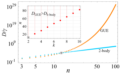
Figure 1: Extreme decoherence. Comparisson of the decoherence rates associated with fluctuating chaotic systems $D_{\mathrm{GUE}}$ and $k$-body systems $D_{k-\mathrm{body}}$, with $k=2$ as an example. Inset: The red dots represent the minimum particle number $n$ for which the decoherence rate in a chaotic system surpasses that of $k$-body system. The condition when $D_{\mathrm{GUE}}>$ $D_{k-\mathrm{body}}$ is $k\lesssim[n/10+1]$.

Decoherence rates of entangled states.— In what follows we illustrate extreme decoherence in an entangled state. For simplicity, we consider a thermal state of the form $\rho_{0}=e^{-\beta H}/Z(\beta)$, where the normalization constant is given by the partition function $Z(\beta):=\mathrm{tr}(e^{-\beta H})$, with inverse temperature $\beta=(k_{B}T)^{-1}$. This is a mixed state that can be purified by doubling the Hilbert space dimension and considering two identical copies of the system. The resulting entangled state is known as the thermofield double (TFD) state Book-TFD

$$\left|\Phi_{0}\right\rangle:=\frac{1}{\sqrt{Z(\beta)}}\sum_{k}e^{-\frac{\beta E_{k}}{2}}\left|k\right\rangle\left|k\right\rangle.$$ (8)

where $E_{k}$ ($\left|k\right\rangle$) are the corresponding eigenvalues (eigenvectors) of $H$. Tracing over any of the subsystems recovers the thermal state. TFD states are commonly used in finite-temperature field theory and have been widely studied in the context of holography, e.g., in connection to the entanglement between black holes Maldacena2013 , the butterfly effect  butterfly , and quantum source-channel codes code .

Here, we focus on sources of decoherence that act on the energy basis, as those arising in certain spontaneous wave function collapse models, that constitute stochastic modifications of quantum mechanics leading to localization in energy Gisin84 ; Percival94 ; SSE-PRD ; Bassi13 ; BG03 . An equivalent source of decoherence arises in the presence of fluctuating fields or coupling constants in the Hamiltonian Chenu2017 and random measurement Hamiltonians Korbicz17 . As already noted, decoherence in the energy eigenbasis arises as well if quantum dynamics at short time scales includes intrinsic uncertainties Milburn91 or when the time-evolution is described according to a realistic clock of finite precision; see clock ; gravity and SM .

Decoherence in the energy eigenbasis can generally be described in terms of fluctuating Hamiltonians. Assume now that each subsystem is perturbed by a single Gaussian real white noise $\xi_{t}$ Book-Stochastic , i.e., $H\rightarrow(1+\hbar\sqrt{\gamma_{L(R)}}\xi_{t}^{L(R)})H$ when $t>0$. Then, the total Hamiltonian is given by $\tilde{H}_{t}=H\otimes\mathds{1}+\mathds{1}\otimes H+\hbar\sqrt{\gamma}(\xi_{t}^{L}H\otimes\mathds{1}+\mathds{1}\otimes\xi_{t}^{R}H)$, where we assume independent noises $\xi_{t}^{L}\neq\xi_{t}^{R}$, with identical amplitudes $\gamma_{L}=\gamma_{R}=\gamma$ (here the tilde “$\sim$” is used to represent the global Hilbert space of the two copies). The dynamics of the system is governed by the Schrödinger equation $i\hbar\partial_{t}|\Psi_{t}^{\xi}\rangle=\tilde{H}_{t}|\Psi_{t}^{\xi}\rangle$, denoting $\xi:=\{\xi_{t}^{L},\xi_{t}^{R}\}$ for simplicity. Using Novikov’s theorem Novikov or Itô calculus SSE-PRD , one can show that the dynamics of the noise-averaged density matrix $\rho_{t}=\langle|\Psi_{t}^{\xi}\rangle\langle\Psi_{t}^{\xi}|\rangle_{\xi}$ is governed by the master equation (1), with Lindblad operators $\tilde{V}_{1}=H\otimes\mathds{1}$ and $\tilde{V}_{2}=\mathds{1}\otimes H$; see details in SM . The exact evolution of the density matrix reads SM ,

$$\rho_{t}=\frac{1}{Z(\beta)}\sum_{k,\ell}e^{-\frac{\beta}{2}E_{k\ell}^{+}-i\frac{2t}{\hbar}E_{k\ell}^{-}-\gamma t(E_{k\ell}^{-})^{2}}|k\rangle|k\rangle\langle\ell|\langle\ell|,$$ (9)

where $E_{k\ell}^{\pm}:=E_{k}\pm E_{\ell}$. The decay of the purity is thus given by

$$P_{t}=\sqrt{\frac{1}{8\pi\gamma t}}\int_{-\infty}^{\infty}e^{-\frac{y^{2}}{8\gamma t}}\left|\frac{Z(\beta-iy)}{Z(\beta)}\right|^{2}\mathrm{d}y,$$ (10)

in terms of the analytic continuation of the partition function. At long times, the purity approaches $P_{\infty}=Z(2\beta)/Z(\beta)^{2}$, which is the purity of a canonical thermal state at temperature $\beta$ and reduces to $1/d$ at infinite temperature ($\beta=0$). The corresponding decoherence rate can be immediately obtained from Eq. (2)

$$\tilde{D}=4\gamma\mathrm{var}_{\rho_{\beta}}(H)=4\gamma\frac{\mathrm{d}^{2}}{\mathrm{d}\beta^{2}}\ln\left[Z(\beta)\right],$$ (11)

where $Z(\beta)=\int\mathrm{d}E\varrho(E)e^{-\beta E}$, and $\varrho(E)$ is the spectral density of $H$.

Let us first consider $H$ modeled by a random matrix sampled from GUE Maldacena2016 ; Cotler1 . Given that the initial TFD state is defined in terms of the Hamiltonian $H$, some care is needed when performing the average in this case. In the following, we calculate the purity $\left\langle P_{t}\right\rangle_{\text{{GUE}}}$ shown in Fig. 2(a), and characterize the decoherence rate $\tilde{D}_{\text{{GUE}}}$. From Eq. (11), the latter is given by

$$\tilde{D}_{\text{{GUE}}}\doteq 4\gamma\frac{\mathrm{d}^{2}}{\mathrm{d}\beta^{2}}\ln[\left\langle Z(\beta)\right\rangle_{\text{{GUE}}}],$$ (12)

where “$\doteq$” indicates the use of the annealing approximation, that we show to be highly accurate in SM . For the average $\left\langle Z(\beta)\right\rangle_{\text{{GUE}}}=\int\mathrm{d}E\varrho_{\text{{GUE}}}(E)e^{-\beta E}$, using Wigner’s semicircle law in the limit of $d\gg 1$ one finds $\left\langle Z(\beta)\right\rangle_{\text{{GUE}}}=\sqrt{2d}\,\mathrm{I}_{1}(\sqrt{2d}\beta)/\beta$, where $\mathrm{I}_{n}(\cdot)$ is the modified Bessel function of first kind and order $n$ Book-Int . From Eq. (12), it then follows that SM

$$\tilde{D}_{\mathrm{GUE}}=8\gamma d\left[1-\frac{3}{\sqrt{2d}\beta}g(\sqrt{2d}\beta)-g(\sqrt{2d}\beta)^{2}\right],$$ (13)

with $g(x):=\mathrm{I}_{2}(x)/\mathrm{I}_{1}(x)$. The decoherence rate is depicted as a function of particle number under different $\beta$ in Fig. 2(b). Specifically, as a function of the temperature, the decoherence rate in Eq. (S59) simplifies to

$${\tilde{D}}_{\text{{GUE}}}\simeq\left\{\begin{array}[]{ll}2\gamma d,&(\beta\ll\beta_{c}),\\ \frac{6\gamma}{\beta^{2}},&(\beta\gg\beta_{c}),\end{array}\right.$$ (14)

where $\beta_{c}:=\sqrt{3/d}$. In the high temperature limit, when $\beta\ll$ $\beta_{c}$ the decoherence time reduces to ${\tilde{D}}_{\text{{GUE}}}\simeq 2\gamma d$ in agreement with Eq. (4). When $\beta\gg$ $\beta_{c}$, ${\tilde{D}}_{\text{{GUE}}}$ asymptotically approaches to $6\gamma/\beta^{2},$ proportional to the temperature square, i.e., at low temperature decoherence is highly suppressed, as shown in Fig. 2(c).

Next we illustrate the extent to which the decoherence of fluctuating quantum chaotic Hamiltonians is extreme and faster than physical systems with 2-body interactions. To this end, we compare the decoherence rate of a high-temperature TFD state of a chaotic quantum system with that of a spin Hamiltonian with all-to-all long-range $2$-body interactions. In particular, we consider Lipkin-Meshkov-Glick model with zero external magnetic field, with a Hamiltonian $H_{0}=\epsilon\sum_{l<m}^{n}\sigma_{l}^{z}\otimes\sigma_{m}^{z}$ ($n\geq 2$) that is amenable to quantum simulation XPeng ; Rey . For the latter, in the high temperature limit $\tilde{D}_{\text{{2-body}}}|_{\beta\ll\beta_{c}}\simeq 2\gamma n(n-1)$, which has a polynomial dependence on $n$. In spite of the all-to-all pairwise interactions, the rate is slower than that in the GUE case, that is characterized by extreme decoherence ($\tilde{D}_{\text{{GUE}}}|_{\beta\ll\beta_{c}}\simeq 2\gamma 2^{n}$ for qubits).

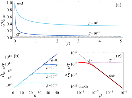
Figure 2: Decoherence of a thermofield double state. (a) Purity $\left\langle P_{t}\right\rangle_{\text{{GUE}}}$ as a function of $\gamma t$ with different temperatures $\beta$. The numerical average is performed over 1000 realizations of GUE with $n=5$. (b) The decoherence rates for GUE $\tilde{D}_{\mathrm{GUE}}/\gamma$ versus the particle (treated as qubits) number $n$ for different temperatures $\beta$. With the increase in the Hilbert space dimension, $\tilde{D}_{\mathrm{GUE}}/\gamma$ saturates at $6/\beta^{2}$. (c) The decoherence rates (red solid curve) for GUE $\tilde{D}_{\mathrm{GUE}}/\gamma$ as a function of $\beta$ with $n=50$. The asymptotic expressions for $\tilde{D}_{\mathrm{GUE}}/\gamma=2^{n+1}$ under $\beta\ll\beta_{c}:=\sqrt{3/2^{n}}$ (purple dotted-dashed line) and $\tilde{D}_{\mathrm{GUE}}/\gamma=6/\beta^{2}$ under $\beta\gg\beta_{c}$ (black dashed line) are also shown.

Decohrence of AdS/CFT black holes.— The decoherence of black holes induced by Hawking radiation has been widely studied Rev-BH ; Demers ; Arrasmith . The preceding analysis can be applied to the decoherence of eternal AdS-Schwarzschild black holes. According to the AdS/CFT correspondence, quantum gravity in an asymptotically anti-de Sitter (AdS) space-time is dual to a non-gravitational conformal field theory (CFT) on a lower dimensional space-time AdS ; Rev-BH ; Mark . Here, we consider a thermofield double (TFD) state of two non-interacting copies of CFT TFD ; Maldacena2003 ; rev . This can be interpreted as two entangled black holes in disconnected space, with common time. EPR correlations in the TFD state make the geometry of the two black holes connected by an Einstein-Rosen (ER) bridge. Said differently, one possible interpretation of the TFD state is that it is dual to two eternal AdS-Schwarzschild black holes in disconnected spaces with a common time Maldacena2013 . In this case, the total Hamiltonian is simply the sum of the two CFT Hamiltonians $\tilde{H}=H\otimes\mathds{1}+\mathds{1}\otimes H$ in Hilbert spaces $\mathcal{H}\otimes\mathcal{H}$ Maldacena2013 . According to the EPR=ER conjecture Maldacena2013 ; EREPR1 ; EREPR2 , the presence of entanglement and EPR correlations is associated with a geometry of an Einstein-Rosen bridge describing the entangled black holes. Unitarity loss associated with energy dephasing leads to the decay of of quantum correlations. The resulting decoherence of the TFD state results in the closing of the Einstein-Rosen bridge. While certain aspects of the late-time behavior of AdS/CFT black holes are captured by random matrix theory Cotler1 , decoherence is however not extreme in this context. Indeed, the decoherence rate can be written in terms of the heat capacity $C$ of the CFT as $\tilde{D}=4\gamma C/(k_{B}\beta^{2})$. The latter is proportional to the the entropy of the black hole $S$, which scales with the number of degrees of freedom $n$ PR15 .

Discussion and Conclusions.— We have introduced a decoherence rate for arbitrary Markovian processes and used it to demonstrate that fluctuating chaotic systems described by random matrix theory exhibit extreme decoherence. The latter is characterized by a rate that grows exponentially with the particle number, thus surpassing the dynamics of non-chaotic $k$-body Hamiltonians. This conclusion holds generally for any source of decoherence acting on the energy eigenbasis. Our findings suggest that chaotic quantum systems provide an ideal test-bed to explore deviations from quantum mechanics, such as those predicted by spontaneous wave function collapse models. This identification motivates the extension of current experimental efforts Bassi16 ; Bassi17 to probe decoherence in the energy basis. We have also applied our analysis to the fate of black holes under unitarity loss in the context of AdS/CFT and shown that the decoherence is not extreme in this context, in spite of the known random-matrix behavior at long times.

A surge of activity has recently been devoted to probing aspects of many-body quantum chaos and related models in a variety of platforms including trapped ions Rey ; ions2 , nuclear magnetic resonance systems Du ; Luo17 , ultracold atoms ultracold atom1 ; ultracold atom2 ; ultracold atom3 ; tocape , and superconducting qubits Laura17 . In particular, the generation of Haar-uniform random operations has been proposed in many-body systems driven by stochastic external pulses Banchi17 . We hope that the present work stimulates both theoretical and experimental research on the extreme decoherence rates in chaotic complex quantum systems, that is at reach with current technology.

Acknowledgements.—The authors are indebted to B. Swingle for clarifications on black hole decoherence. It is also a pleasure to thank F. J. Gómez-Ruiz, J. Molina-Vilaplana, J. Sonner and J. Maldacena for feedback on the manuscript. We acknowledge funding support by UMass Boston (project P20150000029279), the John Templeton Foundation, and the National Natural Science Foundation of China (Grant No. 11674238).

Supplemental Material–Extreme Decoherence: from Quantum Chaos to Black Holes

.1 A. Derivation of decoherence rate in GUE

.1.1 1. GUE average and Haar measure

The GUE average of function $f(X)$ ($X\in$GUE with dimension $d$), denoted as

$$\langle f(X)\rangle_{\mathrm{GUE}}:=\int f(X)\mathbf{d}\mu(X),$$ (S1)

is obtained for the ensemble probability measure

$$\mathbf{d}\mu(X):=Ce^{-\mathrm{{tr}(}X^{2}\mathrm{)}}\mathbf{d}X,\text{ with }\mathbf{d}X:=\prod_{j}\mathrm{d}X_{jj}\prod_{k<l}\mathrm{d}(\mathrm{Re}X_{kl})\,\mathrm{d}(\mathrm{Im}X_{kl}),$$ (S2)

where $C$ is a normalization constant, given in e.g. Ref. sBook-RMT , and $\mathbf{d}X$ is the flat Lebesgue measure on $d\times d$ Hermitian matrices $X$. Every $X\in$GUE can be diagonalized with a unitary operator $U$ [$U\in\mathcal{U}(d)$], i.e., $X=U\tilde{X}U^{-1}$, with $\tilde{X}_{jk}=x_{j}\delta_{jk}$. Thus,

$$\mathrm{d}X:=\left(\mathrm{d}X_{jk}\right)_{d\times d}=\mathrm{d}(U\tilde{X}U^{-1})=U\left[\mathrm{d}\tilde{X}+U^{-1}(\mathrm{d}U)\tilde{X}-\tilde{X}U^{-1}\mathrm{d}U\right]U^{-1},$$ (S3)

where $\mathrm{d}U:=(\mathrm{d}U_{jk})_{d\times d}$. The line element in the space of the entries of Hermitian matrices $X$ reads

$$\mathrm{d}s^{2}:=\text{tr}\left(\mathrm{d}X^{2}\right)=\sum_{j}(\mathrm{d}x_{j})^{2}-\sum_{k<l}(x_{k}-x_{l})^{2}\delta u_{kl}\delta u_{lk},$$ (S4)

where $\delta u_{kl}:=(U^{-1}\mathrm{d}U)_{kl}$. The flat Lebesgue measure $\mathbf{d}X$ can be induced from Eq. (S4) as (see, e.g., Ref. sBook-RMT2 )

$$\mathbf{d}X=\varepsilon\prod_{j}\mathrm{d}x_{j}|\Delta(x)|^{2}\mathbf{d}\mu(U),$$ (S5)

where $|\Delta(x)|^{2}:=\prod_{k<l}(x_{k}-x_{l})^{2}$ is the squared Vandermonde determinant, and $\mathbf{d}\mu(U)$ is the uniform probability (Haar) measure on the unitary group $\mathcal{U}(d)$ being normalized $\int_{\mathcal{U}(d)}\mathbf{d}\mu(U)=1$ with a constant $\varepsilon$. Using Eq. (S2) and Eq. (S5) together with Eq. (S1), the GUE average reads

$$\langle f(X)\rangle_{\mathrm{GUE}} = \int f(X)\varrho_{\text{{GUE}}}(x_{1},\dots,x_{d})\prod_{j}\mathrm{d}x_{j}\int_{\mathcal{U}(d)}\mathbf{d}\mu(U)$$ (S6)

$$= \int f(X)\varrho_{\text{{GUE}}}(x_{1},\dots,x_{d})\prod_{j}\mathrm{d}x_{j},$$

where $\varrho_{\text{{GUE}}}(x_{1},\dots,x_{d}):=C^{\prime}\exp(-\sum_{j}x_{j}^{2})|\Delta(x)|^{2}$ ($C^{\prime}=C\varepsilon$, given in e.g. Ref. sBook-RMT ) is the the $d$-point joint probability distribution of the eigenvalues, and the normalized condition of Haar measure has been employed in the second line of Eq. (S6). Specifically, Equation (S6) can be written as

$$\langle f(X)\rangle_{\mathrm{GUE}}=\int f(X)\varrho_{\mathrm{GUE}}(x)\mathrm{d}x,$$ (S7)

when we just consider the level density, i.e., $\varrho_{\mathrm{GUE}}(x)=\int\varrho_{\mathrm{GUE}}(x_{1},\dots,x_{d})\prod_{j=2}\mathrm{d}x_{j}$.

Since the probability measure $\mathbf{d}\mu(X)$ is invariant under the unitary conjugation of $X$ ($X\rightarrow UXU^{-1}$) sBook-Tao , we can employ the Haar measure to simplify the calculation. Equation (S6) can be rewritten as

$$\langle f(X)\rangle_{\mathrm{GUE}} = \int\varrho_{\mathrm{GUE}}(x_{1},\dots,x_{d})\left[\int_{\mathcal{U}(d)}f(UXU^{-1})\mathbf{d}\mu(U)\right]\prod_{j}\mathrm{d}x_{j}$$ (S8)

$$= \int\left\langle f(X)\right\rangle_{\mathrm{Haar}}\text{{D}}x,$$

where we have introduced D$x:=\varrho_{\mathrm{GUE}}(x_{1},\dots,x_{d})\prod_{j}\mathrm{d}x_{j}$, and the Haar average

$$\left\langle f(X)\right\rangle_{\mathrm{Haar}}:=\int_{\mathcal{U}(d)}f(UXU^{-1})\mathbf{d}\mu(U),$$ (S9)

in the second line for simplicity.

Note that as long as $\varrho_{\text{{GUE}}}(x_{1},\dots,x_{d})$ is known, the GUE average can be evaluated using Eq. (S6). However, the calculation can be greatly simplified with Eq. (S8) provided the moment function (Haar average) of the unitary group is given (see e.g., the following section).

.1.2 2. Proof of Eq. (4) in the main text

In this section, we give a proof of the following bound

$$D_{\text{{GUE}}}\leq\Gamma\frac{d^{2}}{d+1},$$ (S10)

where $\Gamma:=\sum_{\mu}\gamma_{\mu}$, and $d$ is the Hilbert space dimension of the system. The equality is achieved when the initial state is pure [i.e., Eq. (4) in the main text].

Proof.  In this work, we consider the chaotic decoherence channels, with Lindblad operators $\{V_{\mu}\}$ sampled from random the Gaussian unitary ensemble $(\mathrm{GUE})$. Therefore, $\{V_{\mu}\}$ are the Hermitian operators, and the decoherence rate [Eq. (2) in the main text] can be written as

$$D:=-\frac{2\text{tr}(\rho_{0}\dot{\rho}_{0})}{\text{tr}\left(\rho_{0}^{2}\right)}=\frac{2\sum_{\mu}\gamma_{\mu}\widetilde{\mathrm{var}}_{\rho_{0}}(V_{\mu})}{\text{tr}\left(\rho_{0}^{2}\right)},$$ (S11)

where $\widetilde{\mathrm{var}}_{\rho_{0}}(X):=\left\langle\rho_{0}X^{2}\right\rangle_{\rho_{0}}-\left\langle X\rho_{0}X\right\rangle_{\rho_{0}}$, with $\left\langle\cdot\right\rangle_{\rho_{0}}:=$tr$\left(\rho_{0}\cdot\right)$, is the modified variance. For an arbitrary fixed initial state (meaning that $\rho_{0}$ is chosen independent of $V_{\mu}$), the decoherence rate averaged over the GUE is given by

$$D_{\mathrm{GUE}}=\frac{2\sum_{\mu}\gamma_{\mu}\left[\text{tr}\left(\rho_{0}^{2}\left\langle V_{\mu}^{2}\right\rangle_{\mathrm{GUE}}\right)-\text{tr}\left(\rho_{0}\left\langle V_{\mu}\rho_{0}V_{\mu}\right\rangle_{\mathrm{GUE}}\right)\right]}{\text{tr}(\rho_{0}^{2})}.$$ (S12)

For simplicity, we assume that all decoherence channels $\{V_{\mu}\}$ are independent and uncorrelated. Therefore, in the following proof, we will drop the subscript “$\mu$” temporarily for clarity.

According to Eq. (S8), we have

$$\left\langle V^{2}\right\rangle_{\mathrm{GUE}} = \int\left\langle V^{2}\right\rangle_{\mathrm{Haar}}\mathrm{D}v$$ (S13)

$$= \int\left[\int_{\mathcal{U}(d)}UV^{2}U^{-1}\mathbf{d}\mu(U)\right]\mathrm{D}v$$

$$= \int\left[\text{tr}(V^{2})\frac{\mathds{1}_{d}}{d}\right]\mathrm{D}v$$

$$= \text{tr}(\left\langle V^{2}\right\rangle_{\mathrm{GUE}})\frac{\mathds{1}_{d}}{d},$$

where in the third line we have employed the second moment function of the unitary group sHaar

$$\int_{\mathcal{U}(d)}UXU^{-1}\mathbf{d}\mu(U)=\text{tr}(X)\frac{\mathds{1}_{d}}{d}.$$ (S14)

Then

$$\text{tr}\left(\rho_{0}^{2}\left\langle V^{2}\right\rangle_{\mathrm{GUE}}\right)=\frac{1}{d}\text{tr}(\left\langle V^{2}\right\rangle_{\mathrm{GUE}})\text{tr}(\rho_{0}^{2}).$$ (S15)

On the other hand,

$$\left\langle V\rho_{0}V\right\rangle_{\mathrm{GUE}} = \int\left\langle V\rho_{0}V\right\rangle_{\mathrm{Haar}}\mathrm{D}v$$ (S16)

$$= \int\left[\int_{\mathcal{U}(d)}UVU^{-1}\rho_{0}UVU^{-1}\mathbf{d}\mu(U)\right]\mathrm{D}v$$

$$= \int\left[\frac{d\text{tr}(V^{2})-\text{tr}(V)^{2}}{d(d^{2}-1)}\mathds{1}_{d}+\frac{d\text{tr}(V)^{2}-\text{tr}(V^{2})}{d(d^{2}-1)}\rho_{0}\right]\mathrm{D}v$$

$$= \frac{d\text{tr}(\left\langle V^{2}\right\rangle_{\mathrm{GUE}})-\left\langle\text{tr}(V)^{2}\right\rangle_{\mathrm{GUE}}}{d(d^{2}-1)}\mathds{1}_{d}+\frac{d\left\langle\text{tr}(V)^{2}\right\rangle_{\mathrm{GUE}}-\text{tr}(\left\langle V^{2}\right\rangle_{\mathrm{GUE}})}{d(d^{2}-1)}\rho_{0},$$

where in the third line we have employed the fourth moment function of the unitary group sCollins ; sBreuer13

$$\int_{\mathcal{U}(d)}UX_{1}U^{-1}X_{2}UX_{3}U^{-1}\mathbf{d}\mu(U)=\frac{d\text{tr}(X_{1}X_{3})-\text{tr}(X_{1})\text{tr}(X_{3})}{d(d^{2}-1)}\text{tr}(X_{2})\mathds{1}_{d}+\frac{d\text{tr}(X_{1})\text{tr}(X_{3})-\text{tr}(X_{1}X_{3})}{d(d^{2}-1)}X_{2}.$$ (S17)

It then follows that

$$\text{tr}(\rho_{0}\left\langle V\rho_{0}V\right\rangle_{\mathrm{GUE}}) = \frac{d\text{tr}(\left\langle V^{2}\right\rangle_{\mathrm{GUE}})-\left\langle\text{tr}(V)^{2}\right\rangle_{\mathrm{GUE}}}{d(d^{2}-1)}+\frac{d\left\langle\text{tr}(V)^{2}\right\rangle_{\mathrm{GUE}}-\text{tr}(\left\langle V^{2}\right\rangle_{\mathrm{GUE}})}{d(d^{2}-1)}\text{tr}\left(\rho_{0}^{2}\right)$$ (S18)

$$\geq \frac{\text{tr}(\left\langle V^{2}\right\rangle_{\mathrm{GUE}})+\left\langle\text{tr}(V)^{2}\right\rangle_{\mathrm{GUE}}}{d(d+1)}\text{tr}\left(\rho_{0}^{2}\right),$$

where the equality holds when $\rho_{0}$ is pure.

Substituting Eq. (S15) and Eq. (S18) (and recovering the subscript “$\mu$” of $V$) into Eq. (S12), we have

$$D_{\mathrm{GUE}} \leq \frac{2d}{d+1}\sum_{\mu}\gamma_{\mu}\left[\left\langle\text{tr}\left(\rho_{\beta=0}V_{\mu}^{2}\right)\right\rangle_{\mathrm{GUE}}-\left\langle\text{tr}\left(\rho_{\beta=0}V_{\mu}\right)^{2}\right\rangle_{\mathrm{GUE}}\right]$$ (S19)

$$= \frac{2d}{d+1}\sum_{\mu}\gamma_{\mu}\left[\left\langle\text{tr}\left(\rho_{\beta=0}V_{\mu}^{2}\right)\right\rangle_{\mathrm{GUE}}\right]$$

$$= \Gamma\frac{d^{2}}{d+1},$$

where $\rho_{\beta=0}=\mathds{1}_{d}/d$ is the thermal state at infinite temperature. In addition, we have used $\left\langle\text{tr}\left(\rho_{\beta=0}V_{\mu}^{2}\right)\right\rangle_{\mathrm{GUE}}=d/2$ and $\left\langle\text{tr}\left(\rho_{\beta=0}V_{\mu}\right)^{2}\right\rangle_{\mathrm{GUE}}=0$, both proven in Sec. .1.3, in the derivation of second and third lines in Eq. (S19). $\square$

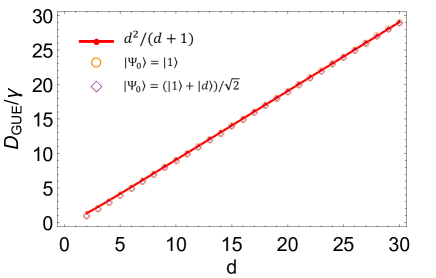
Figure SM1: Decoherence rates $D_{\mathrm{GUE}}/\gamma$ versus the dimension $d$ of chaotic decoherence channels sampled by random matrices. Analytical formula derived by Haar measure (red dots) is in comparison with numerical simulations over 20000 realizations of the GUE with fixed initial states $\left|\Psi_{0}\right\rangle=\left|1\right\rangle$ (orange circles), and $\left|\Psi_{0}\right\rangle=(\left|1\right\rangle+\left|d\right\rangle)/\sqrt{2}$ (purple diamonds), respectively.

Note that the above proof is completely strict with no approximation and valid for all dimensions. We can also employ the partition function method to the calculation of $D_{\mathrm{GUE}}$, which will include some approximations (see, e.g., in Section .4 for initial thermofield double states).

Equation (S10) provides an upper bound to the decoherence rate in GUE. The equality is achieved when the initial state is a pure fixed state, which is just the case we discuss in the main text. To verify Eq. (S10) as well as Eq. (4) in the main text, in Fig. (SM1), we choose the one decoherence channel as an example (i.e., $\mu=1$, and denote $\gamma_{\mu}=\gamma$) and compare the analytical expression with numerical simulations over 20000 realizations of the GUE for two different initial fixed pure states. In accordance with the proof, analytical results accurately match the decoherence rate obtained from the numerical simulations by averaging over different realizations of the Lindblad operators.

.1.3 3. Derivation of Eq. (S19)

1.— Proof of $\left\langle\text{tr}\left(\rho_{\beta=0}V_{\mu}^{2}\right)\right\rangle_{\mathrm{GUE}}=d/2$ in Eq. (S19).

Proof. In the following, we drop the subscript “$\mu$” temporarily for clarity

$$\left\langle\text{tr}\left(\rho_{\beta=0}V^{2}\right)\right\rangle_{\mathrm{GUE}}=\frac{1}{d}\left\langle\text{tr}\left(V^{2}\right)\right\rangle_{\text{{GUE}}}=\frac{1}{d}\left[\int v^{2}\varrho_{\mathrm{GUE}}(v)\mathrm{d}v\right].$$ (S20)

The eigenvalue density averaged over GUE is given by sBook-RMT

$$\varrho_{\mathrm{GUE}}(v)=\sum_{l=0}^{d-1}\phi_{l}(v)^{2},\text{ and }\phi_{l}(v):=\frac{e^{-\frac{v^{2}}{2}}\mathrm{H}_{l}(v)}{\sqrt{\sqrt{\pi}2^{l}l!}},$$ (S21)

where $\mathrm{H}_{l}(x)$ are the Hermite polynomials. Then we have

$$\int v^{2}\varrho_{\mathrm{GUE}}(v)\mathrm{d}v=\frac{1}{\sqrt{\pi}}\sum_{l=0}^{d-1}\frac{1}{2^{l}l!}\int e^{-v^{2}}\left[v\mathrm{H}_{l}(v)\right]^{2}\mathrm{d}v=\frac{1}{2}\sum_{l=0}^{d-1}(2l+1)=\frac{d^{2}}{2},$$ (S22)

where we have employed the equality $x\mathrm{H}_{k}(x)=\frac{1}{2}\mathrm{H}_{k+1}(x)+k\mathrm{H}_{k-1}(x)$ and the orthogonality of the Hermite polynomials. Substituting Eq. (S22) into Eq. (S20), we have $\left\langle\text{tr}\left(\rho_{\beta=0}V^{2}\right)\right\rangle_{\mathrm{GUE}}=d/2$. $\square$

2.— Proof of $\left\langle\text{tr}\left(\rho_{\beta=0}V_{\mu}\right)^{2}\right\rangle_{\mathrm{GUE}}=0$ in Eq. (S19).

Proof. As before, we drop the subscript “$\mu$” temporarily for clarity

$$\left\langle\text{tr}\left(\rho_{\beta=0}V\right)^{2}\right\rangle_{\mathrm{GUE}} = \frac{1}{d^{2}}\left\langle\text{tr}\left(V\right)^{2}\right\rangle_{\text{{GUE}}}$$ (S23)

$$= \frac{1}{d^{2}}\left[\int v^{2}\varrho_{\mathrm{GUE}}(v)\mathrm{d}v+\left[\int v\varrho_{\mathrm{GUE}}(v)\mathrm{d}v\right]^{2}+\int\int vv^{\prime}\varrho_{\mathrm{GUE}}^{c}(v,v^{\prime})\mathrm{d}v\mathrm{d}v^{\prime}\right],$$

where the first item is just Eq. (S22), and the rest items are from the 2-point correlation function $\varrho_{\mathrm{GUE}}(v,v^{\prime})=\varrho_{\mathrm{GUE}}(v)\varrho_{\mathrm{GUE}}(v^{\prime})+\varrho_{\mathrm{GUE}}^{c}(v,v^{\prime})$, with

$$\varrho_{\mathrm{GUE}}^{c}(v,v^{\prime}):=-\sum_{k,l=0}^{d-1}\phi_{k}(v)\phi_{l}(v)\phi_{k}(v^{\prime})\phi_{l}(v^{\prime})$$ (S24)

denoting the connected two-level correlation function sBook-RMT . As in the first proof, the second item in Eq. (S23) reads

$$\int v\varrho_{\mathrm{GUE}}(v)\mathrm{d}v=0.$$ (S25)

In the following, we focus on the third item in Eq. (S23)

$$\int\int vv^{\prime}\varrho_{\mathrm{GUE}}^{c}(v,v^{\prime})\mathrm{d}v\mathrm{d}v^{\prime} = -\sum_{k,l=0}^{d-1}\int v\phi_{k}(v)\phi_{l}(v)\mathrm{d}v\int v^{\prime}\phi_{k}(v^{\prime})\phi_{l}(v^{\prime})\mathrm{d}v^{\prime}$$ (S26)

$$= -\frac{1}{\pi}\sum_{k,l=0}^{d-1}\frac{1}{2^{k}k!2^{l}l!}\int ve^{-\frac{v^{2}}{2}}\mathrm{H}_{k}(v)\mathrm{H}_{l}(v)\mathrm{d}v\int v^{\prime}e^{-\frac{v^{\prime 2}}{2}}\mathrm{H}_{k}(v^{\prime})\mathrm{H}_{l}(v^{\prime})\mathrm{d}v^{\prime}$$

$$= -\frac{1}{2}\sum_{k=0}^{d-1}(2k+1)=-\frac{d^{2}}{2},$$

where we have employed the equality

$$\int xe^{-\frac{x^{2}}{2}}\mathrm{H}_{k}(x)\mathrm{H}_{l}(x)\mathrm{d}x=\frac{1}{2}\sqrt{\pi}(k+1)!2^{k+1}\delta_{l,k+1}+k\sqrt{\pi}(k-1)!2^{k-1}\delta_{l,k-1},$$ (S27)

which can be proved with the generating function $e^{2xt-t^{2}}=\sum_{k=0}^{\infty}\mathrm{H}_{k}(x)\frac{t^{k}}{k!}$ of Hermite polynomials. With Eq. (S25), Eq. (S26), and Eq. (S22), we have $\left\langle\text{tr}\left(\rho_{\beta=0}V\right)^{2}\right\rangle_{\mathrm{GUE}}\equiv 0$. $\square$

.2 B. Proof of inequality $\mathrm{var}_{{}_{\rho}}(X)\leq\left\|X\right\|^{2}$

Proof.

$$\begin{split}\mathrm{var}_{{}_{\rho}}(X)&=\text{tr}\left(\rho X^{2}\right)-\left[\text{tr}\left(\rho X\right)\right]^{2}\\ &\leq\text{tr}\left(\rho X^{2}\right)=\sum_{l}x_{l}^{2}\left\langle l\right|\rho\left|l\right\rangle\\ &\leq\max\{x_{l}^{2}\}\sum_{l}\left\langle l\right|\rho\left|l\right\rangle\\ &=x_{M}^{2}=\left\|X\right\|^{2},\end{split}$$ (S28)

where $x_{l}$ is the eigenvalue of $X$, $x_{M}$ is the maximum eigenvalue of $\sqrt{X^{{\dagger}}X}$, and $\left\|X\right\|$ is the spectral norm. $\square$

.3 C. Master equations for the dynamics of the noise-averaged density matrix

.3.1 1. Stochastic fluctuating master equations

The dynamics of the noise-averaged density matrix $\rho_{t}=\left\langle|\Psi_{t}^{\xi}\rangle\langle\Psi_{t}^{\xi}|\right\rangle_{\xi}$, with $\xi:=\{\xi_{t}^{\mu}\}$ for simplicity, can be derived using Novikov’s theorem sNovikov ; sChenu2017 . In this appendix we employ another method, i.e., Itô calculus, to derive the master equation. The stochastic Schrödinger equation of a quantum system $H_{0}$ perturbed by the real Gaussian white noises $\hbar\sum_{\mu}\sqrt{\gamma_{\mu}}\xi_{t}^{\mu}V_{\mu}$ is given by

$$i\hbar\frac{\mathrm{d}|\Psi_{t}^{\xi}\rangle}{\mathrm{d}t}=\left(H_{0}+\hbar\sum_{\mu}\sqrt{\gamma_{\mu}}\xi_{t}^{\mu}V_{\mu}\right)|\Psi_{t}^{\xi}\rangle,$$ (S29)

which, in the Itô form, can be written as

$$\mathrm{d}|\Psi_{t}^{\xi}\rangle=-\frac{i}{\hbar}H_{0}\mathrm{d}t|\Psi_{t}^{\xi}\rangle-i\sum_{\mu}\sqrt{\gamma_{\mu}}V_{\mu}\mathrm{d}W_{t}^{\mu}|\Psi_{t}^{\xi}\rangle-\frac{1}{2}\sum_{\mu}\gamma_{\mu}V_{\mu}^{2}\mathrm{d}t|\Psi_{t}^{\xi}\rangle,$$ (S30)

where $\mathrm{d}W_{t}^{\mu}$, defined from $\xi_{t}^{\mu}:=\mathrm{d}W_{t}^{\mu}/\mathrm{d}t$, is an Itô stochastic differential satisfying the standard Itô calculus rules, $\mathrm{d}W_{t}^{\mu}\mathrm{d}W_{t}^{\nu}=\delta_{\mu\nu}\mathrm{d}t$ and $\mathrm{d}W_{t}^{\mu}\mathrm{d}t=\mathrm{d}t^{2}=0$. According to the Leibnitz chain rule of Itô calculus, $\mathrm{d}(XY)=(\mathrm{d}X)Y+X\mathrm{d}Y+(\mathrm{d}X)(\mathrm{d}Y)$ sSSE-PRD , the corresponding Liouville-von Neumann equation for the density matrix $\rho_{t}^{\xi}=|\Psi_{t}^{\xi}\rangle\langle\Psi_{t}^{\xi}|$ is given by

$$\mathrm{d}\rho_{t}^{\xi}=-\frac{i}{\hbar}[H_{0},\rho_{t}^{\xi}]\mathrm{d}t-\frac{1}{2}\sum_{\mu}\gamma_{\mu}\left[V_{\mu},\left[V_{\mu},\rho_{t}^{\xi}\right]\right]\mathrm{d}t-i\sum_{\mu}\sqrt{\gamma_{\mu}}\left[V_{\mu},\rho_{t}^{\xi}\right]\mathrm{d}W_{t}^{\mu}.$$ (S31)

Taking the stochastic expectation of the above equation, and considering $\left\langle XdW_{t}^{\mu}\right\rangle_{\xi}=0$ sSSE-PRD gives the evolution equation for $\rho_{t}=\langle\rho_{t}^{\xi}\rangle_{\xi}$ as

$$\dot{\rho}_{t}=-\frac{i}{\hbar}[H_{0},\rho_{t}]-\frac{1}{2}\sum_{\mu}\gamma_{\mu}\left[V_{\mu},\left[V_{\mu},\rho_{t}\right]\right],$$ (S32)

which corresponds to a master equation with Hermitian Lindblad operators.

.3.2 2. Examples

Example 1.–Consider a general $k$-body long-range Ising model in a transverse-field $h$ with the following Hamiltonian

$$H_{0}=-\sum_{l_{1}<\cdots<l_{k}}^{n}J_{l_{1}<\cdots<l_{k}}\Lambda_{l_{1}<\cdots<l_{k}}-h\sum_{l}^{n}\sigma_{l}^{x},$$ (S33)

where $J_{l_{1}<\cdots<l_{k}}$ denote the coupling constants, $\Lambda_{l_{1}<\cdots<l_{k}}:=\sigma_{l_{1}}^{z}\otimes\cdots\otimes\sigma_{l_{k}}^{z}\otimes\mathds{1}_{\delta\neq l_{1},\cdots,l_{k}}$, and $\sigma^{\alpha}$ are the usual Pauli operators with $\alpha\in\{x,y,z\}$. By adding a single real Gaussian white noise to the coupling constants, i.e.,

$$J_{l_{1}<\cdots<l_{k}}\rightarrow J_{l_{1}<\cdots<l_{k}}+\hbar\sqrt{\gamma}\xi_{t},$$ (S34)

the noise-averaged density matrix obeys the master equation Eq. (S32), with a symmetric Lindblad operator

$$V=\sum_{l_{1}<\cdots<l_{k}}^{n}\Lambda_{l_{1}<\cdots<l_{k}}.$$ (S35)

Note that the same master equation arise from a variety of decoherence sources. In the present example, the decoherence source is the stochastic Gaussian white noise. In the main text, the Lindblad operator [i.e., Eq. (5) in the main text] of the $k$-body long-range interactions is general, independent of any specific decoherence sources.

Example 2.–Two-body random ensembles (TBRE) has received considerable attention in the theory of random matrices for many-body quantum systems. Here, we consider an embedded ensemble with random two-body interactions in a spin chain s2-bodyRE

$$H_{0}=\sum_{l=1}^{n-1}\sum_{\alpha,\alpha^{\prime}=x,y,z}A_{l,\alpha,\alpha^{\prime}}\sigma_{l}^{\alpha}\sigma_{l+1}^{\alpha^{\prime}}+\sum_{l=1}^{n}\sum_{\alpha=x,y,z}B_{l,\alpha}\sigma_{l}^{\alpha},$$ (S36)

where we have assumed the open boundary conditions, $A_{l,\alpha,\alpha^{\prime}}$ are the random two-body interaction variables, and $B_{l,\alpha}$ denote the random external fields. Similar to Example 1, a single real Gaussian white noise is added to the random two-body interaction variables

$$A_{l,\alpha,\alpha^{\prime}}\rightarrow A_{l,\alpha,\alpha^{\prime}}+\hbar\sqrt{\gamma}\xi_{t},$$ (S37)

the noise-averaged density matrix also obeys the master equation Eq. (S32), with a symmetric Lindblad operator

$$V=\sum_{l=1}^{n-1}\sum_{\alpha,\alpha^{\prime}=x,y,z}\sigma_{l}^{\alpha}\sigma_{l+1}^{\alpha^{\prime}}.$$ (S38)

Then the decoherence rate will be bounded by $D\leq 2\gamma\left\|V\right\|^{2}\leq 162\gamma(n-1)^{2},$ where we have used $\left\|\sigma_{l}^{\alpha}\sigma_{l+1}^{\alpha^{\prime}}\right\|=1$. Obviously, the decoherence rate of this two-body random ensembles model will increase at most in a polynomial way.

Example 3.–We consider a composite system describing two non-interacting subsystems Hamiltonian

$$\tilde{H}_{0}=H\otimes\mathds{1}+\mathds{1}\otimes H,$$ (S39)

that are independently perturbed by Gaussian real white noises $H\rightarrow(1+\hbar\sqrt{\gamma}\xi_{t}^{L(R)})H$. As a result, the dynamic is generated by the fluctuating (stochastic) Hamiltonian

$$\tilde{H}_{t}=H\otimes\mathds{1}+\mathds{1}\otimes H+\hbar\sqrt{\gamma}(\xi_{t}^{L}H\otimes\mathds{1}+\mathds{1}\otimes\xi_{t}^{R}H).$$ (S40)

Assuming $\xi_{t}^{L}\neq\xi_{t}^{R}$, the noise-averaged density matrix obeys the master equation Eq. (S32), with $\mu\in\{1,2\}$ and the following choice of the Lindblad operators

$$\tilde{V}_{1}=H\otimes\mathds{1},\text{ and }\tilde{V}_{2}=\mathds{1}\otimes H.$$ (S41)

Note that the above example concerns the setting in which we discussed the decoherence of a thermofield double state case in the main text.

We also note that decoherence in the energy eigenbasis arises as well from uncertainties in the measurement of time sE1 ; sE2 , due to the inability to physically determine the value of the ideal time parameter $t$ with arbitrary precision. If one is limited to a non-ideal clock, the observed evolution in terms of a physical time parameter is effectively non-unitary, satisfying Eq. (S32) with Lindblad operators $\widetilde{V}=H\otimes\mathds{1}+\mathds{1}\otimes H$, where the constant $\gamma$ depends on the clock precision. Here, two alternatives open up: either time intervals can be determined with arbitrary precision, or the laws of physics put fundamental constraints on it. The latter case has been proposed by a combination of general relativity and quantum mechanics arguments sE1 ; sE2 , in which the loss of unitary is considered fundamental.

.4 D. Decoherence rate of the thermofield double (TFD) state in GUE

.4.1 1. Decoherence dynamics of the TFD state

The analysis in the main text is focused on the decoherence time extracted from the short-time asymptotics of the purity decay. Under dephasing, the purity decay is monotonic as a function of time. Thus, the decoherence rates provide a conservative estimate to the actual decay dynamics and the rate is expected to decrease as a function of time. To analyze the complete dynamics we consider the master equation governing the density matrix of the composite system with stochastic Hamiltonian. For a single realization of the noise, the dynamics is described by the Liouville-von Neumann equation

$$\dot{\rho}_{t}^{\mathrm{\xi}}=\frac{-i}{\hbar}[(H\otimes\mathds{1}+\mathds{1}\otimes H)+\hbar\sqrt{\gamma}(\xi_{t}^{L}H\otimes\mathds{1}+\mathds{1}\otimes\xi_{t}^{R}H),\rho_{t}^{\mathrm{\xi}}].$$ (S42)

The dynamics of the average density matrix over many realizations of the noise reads, from (S32), [also see Example 2 in Section C]

$$\dot{\rho}_{t}=\frac{-i}{\hbar}[(H\otimes\mathds{1}+\mathds{1}\otimes H),\rho_{t}]-\frac{\gamma}{2}[H\otimes\mathds{1},[H\otimes\mathds{1},\rho_{t}]]-\frac{\gamma}{2}[\mathds{1}\otimes H,[\mathds{1}\otimes H,\rho_{t}]],$$ (S43)

with the initial state being given by

$$\rho_{0} = |\Phi_{0}\rangle\langle\Phi_{0}|$$ (S44)

$$= \frac{1}{Z(\beta)}\sum_{k,\ell}e^{-\frac{\beta}{2}(E_{k}+E_{\ell})}|k\rangle|k\rangle\langle\ell|\langle\ell|,$$

for a given operator $H$, where $E_{k(\ell)}$ are the corresponding eigenvalues.

The operators in Eq. (S43) being in their diagonal basis, the time-evolution of the density matrix can be obtained in a closed form as

$$\dot{\rho}_{kk,\ell\ell}=\frac{2}{i\hbar}(E_{k}-E_{\ell}){\rho}_{kk,\ell\ell}-\gamma(E_{k}-E_{\ell})^{2}{\rho}_{kk,\ell\ell}.$$ (S45)

Thus, the exact time-dependent density matrix is given by

$$\rho_{t} = \sum_{k,\ell}{\rho}_{kk,\ell\ell}(t=0)e^{-i\frac{2t}{\hbar}(E_{k}-E_{\ell})-\gamma t(E_{k}-E_{\ell})^{2}}|k\rangle|k\rangle\langle\ell|\langle\ell|$$ (S46)

$$= \frac{1}{Z(\beta)}\sum_{k,\ell}e^{-\frac{\beta}{2}(E_{k}+E_{\ell})}e^{-i\frac{2t}{\hbar}(E_{k}-E_{\ell})-\gamma t(E_{k}-E_{\ell})^{2}}|k\rangle|k\rangle\langle\ell|\langle\ell|.$$

We note that the fixed-point of the evolution

$$\rho_{\infty}=\frac{1}{Z(\beta)}\sum_{k}e^{-\beta E_{k}}|k\rangle|k\rangle\langle k|\langle k|,$$ (S47)

is a separable state. Thus, as $t\rightarrow\infty$ the off-diagonal elements (so-called coherences) of the density matrix decay to zero, showing that entanglement is lost in the decoherence process.

The purity of the time-dependent density matrix decays, as the time of evolution goes by, according to

$$P_{t}=\frac{1}{Z(\beta)^{2}}\sum_{k,\ell}e^{-\beta(E_{k}+E_{\ell})-2\gamma t(E_{k}-E_{\ell})^{2}}.$$ (S48)

At long-times, it saturates at the value

$$P_{\infty}=\frac{1}{Z(\beta)^{2}}\sum_{k}e^{-2\beta E_{k}}=\frac{Z(2\beta)}{Z(\beta)^{2}},$$ (S49)

which is precisely the purity of a canonical thermal state. This long-time asymptotic limit is shared by the unitary dynamics sDyer17 ; sdelCampo17prd .

For arbitrary $t$, we make use of the Hubbard-Stratonovich transformation to write

$$e^{-2t\gamma(E_{k}-E_{\ell})^{2}}=\sqrt{\frac{1}{8\pi\gamma t}}\int_{-\infty}^{\infty}e^{-\frac{y^{2}}{8\gamma t}}e^{-iy(E_{k}-E_{\ell})}\mathrm{d}y.$$ (S50)

This yields the following expression for the purity

$$P_{t}=\sqrt{\frac{1}{8\pi\gamma t}}\int_{-\infty}^{\infty}e^{-\frac{y^{2}}{8\gamma t}}\left|\frac{Z(\beta-iy)}{Z(\beta)}\right|^{2}\mathrm{d}y,$$ (S51)

in terms of the analytic continuation of the partition function. The later has been extensively studied as a characterization of the spectral properties of quantum chaotic systems as well as a proxy for information scrambling; see sDyer17 ; sdelCampo17prd and references therein.

We are interested in the ensemble dynamics of the purity $P_{t}$ with $H\in$ GUE, i.e.,

$$\left\langle P_{t}\right\rangle_{\text{{GUE}}}=\sqrt{\frac{1}{8\pi\gamma t}}\int_{-\infty}^{\infty}e^{-\frac{y^{2}}{8\gamma t}}\left\langle\left|\frac{Z(\beta-iy)}{Z(\beta)}\right|^{2}\right\rangle_{\text{{GUE}}}\mathrm{d}y.$$ (S52)

We rely on the annealing approximation to simplify its computation

$$\left\langle P_{t}\right\rangle_{\text{{GUE}}}\dot{=}\frac{1}{\left\langle Z(\beta)^{2}\right\rangle_{\text{{GUE}}}}\sqrt{\frac{1}{8\pi\gamma t}}\int_{-\infty}^{\infty}e^{-\frac{y^{2}}{8\gamma t}}\left\langle\left|Z(\beta-iy)\right|^{2}\right\rangle_{\text{{GUE}}}\mathrm{d}y,$$ (S53)

the accuracy of which is well-established (see, e.g. Ref. sChenu18 ). Explicit expressions for both $\left\langle Z(\beta)^{2}\right\rangle_{\text{GUE}}$ and $\left\langle\left|Z(\beta-iy)\right|^{2}\right\rangle_{\text{{GUE}}}$ for finite dimensional Hilbert space dimension can be calculated with the polynomial method introduced in Sec. .1.3 (also see, e.g. Ref. sChenu18 ).

.4.2 2. Derivation of decoherence rate of the TFD state — Eq. (13)

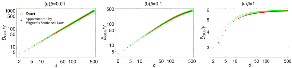
Figure SM2: Decoherence rates $\tilde{D}_{\mathrm{GUE}}/\gamma$ versus dimension $d$ with exact random matrices theory [Eq. (S56)] (green circles) and Wigner’s semicircle approximations [Eq. (S59)] (red dots), displayed for (a) $\beta=0.01$; (b) $\beta=0.1$; and (c) $\beta=1$, respectively.

The partition function of thermofield double states under the average over GUE is given by

$$\left\langle Z(\beta)\right\rangle_{\text{{GUE}}}=\int\varrho_{\text{{GUE}}}(E)e^{-\beta E}\mathrm{d}v,$$ (S54)

with the averaged spectral density $\varrho_{\text{{GUE}}}(E)$ mentioned in Eq. (S21) ($v\rightarrow$ $E$). By using the integration of Hermite polynomials $\int\mathrm{d}xe^{-(x+a)^{2}}\mathrm{H}_{n}(x)\mathrm{H}_{m}(x)=\sqrt{\pi}2^{n}n!(-2a)^{m-n}\mathrm{L}_{n}^{(m-n)}(-2a^{2})$ for $n\leq m$ sBook-Int , we have

$$\begin{split}\left\langle Z(\beta)\right\rangle_{\text{{GUE}}}&=\sum_{l=0}^{d-1}\frac{1}{2^{l}l!\sqrt{\pi}}e^{\frac{\beta^{2}}{4}}\int e^{-(E+\frac{\beta}{2})^{2}}\mathrm{H}_{l}(E)^{2}\mathrm{d}E\,\\ &=e^{\frac{\beta^{2}}{4}}\sum_{l=0}^{d-1}\mathrm{L}_{l}\left(-\frac{\beta^{2}}{2}\right)\\ &=e^{\frac{\beta^{2}}{4}}\mathrm{L}_{d-1}^{(1)}\left(-\frac{\beta^{2}}{2}\right),\end{split}$$ (S55)

where $\mathrm{L}_{n}(x)$ are the Laguerre polynomials and $\mathrm{L}_{n}^{(\alpha)}(x)$ are the generalized Laguerre polynomials satisfying the recurrence relation $\mathrm{L}_{n}^{(\alpha+1)}(x)=\sum_{l=0}^{n}\mathrm{L}_{l}^{(\alpha)}(x)$, with $\mathrm{L}_{n}^{(0)}(x)=\mathrm{L}_{n}(x)$. Then the decoherence rate is given, from Eq. (11) in the main text and using the annealing approximation (see, e.g., Sec. .4.3), by

$$\tilde{D}_{\text{{GUE}}} \dot{=} 4\gamma\frac{\mathrm{d}^{2}}{\mathrm{d}\beta^{2}}\ln\left\langle Z(\beta)\right\rangle_{\text{{GUE}}}$$ (S56)

$$= 2\gamma\Big{[}1+2\mathrm{F}_{1}^{(2)}\left({-}\beta^{2}/2\right)-2\beta^{2}\left(\mathrm{F}_{1}^{(2)}\big{(}{-}\beta^{2}/2\big{)}\right)^{2}+2\beta^{2}\mathrm{F}_{1}^{(3)}\left({-}\beta^{2}/2\right)\Big{]},\text{ }$$

with F${}_{l}^{(m)}(x):=\mathrm{L}_{d-m}^{(m)}(x)/\mathrm{L}_{d-l}^{(l)}(x)$.

In the large dimension case, the eigenvalue density of $E$ over Gaussian random matrices average obeys the Wigner’s semicircle law

$$\varrho_{\text{{GUE}}}(E)=\frac{\sqrt{2d}}{\pi}\sqrt{1-\left(\frac{E}{\sqrt{2d}}\right)^{2}},$$ (S57)

with $E\in[-\sqrt{2d},\sqrt{2d}]$ sBook-RMT . Then, the partition function Eq. (S55) is given by sdelCampo17prd

$$\left\langle Z(\beta)\right\rangle_{\text{{GUE}}}=\frac{\sqrt{2d}\mathrm{I}_{1}(\sqrt{2d}\beta)}{\beta},$$ (S58)

where $\mathrm{I}_{n}(x)$ is the modified Bessel function of first kind and order $n$. Using the fact that $I_{0}(x)=I_{2}(x)+(2/x)I_{1}(x)$, this leads to

$$\tilde{D}_{\mathrm{GUE}}=8\gamma d\left[1-\frac{3}{\sqrt{2d}\beta}g(\sqrt{2d}\beta)-g(\sqrt{2d}\beta)^{2}\right],$$ (S59)

with $g(x):=\mathrm{I}_{2}(x)/\mathrm{I}_{1}(x)$. Equation (S59) corresponds to Eq. (11) in the main text.

According to Wigner’s semicircle law, when the dimension is large, Eq. (S59) matches Eq. (S56) perfectly. In addition, numerical simulations show that when $\beta\ll 1$, Eq. (S59) also well agrees with Eq. (S56), even when the dimension is not large [shown in Fig. SM2].

.4.3 3. Annealing approximation

In this section, we provide a brief instruction for the annealing approximation used in Eq. (S56). To simplify the calculations, we make use of the annealed average over logarithm of the partition function $\ln Z(\beta)$, i.e.,

$$\left\langle\ln[Z(\beta)]\right\rangle_{\text{{GUE}}}\doteq\ln\left\langle Z(\beta)\right\rangle_{\text{{GUE}}}.$$ (S60)

In fact, according to Jensen’s inequality $\left\langle\ln[Z(\beta)]\right\rangle_{\text{{GUE}}}\leq\ln\left\langle Z(\beta)\right\rangle_{\text{{GUE}}}$, since $\ln(x)$ is a concave function. The equality is well satisfied in high dimensional systems (when the dimension is not large, the annealing approximation is still valid in high temperature regime), as verified by numerical simulations; see Fig. SM3.

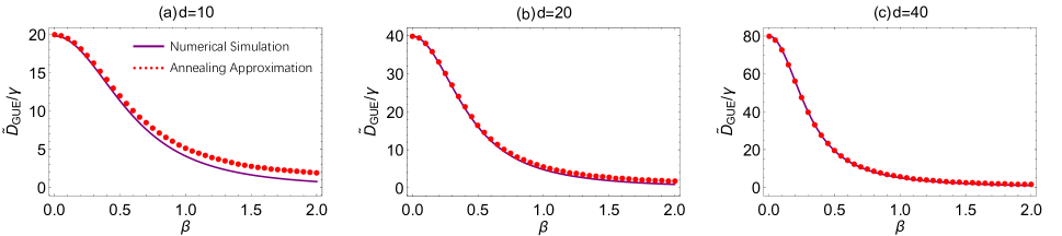
Figure SM3: Decoherence rates $\tilde{D}_{\mathrm{GUE}}/\gamma$ versus $\beta$ of thermofield double states in GUE with exact numerical simulations (solid line) and annealing approximations (red dots) respectively. The numerical average is performed over 2000 realizations of the GUE with the dimension (a) $d=10$; (b) $d=20$; and (c) $d=40$, respectively.

References

(1) M. L. Mehta, Random Matrices, 3rd
Edition (Elsevier, San Diego, 2004).
(2) F. Mezzadri and N. C. Snaith, Recent
Perspectives in Random Matrix Theory and Number Theory (Cambridge
University Press, New York, 2010) p.36.
(3) T. Tao, Topics in Random Matrix Theory (American Mathematical Society, Rhode Island, 2012) p.184.
(4) J. Diestel and A. Spalsbury, The Joys of Haar Measure (American Mathematical Society, Providence, 2014) p.161.