Prospects of detecting a large-scale anisotropy of ultra-high-energy cosmic rays from a nearby source with the K-EUSO orbital telescope

Abstract

KLYPVE-EUSO (K-EUSO) is a planned orbital detector of ultra-high-energy cosmic rays (UHECRs), which is to be deployed on board the International Space Station. K-EUSO is expected to have a uniform exposure over the celestial sphere and register from 120 to 500 UHECRs at energies above 57 EeV in a 2-year mission. We employed the TransportCR and CRPropa 3 packages to estimate prospects of detecting a large-scale anisotropy of ultra-high-energy cosmic rays from a nearby source with K-EUSO. Nearby active galactic nuclei Centaurus A, M82, NGC 253, M87 and Fornax A were considered as possible sources of UHECRs. A minimal model for extragalactic cosmic rays and neutrinos by Kachelrieß, Kalashev, Ostapchenko and Semikoz (2017) was chosen for definiteness. We demonstrate that an observation of $\gtrsim 300$ events will allow detecting a large-scale anisotropy with a high confidence level providing the fraction of from-source events is $\simeq$10–15%, depending on a particular source. The threshold fraction decreases with an increasing sample size. We also discuss if an overdensity originating from a nearby source can be observed at around the ankle in case a similar anisotropy is found beyond 57 EeV. The results are generic and hold for other future experiments with a uniform exposure of the celestial sphere.

Introduction

Ultra-high-energy cosmic rays (UHECRs) with energies above $\sim 50$ EeV, sometimes called extreme-energy cosmic rays, were first registered almost 60 years ago [1] but their nature and sources still remain an open problem of astrophysics and cosmic ray physics. UHECRs are supposed to be produced in extragalactic sources and this has been recently corroborated by an observational finding of the dipole anisotropy in the arrival directions of UHECRs with energies above 8 EeV [2]. Different classes of astrophysical objects are considered as possible sources of UHECRs, among them gamma-ray bursts [3, 4, 5], young millisecond pulsars and magnetars [6, 7, 8], tidal disruption events [9, 10, 11], active galactic nuclei (AGN) of different types [12] and mechanisms of acceleration, including blazars [13, 14], black hole jets [15, 16, 17] and several other, see, e.g., [18] for a more in-depth discussion.

In this work, we focus on possible large-scale anisotropy signatures of a model by Kachelrieß, Kalashev, Ostapchenko and Semikoz [19] (KKOS in what follows). We use the model as a benchmark scenario which represents a much broader class of models with strong nearby UHECR sources and an intermediate composition, rather than something unique. Although some particular features of other models can vary, we expect our estimations might be true for them as well.

The KKOS model can explain the observed energy spectrum and mass composition of cosmic rays (CR) with energies above $\sim 10^{17}$ eV, and matches the high-energy neutrino flux measured by IceCube. The scenario assumes that UHECRs are produced by (possibly a subclass of) AGN. The model does not rely on any particular acceleration mechanism, although it was shown that UHECR production could proceed either via shock acceleration in accretion shocks [20] or via acceleration in regular fields [21, 22, 23, 24, 25] close to a supermassive black hole (SMBH). Alternatively, UHECRs could be produced in large-scale radio jets [26] or via a two-step acceleration process in the jet and a radio-lobe [27]. The model neglects the acceleration process details and just relies on the following basic assumptions: (i) the energy spectra of nuclei after the acceleration phase follow a power-law with a rigidity dependent cutoff

$$j_{\mathrm{inj}}(E)\propto E^{-\alpha}\exp[-E/(ZE_{\max})]\,;$$

(ii) the CR nuclei diffuse first through a zone dominated by photo-hadronic interactions, and then they escape into a second zone dominated by hadronic interactions with gas. It was shown that a good fit to the CR energy spectrum can be obtained assuming only hadronic interactions of UHECRs with gas around their sources, but it was difficult to reproduce the observed distribution of $X_{\max}$ of CR-induced air showers. Only after adding photo-nuclear interactions with a relatively large interaction depth, which suggests that UHECRs are accelerated close to SMBHs, it was possible to reduce significantly the fraction of heavy nuclei in the primary fluxes and therefore fit satisfactorily both the spectrum and composition data on UHECRs. Moreover, the secondary high-energy neutrino flux obtained in the scenario matches the IceCube measurements [28], while the contribution of unresolved UHECR sources to the extragalactic $\gamma$-ray background [29] is of the order of 30%.

The spectrum of CR leaving the source environment (i.e., after passing the second zone) in the best fit obtained with the KKOS model for $\alpha=1.5$ is shown in the left panel of Fig. 1 for several mass ranges. In the right panel, we illustrate the attenuation effect on the integral flux by plotting the distance at which the total flux above the given energy drops by factor of $1/e$. Note that the integral flux attenuation length depends both on the initial source spectrum and composition.

Due to strong propagation effects, the observable cosmic ray mass composition and energy spectrum can vary considerably for each individual source even though the injection spectrum is precisely the same for all of them. Moreover, at energies $E\simeq 150$ EeV, where the attenuation length for the integral flux drops to tens of Mpc, the CR flux may be dominated by the contribution of a nearby source located within 20 Mpc from the Milky Way. This, in turn, can lead to a substantial large-scale anisotropy in the UHECR flux. Orbital detectors with a sufficiently large exposure will provide good opportunities for studying this effect due to their possibly almost uniform exposure of the whole celestial sphere [30, 31, 32].

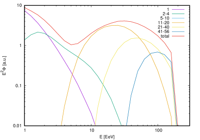
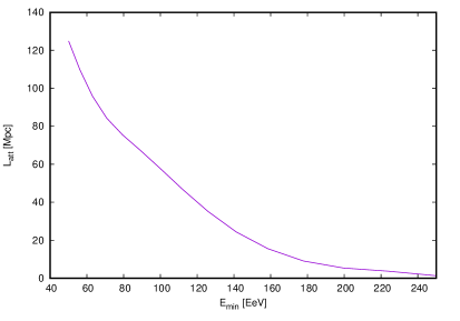
Figure 1: The effective CR source energy spectrum for different mass components (left) and integral flux above $E_{\text{min}}$ suppression length (right) in the KKOS model.

One of the future orbital experiments that are being actively developed today is the KLYPVE-EUSO (K-EUSO) telescope, which is aimed to be installed on board the International Space Station (ISS) in 2022 for a 2-year mission [33, 34, 35, 36]. K-EUSO is a further development of a technique of registering UHECRs via ultra-violet radiation emitted by extensive air showers in the atmosphere of Earth from a low-orbit satellite, implemented for the first time in the TUS detector [37, 38]. The telescope is expected to have a Schmidt-type optical system with the main mirror-reflector of a 4 m diameter, an entrance pupil of a 2.5 m diameter and a 1.7 m focal length. A round-shaped field of view of $40^{\circ}$ will provide an instantaneous geometrical area of nearly $6.7\times 10^{4}$ km² at sea level for the ISS altitude around 400 km. It is expected that K-EUSO will register from 120 up to almost 500 UHECRs with energies above 57 EeV in two years. The difference between the lower and the upper boundaries of the estimate arises from the difference in the energy spectra of the Pierre Auger Observatory and the Telescope Array [36]. Capabilities of the previous version of K-EUSO (KLYPVE) to detect the Telescope Array hotspot were studied earlier [39].

In what follows, we study if K-EUSO will be able to detect a large-scale anisotropy of arrival directions of UHECRs with energies above 57 EeV originating in a nearby AGN in the KKOS model. However, the presented results are valid for any other future experiment with a uniform exposure of the celestial sphere, including the POEMMA mission [40].

1 Method of the analysis

In what follows, we consider five possible sources of UHECRs that are often discussed in literature and satisfy the KKOS model, namely, NGC 253, Centaurus A, M82, M87 and Fornax A. These are radio-loud galaxies located at distances $d\approx 3.5\dots 20$ Mpc from the Milky Way. For each source located at a given distance $d$, we calculated the energy spectrum and mass composition of the CR flux crossing the Milky Way boundary using a public numerical code TransportCR [43], which was also used in the original work [19]. A contribution of other sources was approximated by an isotropic component. The spectrum and mass composition for the isotropic component was calculated by solving the transport equation with a homogeneous source distribution for distances $R>2^{1/3}d$, and zero density for smaller distances.

We assumed that deflections of CR nuclei in the inter-galactic space are small, so that nuclei accelerated at a particular source arrive to the Milky Way within $1^{\circ}$ from the actual direction to the source. The CRPropa 3 package [44] (GitHub snapshot of 24th June, 2018) with the Jansson–Farrar model of the Galactic magnetic field (GMF) [45] was employed to calculate deflections of nuclei in the Galaxy on their way to the Solar system. All three components of the GMF present in the model (the regular, striated and turbulent ones) were utilised in simulations. Backtracking was performed for all possible pairs $(Z,E)$ in the spectra to obtain maps of apparent arrival directions of different nuclei to Earth given original directions of approaching the Milky Way. Calculations were made on the HEALPix grid with $N_{\mathrm{side}}=512$ providing an angular resolution of the order of $7^{\prime}$. This is far beyond the angular resolution of the K-EUSO experiment. It was chosen to reliably recover an observed distribution of arrival directions of nuclei after their propagation in the Galactic magnetic field.

There are a number of mathematical tools traditionally used for studying the large-scale anisotropy of cosmic rays. Historically the first one is the harmonic analysis in right ascension, see [2] for a recent application. In practice, the effectiveness of the method is mostly confined to the lowest multipoles due to the small statistics of UHECRs. Another approach is based on calculating the angular power spectrum, see, e.g., [46, 47]. We performed the respective analysis by preparing maps of the relative intensity of the CR flux

$$\delta I_{i}=\frac{N_{i}-\langle N\rangle_{i}}{\langle N\rangle_{i}},$$ (1.1)

where $N_{i}$ and $\langle N\rangle_{i}$ are the number of “observed” events and the number of “reference” events assuming the isotropic flux in the $i$th pixel of the HEALPix map. Coefficients of the angular power spectrum

$$C_{\ell}=\frac{1}{2\ell+1}\sum_{m=-\ell}^{+\ell}|a_{\ell m}|^{2}$$ (1.2)

were calculated using the anafast program of HEALPix. Coefficients $a_{\ell m}$ in Eq. (1.2) are the multipolar moments of the spherical harmonics used to decompose the relative intensity $\delta I_{i}$, defined in Eq. (1.1). Notice the coefficient $C_{0}=0$ in our case since $\delta I_{i}$ does not include the angular average.

The IceCube and Auger experiments suggested a simple approach that allows estimating the total impact of different multipoles in deviating from an isotropic distribution of arrival directions and also penalises statistically the search over many angular scales [48, 49]. They suggested to calculate an estimator

$$D^{2}(\text{sample})=\frac{1}{\ell_{\mathrm{max}}}\sum_{\ell=1}^{\ell_{\mathrm{max}}}\left(\frac{C_{\ell,\mathrm{sample}}-\langle C_{\ell,\mathrm{iso}}\rangle}{\sigma_{\ell,\mathrm{iso}}}\right)^{2},$$ (1.3)

where “sample” is either “data” when applied to experimental data or “iso” when applied to estimate the deviation of one isotropic sample from an averaged isotropic flux. Variables $C_{\ell,\mathrm{sample}}$, $\langle C_{\ell,\mathrm{iso}}\rangle$ and $\sigma_{\ell,\mathrm{iso}}$ are, respectively, the $C_{\ell}$ observed in the sample (either “data” or “iso”), and the average and the standard deviation of $C_{\ell}$ for isotropic expectations, all of them calculated at a given scale $\ell$. In practice, $\langle C_{\ell,\mathrm{iso}}\rangle$ and $\sigma_{\ell,\mathrm{iso}}$ are evaluated using a simulated isotropic flux with the same number of events and exposure as for the data [49]. One can choose a certain confidence level for defining a threshold to accept or reject the isotropy hypothesis and then compare a value of $D^{2}(\mathrm{data})$ calculated for the data to the distribution of $D^{2}(\mathrm{iso})$ obtained for the isotropic flux.

We tried this approach but found another function to be slightly more sensitive to deviations from an isotropic distribution than the one given by Eq. (1.3). Namely, all results presented below are based on calculating an estimator

$$D(\text{sample})=\frac{1}{\ell_{\mathrm{max}}}\sum_{\ell=1}^{\ell_{\mathrm{max}}}\frac{C_{\ell,\mathrm{sample}}-\langle C_{\ell,\mathrm{iso}}\rangle}{\sigma_{\ell,\mathrm{iso}}},$$ (1.4)

which is the same as the one used by the Pierre Auger Collaboration but without the square of the summands. This allows taking into account the fact that the expected deviations from the isotropic case are one-sided (positive). Since we are using simulated data instead of experimental results, the $C_{\ell,\mathrm{data}}$ coefficients in Eq. (1.3) are to be replaced with $C_{\ell,\mathrm{mix}}$, which denote $C_{\ell}$ obtained for a simulated mixture of an isotropic flux and cosmic rays arriving from a particular source. Contrary to the case when one employs experimental data, we needed to simulate many mixed samples to obtain the distribution of $D(\mathrm{mix})$ for each source.

2 Main results

Let us consider the simplest case of a large-scale anisotropy arising from an impact of a single source. Both $D(\mathrm{iso})$ and $D(\mathrm{mix})$ are random variables in our case, thus one needs to compare their distributions. As the null hypothesis, we assume that arrival directions of a mixed sample of UHECRs obey an isotropic distribution. We adopted the value of the error of the second kind $\beta=0.05$ and searched for a fraction $F_{1}/F_{\mathrm{tot}}$ of from-source events in the total flux such that the error of the first kind $\alpha\lesssim 0.01$. We performed simulations for $N_{\mathrm{UHECR}}=100,200,\dots,500$ to cover the whole possible range of UHECRs to be detected by K-EUSO above 57 EeV. The main results are presented in Tables 1 and 2.

The numbers in Table 1 give the percentage of events arriving from a particular source in a sample of size $N_{\mathrm{UHECR}}$, such that the above condition is satisfied ($\beta=0.05$, $\alpha\lesssim 0.01$). Table 2 provides actual values of $\alpha$ found in each case. For example, the error of the first kind $\alpha\approx 0.004$ as soon as the fraction of events arriving from Cen A in the otherwise isotropic sample of the size $N_{\mathrm{UHECR}}=500$ is $\geq 9\%$. Thus, Table 1 provides the percentage of from-source events in the whole sample that will allow detecting a large-scale anisotropy of UHECRs arriving from a particular source with a sufficiently small error of the first kind.

Table 1: Percentage of UHECRs arriving from five candidate sources in samples of sizes $N_{\mathrm{UHECR}}=100,\dots,500$ such that the error of the first kind $\alpha\lesssim 0.01$ for the null hypothesis of isotropy providing the second kind error $\beta=0.05$. The accuracy of the numbers is $\pm 1$.

$N_{\mathrm{UHECR}}$	100	200	300	400	500
NGC 253	17	12	10	8	7
Cen A	21	14	12	10	9
M82	26	18	14	12	11
M87	29	20	16	14	12
Fornax A	19	13	11	9	8

Table 2: Probabilities of the first kind errors $\alpha$ for the percentage of from-source events given in Table 1.

$N_{\mathrm{UHECR}}$	100	200	300	400	500
NGC 253	0.007	0.004	0.002	0.008	0.010
Cen A	0.006	0.010	0.003	0.005	0.004
M82	0.009	0.006	0.009	0.008	0.003
M87	0.006	0.005	0.005	0.003	0.007
Fornax A	0.007	0.009	0.003	0.009	0.009

All results presented in Tables 1 and 2 were obtained for 500,000 isotropic samples and at least 10,000 mixed samples for each $N_{\mathrm{UHECR}}$. Results for $N_{\mathrm{UHECR}}=500$ are illustrated in Figures 2–6 for each of the sources. It is interesting to mention that a fraction of $D(\mathrm{iso})$ greater than the median value of $D(\mathrm{mix})$ is $\lesssim 10^{-5}$ in all cases shown. Thus, the isotropy hypothesis will be rejected with a high confidence level for a typical sample.

An important point to mention is the value of $\ell_{\mathrm{max}}$ used for calculating the estimator $D$ defined in Eq. (1.4). It became clear from simulations and can be seen in Figures 2–6 that the coefficients $C_{\ell}$ calculated for mixed samples quickly converge to isotropic values, so that it usually makes little sense to take into account a contribution from multipoles with $\ell>16$. All results in terms of $D$ presented here were obtained with one and the same $\ell_{\mathrm{max}}=16$ for the sake of uniformity even it is not necessarily optimal, see below.

Let us briefly comment on the numbers obtained for each of the sources and presented in Tables 1 and 2.

The first three sources (NGC 253, Cen A and M82) are the closest among them. They are located at distances $d\approx 3.5$ Mpc [50] at different positions in the celestial sphere. Arrival directions of nuclei coming from them demonstrate strikingly different patterns, see the top panels in Figs. 2–4. The behaviour of $C_{\ell}$ is specific for each of the sources (see the left bottom panels), and the more fuzzy is the pattern of arrival directions of from-source UHECRs, the greater is their fraction in the whole sample necessary to distinguish a large-scale anisotropy. The percentage of from-source events required to reject the null hypothesis with $\alpha\lesssim 0.01$ varies in the range from 7% to 11% for $N_{\mathrm{UHECR}}=500$, and it grows with decreasing $N_{\mathrm{UHECR}}$ approximately inverse-proportionally to $\sqrt{N_{\mathrm{UHECR}}}$. The latter is true for all the other sources.

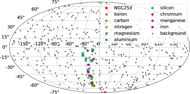
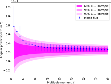
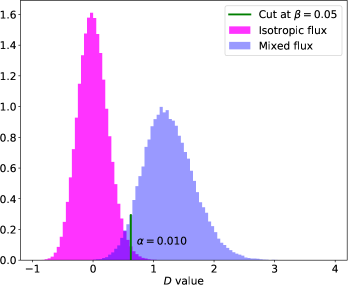
Figure 2: The case of $N_{\mathrm{UHECR}}=500$ and 7% events coming from NGC 253. Top panel: an example of a possible pattern of arrival directions. UHECRs that form an isotropic background are shown with small open circles. UHECRs arriving from the source are shown with coloured circles according to the type of the respective nucleus. The position of the source is indicated by the star. The map is shown in Galactic coordinates in the Mollweide projection. Left bottom panel: angular power spectrum $C_{\ell}$ for isotropic and mixed samples. Confidence intervals for 68%, 95% and 99% levels are shown with different shades of magenta for the isotropic distribution. Blue dots with error bars indicate $C_{\ell}$ for 50,000 mixed samples of size 500 with 7% events in each sample coming from the source. Right bottom panel: the histograms show empirical probability distribution functions of $D(\mathrm{iso})$ and $D(\mathrm{mix})$ calculated according to Eq. (1.4). The vertical red line marks a value of $D(\mathrm{mix})$ such that only 5% of all $D(\mathrm{mix})$ values are less than this particular value. This corresponds to the error of the second kind $\beta=0.05$. The error of the first kind $\alpha$ is also indicated in the panel.

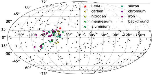
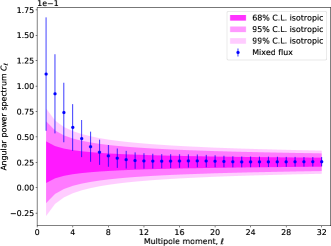
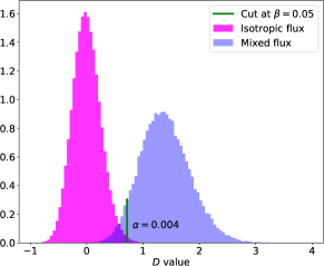
Figure 3: The case of $N_{\mathrm{UHECR}}=500$ and 9% events coming from Cen A. See the caption of Fig. 2 for other details.

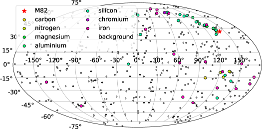
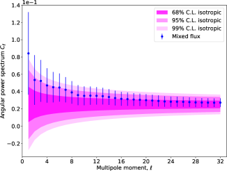
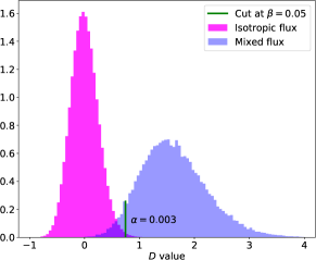
Figure 4: The case of $N_{\mathrm{UHECR}}=500$ and 11% events coming from M82. See the caption of Fig. 2 for other details.

Next, M87 (Virgo A) is an active galactic nucleus located in the Northern hemisphere at $d\approx 18.5$ Mpc from the Milky Way [50]. It provides a specific pattern of arrival directions of from-source UHECRs, distinct from the other sources considered here, see Fig. 5. The pattern is comparatively fuzzy, resulting in a slightly higher fraction of from-source events necessary to find an anisotropy.

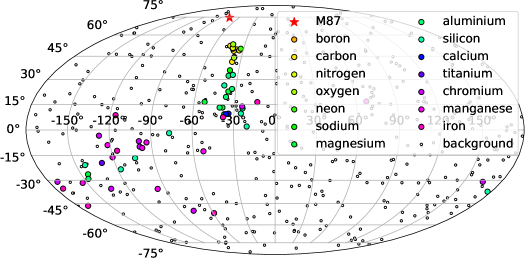
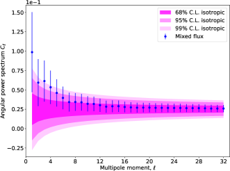
Figure 5: The case of $N_{\mathrm{UHECR}}=500$ and 12% events coming from M87. See the caption of Fig. 2 for other details.

Finally, the radio-loud Fornax A (NGC 1316) galaxy is the most distant source among those considered here, with $d\approx 20$ Mpc. A pattern of arrival direction of UHECRs coming from it is comparatively compact resulting in mere 8% of from-source events among $N_{\mathrm{UHECR}}=500$ necessary to provide $\alpha=0.009$, see Fig. 6.

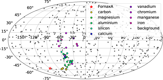
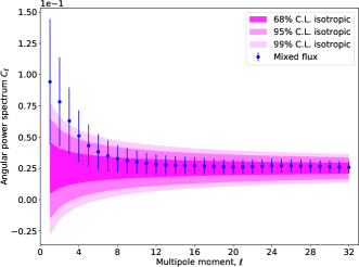
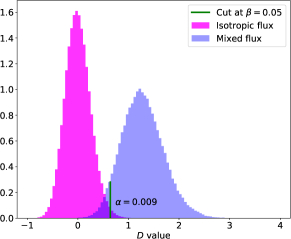
Figure 6: The case of $N_{\mathrm{UHECR}}=500$ and 8% events coming from Fornax A. See the caption of Fig. 2 for other details.

Values of $\alpha$ are sensitive to the fraction of from-source events in samples with $N_{\mathrm{UHECR}}\gtrsim 300$, so that increasing their fraction by one percent can reduce $\alpha$ by almost an order of magnitude. This is especially pronounced for $N_{\mathrm{UHECR}}=500$. For example, increasing the percentage of events coming from NGC 253 up to 8% for $N_{\mathrm{UHECR}}=500$ cuts down $\alpha$ from $0.010$ down to $\approx 5\times 10^{-4}$.

As was mentioned above, all presented results were obtained for $\ell_{\mathrm{max}}=16$ for the sake of uniformity of the analysis. This does not mean this is an optimal value for detecting a deviation from isotropic expectations in each particular case since the behaviour of the $C_{\ell}$ coefficients in the angular power spectrum is specific for every source. The sensitivity of the estimator $D$ in Eq. (1.4) to deviations from isotropy depends on the behaviour of $C_{\ell}$ in each case. For example, the first kind error drops down to $\sim 10^{-4}$ if one takes $\ell_{\mathrm{max}}=6$ for Cen A with $N_{\mathrm{UHECR}}=300$. On the other hand, it is advised to increase $\ell_{\mathrm{max}}$ slightly for M82 in order to obtain smaller $\alpha$ due to a much slower decrease of the $C_{\ell}$ coefficients for this AGN, compare the left bottom panels in Figs. 3 and 4.

It can be seen from Table 1 that the threshold value for the contribution from a single source that can be still detected with a high confidence level is around 10–15% for $N_{\mathrm{UHECR}}\gtrsim 300$, and it does not considerably depend either on the source position on the celestial sphere or on the distance to it. Thus, this value can be straightforwardly compared with theoretical expectations. We used the simplest model of identical sources uniformly distributed with a number density $n$. Given that the characteristic path length $L_{c}$ at the relevant energies is around 100 Mpc (see Fig. 1), we have performed our simulations in a $V_{\mathrm{box}}=(600~{}\mathrm{Mpc})^{3}$ box centered at the observer position. Less than 5% of the total flux comes from outside this box, so we have ignored that part. The total number of simulated sources was equal to $N_{\mathrm{src}}=nV_{\mathrm{box}}$. The contribution from an individual source located at a distance $d$ was calculated as

$$\Phi=\exp(-d/L_{c})/d^{2}.$$

Finally, all contributions were summed up, and fractions of CRs from the brightest (the closest in this set up) and the second-brightest sources were calculated. This procedure was repeated 100,000 times and that gave a fairly good sampling of the distributions (see Fig. 7). The median values of these distributions for different values of density $n$ are presented in Table 3. It can be seen that the analysis of a large-scale anisotropy observed by K-EUSO will have a potential to constrain the density of identically distributed sources at the level $n>(1-2)\times 10^{-5}~{}\mathrm{Mpc^{-3}}$. This value should be compared with the current limits coming from the non-observation of significant clustering at intermediate angular scales in the same energy range by the Pierre Auger Observatory: $n>6\times 10^{-6}~{}\mathrm{Mpc^{-3}}$ [51].

Table 3: Percentage of UHECRs with $E>57$ EeV arriving from the closest and the second closest source in the setup of identical uniformly distributed sources with density $n$.

$n,\mathrm{Mpc}^{-3}$	Closest	Second closest
$10^{-4}$	5.2	1.8
$3\times 10^{-5}$	7.5	2.7
$10^{-5}$	10.6	3.9
$3\times 10^{-6}$	15.0	5.0
$10^{-6}$	20.9	6.3

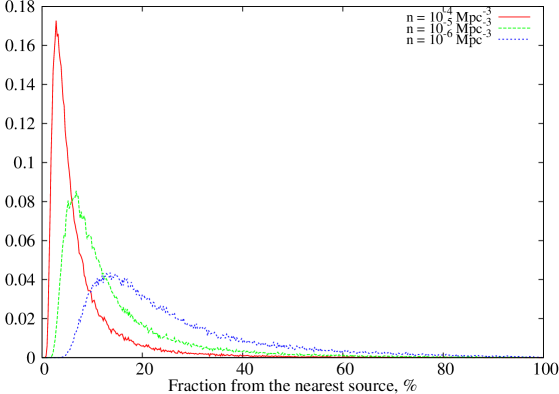
Figure 7: Distribution of contributions of the closest source in the total UHECR flux for different values of the source density $n=10^{-4},\,10^{-5},\,10^{-6}$ Mpc^-3.

3 Anisotropy at lower energies

It was suggested by Lemoine and Waxman [52] that if anisotropy is found above some energy $E$ and the composition is assumed to be heavy at that energy (with nuclei of charge $Z$), one should also observe an even stronger anisotropy at energies above rigidity $E/Z$ due to the proton component of the flux emitted by the source that is responsible for the observed anisotropy. The statement was based on an assumption that the cosmic ray injection spectrum at the source depends on rigidity only.

The idea was further developed in [53]. It was argued in particular that if anisotropy is detected at energies above $\sim 60$ EeV and is caused by heavy nuclei, then an even more significant anisotropy signal should be present at energies close to the ankle due to the proton component. The authors have also considered a case when protons are not injected by the source. It was argued that an anisotropy pattern may then occur at lower energies due to the secondary proton signal produced by photodisintegration of heavy nuclei. However, the significance of an anisotropy predicted in this case at lower energies is weaker than at higher ones unless the nearest source is distant enough (typically beyond $30$ Mpc) and the maximal cosmic ray injection energy $E_{\rm max}\gtrsim Z/26\times 10^{3}$ EeV (see Fig. 2 in [53]).

The composition of UHECRs with energies above 57 EeV arriving at Earth in the KKOS model is comparatively heavy, with $Z\geq 4$. It can be seen in the left panel of Fig. 1 that the primary proton flux is strongly suppressed above $\sim 3$ EeV in the injection spectrum of the model. It might be interesting to estimate if any large-scale anisotropy can be observed at around the ankle of the CR energy spectrum due to the secondary proton component present there, even though this is below the energy threshold of the K-EUSO experiment, and an analysis of the original idea by Lemoine and Waxman performed by Pierre Auger Collaboration did not reveal any overdensities at lower energies in the regions where anisotropies were found for energies above 55 EeV [54].

To address the question, we first evaluated how the fraction of from-source events in the total flux scales with energy. The dependence of the fraction $F_{1}/F_{\mathrm{tot}}$ of cosmic rays arriving from a single source in the total incoming flux on the minimal energy $E_{\mathrm{min}}$ for distances $d=3.5$ Mpc and 20 Mpc is shown in Fig. 8. For definiteness, the flux of UHECRs arriving from a source is normalized in the figure so that $F_{1}/F_{\mathrm{tot}}=10\%$ for $E_{\mathrm{min}}=57$ EeV. The fraction grows with energy since cosmic ray attenuation length drops with increasing $E$.

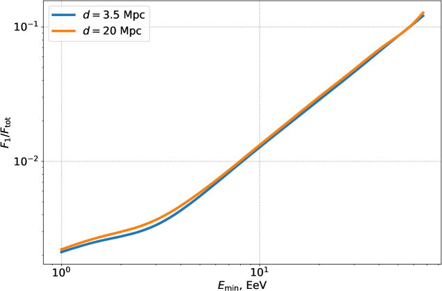
Figure 8: Dependence of the fraction of the flux $F_{1}$ coming from a single source located at the given distance from the observer (3.5 Mpc and 20 Mpc) in the total incoming flux $F_{\text{tot}}$ above some energy threshold $E_{\mathrm{min}}$. It is assumed that $F_{1}/F_{\text{tot}}=0.1$ for cosmic rays above $E_{\mathrm{min}}=57$ EeV.

It is clear from Fig. 8 that the fraction of from-source events scales nearly linearly for $E_{\mathrm{min}}\gtrsim 3$ EeV, and there is very little difference between sources located at distances 3.5 Mpc and 20 Mpc. For both distances, the fraction equals approximately 1% if one considers energies above 8 EeV, which was the threshold value beyond which a dipole anisotropy was detected by the Pierre Auger Collaboration at more than a $5.2\sigma$ level of significance [2]. (The amplitude of the dipole was found to be of $6.5^{+1.3}_{-0.9}$ percent, basing on the analysis of 32,187 events.)

We performed simulations similar to those described above for energies $\geq 8$ EeV to check if a large-scale anisotropy can be found in this energy range assuming it is observed beyond 57 EeV. We considered Cen A and Fornax A as candidates sources because (i) they are located at the opposite ends of the interval of distances, (ii) they demonstrate clearly different patterns of arrival directions of UHECRs due to deflections in the Galactic magnetic field, and (iii) their positions are within the field of view of the Pierre Auger Observatory. The angular power spectra obtained for the two cases are shown in Fig. 9. To make the plots, we simulated 500,000 isotropic samples and 50,000 mixed samples with from-source events comprising 1%, as suggested by Fig. 8. Each sample consisted of 50,000 events, which roughly corresponds to the number of events used with $E\geq 8$ EeV used in the analysis by Auger [2].

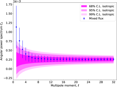
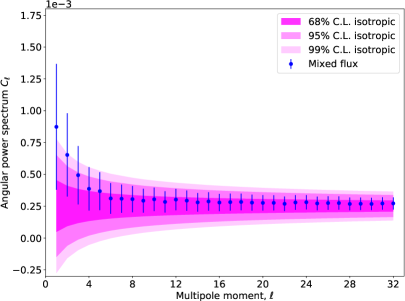
Figure 9: Angular power spectrum $C_{\ell}$ for isotropic and mixed samples arriving from Cen A (left) and Fornax A (right) for cosmic rays above 8 EeV and $F_{1}/F_{\text{tot}}=0.01$. Notation is explained in the caption of Fig. 2.

It can be seen from Fig. 9 that a deviation from the isotropic distribution is less pronounced in this case compared to energies above 57 EeV, cf. Figs. 3 and 6. The first harmonic $C_{1}=(1.1\pm 0.6)\times 10^{-3}$ for Cen A, and $C_{1}=(8.7\pm 4.9)\times 10^{-4}$ in the case of Fornax A. Since the dipole amplitude can be estimated as $\sqrt{9C_{1}/4\pi}$ (see, e.g., [55]), this immediately gives dipoles of 2.9% and 2.5% respectively, approximately 2.2–2.6 times less than the dipole found by Auger [2]. An estimation obtained the same way in [49] with approximately 20,000 events gave an amplitude of the dipole equal to $(6.0\pm 1.5)\%$, thus more than two times greater than those of ours.

The result qualitatively agrees with one of the conclusions of [42] that the dipole amplitude increases at higher energies. It also explains why a dipole anisotropy near the ankle in the CR energy spectrum associated with a nearby source has not been detected by the current experiments assuming such an anisotropy exists at energies beyond 57 EeV.

4 Conclusions

We have studied if the future K-EUSO orbital detector will be able to observe possible signatures of a large-scale anisotropy of ultra-high-energy cosmic rays above 57 EeV arising in the minimal model for extragalactic CRs and neutrinos [19], a self-consistent scenario attributing the origin of UHECRs and high energy neutrinos to (possibly a subclass of) AGN. We considered five possible candidate sources often discussed in literature and allowed by the model (Centaurus A, M82, NGC 253, M87 and Fornax A), focusing on the case of a single source providing a deviation from an otherwise isotropic distribution. Using extensive simulations performed with the publicly available, open-source TransportCR and CRPropa 3 packages, we explored how anisotropies depend on the energy threshold, the number of registered UHECRs and the fraction of from-source events in the whole sample. We demonstrate that an observation of $\gtrsim 300$ events above 57 EeV will allow detecting a large-scale anisotropy with a high confidence level providing the fraction of from-source events is $\simeq$10–15%, depending on a particular source, with a smaller source contribution for larger samples. We also show that anisotropy signatures originating from the same nearby sources are not expected to be strong at the ankle region in the KKOS model, which assumes a heavy UHECR composition at the highest energies.

The presented results are generic and can be applied to other future experiments with a full-sky coverage and a uniform exposure, including the planned POEMMA mission [40].

References

- [1] J. Linsley, L. Scarsi and B. Rossi, Extremely energetic cosmic-ray event, Physical Review Letters 6 (May, 1961) 485–487.
- [2] Pierre Auger Collaboration, A. Aab, P. Abreu, M. Aglietta, I. A. Samarai, I. F. M. Albuquerque et al., Observation of a large-scale anisotropy in the arrival directions of cosmic rays above eV, Science 357 (Sept., 2017) 1266–1270, [1709.07321].
- [3] E. Waxman, Cosmological gamma-ray bursts and the highest energy cosmic rays, Phys. Rev. Lett. 75 (Jul, 1995) 386–389.
- [4] M. Milgrom and V. Usov, Possible association of ultra-high-energy cosmic-ray events with strong gamma-ray bursts, The Astrophysical Journal Letters 449 (Aug., 1995) L37, [astro-ph/9505009].
- [5] M. Vietri, The acceleration of ultra–high-energy cosmic rays in gamma-ray bursts, Astrophysical Journal 453 (Nov., 1995) 883, [astro-ph/9506081].
- [6] P. Blasi, R. I. Epstein and A. V. Olinto, Ultra-high-energy cosmic rays from young neutron star winds, The Astrophysical Journal Letters 533 (Apr., 2000) L123–L126, [astro-ph/9912240].
- [7] J. Arons, Magnetars in the metagalaxy: An origin for ultra-high-energy cosmic rays in the nearby universe, Astrophysical Journal 589 (June, 2003) 871–892, [astro-ph/0208444].
- [8] K. Fang, K. Kotera and A. V. Olinto, Newly born pulsars as sources of ultrahigh energy cosmic rays, Astrophysical Journal 750 (May, 2012) 118, [1201.5197].
- [9] G. R. Farrar and A. Gruzinov, Giant AGN flares and cosmic ray bursts, Astrophysical Journal 693 (Mar., 2009) 329–332, [0802.1074].
- [10] G. R. Farrar, Tidal disruption flares as the source of ultra-high energy cosmic rays, in European Physical Journal Web of Conferences, vol. 39 of European Physical Journal Web of Conferences, p. 07005, Dec., 2012, 1210.1232, DOI.
- [11] C. Guépin, K. Kotera, E. Barausse, K. Fang and K. Murase, Ultra-high-energy cosmic rays and neutrinos from tidal disruptions by massive black holes, Astronomy & Astrophysics 616 (Sept., 2018) A179, [1711.11274].
- [12] A. Pe’er, K. Murase and P. Mészáros, Radio-quiet active galactic nuclei as possible sources of ultrahigh-energy cosmic rays, Physical Review D 80 (Dec., 2009) 123018, [0911.1776].
- [13] K. Murase, C. D. Dermer, H. Takami and G. Migliori, Blazars as ultra-high-energy cosmic-ray sources: Implications for TeV gamma-ray observations, Astrophysical Journal 749 (Apr., 2012) 63, [1107.5576].
- [14] B. A. Nizamov and M. S. Pshirkov, Constraints on the AGN flares as sources of ultra-high energy cosmic rays from the Fermi-LAT observations, arXiv e-prints (Apr, 2018) arXiv:1804.01064, [1804.01064].
- [15] C. D. Dermer, S. Razzaque, J. D. Finke and A. Atoyan, Ultra-high-energy cosmic rays from black hole jets of radio galaxies, New Journal of Physics 11 (June, 2009) 065016, [0811.1160].
- [16] K. Fang and K. Murase, Linking high-energy cosmic particles by black-hole jets embedded in large-scale structures, Nature Physics 14 (Apr., 2018) 396–398, [1704.00015].
- [17] S. S. Kimura, K. Murase and B. T. Zhang, Ultrahigh-energy cosmic-ray nuclei from black hole jets: Recycling galactic cosmic rays through shear acceleration, Physical Review D 97 (Jan., 2018) 023026, [1705.05027].
- [18] K. Kotera and A. V. Olinto, The astrophysics of ultrahigh-energy cosmic rays, Annu. Rev. Astron. Astrophys. 49 (Sept., 2011) 119–153, [1101.4256].
- [19] M. Kachelrieß, O. Kalashev, S. Ostapchenko and D. V. Semikoz, Minimal model for extragalactic cosmic rays and neutrinos, Phys. Rev. D96 (2017) 083006, [1704.06893].
- [20] D. Kazanas and D. C. Ellison, The central engine of quasars and active galactic nuclei: Hadronic interactions of shock-accelerated relativistic protons, Astrophys. J. 304 (May, 1986) 178–187.
- [21] R. D. Blandford, Accretion disc electrodynamics—a model for double radio sources, Monthly Notices of the Royal Astronomical Society 176 (1976) 465–481.
- [22] R. V. E. Lovelace, Dynamo model of double radio sources, Nature 262 (Aug, 1976) 649–652.
- [23] R. D. Blandford and R. L. Znajek, Electromagnetic extractions of energy from Kerr black holes, Mon. Not. Roy. Astron. Soc. 179 (1977) 433–456.
- [24] D. MacDonald and K. S. Thorne, Black-hole electrodynamics: an absolute-space/universal-time formulation, Mon. Not. Roy. Astron. Soc. 198 (1982) 345–382.
- [25] A. Y. Neronov, D. V. Semikoz and I. I. Tkachev, Ultra-high energy cosmic ray production in the polar cap regions of black hole magnetospheres, New J. Phys. 11 (2009) 065015, [0712.1737].
- [26] J. P. Rachen and P. L. Biermann, Extragalactic ultrahigh-energy cosmic rays. 1. Contribution from hot spots in FR-II radio galaxies, Astron. Astrophys. 272 (1993) 161–175, [astro-ph/9301010].
- [27] M. J. Hardcastle, C. C. Cheung, I. J. Feain and L. Stawarz, High-energy particle acceleration and production of ultra-high-energy cosmic rays in the giant lobes of Centaurus A, Mon. Not. Roy. Astron. Soc. 393 (2009) 1041–1053, [0808.1593].
- [28] IceCube collaboration, M. G. Aartsen et al., Observation and characterization of a cosmic muon neutrino flux from the northern hemisphere using six years of IceCube data, Astrophys. J. 833 (2016) 3, [1607.08006].
- [29] Fermi-LAT collaboration, M. Ackermann et al., The spectrum of isotropic diffuse gamma-ray emission between 100 MeV and 820 GeV, Astrophys. J. 799 (2015) 86, [1410.3696].
- [30] B. Rouillé d’Orfeuil, D. Allard, C. Lachaud, E. Parizot, C. Blaksley and S. Nagataki, Anisotropy expectations for ultra-high-energy cosmic rays with future high-statistics experiments, Astronomy & Astrophysics 567 (July, 2014) A81, [1401.1119].
- [31] F. Oikonomou, K. Kotera and F. B. Abdalla, Simulations for a next-generation UHECR observatory, Journal of Cosmology and Astroparticle Physics 1 (Jan., 2015) 030, [1409.1925].
- [32] P. B. Denton and T. J. Weiler, Sensitivity of full-sky experiments to large scale cosmic ray anisotropies, Journal of High Energy Astrophysics 8 (Dec., 2015) 1–9, [1505.03922].
- [33] G. K. Garipov, M. Y. Zotov, P. A. Klimov, M. I. Panasyuk, O. A. Saprykin, L. G. Tkachev et al., The KLYPVE ultra high energy cosmic ray detector on board the ISS, Bull. Rus. Acad. Sci. Physics 79 (2015) 326–328.
- [34] M. Panasyuk, P. Klimov, B. Khrenov, S. Sharakin, M. Zotov, P. Picozza et al., Ultra high energy cosmic ray detector KLYPVE on board the Russian Segment of the ISS, in 34th International Cosmic Ray Conference (ICRC2015), vol. 34, p. 669, July, 2015, https://pos.sissa.it/236/669/pdf.
- [35] P. Klimov, M. Casolino and the JEM-EUSO Collaboration, Status of the KLYPVE-EUSO detector for EECR study on board the ISS, in Proceedings, 35th International Cosmic Ray Conference (ICRC 2017): Bexco, Busan, Korea, July 12-20, 2017, p. 412, 2017, https://pos.sissa.it/301/412/pdf.
- [36] M. Casolino, A. Belov, M. Bertaina, T. Ebisuzaki and the JEM-EUSO Collaboration, KLYPVE-EUSO: science and UHECR observational capabilities, in Proceedings, 35th International Cosmic Ray Conference (ICRC 2017): Bexco, Busan, Korea, July 12-20, 2017, p. 368, 2017, https://pos.sissa.it/301/368/pdf.
- [37] P. A. Klimov, M. I. Panasyuk, B. A. Khrenov, G. K. Garipov, N. N. Kalmykov, V. L. Petrov et al., The TUS detector of extreme energy cosmic rays on board the Lomonosov satellite, Space Science Reviews 212 (Aug, 2017) 1687–1703, [1706.04976].
- [38] B. A. Khrenov, P. A. Klimov, M. I. Panasyuk, S. A. Sharakin, L. G. Tkachev, M. Y. Zotov et al., First results from the TUS orbital detector in the extensive air shower mode, Journal of Cosmology and Astroparticle Physics 2017 (2017) 006, [1704.07704].
- [39] D. Semikoz, P. Tinyakov and M. Zotov, Detection prospects of the Telescope Array hotspot by space observatories, Phys. Rev. D93 (2016) 103005, [1601.06363].
- [40] A. V. Olinto, J. H. Adams, R. Aloisio, L. A. Anchordoqui, D. R. Bergman, M. E. Bertaina et al., POEMMA: Probe Of Extreme Multi-Messenger Astrophysics, in Proceedings, 35th International Cosmic Ray Conference (ICRC 2017): Bexco, Busan, Korea, July 12-20, 2017, vol. 301, p. 542, 2017, 1708.07599.
- [41] D. Harari, S. Mollerach and E. Roulet, Angular distribution of cosmic rays from an individual source in a turbulent magnetic field, Physical Review D 93 (Mar, 2016) 063002, [1512.08289].
- [42] A. Dundović and G. Sigl, Anisotropies of ultra-high energy cosmic rays dominated by a single source in the presence of deflections, Journal of Cosmology and Astro-Particle Physics 2019 (Jan, 2019) 018, [1710.05517].
- [43] O. E. Kalashev and E. Kido, Simulations of ultra high energy cosmic rays propagation, J. Exp. Theor. Phys. 120 (2015) 790–797, [1406.0735].
- [44] R. Alves Batista, A. Dundovic, M. Erdmann, K.-H. Kampert, D. Kuempel, G. Müller et al., CRPropa 3—a public astrophysical simulation framework for propagating extraterrestrial ultra-high energy particles, Journal of Cosmology and Astroparticle Physics 1605 (2016) 038, [1603.07142].
- [45] R. Jansson and G. R. Farrar, A new model of the Galactic magnetic field, Astrophys. J. 757 (Sept., 2012) 14, [1204.3662].
- [46] P. Sommers, Cosmic ray anisotropy analysis with a full-sky observatory, Astroparticle Physics 14 (Jan, 2001) 271–286, [astro-ph/0004016].
- [47] O. Deligny, E. Armengaud, T. Beau, P. Da Silva, J.-C. Hamilton, C. Lachaud et al., Angular power spectrum estimation of cosmic ray anisotropies with full or partial sky coverage, Journal of Cosmology and Astroparticle Physics 10 (Oct., 2004) 008, [astro-ph/0404253].
- [48] J. Hülss and C. Wiebusch, Search for signatures of extra-terrestrial neutrinos with a multipole analysis of the AMANDA-II sky-map, in Proceedings, 30th International Cosmic Ray Conference (ICRC 2007): Merida, Mexico, July 3–11 2007, 2007, 0711.0353.
- [49] Pierre Auger collaboration, A. Aab et al., Multi-resolution anisotropy studies of ultrahigh-energy cosmic rays detected at the Pierre Auger Observatory, Journal of Cosmology and Astroparticle Physics 1706 (2017) 026, [1611.06812].
- [50] S. van Velzen, H. Falcke, P. Schellart, N. Nierstenhöfer and K.-H. Kampert, Radio galaxies of the local universe. All-sky catalog, luminosity functions, and clustering, Astronomy & Astrophysics 544 (Aug., 2012) A18, [1206.0031].
- [51] Pierre Auger Collaboration, Bounds on the density of sources of ultra-high energy cosmic rays from the Pierre Auger Observatory, Journal of Cosmology and Astroparticle Physics 5 (May, 2013) 009, [1305.1576].
- [52] M. Lemoine and E. Waxman, Anisotropy vs chemical composition at ultra-high energies, Journal of Cosmology and Astroparticle Physics 2009 (Nov., 2009) 009, [0907.1354].
- [53] R.-Y. Liu, A. M. Taylor, M. Lemoine, X.-Y. Wang and E. Waxman, Constraints on the source of ultra-high-energy cosmic rays using anisotropy versus chemical composition, Astrophysical Journal 776 (Oct., 2013) 88, [1308.5699].
- [54] Pierre Auger Collaboration, P. Abreu, M. Aglietta, E. J. Ahn et al., Anisotropy and chemical composition of ultra-high energy cosmic rays using arrival directions measured by the Pierre Auger Observatory, Journal of Cosmology and Astroparticle Physics 2011 (June, 2011) 022, [1106.3048].
- [55] C. Gibelyou and D. Huterer, Dipoles in the sky, Monthly Notices of the Royal Astronomical Society 427 (Dec, 2012) 1994–2021, [1205.6476].
- [56] M. Wenger, F. Ochsenbein, D. Egret, P. Dubois, F. Bonnarel, S. Borde et al., The SIMBAD astronomical database. The CDS reference database for astronomical objects, Astronomy and Astrophysics Supplement 143 (Apr., 2000) 9–22, [astro-ph/0002110].
- [57] F. Pérez and B. E. Granger, IPython: a system for interactive scientific computing, Computing in Science and Engineering 9 (May, 2007) 21–29.
- [58] J. D. Hunter, Matplotlib: A 2d graphics environment, Computing In Science & Engineering 9 (2007) 90–95.
- [59] K. M. Górski, E. Hivon, A. J. Banday, B. D. Wandelt, F. K. Hansen, M. Reinecke et al., HEALPix: A framework for high-resolution discretization and fast analysis of data distributed on the sphere, Astrophys. J. 622 (Apr., 2005) 759–771, [astro-ph/0409513].