Thermoelectric properties of gapped bilayer graphene

Abstract

Unlike in conventional semiconductors, both the chemical potential and the band gap in bilayer graphene (BLG) can be tuned via application of external electric field. Among numerous device implications, this property also designates BLG as a candidate for high-performance thermoelectric material. In this theoretical study we have calculated the Seebeck coefficients for abrupt interface separating weakly- and heavily-doped areas in BLG, and for a more realistic rectangular sample of mesoscopic size, contacted by two electrodes. For a given band gap ($\Delta$) and temperature ($T$) the maximal Seebeck coefficient is close to the Goldsmid-Sharp value $|S|_{\rm max}^{\rm GS}=\Delta/(2eT)$, the deviations can be approximated by the asymptotic expression $|S|_{\rm max}^{\rm GS}-|S|_{\rm max}=(k_{B}/e)\times\left[\frac{1}{2}\ln{u}+\ln{}2-\frac{1}{2}+{\cal O}(u^{-1})\right]$, with the electron charge $-e$, the Boltzmann constant $k_{B}$, and $u=\Delta/(2k_{B}T)\gg{}1$. Surprisingly, the effects of trigonal warping term in the BLG low-energy Hamiltonian are clearly visible at few-Kelvin temperatures, for all accessible values of $\Delta\leqslant{}300\,$meV. We also show that thermoelectric figure of merit is noticeably enhanced ($ZT>3$) when a rigid substrate suppresses out-of-plane vibrations, reducing the contribution from ZA phonons to the thermal conductivity.

I Introduction

In recent years, bilayer graphene (BLG) devices made it possible to demonstrate several intriguing physical phenomena, including the emergence of quantum spin Hall phase Qia11 ; Mah13 , the fractal energy spectrum known as Hofstadter’s butterfly Dea13 ; Pon13 , or unconventional superconductivity Cao18a ; Cao18b , just to mention a few. From a bit more practical perspective, a number of plasmonic and photonic instruments were designed and build Yan09 ; Bon10 ; Gri12 constituting platforms for application considerations. BLG-based thermoelectric devices have also attracted a significant attention Wan11 ; Chi16 ; Mah17 ; Sus18 , next to the devices based on other two-dimensional (2D) materials Lee16 ; Sev17 ; Qin18 .

In a search for high-performance thermoelectric material, one’s attention usually focusses on enhancing the dimensionless figure of merit Mah95 ; Kim15

$$ZT=\frac{GS^{2}T}{K},$$ (1)

where $G$, $S$ and $K$ are (respectively): the electrical conductance, the Seebeck coefficient quantifying the thermopower, and the thermal conductance; the last characteristic can be represented as $K=K_{\rm el}+K_{\rm ph}$, with $K_{\rm el}$ ($K_{\rm ph}$) being the electronic (phononic) part. This is because the maximal energy conversion efficiency is related to $ZT$ via Iof57

$$\eta_{\rm max}=\frac{\Delta{}T}{T_{h}}\frac{\sqrt{1+ZT_{\rm av}}-1}{\sqrt{1+ZT_{\rm av}}+\frac{T_{c}}{T_{h}}},$$ (2)

where $T_{c}$ ($T_{h}$) is the hot- (or cool) side temperature, $\Delta{}T=T_{h}-T_{c}$, and $T_{\rm av}=(T_{c}+T_{h})/2$. In particular, for $ZT_{\rm av}=3$ we have $\eta_{\rm max}>\frac{1}{3}\Delta{}T/T_{h}$ (with $\Delta{}T/T_{h}$ the Carnot efficiency), and therefore $ZT>3$ is usually regarded as a condition for thermoelectric device to be competitive with other power generation systems.

As the Seebeck coefficient is squared in Eq. (1), a maximum of $ZT$ — considered as a function of the driving parameters specified below — is commonly expected to appear close to a maximum of $|S|$. Here we show this is not always the case in gapped BLG: when discussing in-plane thermoelectric transport in a presence of perpendicular electric field such that the band gap is much greater than the energy of thermal excitations ($\Delta\gg{}k_{B}T$), the maximal absolute thermopower $|S|_{\rm max}$ corresponds to the electrochemical potential relatively close to the center of a gap, namely $\mu_{\rm max}^{|S|}\approx{}\pm\frac{1}{2}k_{B}T\ln(2\Delta/k_{B}T)$, whereas the maximal figure of merit $ZT_{\rm max}$ appears near the maximum of the valence band (or the minimum of the conduction band), i.e., $\mu_{\rm max}^{ZT}\approx{}\pm\Delta/2$. In contrast to $ZT_{\rm max}$, $|S|_{\rm max}$ is not directly related to the value of the transmission probability near the band boundary, and these two quantities show strikingly different behaviors with increasing $\Delta$ for a given $T$.

Qualitatively, one can expect that thermoelectric performance of BLG is enhanced with increasing $\Delta$, since abrupt switching behavior is predicted for the conductance $G$ when passing $\mu=\pm{}\Delta/2$ for $\Delta\gg{}k_{B}T$ Cut69 ; Rut14b . (Moreover, the gap opening suppresses $\kappa_{\rm el}$, reducing the denominator in Eq. (1).) Such a common intuition is build on the Mott formula, according to which $S$ is proportional to the logarithmic derivative of $G$ as a function of the Fermi energy $E_{F}$. One cannot, however, directly apply the Mott formula for gapped systems at nonzero temperatures, and the link between a rapid increase of $G(E_{F})$ for $E_{F}\approx{}\Delta/2$ and high $|S|$ is thus not direct in the case of gapped BLG, resulting in $\mu_{\rm max}^{|S|}\ll{}\Delta/2$.

The results of earlier numerical work Hao10 suggest that $|S|_{\rm max}$, obtained by adjusting $\mu$ for a given $\Delta$ and $T$, is close to

$$|S|_{\rm max}^{\rm GS}=\frac{\Delta}{2eT},$$ (3)

being the Goldsmid-Sharp value for wide-gap semiconductors Gol99 . In this paper, we employ the Landauer-Büttiker approach for relatively large ballistic BLG samples, finding that Eq. (3) provides a reasonable approximation of the actual $|S|_{\rm max}$ for $\Delta\sim{}k_{B}{}T$ only. For larger $\Delta$, a logarithmic correction becomes significant, and the deviation exceeds $k_{B}/e$ ($\approx{}86\,\mu$V/K) for $\Delta\gtrsim{}10\,k_{B}{}T$. We further find that—although $|S|_{\rm max}$ grows monotonically when increasing $\Delta$ at fixed $T$ and may reach (in principle) arbitrarily large value—$ZT_{\rm max}$ shows a conditional maximum at $\Delta_{\star}(T)\sim{}10^{2}\,k_{B}{}T$ (for $T\leqslant{}10\,$K). An explanation of these findings in terms of a simplified model for transmission-energy dependence is provided.

II Model and methods

The two systems considered are shown schematically in Figs. 1(a) and 1(b). The first system (hereinafter called an abrupt interface) clearly represents an idealized case, as we have supposed that both the doping and temperature change rapidly on the length-scale much smaller than the Fermi wavelength for an electron. Therefore, a comparison with the second system, in which chemical potentials and temperatures are attributed to macroscopic reservoirs (the two leads), separated by a sample area of a finite length $L$, is essential to validate the applicability of our precictions for real experiments.

We take the four-band Hamiltonian for BLG Mac13

$$H=\xi\left(\begin{array}[]{cccc}-U/2&v_{F}\pi&\xi{}t_{\perp}&0\\ v_{F}\pi^{\dagger}&-U/2&0&v_{3}\pi\\ \xi{}t_{\perp}&0&U/2&v_{F}\pi^{\dagger}\\ 0&v_{3}\pi^{\dagger}&v_{F}\pi&U/2\end{array}\right),$$ (4)

where the valley index $\xi=1$ for $K$ valley or $\xi=-1$ for $K^{\prime}$ valley, $\pi=p_{x}+ip_{y}$, $\pi^{\dagger}=p_{x}-ip_{y}$, with $\mbox{\boldmath$p$}=(p_{x},p_{y})$ the carrier momentum, $v_{F}=\sqrt{3}at_{0}/(2\hbar)$ is the Fermi velocity, $v_{3}=(t^{\prime}/t_{0})v_{F}$, $U$ is the electrostatic bias between the layers, and $a=0.246\,$nm is the lattice parameter. Following Ref. Kuz09 , we set $t_{0}=3.16\,$eV – the nearest-neighbor in-plane hopping energy, $t_{\perp}=0.381\,$eV – the direct interlayer hopping energy; the skew interlayer hopping energy is set as $t^{\prime}=0$ or $t^{\prime}=0.3\,$eV in order to discuss the role of trigonal warping fig1foo . The band gap $\Delta\approx{}|U|$ for $|U|\ll{}t_{\perp}$ and $t^{\prime}=0$ (remaining details are given in Supplementary Information, Sec. I). Solutions of the subsequent Dirac equation, $H\Psi=E\Psi$, with $\Psi=(\Psi_{A1},\Psi_{B1},\Psi_{B2},\Psi_{A2})^{T}$ the probability amplitudes, are matched for the interfaces separating weakly- and heavily-doped regions allowing us to determine the energy-dependent transmission probability $T(E)$ (see Supplementary Information, Sec. II).

At zero temperature, the relation between physical carrier concentration (the doping) and the Fermi energy $E_{F}$ can be approximated by a close-form expression for $t^{\prime}=0$ and $|E_{F}|\!-\!\Delta/2\ll{}t_{\perp}$, namely

$$n(E_{F})\approx{}\frac{t_{\perp}}{\pi{}(\hbar{}v_{F})^{2}}{\rm max}\left(0,|E_{F}|-\Delta/2\right),$$ (5)

following from a piecewise-constant density of states in such a parameter range Mac13 . The prefactor in Eq. (5) $(1/\pi)\,t_{\perp}/(\hbar{}v_{F})^{2}\approx 0.268\,$nm^-2eV^-1 . In a general situation, it is necessary to perform the numerical integration of the density of states following from the Hamiltonian $H$ (4) (see Supplementary Information, Sec. I); however, Eq. (5) gives a correct order of magnitude for $\Delta\gg{}k_{B}{}T$. In the remaining part of the paper, we discuss thermoelectric characteristics as functions of the electrochemical potential $\mu$, keeping in mind that the doping $n=n(|\mu|)$ is a monotonically increasing function of $|\mu|$.

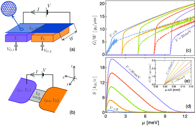
Figure 1: Systems studied numerically in the paper (left) and their basic thermoelectric characteristics (right). (a) BLG strip of width $W$ with a voltage source driving electric current through the strip. Two gate electrodes, with different temperatures $T_{1}$ and $T_{2}$, induce an abrupt interface (dash-dot line) between the weakly-doped (light area) and the heavily-doped (dark area) regions. (b) A finite, weakly-doped section of the strip (of length $L$) with leads driving both thermal and electric currents. In both cases, additional gate electrodes (not shown) allow to tune the electrostatic bias between the layers (see Ref. fig1foo ). The coordinate system is also shown. (c) Zero-temperature conductance, specified in the units of $g_{0}=4e^{2}/h$, and (d) the Seebeck coefficient at $T=5\,$K as functions of the chemical potential. Solid lines correspond to the system of panel (a), dashed lines correspond to the system of panel (b). (e) Zoom-in of the conductance as a function of the chemical potential measures from the conduction band minimum ($\mu=\Delta/2$) for the system of panel (a). Skew-interlayer hopping is fixed at $t^{\prime}=0.3\,$eV. The electrostatic bias between the layers is varied from $U=0$ to $U=20\,$meV in steps of $5\,$meV (c,d) or from $U=10\,$meV to $U=150\,$meV in steps of $20\,$meV (e). (The extreme values of $U$ are specified for corresponding lines.)

Next, we employ the Landauer-Büttiker expressions for the electrical and thermal currents Lan57 ; But85

$$I =-\frac{g_{s}g_{v}e}{h}\int{}dE\,T(E)\left[f_{L}(E)\!-\!f_{R}(E)\right],$$ (6)

$$I_{Q} =\frac{g_{s}g_{v}}{h}\int{}dE\,T(E)\left[f_{L}(E)\!-\!f_{R}(E)\right](E\!-\!\mu),$$ (7)

where $g_{s}=g_{v}=2$ are spin and valley degeneracies, $f_{L}$ and $f_{R}$ are the distribution functions for the left and right reservoirs, with their electrochemical potentials $\mu_{L}$ and $\mu_{R}$, and temperatures $T_{L}$ and $T_{R}$. We further suppose that $\mu_{L}-\mu_{R}\equiv{}-eV$ and $T_{L}-T_{R}\equiv{}\Delta{}T$ are infinitesimally small (the linear-response regime) and define $\mu=(\mu_{L}+\mu_{R})/2$ and $T=(T_{L}+T_{R})/2$. The conductance $G$, the Seebeck coefficient $S$, and the electronic part of the thermal conductance $K_{\rm el}$, are given by Esf06

$$G =\left.\frac{I}{V}\right|_{\Delta{}T=0}=e^{2}L_{0},$$ (8)

$$S =-\left.\frac{V}{\Delta{}T}\right|_{I=0}=\frac{L_{1}}{eTL_{0}},$$ (9)

$$K_{\rm el} =\left.\frac{I_{Q}}{\Delta{}T}\right|_{I=0}=\frac{L_{0}L_{2}-L_{1}^{2}}{TL_{0}},$$ (10)

where

$$L_{n} =\frac{g_{s}g_{v}}{h}\int{}dE\,T(E)\left(-\frac{\partial{}f_{\rm FD}}{\partial{}E}\right)(E-\mu)^{n}$$

$$(n=0,1,2)$$ (11)

with $f_{\rm FD}(\mu,T,E)=1/\left[\,\exp\left((E\!-\!\mu)/k_{B}T\right)+1\,\right]$ being the Fermi-Dirac distribution function. In particular, for $T\rightarrow{}0$, Eq. (8) reduces to $G=(g_{s}g_{v}e^{2}/h)T(\mu)$, the well-known zero-temperature Landauer conductance.

The phononic part of the thermal conductance, occuring in Eq. (1), can be calculated using

$$K_{\rm ph}=\frac{1}{2\pi}\int{}d\omega\,\hbar{}\omega\frac{\partial{}f_{\rm BE}}{\partial{}T}{\cal T}_{\rm ph}(\omega),$$ (12)

with $f_{\rm BE}(T,\omega)=1/\left[\,\exp\left(\hbar\omega/k_{B}{}T\right)-1\,\right]$ the Bose-Einstein distribution function and ${\cal T}_{\rm ph}(\omega)$ the phononic transmission spectrum. We calculate ${\cal T}_{\rm ph}(\omega)$ by adopting the procedure developed by Alofi and Srivastava Alo13 to the two systems considered in this work (see Supplementary Information, Sec. IV).

III Numerical results

Before discussing the thermoelectric properties in details, we present zero-temperature conductance spectra, which represent the input data to calculate thermoelectric properties (see Sec. II). Since the Hamiltonian given by Eq. (4) is particle-hole symmetric, it is sufficient to limit the discussion to $\mu\geqslant{}0$.

Typically, the conductance $G(\mu)$ of the finite-strip section, compared with the case of an abrupt interface, is reduced by approximately $50\%$ near the conduction band minimum ($\mu=\Delta/2$) due to backscattering on the second interface, and slowly approaches the abrupt-interface limit for $\mu\gg{}\Delta/2$; see Fig. 1(c). Additionally, for a rectangular setup of Fig. 1(b) oscillations of the Fabry-Pérot type are well-pronounces, see Ref. Sus18 . In contrast, the Seebeck coefficient is almost identical for both systems, see Fig. 1(d). We further notice that the conductance near $\mu=\Delta/2$, displayed in Fig. 1(e), is gradually suppressed with increasing $U$. (Hereinafter, the bandgap $\Delta$ is determined numerically for the dispersion relation following from Eq. (4), see Supplementary Information, Sec. I. In general, $\Delta<|U|$ Mac13 ).

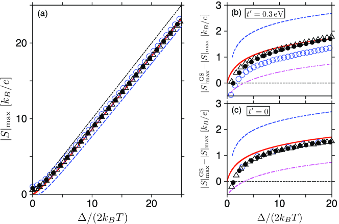
Figure 2: (a) Maximal absolute value of the Seebeck coefficient and (b,c) its deviation from the Goldsmid-Sharp value $|S|_{\rm max}^{{\rm GS}}=\Delta/(2eT)$ calculated numerically for the system of Fig. 1(a) (datapoints) as functions of the energy gap for different temperatures $T=1\,$K (open circles), $T=5\,$K (full circles), and $T=10\,$K (triangles). Skew-interlayer hopping integral is $t^{\prime}=0.3\,$eV (a,b) or $t^{\prime}=0$ (c). Lines depict $S_{\rm max}=S_{\rm max}^{{\rm GS}}$ (black dotted line), and predictions of the model for transmission-energy dependence given by Eq. (III) with $\alpha=0$ (blue dashed line), $\alpha=1$ (red solid line), and $\alpha=2$ (magenta dash-dot line — omitted in panel (a) for clarity).

The close overlap of the thermopower spectra presented in Fig. 1(d) allows us to limit the discussion of $|S|_{\rm max}$ to the case of an abrupt interface, see Figs. 2(a), 2(b), and 2(c). In order to rationalize the deviations of the numerical data from $|S|_{\rm max}^{\rm GS}$ given by Eq. (3), we propose a family of models for the transmission-energy dependence, namely

$$T^{(\alpha)}={\cal C}(\Delta)\times\begin{cases}\delta(E-\frac{1}{2}\Delta)+\delta(E+\frac{1}{2}\Delta)&\text{if }\alpha=0\\ \Theta(|E|-\frac{1}{2}\Delta)(|E|-\frac{1}{2}\Delta)^{\alpha-1}&\text{if }\alpha>0\end{cases}$$ (13)

with the prefactor ${\cal C}(\Delta)$ quantifying the transmission propability near the band boundary $|E|\approx\frac{1}{2}\Delta$, $\delta(x)$ being the Dirac delta function, and $\Theta(x)$ being the Heaviside step function. The analytic expressions presented here, and later in Sec. IV, are (unless otherwise specified) valid for any $\alpha\geqslant{}0$, althought when comparing model predictions with the numerical data we limit our considerations to integer $\alpha$.

In particular, Eq. (13) leads to the maximal absolute value of the Seebeck coefficient

$$|S|_{\rm max}^{(\alpha)}\times\left({k_{B}}/{e}\right)^{-1} \approx\sqrt{(u+\alpha)(u+\alpha-1)}-\ln\left(\sqrt{u+\alpha}+\sqrt{u+\alpha-1}\right)$$

$$=u-\frac{1}{2}\ln{}\left(4u\right)+\alpha-\frac{1}{2}+\frac{3-7\alpha+\alpha^{2}}{8u}+{\cal O}(u^{-2}) \text{for }\alpha\geqslant{}0,$$ (14)

where the first asymptotic equality corresponds to $u=\Delta/(2k_{B}{}T)\gg{}1$ (see Supplementary Information). It is clear from Fig. 2(a) that $|S|_{\rm max}^{(\alpha)}$ with $\alpha=1$ (red solid line) reproduces the actual numerical results (datapoints) noticeably better than $|S|_{\rm max}^{(\alpha)}$ with $\alpha=0$ (blue dashed line) or $|S|_{\rm max}^{\rm GS}$ (black dotted line). What is more, the deviations $|S|_{\rm max}^{\rm GS}-|S|_{\rm max}$, displayed as functions of $\Delta$, allows one to easily identify the effects of trigonal warping, see Fig. 2(b) for $t^{\prime}=0.3\,$eV and Fig. 2(c) for $t^{\prime}=0$.

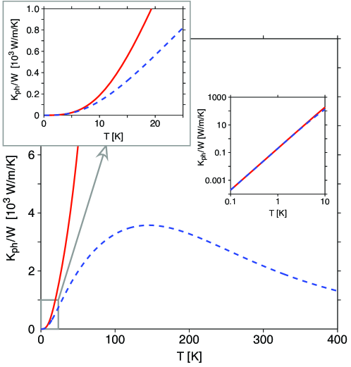
Figure 3: Phononic parts of the thermal conductance for the systems of Fig. 1(a) (solid line) and Fig. 1(b) (dashed line) as functions of temperature. Insets are zoom in, for low temperatures, in the linear (top left) and the log-log (right) scale.

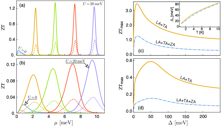
Figure 4: Left: Thermoelectric figure of merit displayed as a function of the chemical potential for temperatures (a) $T=1\,$K and (b) $T=5\,$K. Solid lines correspond for the system of Fig. 1(a), dashed lines correspond for the system of Fig. 1(b). [Remaining parameters are same as in Figs. 1(c), 1(d).] Right: Maximal value of the figure of merit for the system of Fig. 1(a), versus the energy gap for temperatures (c) $T=1\,$K and (d) $T=5\,$K. Inset in panel (c) shows the optimal gap $\Delta_{\star}$ as a function of temperature. Different lines in panels (c,d) correspond to the limit of rigid substrate eliminating ZA phonons (solid lines) or the free-standing sample (dashed-dotted lines).

Next, we investigate the figure of merit ($ZT$) given by Eq. (1). For this purpose, it is necessary to calculate both the electronic part of thermal conductance ($K_{\rm el}$), that is determined by the energy-dependent transmission $T(E)$ (see Sec. II), as well as the phononic part ($K_{\rm ph}$), presented in Fig. 3. We find that for $T<10\,$K the two systems considered show almost equal $K_{\rm ph}$ ($\propto{}T^{3}$), and different values of $ZT$ (see Figs. 4(a) and 4(b)) follow predominantly from the $G$ reduction discussed above. Unlike $|S|_{\rm max}$, a value of which (for a given $T$) is limited only by the largest experimentally-accessible $\Delta\approx{}300\,$meV Mac13 ; Zha09 , $ZT_{\rm max}$ shows well-defined conditional maximum for the optimal bandgap $\Delta_{\star}/k_{B}{}T\approx{}100-150$ (at the temperature range $10\,$K$\,\geqslant{}T\geqslant{}1\,$K) and decreases for $\Delta>\Delta_{\star}$; see Figs. 4(c) and 4(d).

Also in Figs. 4(c) and 4(d), we compare $ZT_{\rm max}$ for free-standing BLG, in which all polarizations of phonons (LA, TA, and ZA) contribute to the thermal conductance (see Supplementary Information, Sec. IV) with an idealized case of BLG on a rigid substrate, eliminating out-of-plane ($ZA$) phonons. In the latter case, $ZT_{\rm max}$ is amplified, approximately by a factor of $3$ (for any $\Delta$), exceeding $ZT=3$ for $T=1\,$K and $\Delta\approx{}\Delta_{\star}=10\,$meV.

IV Discussion

Let us now discuss here why we have identified apparently different behaviors of $|S|_{\rm max}$ and $ZT_{\rm max}$ with increasing $\Delta$. To understand these observations, we refer to the model $T^{(\alpha)}(E)$ given by Eq. (13) with $\alpha\geqslant{}0$, for which $|S|_{\rm max}^{(\alpha)}$, approximated by Eq. (III), corresponds to

$$\frac{\mu_{\rm max}^{|S|}}{k_{B}{T}} \approx{}\ln\left(\sqrt{u+\alpha}+\sqrt{u+\alpha-1}\right)$$

$$\approx{}\frac{1}{2}\ln\left(\frac{2\Delta}{k_{B}{}T}\right)\ \ \ \ \text{for }\Delta\gg{}k_{B}{}T.$$ (15)

In contrast, the chemical potential corresponding the the maximal $ZT$ is much higher and can be approximated (in the $\Delta\gg{}k_{B}{}T$ limit) by

$$\mu_{\rm max}^{ZT}\approx{}\frac{\Delta}{2}-1.145\,k_{B}{}T\ \ \ \ \text{for }\alpha=1,$$ (16)

or

$$\mu_{\rm max}^{ZT}\approx{}\frac{\Delta}{2}+0.668\,k_{B}{}T\ \ \ \ \text{for }\alpha=2,$$ (17)

where we have further supposed that $K_{\rm ph}\gg{}K_{\rm el}$, being equivalent to

$$ZT\approx{}GS^{2}\frac{T}{K_{\rm ph}(T)}.$$ (18)

As the last term in Eq. (18) depends only on $T$ we can focus now on the power factor ($GS^{2}$), a maximal value of which can be approximated by

$$\left(GS^{2}\right)_{\rm max}\approx{\cal M}_{\rm max}^{(\alpha)}\frac{g_{s}{}g_{v}{}k_{B}^{2}}{h}\left(k_{B}{}T\right)^{\alpha-1}{\cal C}(\Delta),$$ (19)

where the prefactor ${\cal M}_{\rm max}^{(\alpha)}$ depends only on $\alpha$ and is equal to $1.27$ for $\alpha=1$ or to $4.06$ for $\alpha=2$ (see also Supplementary Information, Sec. III).

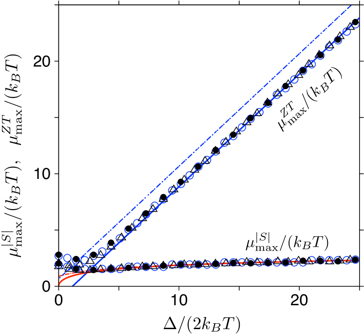
Figure 5: Chemical potential corresponding to the maximal absolute thermopower presented in Fig. 2 ($\mu_{\rm max}^{|S|}$) and the maximal figure of merit presented in Fig. 4 ($\mu_{\rm max}^{ZT}$) as function of the energy gap. Points correspond to same datasets as in Figs. 2(a) and 2(b) (skew-interlayer hopping integral is $t^{\prime}=0.3\,$eV). Lines depict approximating Eq. (IV) with $\alpha=1$ (red solid line) and $\alpha=2$ (red dash-dot line), Eqs. (16) (blue solid line), and (17) (blue dash-dot line).

The positions of maxima visible in Figs. 4(a) and 4(b) are numerically close to the approximation given by Eq. (16). Also, the data visualized in Fig. 5, together with the lines corresponding to Eqs. (16) and (17), further support our conjucture that the model $T^{(\alpha)}(E)$, given by Eq. (13) with $\alpha=1$ (the step-function model), is capable of reproducing basic themoelectric characteristics of gapped BLG with a reasonable accuracy.

Although it might seem surprising at first glance that the step-function model ($\alpha=1$) reproduces the actual numerical results much better than $T^{(\alpha)}(E)$ with $\alpha=2$, as the conductance spectra in Fig. 1(e) exhibit linear, rather than step-line, energy dependence for $\mu\geqslant{}\Delta/2$. However, for the temperature range of $1\,$K$\leqslant{}T\leqslant{}10\,$K the $T(E)$ behavior for $E-\Delta/2\gg{}0.1\,$eV, visualized with the data in Fig. 1(c), preveils [notice that the full width at half maximum for $-\partial{}f_{\rm FD}/\partial{}E$ in Eq. (II) is $\approx{}\!3.53\,k_{B}{}T\,$]. For this reason, a simple step-function model grasps the essential features of the actual $T(E)$.

Apart from pointing out that $\mu_{\rm max}^{|S|}\ll{}\mu_{\rm max}^{ZT}\approx{}\Delta/2$ for $\Delta\gg{}k_{B}{}T$ (some further implications of this fact are discussed below), the analysis starting from $T^{(\alpha)}(E)$ models also leads to the conclusion that — unlike $|S|_{\rm max}$ that is not directly related to ${\cal C}(\Delta)$ — for the figure of merit we have: $ZT_{\rm max}\propto{}(GS^{2})_{\rm max}\propto{}{\cal C}(\Delta)$ [see Eqs. (18) and (19)]. It becomes clear now that a striking $ZT_{\rm max}$ suppression for large $\Delta$ is directly link to the local $G$ suppression for large $U$, illustrated in Fig. 1(e). Power-law fits to the datasets presented in Figs. 4(c) and 4(d), of the form $ZT_{\rm max}\propto{}\Delta^{-\gamma}$ for $\Delta>\Delta_{\star}$, lead to $\gamma\approx{}0.5$. It is worth to stress here that the dispersion relation, and also the number of open channels as a function of energy above the band boundary, $N_{\rm open}(|E|-\Delta/2)$ (see Supplementary Information, Sec. II), is virtually unaffected by the increasing $\Delta$. Therefore, the average transmission for an open channel near the band boundary decreases with $\Delta$. This observation can be qualitatively understood by pointing out a peculiar (Mexican hat-like) shape of the dispersion relation for $\Delta>0$ Mac06 . In the energy range $\Delta/2<|E|<|U|/2$ there is a continuous crossover from zero transmission (occuring for $|E|<\Delta/2$) to a high-transmission range ($|E|>|U|/2$). As the width of such a crossover energy range, $(|U|-\Delta)/2$, increases monotonically with $\Delta$, the continuity of $T(E)$ implies that the average transmission near $|E|\approx{}\Delta/2$ decreases with $\Delta$.

For a bit more formal explanation, we need to refer the total transmission probability through an abrupt interface (see Supplementary Information, Sec. II). For the incident wavefunction with the momentum parallel to the barier (conserved during the scattering) $\hbar{}k_{y}$ (where $k_{y}=2\pi{}q/W$ and $q=0,\pm{}1,\pm{}2,\dots$ assuming the periodic boundary conditions) we have

$$T_{k_{y}}=\sum_{m,n}\left|t_{n}^{m}\right|^{2}j_{x}\left(\psi_{II}^{n}\right)/j_{x}\left(\psi_{I}^{m}\right),$$ (20)

where $\left\{t_{n}^{m}\right\}$ is the $2\times{}2$ transmission matrix ($m,n=1,2$ are the subband indices) to be determined via the mode-matching, and $j_{x}(\psi_{X}^{n})$ is the $x$-component of electric current for the wave function propagating in the direction of incidence, with $X=I,II$ indicating the side of a barrier. For $E=\epsilon{}+\Delta/2$ (with $0<\epsilon\ll{}\Delta/2$) there are propagating modes in a weakly-doped area ($X=II$) with $n=1$ (the lower subband) only; in the simplest case without trigonal warping ($t^{\prime}=0$) we find that the relevant current occuring in Eq. (20) scales as

$$j_{x}\left(\psi_{II}^{1}\right)\propto\sqrt{\epsilon/\Delta}.$$ (21)

The above allows us to expect that the full transmission scales as $T(E)=\sum_{k_{y}}T_{k_{y}}\propto{}\sqrt{\epsilon/\Delta}$ also for $t^{\prime}\neq{}0$, provided that the band gap is sufficiently large ($\Delta\gg{}E_{L}$, with $E_{L}=\frac{1}{4}t_{\perp}\left(t^{\prime}/t_{0}\right)^{2}$ the Lifshitz energy). As the number of propagating modes is approximately $\Delta$–independent, scaling roughly as $N_{\rm open}\propto{}\sqrt{\epsilon}$, we can further predict that zero- (or low-) temperature conductance should follow the approximate scaling law

$$G(\mu)\propto{}\left(\mu-\Delta/2\right)/\sqrt{\Delta}\ \ \ \ (\text{for }\mu\geqslant{}\Delta/2).$$ (22)

This expectation is further supported with the numerical data presented in Fig. 1(e).

An initial increase of $ZT_{\rm max}$ with $\Delta$ for $0<\Delta\ll{}\Delta_{\star}$, also apparent in Figs. 4(c) and 4(d), can be understood by pointing out that the electronic and phononic parts of the thermal conductance are of the same order of magnitude ($K_{\rm el}\sim{}K_{\rm ph}$) in such a range. In consequence, an upper bound to $ZT$ can be written as (up to the order of magnitude) $ZT\lesssim{}TGS^{2}/K_{\rm el}$, allowing a rapid increase of $ZT$ with $\Delta$ (see Supplementary Information, Sec. III), until $K_{\rm el}$ (decreasing with $\Delta$) is overruled by $K_{\rm ph}$ ($\Delta$-independent).

In the remaining part of this section, we briefly discuss the possible influence of electron-electron interactions, neglected in our numerical analysis.

Several experimental works on free-standing BLG report an intrinsic (or spontaneous) band gap of $\Delta_{\rm int}(T\!=\!0)\approx{}1.5\,$meV vanishing above the critical temperature $T_{\rm crit}\approx{}12\,$K Yan14 ; Gru15 ; Nam16 . To the contrary, no signatures of an intrinsic band gap are reported for BLG in van der Waals heterostructures (VDWHs) Kra18 , in which thermoelectric properties may be significantly enhanced due to the suppression of out-of-plane (ZA) vibrations. Possibly, the above-mentioned difference could be attributed to a modification of the effective dielectric constant due to the materials surrounding a BLG sample in VDWHs. In fact, a basic mean-field description, relating $\Delta_{\rm int}>0$ to the alternating spin order, allows one to expect that $\Delta_{\rm int}\sim{}t_{0}\exp(-{\rm const.}\times{}t_{0}/U_{\rm eff})$ (where const. $\sim{}1$ is determined by the bandwith), and thus a moderate decrease of the effective Hubbard repulsion ($U_{\rm eff}$) strongly suppresses $\Delta_{\rm int}$; see Ref. Hir85 .

Although temperatures considered in this paper ($0<T\leqslant{}10\,$K) are essentially lower then $T_{\rm crit}$, we focus on the case with a bias between the layers $|U|\approx{}\Delta\sim{}10-100\,$meV, and much smaller $\Delta_{\rm int}$ should not affect the physical properties under consideration.

Additionally, the maximal $ZT$ appears near the bottom of the conduction band or the top of the valence band ($|\mu_{\rm max}^{ZT}|\approx{}\Delta/2$), where one of the layers is close to the charge-neutrality, and thus one can expect the Coulomb-drag effects to be insignificant Gor12 .

V Concluding remarks

We have numerically investigated thermoelectric propeties of large ballistic samples of electrostatically-gapped bilayer graphene. A logarithmic deviation of the maximal absolute thermopower from the Goldsmid-Sharp relation is identified and rationalized with the help of the step-function model for the transmission-energy dependence. In addition to the earlier findings that the trigonal warping term modifies the density of states Mac13 and transport properties Sus18 also for Fermi energies $\gg{}1\,$meV, we show here that signatures of trigonal warping may still be visible in thermoelectric characteristics for the band gaps as large as $\Delta\sim{}100\,$meV.

Next, the analysis is supplemented by determining the total (i.e., electronic and phononic) thermal conductance, making it possible to calculate the dimensionless figure of merit (ZT). The behavior of maximal $ZT$ with the increasing gap can also be interpreted in terms of the step-function model, provided that we supplement the model with the scaling rule for the typical transmision probability for an open channel near the minimum of the conduction band (or the maximum of the valence band), which is $\propto{}\Delta^{-0.5}$ (for large $\Delta$). This can be attributed to the Mexican-hat like shape of the dispersion relation.

Although some other two-dimensional systems with the Mexican-hat like (or quartic) Sev17 dispersion also show enhanced thermoelectric properties, two unique features of bilayer graphene are worth to stress: (i) the possibility of tuning both the chemical potential and the band gap in a wide range, and (ii) the ballistic scaling behavior of transport characteristics with a barrier width. It is also worth to stress that the value of $ZT>1$ (or $ZT>3$ in the absence of out-of-plane vibrations) is reached at $T=1\,$K for a moderate bandgap $\Delta\approx{}10\,$meV, correponding to the electric field of $\approx{}3\,$mV/Å, making it possible to consider an experimental setup in which the spontaneous electric field from a specially-choosen substrate (e.g., ferroelectric) is employed to reduce the energy-consumption in comparison to a standard dual-gated setup Zha09 .

High values of $ZT$ at a $1\,$-Kelvin temperature may not have practical device implications per se, however, we hope that scaling mechanisms identified in our work will help to find the best thermoelectric among graphene-based (and related) systems. The necessity to reduce the phononic part of the thermal conductance with a simultaneous increase of the maximal accesible band gap (possibly in a setup not involving an extra power supply to sustain the perpendicular electric field), further accompanied by some magnification of the electric-conductance step on the band boundary, strongly suggests to focus future studies on graphene-based van der Waals heterostructures.

Author contributions

D.S. and A.R. developed the code for a rectangular BLG sample, D.S. performed the computations for a rectangular BLG sample; G.R. developed the code for the system with abrupt interface and performed the computations; all authors were involved in analyzing the numerical data and writing the manuscript.

Additional information

Supplementary information accompanies this paper.

References

- (1) Qiao, Z., Tse, W. K., Jiang, H., Yao, Y. and Niu, Q., Two-dimensional topological insulator state and topological phase transition in bilayer graphene. Phys. Rev. Lett. 107, 256801 (2011).
- (2) Maher, P. et al., Evidence for a spin phase transition at charge neutrality in bilayer graphene. Nature Phys. 9, 154 (2013).
- (3) Dean, C. T. et al., Hofstadter’s butterfly and the fractal quantum Hall effect in Moiré superlattices. Nature (London) 497, 598 (2013).
- (4) Ponomarenko, L. A. et al., Cloning of Dirac fermions in graphene superlattices. Nature (London) 497, 594 (2013).
- (5) Cao, Y. et al., Unconventional superconductivity in magic-angle graphene superlattices. Nature (London) 556, 43 (2018).
- (6) Cao, Y. et al., Correlated insulator behaviour at half-filling in magic-angle graphene superlattices. Nature (London) 556, 80 (2018).
- (7) Yang, L., Deslippe, J., Park, C. H., Cohen, M. L. and Louie, S. G. Excitonic effects on the optical response of graphene and bilayer graphene. Phys. Rev. Lett. 103, 186802 (2009).
- (8) Bonaccorso, F., Sun, Z., Hasan, T., and Ferrari, A. C., Graphene photonics and optoelectronics, Nature Photon. 4, 611 (2010).
- (9) Grigorenko, A. N., Polini, M. and Novoselov, K. S. Graphene plasmonics. Nature Photon. 6, 749 (2012).
- (10) Wang, C. R. et al., Enhanced thermoelectric power in dual-gated bilayer graphene. Phys. Rev. Lett. 107, 186602 (2011).
- (11) Chien, Y. Y., Yuan, H., Wang, C. R. and Lee, W. L., Thermoelectric Power in Bilayer Graphene Device with Ionic Liquid Gating, Sci. Rep. 6, 20402 (2016).
- (12) Mahapatra, P. S., Sarkar, K., Krishnamurthy, H. R., Mukerjee, S. and Ghosh, A., Seebeck Coefficient of a Single van der Waals Junction in Twisted Bilayer Graphene. Nano Lett., 17, 6822 (2017).
- (13) Suszalski, D., Rut, G., and Rycerz, A., Lifshitz transition and thermoelectric properties of bilayer graphene. Phys. Rev. B 97, 125403 (2018).
- (14) Lee, M. J. et al., Thermoelectric materials by using two-dimensional materials with negative correlation between electrical and thermal conductivity. Nature Commun. 7, 12011 (2016).
- (15) Sevinçli, H., Quartic Dispersion, Strong Singularity, Magnetic Instability, and Unique Thermoelectric Properties in Two-Dimensional Hexagonal Lattices of Group-VA Elements. Nano Lett. 17, 2589 (2017).
- (16) Qin, D., Yan, P., Ding, G., Ge, X., Song, H. and Gao, G., Monolayer PdSe2: A promising two-dimensional thermoelectric material. Sci. Rep. 8, 2764 (2018).
- (17) Mahan, G. D., and Sofo, J. O., The best thermoelectric. Proc. Natl. Acad. Sci. U.S.A. 93, 7436 (1995).
- (18) Kim, H.S., Liu W., Chen, G., Chu, C.W., Ren, Z., Relationship between thermoelectric figure of merit and energy conversion efficiency. Proc. Natl. Acad. Sci. U.S.A. 112, 8205 (2015).
- (19) Ioffe, A. F., Semiconductor Thermoelements and Thermoelectric Cooling. (Infosearch, London, 1957).
- (20) Cutler, M. and Mott, N. F., Observation of Anderson localization in an electron gas. Phys. Rev. 181, 1336 (1969).
- (21) Rut, G. and Rycerz, A., Minimal conductivity and signatures of quantum criticality in ballistic graphene bilayer. Europhys. Lett. 107, 47005 (2014).
- (22) Hao, L. and Lee, T. K., Thermopower of gapped bilayer graphene. Phys. Rev. B 81, 165445 (2010).
- (23) Goldsmid, H. J. and Sharp, J. W., Estimation of the thermal band gap of a semiconductor from Seebeck measurements. J. Electron. Mater. 28, 869 (1999).
- (24) McCann, E., and Koshino, M, The electronic properties of bilayer graphene. Rep. Prog. Phys. 76, 056503 (2013).
- (25) Kuzmenko, A. B., Crassee, I., van der Marel, D., Blake, P., and Novoselov, K. S., Determination of the gate-tunable band gap and tight-binding parameters in bilayer graphene using infrared spectroscopy. Phys. Rev. B 80, 165406 (2009).
- (26) Remaining parameters of the systems studied numerically are, for an abrupt interface of Fig. 1(a): m (with ); and for a rectangular setup of Fig. 1(b): .
- (27) Landauer, R., Spatial Variation of Currents and Fields Due to Localized Scatterers in Metallic Conduction. IBM J. Res. Dev. 1, 233 (1957).
- (28) Büttiker, M., Imry, Y., Landauer, R., and Pinhas, S., Generalized many-channel conductance formula with application to small rings. Phys. Rev. B 31, 6207 (1985).
- (29) Esfarjani, K., and Zebarjadi, M., Thermoelectric properties of a nanocontact made of two-capped single-wall carbon nanotubes calculated within the tight-binding approximation. Phys. Rev. B 73, 085406 (2006).
- (30) Alofi, A., and Srivastava, G. P., Thermal conductivity of graphene and graphite. Phys. Rev. B 87, 115421 (2013).
- (31) Y. Zhang, T.-T. Tang, C. Girit, Z. Hao, M. C. Martin, A. Zettl, M. F. Crommie, Y. R. Shen, and F. Wang, Direct observation of a widely tunable bandgap in bilayer graphene. Nature 429, 820 (2009).
- (32) McCann, E., Asymmetry gap in the electronic band structure of bilayer graphene. Phys. Rev. B 74, 161403(R) (2006).
- (33) Yankowitz, M. et al., Band structure mapping of bilayer graphene via quasiparticle scattering. APL Mater. 2, 092503 (2014).
- (34) Grushina, A.L., Ki, D.-K., Koshino, M., Nicolet, A. A. L., Faugeras, C., McCann, E., Potemski, M., and Morpurgo, A. F., Insulating state in tetralayers reveals an even-odd interaction effect in multilayer graphene. Nat. Commun. 6 6419 (2015).
- (35) Nam, Y., Ki, D.-K., Koshino, M., McCann, E., and Morpurgo, A. F., Interaction-induced insulating state in thick multilayer graphene. 2D Mater. 3, 045014 (2016).
- (36) Kraft, R. et al., Tailoring supercurrent confinement in graphene bilayer weak links. Nature Commun. 9, 1722 (2018).
- (37) J. E. Hirsch, Two-dimensional Hubbard model: Numerical simulation study. Phys. Rev. B 31, 4403 (1985).
- (38) Gorbachev, R. V., Geim, A. K., Katsnelson, M. I., Novoselov, K. S., Tudorovskiy, T., Grigorieva, I. V., MacDonald, A. H., Morozov, S. V., Watanabe, K. , Taniguchi, T., and Ponomarenko, L. A., Strong Coulomb drag and broken symmetry in double-layer graphene. Nature Phys. 8, 896 (2012).