Concept-drifting Data Streams are Time Series;
The Case for Continuous Adaptation

Abstract

Learning from data streams is an increasingly important topic in data mining, machine learning, and artificial intelligence in general. A major focus in the data stream literature is on designing methods that can deal with concept drift, a challenge where the generating distribution changes over time. A general assumption in most of this literature is that instances are independently distributed in the stream. In this work we show that, in the context of concept drift, this assumption is contradictory, and that the presence of concept drift necessarily implies temporal dependence; and thus some form of time series. This has important implications on model design and deployment. We explore and highlight the these implications, and show that Hoeffding-tree based ensembles, which are very popular for learning in streams, are not naturally suited to learning within drift; and can perform in this scenario only at significant computational cost of destructive adaptation. On the other hand, we develop and parameterize gradient-descent methods and demonstrate how they can perform continuous adaptation with no explicit drift-detection mechanism, offering major advantages in terms of accuracy and efficiency. As a consequence of our theoretical discussion and empirical observations, we outline a number of recommendations for deploying methods in concept-drifting streams.

1 Introduction

Predictive modeling for data streams is becoming an increasingly-relevant task, in particular with the increasing advent of sensor networks and tasks in artificial intelligence, including robotics, reinforcement learning, system monitoring, anomaly detection, social network and media analysis.

In a data stream, we assume that data arrives

$$(\mathbf{x}_{t},y_{t})\sim p_{t}(\mathcal{X},\mathcal{Y})$$

over time $t=1,\ldots,\infty$. A model observes test instance $\mathbf{x}_{t}$ and is required to make a prediction

$$\hat{y}_{t}=h_{t}(\mathbf{x}_{t})$$

at time $t$. Hence the amount of computational time spent per instance must be less that the rate of arrival of new instances (i.e., the real clock time between time steps $t-1$ and $t$). A usual assumption is that true label $y_{t-1}$ becomes available at time $t$, thus allowing to update the model.

This is in contrast to a standard batch setting, where a dataset $\{\mathbf{x}_{t},y_{t}\}_{t=1}^{N}$ of fixed $N$ is observed prior to inducing the model. See [11] for introduction and definitions.

1.1 Building Predictive Models from Data Streams

We wish to build a model that approximates, either directly or indirectly, the generating distribution. For example, a MAP estimate for classification

$$\hat{y}_{t}=h_{t}(\mathbf{x}_{t})=\operatornamewithlimits{argmax}_{y}\tilde{p}_{t}(\mathbf{x}_{t},y)$$

The incremental nature of data streams has encouraged a focus on fast and incremental, i.e., updateable, models; both in the classification and regression contexts. Incremental decision trees such as the Hoeffding tree (HT, [15]) have had a huge impact on the data-streams literature and dominate recent output in this area. They are fast, incremental, easy to deploy, and offer powerful non-linear decision boundaries. Dozens of modifications have been made, including ensembles [6, 18, 13, 12], and adaptive trees [4].

High performance in data streams has also been obtained by $k$-nearest neighbors ($k$NN) methods, e.g., [19, 26, 25]. As a lazy method, there is no training time requirement other than simply storing examples to which – as a distance-based approach – it compares current instances, in order to make a prediction. The buffer of examples should be large enough to represent the current concept adequately, but not too large as to be prohibitively expensive to query.

Methods employing stochastic gradient descent (SGD) have been surprisingly underutilized in this area of the literature. Baseline linear approaches obtained relatively poor results, but can be competitive with appropriate non-linearities [20] and have been used within other methods, e.g., at the leaves of a tree [1]. In this work, we argue that the effectiveness of SGD methods on data-stream learning has been underappreciated and in fact offer great potential for future work in streams.

1.2 Dealing with Concept Drift

Dealing with concept drift, where the generating distribution $p_{t-1}\neq p_{t}$ in at least some part of the stream, is a major focus of the data-stream literature, since it means that the model current $h_{t}$ has become partially or fully invalid. Almost all papers on the topic propose some way to tackle its implications, e.g., [14, 28, 11, 6, 18, 16, 17]. A comprehensive survey to concept drift in streams is given in [11].

The limited-sized buffer of $k$NN methods imply a natural forgetting mechanism where old examples are purged, as dictated by available computational (memory and CPU) resources. Any impact by concept drift is inherently temporary in these contexts. Of course, adaptation can be increased by flushing the buffer when drift is detected.

HTs can efficiently and incrementally build up a model over an immense number of instances without needing to prune or purge from a batch. However, a permanent change in concept (generating distribution) will permanently invalidate the current tree (or at least weaken the relevance of it – depending on severity of drift) therefore dealing with drift becomes essential. The usual approach is to deploy a mechanism to detect the change, and reset a tree or part of a tree when this happens, so that more relevant parts may be grown on the new concept. Common detection mechanisms include ADWIN [3], CUMSUM [22], Page Hinkley [7], and various geometric moving average and statistical tests [10]. For example, the Hoeffding Adaptive Tree (HAT, [4]) uses an off-the-shelf ADWIN detector at each node of a tree, and cuts a branch at a node where changes in registered. It is expected that the branch will be regrown on new data and thus represent the new concept. Tree approaches are almost universally employed in ensembles to mitigate potential fallout from mis-detections.

In this paper we argue strongly for the potential importance of a third option – of continuous adaptation, where knowledge (e.g., a set of parameters determining a decision boundary) is transferred as best as possible to a newer/updated concept rather than discarded or reset as in currently the case with the popular detect and reset approach. This possibility can be enacted with SGD. SGD is intimately known and widely used across swathes of the machine learning literature, however, we note that it is markedly absent from the bulk of the data-stream methods, and often only compared to only as a baseline in experiments. In this paper we argue that it has been discarded prematurely and underappreciated. We analyse and parameterize it specifically in reflection to performance in concept-drifting data-streams, and show it to be very competitive with other approaches in the literature (results in Section 7).

To summarize the main mechanisms to deal with concept drift:

1. Forgetting mechanism
   (e.g., $k$NN, and batch-incremental ensembles)

2. Detect and reset mechanisms
   (e.g., HATs and HT-ensembles with ADWIN)

3. Continuous adaptation
   (e.g., SGD-based models incl. neural networks)

1.3 Organization and contributions

In spite of the enormous popularity of ensembled trees and distance-based ($k$NN) approaches, we will show that continuous adaptation can be more suited to concept-drifting data streams. We do this by breaking with a common assumption.

Namely, existing work in data streams is mostly based on the assumption of i.i.d. data within a particular concept; therefore seeking as an objective to detect a change in concept, so that off-the-shelf i.i.d. models can be (re)-deployed. A model belonging to a previous concept is seen as invalid. This leads to the detect-and-reset approach to dealing with concept drift mentioned above. In this work, on the contrary, we show that drift inherently implies temporal dependence; that all concept-drifting streams are in some way a time series, and can be treated as such. We propose to treat the concept as a temporal sequence, to enable continuous adaptation as an effective alternative to detect-and-reset approaches. For this purpose we derive gradient descent approaches; and we show scenarios where they compare very favorably in comparison with more popular tree and distance-based methods. The contributions of this work can be summarized as follows:

• We show that concept-drifting data streams can be considered as time series problems (Section 2)

• Following a fresh analysis on concept drift (Section 3), we conduct a bias-variance analysis of learning under drift, and derive gradient descent approaches for concept-drifting data streams in the framework of continuous adaptation (Section 4)

• We give an analytical and empirical investigation (Section 6) which highlights properties of our suggested approach; and from the results (displayed and discussed in Section 7) we outline the implications and make a number of recommendations before making concluding remarks (Section 8).

2 Concept-drifting Streams are Time Series

Concept-drifting data streams have been widely treated under the assumption of independent samples (see, e.g., [10, 6, 11, 27] and references therein). In this section, we argue that if a data stream involves concept drift, then the independence assumption is violated.

If data points are drawn independently, we should be able to write

$$p_{t}(y_{t},x_{t},x_{t-1}) =p_{t}(y_{t}|x_{t})p_{t}(x_{t-1})$$ (1)

$$p_{t}(y_{t}|x_{t},x_{t-1}) =p_{t}(y_{t}|x_{t})$$

see Figure 1a for illustration, where the lack of an edge between time-steps indicates the independence.

The subscript of $p_{t}$ reminds us of the possibility of concept drift (in which case, $p_{t}\neq p_{t-1}$).

Lemma 1.

A data stream that exhibits a concept drift also exhibits temporal dependence.

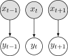
(a)

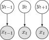
(b)

Figure 1: The ‘standard’ discriminative LABEL:sub@fig:main_figure.a and generative LABEL:sub@fig:main_figure.a_bis models for prediction in data streams; as directed probabilistic graphical models.

Proof.

Let $p_{t}(y_{t}|x_{t})=p(y_{t}|x_{t},C_{t})$ where $C_{t}\in\{0,1\}$ denotes the concept at time-step $t$, and let the drift occur at point $0<\tau<\infty$. Thus $C_{t}=0$ for $t<\tau$, and $C_{t}=1$ for $t\geq\tau$. Under independence,

$$P(C_{t})=P(C_{t}|C_{t-1})$$

However, it is obvious that

$$P(C_{t}=0)\neq P(C_{t}=0|C_{t-1}=1),$$

namely, after the drift we no longer expect instances from the first concept.

We can use the joint distribution, Eq. (1), to check for independence, for any particular time step $t$, marginalizing out $C$ which is not observed:

$$p(y_{t}|x_{t},x_{t-1}) \propto p(y_{t},x_{t},x_{t-1})$$

$$=\sum_{c_{t},c_{t-1}}p(y_{t},x_{t},c_{t},c_{t-1},x_{t-1})$$

$$=p(y_{t}|x_{t})\underbrace{\sum_{j=1}^{t}\sum_{c_{j},c_{j-1}}p(x_{j}|c_{j})p(c_{j}|c_{j-1})}_{p(x_{t}|x_{t-1})}$$

$$=p(y_{t}|x_{t})p(x_{t}|x_{t-1})$$ (2)

which does not equal Eq. (1), thereby indicating temporal dependence (via the presence of $t-1$). ∎

This can be visualized as a probabilistic graphical model in Figure 2a (observed variables are shaded); and in Figure 2b with concept drift marginalized out.

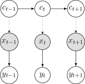
(a)

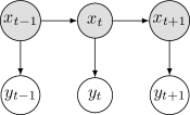
(b)

Figure 2: A discriminative model LABEL:sub@fig:main_figure.b for prediction in data streams with concept drift (dashed lines simply indicate that these connections are not usually explicitly addressed). When drift is taken into account and marginalized out LABEL:sub@fig:main_figure.c, inputs become connected.

We have shown above that data streams with concept drift exhibit temporal dependence, which essentially means that all such streams can be seen as a time series.

We have done this analysis in the most extreme case of a switch in concepts over a single time step (a sudden change in concept). One might argue that as $t\rightarrow\infty$, the importance of the dependence resulting from this one-time drift becomes negligible, since after drift, $P(C_{t}=1)=P(C_{t-1})=1$ and could thus be considered a constant essentially rendering independence within each concept. However we do not observe $\tau$; we cannot know exactly when the drift will occur or if it has ocurred. As a result, an instantaneous drift between two time steps can manifest itself as temporal dependence in the error signal over many instances. It is surprising that this is not explicit across the literature, since it is indeed implicit in most change-detection algorithms, in the sense that they measure the change in the error signal of predictive models.

The relationship between the predictive model and the error is clearly seen in the relation

$$E_{t}=E(h_{t}(\mathbf{x}_{t}),y_{t})$$

where $E$ is the error function (e.g., mean-squared or classification error, depending on the problem). Clearly if $h_{t}$ is poorly adapted to deal with a concept drift, this will appear in increasing $E_{t}$ (i.e., a time series). It is illustrated (for incremental drift) in Figure 3. Rather than monitoring $\{E_{t}\}$ for drift so as to reset $h_{t}$, in this paper, we look at adapting $h_{t}$ directly.

Having argued that concept drifting streams are time series – should we just apply off-the-shelf time series models? Expanding on some differences mentioned in [27], we can point out that

1. Only data streams exhibiting concept drift are guaranteed to have time series elements, and only in consideration specifically of these parts of the stream

2. Time dependence in data streams it is seen as a problem (something to deal with), rather than as part of the solution (something to explicitly model)

3. In data streams the final estimation of each $\hat{y}_{t}$ is required at time $t$, and thus retrospective/forward-backward (smoothing) inference (as is typical in state-space models) is not applicable

4. A common assumption in data streams is that the ground truth is available at time $t-1$, providing a stream of training examples $(\mathbf{x}_{t-1},y_{t-1})$ whereas time series models are typically built offline before being deployed live

5. Data streams are assumed to be of infinite length (therefore, also training data, on account of item 4)

Some of these assumptions are broken on a paper-by-paper level. For example, changes to point 4 have been addressed in, e.g., [12, 14].

The most closely related time series task to prediction in streams is that known as filtering. Actually, Eq. (2) is a starting point for state space models such as hidden Markov models, Kalman and paricle filters (see [2] for a thorough review) for which filtering is a main task, although these models are not usually expected to be updated at each timestep as in the streaming case (a possibility due to point 4 above).

Although we cannot always apply state-space models directly to data streams, we nevertheless remark again that temporal dependence plays a non-negligible role, and can be leveraged as an advantage. In particular, in reflection of this section, we next make a revision of concept drift – in Section 3 – which then allows us to employ efficient and effective methods (Section 4), allowing us to draw conclusions that have important repercussions in data streams mining.

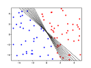
(a)

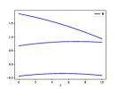
(b)

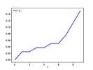
(c)

Figure 3: Concept drift (incremental drift): decision boundary on $y_{t}=\sigma(\theta_{t}^{\top}\mathbf{x}_{t})$ shown for $t=\tau,\tau+1,\ldots,\tau+10$ LABEL:sub@fig:drift_series.a; corresponding value of the coefficients over these time-steps LABEL:sub@fig:drift_series.b – forming a time series with obvious temporal dependence: $\theta_{\tau},\ldots,\theta_{\tau+10}$; and the error rate over time – also a clear time series LABEL:sub@fig:drift_series.c.

3 Types of Concept Drift: A Fresh Analysis

Sudden, complete, and immediate drift is widely considered in the literature (and for this reason we worked with it in the previous section), yet we could also argue that gradual, or incremental drift fit better a dictionary definition which implies a movement or tendency and are more widespread in practice. A complete change in concept simply means we have changed problem domains. The idea of a movement inherently includes the implication of dependence (e.g., across time and space) – and dependence (among instances) implies naturally a time series – as we have elaborated in the previous section.

Let us review and revise concept drift, based on the types of drift identified in [11], which relist for convenience:

1. Sudden/abrupt

2. Incremental

3. Gradual

additionally noting the possibility of reoccurring drift which may involve any of these types and, noting also the related task of dealing with outliers, which are not concept drift.

In the following, we denote $\theta_{t}\in\Theta$ as the true (unknown) parameters defining the current concept at time $t$, i.e., $p_{\theta_{t}}$. This allows for a smooth drift across concept space $\Theta$ (for example, a set of coefficients defining a hyperplane; see Figure 3) but also allows for a qualitative view of categorical concepts $C_{t}\in\{1,\ldots,K\}$; such that $\theta^{c}$ represents the parameters of the $c$-th concept; i.e., we would speak of drift between concepts $\theta^{{1}}$ and $\theta^{{2}}$.

3.1 Abrupt change

If the concept changes abruptly, in either a partial or complete manner, we may denote

$$\theta_{t}=\begin{cases}\theta^{c_{1}}&t<\tau\\ \theta^{c_{2}}&t\geq\tau\end{cases}$$ (3)

for some time index $\tau$ where the ‘drift’ occurs. The drift may be total ($\theta^{1}$ and $\theta^{2}$ are drawn independently from $\Theta$) or partial (only a local change, to some part of $\theta$.

3.2 Incremental drift

Incremental drift denotes a change over time. It can be denoted as an additive operation, where the current concept can be written as

$$\theta_{t}=\theta_{t-1}+\Delta_{t}\theta$$ (4)

i.e., an increment of $\Delta_{t}\theta$. We generally assume that drift is active in range $\tau_{1}\leq t\leq\tau_{2}$ (and that $\Delta\theta=0$ outside of this range); where concept $c_{1}$ before, $c_{2}$ after, and a blended mixture inbetween).

3.3 Gradual drift

In gradual drift, drift also occurs over time, but in a stochastic way. We may write

$$\theta_{t}=\theta^{c_{t}}\quad\text{ where }\quad{c_{t}}\sim\mathcal{B}(\alpha_{t})$$ (5)

where $c_{t}=1$ with probability $\alpha_{t}$, and $c_{t}=2$ otherwise; $\mathcal{B}$ being a Bernoulli distribution. Note that $\alpha_{t}$ is itself is an incremental drift (see Eq. (4)) between values $0$ and $1$. The stream thus increasingly-often generates examples from the new concept $c_{2}$; where drift $\alpha_{t<\tau_{1}}=0$ and $\alpha_{t>\tau_{2}}=1$ outside of the drift range $\tau_{1},\ldots,\tau_{2}$.

Note that neither incremental nor gradual drift need be smooth or monotonically increasing, although that is a common simplification. A sigmoid function is often used in the literature; as in many of the stream generators of the MOA framework [5].

3.4 Re-occurring drift

Re-occurring drift may be any of the above cases (sudden, gradual, or incremental) where a concept may repeat at different parts of the stream. It is very much related to the idea of state-space models such as hidden Markov models, and switching models (both are reviewed in [2]). We remark that there is no technical difference between modelling states, and tracking concepts. Usually we can distinguish a state as something that we want to model (e.g., a weather system), and a concept drift as something we wish to adapt to or take into account (e.g., change/degradation of in the monitoring sensors, or climate change).

4 Learning under Drift: Theoretical Insights

In this section we investigate an approach to adapt to drift continuously as part of the learning process, rather than reactively (i.e., the detect-and-reset approach) using explicit drift detection mechanisms, as has previously been the main approach (see Section 1).

It is well known that prediction error of supervised learners breaks down into variance, bias, and irreducible error (see, e.g., [2, 9]). Let $f:\mathcal{X}\rightarrow\mathbb{R}$ represent the true underlying (unknown) model parametrized by $\theta_{c}$, which produces observations $y_{t}=f(\mathbf{x}_{t};\theta_{c})+\epsilon_{t}$, where $\epsilon_{t}\sim\mathcal{N}(0,\sigma^{2})$. The expected mean squared error (MSE) over the data, with some estimated model $h$, can be expressed as

$$\mathbb{E}_{\mathbf{x}_{t}}[\textsf{MSE}(h,y|\mathbf{x}_{t})] =\mathbb{E}_{\mathbf{x}_{t}}\mathbb{E}_{y_{t},\epsilon_{t}}[(y_{t}-h)^{2}|\mathbf{x}_{t}]$$

$$=\sigma^{2}+\mathbb{V}[h]+\mathbb{E}[f-h]^{2}$$ (6)

i.e., irreducible noise, variance, and bias² terms, respectively.

The result in Eq. (6) hinges on the assumption that $\mathbb{E}[y]=\mathbb{E}[f+\epsilon]=f$ due to the fact that $\mathbb{E}[\epsilon_{t}]=0$.

However, recall that in the case of concept drifting data streams, $f$ is not constant, but inherits randomness from random variable $C_{t}$ (see Sections 2 and 3). We can get around this problem by taking the expectation of MSE within each concept; wrt the point of a single change (which we denote $\tau$), then for time $t\geq\tau$),

$$y_{t}=\underbrace{\left[f_{t<\tau}+\Delta(f_{t<\tau},f_{t\geq\tau})\right]}_{f_{t\geq\tau}}(\mathbf{x}_{t})+\epsilon_{t}$$

where $\Delta(f_{t<\tau},f_{t\geq\tau})$ represents the change in concept. Regarding Eq. (6): At $t=\tau$ the third term (bias) is now essentially the difference between the current true concept, and an estimated old concept. In other words (in terms of parameters),

$$(\theta_{t}-\hat{\theta}_{t})^{2}$$ (7)

and clearly the obvious goal (in terms of reducing bias), is moving $\hat{\theta}_{t}$ (an estimate of the previous concept) towards $\theta_{2}$ (the true current concept), and over a concept drifting stream of multiple drifts of different types: to model the journey of $\theta$.

In the data streams literature, ensemble models with drift-detection strategies have blossomed (see, [13, 18] for surveys). We can now describe theoretical insights to this popularity in this particular area: By resetting a model when drift is detected, it is possible to reduce the bias implied by the drift in those models. However, this may increase the variance component of the error (since variance can be higher on smaller datasets [8]). Ensembles are precisely renown for reducing the variance component of the error (see., e.g., [9] and references therein) and thus desirable to counteract it.

This analysis also leads us once more to the downside of this approach: Under long and intensive drift, a vicious circle develops; increased efforts to detect drift lead to more frequent detections and thus frequent resetting of models (implicitly, to reduce bias), which encourages the deployment of ever-larger ensembles (to reduce the variance caused precisely by resetting models). As seen in the literature, ensemble sizes continue to grow; and our experiment section confirm that such implementations can require significant computational time.

Methods with an explicit forgetting mechanism (e.g., $k$NN, batch-incremental methods – also popular in the literature) will automatically establish ‘normal’ bias as $(t-\tau)$ becomes as large as the maximum number of instances stored in memory. However, this can be a long time if that size is large; and not a solution when the drift is sustained over a long time or occurs regularly.

Finally, we remark again that detectors will fire when the error signal has already shown a significant change, by which time many (possibly very biased) predictions may have been made.

In the following section we discuss how to avoid this trade-off. Namely, we propose strategies of continuous adaptation which do not detect drift, but track drift through time.

5 Continuous Adaptation under Concept Drift

Drift detection methods usually monitor the error signal retrospectively for change (is $\epsilon_{t}$ statistically different from $\epsilon_{t-1},\epsilon_{t-2},\ldots$; a warning can be raised). However, since – as argued above – concept drift can be seen as a time series we can attempt to forecast and track the drift, and adapt continuously.

In this sense, solving the concept drift problem is identical to solving the forecasting problem of predicting $\theta_{t}$ which defines the true unknown concept (see Eq. (7)). Using all the stream we have seen up to timestep $t$, we could write

$$\hat{\theta}_{t}=g(\mathbf{x}_{1},\ldots,\mathbf{x}_{t},y_{1},\ldots,y_{t-1})$$

which at first glance appears unusable because it is a function over an increasingly large window of data. However, using a recursion on $\hat{\theta}_{t-1}$, for minimizing least mean squares, there is a closed-form solution: recursive least squares (RLS), which uses recursion to approximate

$$\hat{\theta}_{t}=\hat{\theta}_{t-1}+\mathbf{R}^{-1}_{t}\mathbf{x}_{t}(y_{t}-\mathbf{x}_{t}^{\top}\hat{\theta}_{t-1})$$

where $\mathbf{R}^{-1}_{t}=\mathbf{R}^{-1}_{t-1}-\mathbf{R}^{-1}_{t-1}\mathbf{x}_{t}(1+\mathbf{x}_{t}^{\top}\mathbf{R}^{-1}_{t-1}\mathbf{x}_{t})^{-1}\mathbf{x}^{\top}_{t}\mathbf{R}^{-1}_{t-1}$.

RLS is a well known adaptive filter, which can be easily extended to forgetting-RLS and Kalman filters (see, e.g., [9]).

Noting that $\mathbf{x}_{t}(y_{t}-\mathbf{x}_{t}^{\top}\hat{\theta}_{t-1})=\nabla E_{\hat{\theta}_{t}}$ and replacing $\mathbf{R}^{-1}_{t}$ with learning rate $\lambda$ we derive stochastic gradient descent (SGD), as follows.

For $t=1,\ldots,\infty$:

$$\hat{y}_{t} =h(x_{t};\hat{\theta}_{t})$$

$$\Delta\hat{\theta}_{t} =\lambda\nabla E_{\hat{\theta}_{t}}(\hat{y}_{t},y_{t})$$

$$\hat{\theta}_{t+1} \leftarrow\hat{\theta}_{t}+\lambda\nabla E_{\hat{\theta}}=\hat{\theta}_{t}+\Delta\hat{\theta}_{t}$$

where the last line is essentially forecasting the concept for the following timestep (note the connection to, e.g., Eq. (4)). Note the data-stream assumption that at time-point $t+1$ we have already observed the true value $y_{t}$.

This may be viewed as a trivial result, but it has important implications regarding much of the data-stream research and practice, which traditionally relies predominantly on ensembles of decision trees or $k$-nearest neighbor-based methods; see Section 1.1. We have argued that it has been underappreciated. Unlike Hoeffding tree methods, a gradient-descent based approach can learn from a concept-drifting stream without explicit concept drift detection. Unlike $k$NN, time complexity is much more favourable.

We remark that for SGD to perform robustly over the length of a stream, we have to ensure certain conditions. In particular, to not decay the learning rate $\lambda$ towards zero over time. In batch scenarios wish wish to converge to a fixed point and such learning rate scheduling is common and effective practice. However, under as stream this would cause SGD to react more and more slowly to concept drift until eventually becoming stuck in one concept.

An illustration of how SGD performs in a constant-drift setting is given in Figure 4 on a synthetic data stream (which is detailed later in Section 6). We clearly see how no drift detection or model reset is necessary, and a concept can be smoothly tracked in its drift through concept space.

(a)

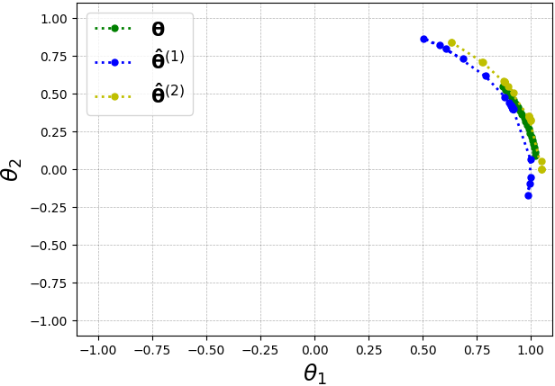
(b)

(c)

Figure 4: Data points from a stream exhibiting concept drift LABEL:sub@f:a; where the true concept is represented as a decision boundary $\theta^{\top}\mathbf{x}=0$ (shown in green) which is rotating clockwise; and estimates $\hat{\theta}_{t}$ (in blue and yellow) are following it. Both are SGD methods with learning rate $\lambda=0.5$, and the blue has an additional momentum term $\beta=0.5$. We see the path through weight/concept space LABEL:sub@f:b, i.e., the concept drift. Rather than a reactive approach monitoring the error rate retrospectively, $\hat{\theta}_{t+1}\approx\theta_{t+1}$ can be tracked and pre-empted. Drift is constant across this time window, yet error rate $\epsilon_{t}|t=1,2,\ldots$ recedes LABEL:sub@f:c as $\hat{\theta}$ converges on the true moving concept. We emphasise that predictive performance improves during the drift.

Recall that under gradual drift, it is the $\alpha_{t}$ (see Eq. (5)) rather than $\theta_{t}$ which forms a time series. A detailed treatment is left for future work.

Since abrupt drift cannot necessarily be forecast in advanced, one might argue that traditional drift detectors are best suited to this case. We remark that this argument can be clearly accepted only under the condition of a complete change in concept; where the two tasks are not at all related; a scenario unlikely to be the case in practice. If the drift is partial (i.e., the two concepts are partially related), then we wish to transfer part of the old concept (i.e., not discard it when drift is detected). We note that SGD, in this sense, performs a kind of transfer learning; namely continuous transfer learning. The literature on transfer learning (see, e.g., [23]) indicates that we are thus likely to learn the new concept much faster.

6 Experiments

We carried out a series of experiments to enrich the discussion and support the arguments made in this work. All methods are implemented in Python and evaluated in the Scikit-MultiFlow framework [21] under prequential evaluation (testing then training with each instance). Experiments are carried out on a desktop machine, 2.60GHz, 16GB RAM.

First, we generated synthetic data using a weight matrix $\theta_{c}\sim\mathcal{N}(\mathbf{0},\mathbf{I})$ to represent the $c$-th concept. We introduced drift using the equations Eq. (3), Eq. (4), Eq. (5), under parameters in Table 1. For incremental drift,

$$\theta_{t}=A_{0.01}^{\top}\theta_{t-1}=\theta_{t-1}+\Delta_{t}\theta$$

where $A_{0.01}$ is a rotational matrix (of angle $0.01$ in radians); for gradual drift,

$$\alpha_{t}=p(c_{t}=1)=\frac{1}{\tau_{2}-\tau_{1}}(t-\tau_{1}).$$

and, for sudden drift a new $\theta_{t}\sim\Theta$ is simply re-sampled after timestep $\tau_{1}$.

Table 1: Parameters for synthetic data, except: $\tau_{2}=\tau_{1}+1$ in the case of sudden drift, and clearly $\tau_{1},\tau_{2}$ are not used at all if no drift. In all experiments, accuracy is recorded over instances $\tau_{0},\ldots,T$.

Sym.	$t$	Description
$\tau_{0}$	$T/10$	pre-training ends
$\tau_{1}$	5K	start of drift
$\tau_{2}$	6K	end of drift (gradual, incr.)
$\tau_{2}$	$\tau_{1}+1$	end of drift (sudden)
$T$	10K	length of stream

We additionally look at two common benchmark datasets from the data-streams literature involving real-world data: the Electricity and CoverType datasets. Electricity contains 45,312 instances, with has $6$ attributes describing an electricity market (the goal is to predict the demand). CoverType contains 581,012 instances of 54 attributes, as input to predict one of seven classes representing forest cover type. See, e.g., [10, 24, 4, 12] for details.

We employed the three main approaches discussed in this work (listed in Table 2); both a vanilla configuration (‘stardard’ $k$NN, SGD, HT) and an ‘advanced’ configuration of the same methodologies. For HT and $k$NN we used state-of-the-art adaptations. For SGD, we simply employed basis expansion to accommodate non-linear decision boundaries.

Table 2: Methods and their parameterization, both for a ‘standard’ implementation (Vanilla Configuration) and high-performance (Advanced Configuration). Values for any parameters not shown can be found as the default parameters in ScikitMultiflow (v0.1.0 used here).

$k$NN	$k=10$, buffer size 100
SGD	$L_{2}$ regularization; $\lambda=0.01$, hinge loss
HT	$10^{-7}$ split confidence, 0.05 tie threshold, naive Bayes at leaves
SAM$k$NN	Self-adjusting memory $k$NN [19]
PBF-SGD	SGD with deg. $3$ polynomial basis expansion, e.g., [9]
RF-HT	Adaptive Random Forest [12]: an ensemble of $100$ HTs, ADWIN drift detection, $\lambda=6$, $n_{min}=50$

First we had a look at performance on the synthetic data (Figure 5), then on real world data (Figure 7), and finally, on an especially challenging scenario (Figure 6) over a sustained incremental drift. Table 3 summarizes the predictive performance and Table 5 provides some running time results.

7 Discussion

We present and discuss results from the experiments outlined in the previous section.

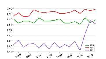
(a)

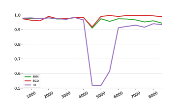
(b)

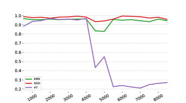
(c)

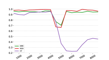
(d)

Figure 5: Results (classification accuracy over a sliding window of $200$ instances on synthetic streams. Notice that the vertical axes are scaled for greater visibility of separation.

Hoeffding Trees are fast but conservative

We observe how HTs grow conservatively (Figure 5a). This behaviour is intended by design, since they have no natural forgetting mechanism and thus it is important to make a statistically safe split (based on the Hoeffding bound).

Indeed, note after $t=7000$ accuracy jumps 10 percentage points; indicating the initial split.

This conservative approach provides strong confidence that we may produce tree equivalent to one built from a batch, but only within a single concept. It necessarily means that Hoeffding trees will struggle when the true target concept $\theta_{t}$ is a moving target rather than a fixed point in concept space.

And we observe this: Figures 5b—5d show how the performance of a standalone HT is damaged by concept drift (as opposed to SGD- and $k$NN-based methods which are able to recover more quickly.

Destructive adaptation is costly

In the literature sophisticated concept-drift detectors and ensembles are used to counteract this disadvantage, and provide robust prediction in dynamic data streams. And we confirm that this approach is effective in many cases (as seen in Figure 7) but at a significant cost: the computational time (see Table 5) of the detect-and-reset approach clearly enunciates the overhead of destroying (resetting) and regrowing HTs constantly, so as to adapt to a changing concept.

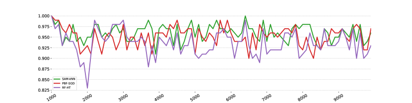
Figure 6: An incremental drift scenario like that of Figure 5 except that the drift is constant across the entire stream ($\tau_{1}=\tau_{0}$, and $\tau_{2}=T$ wrt Table 1).

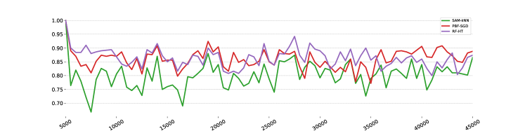
(a)

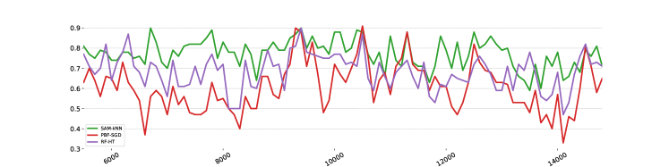
(b)

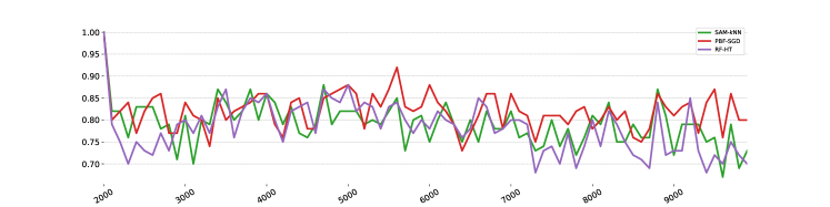
(c)

Figure 7: Average accuracy over sliding window of 200 for methods detailed in column 3 of Table 2. For visualization, we plot only a subset of CoverType. See Table 3 for total accuracy over the streams.

Buffer-based methods are limited

Respective of its buffer size, $k$NN-methods can respond to drift by forgetting old instances (from old concepts) and taking in (i.e., learning from) new ones. This mechanism allows it to recover quickly from drift (Figure 5b–Figure 5d). Nevertheless predictive power is always limited in proportion to the number of instances stored in this buffer and, as observable in Figure LABEL:sub@f:synth.a, sometimes this is insufficient (we note there is no upward trend here, as opposed to the other methods, despite more instances from the same concept). If buffer size is widened, performance can be higher, but adaptation to drift will take correspondingly longer or require explicit drift detection methods as with HT approaches.

SGD for Efficient Continuous Adaptation

SGD is a simple method which has been around a long time. With a non-decayed learning rate, we find that it behaves as well as we hypothesized on synthetic data: it continues to learn a static concept better over time (in Figure 5a it recovers quickly from sudden and gradual drift, and its performance is almost unaffected under incremental drift where (as we see in Figure 5c) it is able to adapt continuously.

We suspect that SGD has not been widely considered in state-of-the-art data-stream evaluations because it performs poorly on real-world and complex data when deployed in an off-the-shelf manner, especially if the learning rate is decayed – as is often the standard. However, we put together the PBF-SGD method from elementary components and find that it performs strongly in these scenarios (Figure 6, Figure 7).

We do see that performance of the advanced/state-of-the-art methods (HT and $k$-NN based) is also competitive, as expected, yet it is crucial to emphasise the difference in computational performance (see Table 5): running time is up to an order of magnitude or more higher for the decision tree ensemble, compared to other methods; even greater than PBF-SGD, which has a feature space cubicly greater than the original.

An analysis of time and memory complexity

The worst-case complexity is outlined in Table 4 (for the vanilla methods, which does not take into account the additional overhead of ensembles and drift detectors nor basis expansion for PBF-SGD). We can further remark computational time and memory expectations of SGD are constant across time (the expected running time is the same for each instance in the stream), as also with $k$NN (given a fixed batch size). On the other hand, HT costs are not constant, but continue to grow with the depth of the tree (the $\ell$ term in Table 4). This is an issue which as, to our knowledge, not been considered in depth in the literature: as trees in an ensemble grow and are reset under drift, time and space complexity fluctuates – making practical requirements difficult to estimate precisely in advance. If there is no drift – then the trees may, in theory, grow unbounded and use up all available memory.

Table 3: Overall accuracy (average over entire stream) of methods; seen also in experiments of Figure 6 (regarding the Synthetic stream) and Figure 7 for the others.

	SAM$k$NN	PBF-SGD	RF-HT
Electricity	79.8	85.9	86.2
RTG	78.8	81.8	77.9
CoverType	93.3	92.6	93.9
Synthetic	96.0	95.1	93.6

Table 4: An outline of time and space complexity for different methods, with a moving window of $w$ examples, taking the $k$ nearest neighbors (for $k$NN), in a problem of $d$ attributes. For HT, $\ell$ is the number of leaves, but note that this is $O(n)$ in the worst case. To simplify, we have considered a binary ($2$ class) problem with one split considered per attribute in the case of trees.

Method	Time	Space
$k$NN	$O(wdk)$	$O(wd)$
HT	$O(d)$	$O(\ell d)$
SGD	$O(d)$	$O(d)$

Table 5: Total running time under prequential evaluation (in seconds) on a selection of the datasets. We compare SGD with both polynomial of degree 2 and 3 (PBF-SGD(2) and (3), respectively) – for sake of comparison. Synth refers to the data of Figure 6. The time including the initial block (which is not evaluated in terms of accuracy). Note that for all timing experiments we only considered the first 10,000 instances.

Limitations and Further Considerations

We need to acknowledge that an incremental decision-tree based approach continues to be a powerful competitor, and more efficient implementations exist than the Python framework we used in this work. Furthermore, it is clear that more work is needed to investigate performance under sudden and gradual and mixed types of drift. There are other state-of-the-art HT methods as well as $k$NN methods which could be additionally experimented with.

However, we have shown analytically and empirically that the most desirable and efficient option is supported naturally by gradient descent (and by extension, neural networks), given certain constraints wrt the learning rate, namely that is significantly greater than zero. This indicates that more attention in the streaming literature should be paid to neural networks, in particularly on ways to parameterize them effectively for data-stream scenarios, so that they are more easy to deploy.

In general it is a more promising strategy to model the drift and pre-empt its development, rather than waiting for an indication that drift has already occurred and following such an indication retrospectively, to reset models that have been previously built.

8 Conclusions

The literature for data streams is well furnished with a great number and diversity of ensembles and drift-detection methodologies for employing incremental decision tree learners such as Hoeffding trees. These methods continue to obtain success in empirical evaluations. In this paper we have taken a closer analytical look at the reasons for this performance, but also we have been able to highlight its limitations, namely the cost involved of its performance under sustained drift, where it forced to carry out a continued destructive adaptation.

In particular, we showed that concept-drifting data streams can be treated as time series, which in turn suggests predictability, thus encouraging an approach of tracking and estimating the evolution of a concept, and carrying out continuous adaptation to concept drift. To demonstrate this we derived an appropriate approach based on stochastic gradient descent. The method we used was simple, but results clearly supported our analytical and theoretical argument which carries important implications: gradient-based methods offer and effective and parsimonious way to deal with dynamic concept drifting data streams and should be considered more seriously in future research in this area. This is especially true with the advent of more powerful and easy-to-deploy neural networks and recent improvements in gradient descent.

In the future will investigate more complex scenarios involving oscillating and mixtures of different times of drift, and experiment with more state-of-the-art gradient-descent approaches, such as deep learning. Our study already indicates that further investigation along these lines will yield promising results.

References

- [1] Ezilda Almeida, Carlos Ferreira, and João Gama. Adaptive model rules from data streams. In ECML-PKDD ’13: European Conference on Machine Learning and Knowledge Discovery in Databases, pages 480–492. Springer Berlin Heidelberg, 2013.
- [2] David Barber. Bayesian Reasoning and Machine Learning. Cambridge University Press, 2012.
- [3] Albert Bifet and Ricard Gavaldà. Learning from time-changing data with adaptive windowing. In SDM ’07: 2007 SIAM International Conference on Data Mining, 2007.
- [4] Albert Bifet and Ricard Gavaldà. Adaptive learning from evolving data streams. In IDA 2009: 8th International Symposium on Intelligent Data Analysis, pages 249–260. Springer Berlin Heidelberg, September 2009.
- [5] Albert Bifet, Geoff Holmes, Richard Kirkby, and Bernhard Pfahringer. Moa: Massive Online Analysis. Journal of Machine Learning Research (JMLR), 11:1601–1604, August 2010.
- [6] Albert Bifet, Geoffrey Holmes, and Bernhard Pfahringer. Leveraging bagging for evolving data streams. In ECML PKDD’10, pages 135–150. Springer-Verlag, 2010.
- [7] Hanen Borchani, Pedro Larrañaga, João Gama, and Concha Bielza. Mining multi-dimensional concept-drifting data streams using Bayesian network classifiers. Intell. Data Anal., 20(2):257–280, 2016.
- [8] Damien Brain and G. Webb. On the effect of data set size on bias and variance in classification learning. In Proceedings of the Fourth Australian Knowledge Acquisition Workshop, pages 117–128, 1999.
- [9] Ke-Lin Du and M. N.S. Swamy. Neural Networks and Statistical Learning. Springer Publishing Company, Incorporated, 2013.
- [10] João Gama, Pedro Medas, Gladys Castillo, and Pedro Rodrigues. Learning with drift detection. In SBIA 2004: 17th Brazilian Symposium on Artificial Intelligence. Proceedings, pages 286–295. Springer Berlin Heidelberg, 2004.
- [11] João Gama, Indre Zliobaite, Albert Bifet, Mykola Pechenizkiy, and Abdelhamid Bouchachia. A survey on concept drift adaptation. ACM Computing Surveys, 46(4):44:1–44:37, 2014.
- [12] Heitor M. Gomes, Albert Bifet, Jesse Read, Jean Paul Barddal, Fabrício Enembreck, Bernhard Pfahringer, Geoff Holmes, and Talel Abdessalem. Adaptive random forests for evolving data stream classification. Machine Learning Journal, 106(9-10):1469–1495, 2017.
- [13] Heitor Murilo Gomes, Jean Paul Barddal, Fabrício Enembreck, and Albert Bifet. A survey on ensemble learning for data stream classification. ACM Comput. Surv., 50(2):23:1–23:36, March 2017.
- [14] Vera Hofer and Georg Krempl. Drift mining in data: A framework for addressing drift in classification. Computational Statistics & Data Analysis, 57(1):377 – 391, 2013.
- [15] Geoff Hulten, Laurie Spencer, and Pedro Domingos. Mining time-changing data streams. In ACM SIGKDD international conference on Knowledge discovery and data mining (KDD ’09), pages 97–106, 2001.
- [16] Ioannis Katakis, Grigorios Tsoumakas, and Ioannis Vlahavas. Tracking recurring contexts using ensemble classifiers: an application to email filtering. Knowledge and Information Systems, 22(3):371–391, Mar 2010.
- [17] J. Zico Kolter and Marcus A. Maloof. Dynamic weighted majority: An ensemble method for drifting concepts. J. Mach. Learn. Res., 8:2755–2790, 2007.
- [18] Bartosz Krawczyk, Leandro L. Minku, João Gama, Jerzy Stefanowski, and Michał Woźniak. Ensemble learning for data stream analysis: A survey. Information Fusion, 37:132 – 156, 2017.
- [19] Viktor Losing, Barbara Hammer, and Heiko Wersing. KNN classifier with self adjusting memory for heterogeneous concept drift. In ICDM’16: IEEE 16th International Conference on Data Mining, pages 291–300, 2016.
- [20] Diego Marron, Jesse Read, and Albert Bifet. Data stream classification using random feature functions and novel method combinations. Journal of Systems and Software, 127(May):195–204, 2017.
- [21] Jacob Montiel, Jesse Read, and Albert Bifet. Scikit-MultiFlow: A multi-output streaming framework. CoRR, abs/1807.04662:1–5, 2018. ArXiv.
- [22] S. Muthukrishnan, Eric van den Berg, and Yihua Wu. Sequential change detection on data streams. In Workshops Proceedings of the 7th IEEE International Conference on Data Mining (ICDM 2007).
- [23] Sinno Jialin Pan and Qiang Yang. A survey on transfer learning. IEEE Trans. on Knowl. and Data Eng., 22(10):1345–1359, October 2010.
- [24] Jesse Read, Albert Bifet, Bernhard Pfahringer, and Geoff Holmes. Batch-incremental versus instance-incremental learning in dynamic and evolving data. In IDA 2012: 11th International Symposium on Advances in Intelligent Data Analysis, pages 313–323, 2012.
- [25] A. Shaker and E. Hüllermeier. Iblstreams: a system for instance-based classification and regression on data streams. Evolving Systems, 3:235 – 249, 2012.
- [26] Mark Tennant, Frederic Stahl, Omer Rana, and João Bártolo Gomes. Scalable real-time classification of data streams with concept drift. Future Generation Computer Systems, 75:187 – 199, 2017.
- [27] Indrė Žliobaitė, Albert Bifet, Jesse Read, Bernhard Pfahringer, and Geoff Holmes. Evaluation methods and decision theory for classification of streaming data with temporal dependence. Machine Learning, 98(3):455–482, 2014.
- [28] Ge Xie, Yu Sun, Minlong Lin, and Ke Tang. A Selective Transfer Learning Method for Concept Drift Adaptation, pages 353–361. Springer International Publishing, Cham, 2017.