The Anderson-Josephson quantum dot–A theory perspective

Abstract

Recent progress in nanoscale manufacturing allowed to experimentally investigate quantum dots coupled to two superconducting leads in controlled and tunable setups. The equilibrium Josephson current was measured in on-chip SQUID devices and subgap states were investigated using weakly coupled metallic leads for spectroscopy. This put back two “classic” problems also on the agenda of theoretical condensed matter physics: the Josephson effect and quantum spins in superconductors. The relevance of the former is obvious as the barrier separating the two superconductors in a standard Josephson junction is merely replaced by the quantum dot with well separated energy levels. For odd filling of the dot it acts as a quantum mechanical spin-1/2 and the relevance of the latter becomes apparent as well. For normal conducting leads and at odd dot filling the Kondo effect strongly modifies the transport properties as can, e.g., be studied within the Anderson model. One can expect that also for superconducting leads and in certain parameter regimes remnants of Kondo physics, i.e. strong electronic correlations, will affect the Josephson current.

In this topical review we discuss the status of the theoretical understanding of the Anderson-Josephson quantum dot in equilibrium mainly focusing on the Josephson current. We introduce a minimal model consisting of a dot which can only host one spin-up and one spin-down electron repelling each other by a local Coulomb interaction. The dot is tunnel-coupled to two superconducting leads described by the BCS Hamiltonian. This model was investigated using a variety of methods, some capturing aspects of Kondo physics others failing in this respect. We briefly review this. The model shows a first order level-crossing quantum phase transition when varying any parameter provided the others are within appropriate ranges. At vanishing temperature it leads to a jump of the Josephson current. When being interested in the qualitative behavior of the phase diagram or the Josephson current several of the methods can be used. However, for a quantitative description elaborate quantum many-body methods must be employed.

We show that a quantitative agreement between accurate results obtained for the simple model and measurements of the current can be reached. This confirms that the experiments reveal the finite temperature signatures of the zero temperature transition.

In addition, we consider two examples of more complex dot geometries which might be experimentally realized in the near future. The first is characterized by the interplay of the above level-crossing physics and the Fano effect, the second by the interplay of superconductivity and almost degenerate singlet and triplet two-body states.

1 Introduction

Today nanostructuring techniques allow to routinely manufacture small quantum systems coupled to metallic leads. Many insights were gained by studying their linear response transport properties. The small system might be a semiconductor heterostructure or a molecule, e.g., a carbon nanotube. Often the parameters can be tuned such that the typical level spacing of the system becomes the largest energy scale; for setups placed in a cryostat even larger than the energy associated to the temperature. For all practical purposes one can then focus on a single level, which might be degenerate due to spin and orbital symmetries. Such systems are commonly referred to as single-level quantum dots. Here we are mainly interested in the situation in which the level is (doubly) spin-degenerate in the absence of a Zeeman field. In experiments the level energy (position) can be varied by tuning the voltage applied to a properly designed gate.

Due to the strong spatial confinement the energy scale $U$ characterizing the electron-electron repulsion on the dot is sizeable, while the two-particle interaction in the leads is generically small and only leads to a slight modification of the parameters such as, e.g., the effective electron mass (Fermi liquid theory [1]); for the leads the independent electron approximation holds. The local on-dot interaction can be expected to alter the transport properties by e.g. Coulomb blockade[2] but also by the more intriguing many-body Kondo effect.[3] In this the single electron occupying the dot for an appropriate level energy acts as a localized spin which is screened by an effective exchange interaction with the spin of the itinerant lead electrons this way affecting the transport properties.

Prior to the age of mesoscopic electron transport the Kondo effect was observed experimentally as the resistance minimum as a function of temperature of metals containing a small concentration of magnetic impurities. In 1964 Kondo provided a satisfying explanation of the minimum by showing that the resistance increases logarithmically for intermediate temperatures down to the emergent low temperature Kondo scale $T_{\rm K}$.[4] Effective models such as the Kondo model (s-d-model) and the single impurity Anderson model (SIAM)[3] were suggested to describe Kondo physics. In the former the charge fluctuations of the impurity level are suppressed from the outset and only spin fluctuations are kept while in the latter the charge fluctuations are considered as well. However, even these simplified models resisted a fully satisfying theoretical treatment at energy scales below $T_{\rm K}$ until elaborate methods such as the numerical renormalization group (NRG)[3, 5] and the Bethe ansatz solutions[6] were developed. Other standard approaches of quantum many-body physics (perturbation theory, the unrestricted mean-field approximation, equation-of-motion approaches,…) can only capture certain aspects of Kondo physics but suffer from shortcomings of varying severity; some of these are mentioned below. Studying the Kondo effect in quantum dot setups instead of bulk systems has the clear advantage of control and tunability of the parameters.

When superconducting materials are used for the two leads, transport through the quantum dot can be expected to show another interesting phenomenon first described two years prior to Kondo’s seminal work: the Josephson effect.[7] If two superconductors are coupled via a structureless tunnel barrier an equilibrium (Josephson) supercurrent may flow across the barrier. Forgetting about the internal degrees of freedom and thus also the local Coulomb interaction for a moment a dot level tuned away from resonance acts as a tunnel barrier and depending on the difference in the phase $\phi$ of the superconducting order parameter of the two leads one expects the appearance of a Josephson current. In the present review we exclusively consider conventional s-wave superconducting lead materials which can accurately be described by the BCS model.[8]

We here review the theoretical understanding of the physics of a single-level quantum dot coupled to two BCS superconducting leads taking the internal dot degree of freedom and the local on-dot Coulomb repulsion into account. This system is modeled in terms of the SIAM with BCS leads. We discuss how the Josephson current is modified by the dot degrees of freedom and the local two-particle interaction. As the most dramatic effect at temperature $T=0$ a jump of the supercurrent occurs if one of the system parameters is varied provided the others are taken from appropriate ranges. It results from an underlying level crossing quantum phase transition at which the ground state changes from being a singlet to being a doublet. This, e.g., implies that the well known sinusoidal current-phase relation (CPR) of an ordinary Josephson junction (in the large barrier limit) is strongly altered. In particular, the current becomes negative in the doublet phase even for $\phi\in[0,\pi]$. This so-called $\pi$-junction behavior must be contrasted to the noninteracting $0$-junction behavior with a positive current in this interval of the phase difference. One therefore also speaks off a $0$-to-$\pi$-transition. Signatures of the transition can be observed for $T>0$, at which the jump in the supercurrent is smeared out. We show that this main effect although being rooted in the local Coulomb interaction is not directly related to Kondo correlations. It occurs and can be understood in various limiting cases in which the Kondo effect does obviously not play any role, e.g. the one of a large superconducting gap $\Delta$. In accordance with this the $\pi$-junction behavior of the Josephson current can be described at least qualitatively by several approximate many-body methods which are of limited usefulness when it comes to the description of the Kondo effect in systems with metallic leads. However, we argue that even for a qualitative understanding of the Josephson current only methods should be employed which do obey fundamental physical principles, such as, e.g., spin symmetry (in the absence of a symmetry-breaking external Zeeman field). Although Kondo correlations are not the driving force behind the quantum phase transition the most interesting parameter regime is still the one in which the dot is in the Kondo regime for suppressed superconductivity and Kondo correlations and superconductivity compete.

The theoretical description becomes more involved if the dot parameters, that is the level position, the level-lead couplings, the on-dot interaction, and the Zeeman splitting are taken from the Kondo regime and the superconducting gap is comparable in size to the normal state Kondo temperature $T_{\rm K}$. In this case one expects remnants of Kondo physics to affect the supercurrent even though the Kondo effect cannot fully develop due to the lead superconductivity. We argue that for a quantitative description one then has to use an advanced many-body method to compute the current which proved to be able to capture the Kondo effect for metallic leads such as NRG[3, 5] or quantum Monte Carlo (QMC)[9] approaches. For the largest part of the parameter space, however, the Kondo effect is by far less important for the physics of the Anderson-Josephson quantum dot than frequently suggested implicitly or explicitely in the literature. Accordingly typical Kondo-related concepts such as, e.g., universality are of minor importance. This will become more explicit further down.

After unraveling the theoretical description we compare the parameter dependence of the Josephson current including the CPR computed by a QMC approach to recent measurements of the current through dots tuned to the regime of the interplay of the Josephson and the Kondo effect. We show that in this case to even properly estimate the level-lead coupling in the metallic state one needs to employ the above mentioned advanced methods and compare to the measured normal state linear conductance. As the Zeeman energy used to suppress the superconductivity must be of the order of $\Delta$ and thus of the order of (the normal state) $T_{\rm K}$ the Zeeman field must be taken into account in the normal-state calculation. Proceeding this way we achieve a satisfying agreement between the measurements of the Josephson current and the results based on the model calculations. This indicates that the experiments show the finite temperature remnants of the $T=0$ quantum phase transition and can indeed be understood and quantitatively be described in terms of the simple SIAM with BCS leads in which many system specific details are ignored.

We finally use one of the methods (only) capturing certain aspects of Kondo physics, namely the functional renormalization group (FRG),[10] to study two more complex dot setups with superconducting leads. In the first the Anderson-Josephson quantum dot is embedded in a Aharonov-Bohm-like geometry in which the two superconductors are directly tunnel coupled besides being linked to the dot. In this case the Fano effect is of relevance and leads to an interesting reentrance behavior. The second illustrates the interplay of superconductivity and almost degenerate singlet and triplet two-body states in a multi-level quantum dot. Both these dot setups might be experimentally realized in the near future. The examples indicate that interesting quantum many-body physics can be expected in other more complex dot setups as well.

The remainder of this review is structured as follows. Next, in Subsect. 1.1 we give a brief account of the conventional Josephson effect of two superconductors coupled via a structureless barrier and in Subsect. 1.2 we review the effect of a localized magnetic moment in a metal and a superconductor. While in the former case spin and charge fluctuations are considered (SIAM with BCS leads) in the latter we focus on spin fluctuations (Kondo model) only. In Sect. 2 we present the full minimal model and its physics. The model is introduced in Subsect. 2.1 and the Josephson current in the noninteracting limit is discussed in Subsect. 2.2. We investigate the $U>0$ level crossing physics and the supercurrent in the large $\Delta$ limit in Subsect. 2.3. By presenting “nearly” exact results obtained by NRG and a QMC approach in Subsect. 2.4 we show that the main characteristics of the large $\Delta$ limit survive at finite $\Delta$ and indicate the effect of $T>0$. The in-gap bound states are briefly discussed. We then review alternative approaches which are also capable of capturing the underlying physics qualitatively in Subsect. 2.5 but argue that others should be avoided as they spoil fundamental principles. A particular focus is put in Subsect. 2.6 on the approximate FRG approach which does not suffer from such artifacts, is rather flexible, and will be used to study the more complex dot setups discussed in Sect. 4. In Sect. 3 we directly compare theoretical and experimental results on the Josephson current. Section 5 summarizes our considerations.

We reemphasize that we exclusively consider setups with two superconducting leads in equilibrium. Systems involving in addition to superconducting leads metallic ones show interesting physics as well but are beyond the scope of the present review. Similarly, applying a bias voltage across the dot beyond the linear response regime leads to interesting effects. Both extensions are reviewed in, e.g., Ref. [11].

1.1 The Josephson effect

To describe the essence of the Josephson effect we consider the simple model of two BCS superconducting leads labeled by $s=L,R$ with Hamiltonian

$$H_{\rm lead}^{s}=\sum_{k,\sigma}\epsilon_{k}c_{s,k,\sigma}^{\dagger}c_{s,k,\sigma}^{\phantom{\dagger}}-\Delta\left[e^{i\phi_{s}}\sum_{k}c^{\dagger}_{s,k,\uparrow}c^{\dagger}_{s,-k,\downarrow}+{\rm H.c.}\right].$$ (1)

Here the $c_{s,k,\sigma}^{\dagger}$ are fermionic creation operators in lead $s$, of momentum $k$, and spin orientation $\sigma=\uparrow,\downarrow$. For simplicity but without loss of generality we assume that the leads are one-dimensional. They are characterized by their single-particle dispersion $\epsilon_{k}$, their superconducting gap $\Delta$, and their superconducting phase $\phi_{s}$. We made the reasonable assumption that the dispersion and the gap of the two leads are identical; they are made from the same material. The two leads are coupled by a term

$$H_{\rm direct}=-t_{\rm d}\sum_{\sigma}c_{L,\sigma}^{\dagger}c_{R,\sigma}^{\phantom{{\dagger}}}+\mbox{\rm H.c.}$$ (2)

with direct hopping amplitude $t_{\rm d}\geq 0$ and $c_{s,\sigma}=\sum_{k}c_{s,k,\sigma}/\sqrt{N}$, where $N$ is the number of lead sites. Later we will consider the limit $N\to\infty$.

As it is often the case when dealing with superconductivity it turns out to be advantageous to work in Nambu formalism. For this we introduce the Nambu spinor

$$\Psi_{s,k}=\left(\begin{array}[]{c}c^{\phantom{{\dagger}}}_{s,k,\uparrow}\\ c^{{\dagger}}_{s,-k,\downarrow}\end{array}\right).$$ (5)

The Hamiltonian can then be written as

$$H =\sum_{s=L,R}H_{\rm lead}^{s}+H_{\rm direct}$$

$$=\sum_{s=L,R}\sum_{k}\left(\epsilon_{k}\Psi_{s,k}^{\dagger}\sigma_{3}\Psi_{s,k}^{\phantom{{\dagger}}}-\Psi_{s,k}^{\dagger}\bar{\Delta}_{s}\Psi_{s,k}^{\phantom{{\dagger}}}\right)-t_{\rm d}\left(\Psi_{L}^{\dagger}\sigma_{3}\Psi_{R}^{\phantom{{\dagger}}}+\mbox{\rm H.c.}\right),$$ (6)

where $\sigma_{i}$ denotes the $i$-th Pauli matrix and

$$\bar{\Delta}_{s}=\Delta\left(\begin{array}[]{cc}0&e^{i\phi_{s}}\\ e^{-i\phi_{s}}&0\end{array}\right).$$ (9)

The left and right current operators $\hat{J}_{s}$ are defined as the time derivative of the left and right particle number operators $\hat{N}_{s}$

$$\hat{J}_{s}=\partial_{t}\hat{N}_{s}=i[H,\hat{N}_{s}].$$ (10)

The expectation value of the commutator of $H_{\rm lead}^{s}$ with $\hat{N}_{s}$ vanishes if one takes into account the self-consistent definition of the superconducting s-wave order parameter $\Delta e^{i\phi_{s}}\sim\sum_{k}\left<c_{s,k,\uparrow}c_{s,-k,\downarrow}\right>$ of BCS theory. The relevant part of the current operator is thus given by the commutator of $\hat{N}_{s}$ with the second addend of Eq. (6) and reads

$$\hat{J}_{s}^{\rm direct}=it_{\rm d}\Psi_{s}^{\dagger}\Psi_{\bar{s}}^{\phantom{{\dagger}}},$$ (11)

with $\bar{L}=R$ and vice versa.

The thermal expectation value of the current operator can thus be written in terms of the Matsubara lead-lead Green function ${\mathcal{G}}_{\bar{s},s}(i\omega)$ ($2\times 2$-matrix in Nambu formalism)

$$J_{s}^{\rm direct}=-\frac{2t_{\rm d}}{\beta}\sum_{i\omega}\mbox{Im}\,\mbox{Tr}\,{\mathcal{G}}_{\bar{s},s}(i\omega),$$ (12)

with $\beta=1/T$. Using the standard equation-of-motion technique the latter can be expressed in terms of the local Green function of an isolated (semi-infinite) superconducting lead evaluated at the open boundary

$$g_{\rm s}(i\omega)=-\pi\rho_{\rm lead}\frac{1}{\sqrt{\omega^{2}+\Delta^{2}}}\left(\begin{array}[]{cc}i\omega&-\Delta e^{i\phi_{s}}\\ -\Delta e^{-i\phi_{s}}&i\omega\end{array}\right)$$ (15)

as

$${\mathcal{G}}_{s,\bar{s}}(i\omega)=-\frac{t_{\rm d}g_{s}(i\omega)\sigma_{3}g_{\bar{s}}(i\omega)}{1-t_{\rm d}^{2}g_{s}(i\omega)\sigma_{3}g_{\bar{s}}(i\omega)\sigma_{3}}.$$ (16)

Here the local density of states $\rho_{\rm lead}(\omega)=\lim_{N\to\infty}\sum_{k}\delta(\omega-\epsilon_{k})/N$ in the absence of superconductivity is assumed to be frequency independent (wide band limit). As we are not interested in effects of the details of the normal state band structure we focus on this limit throughout the review. Without loss of generality we fix the chemical potential to $\mu=0$.

With these expressions the current Eq. (12) can be computed for arbitrary tunnel coupling $t_{\rm d}$. As a simple limit we explicitely consider the case of a poor tunnel coupling and expand in $t_{\rm d}$. To lowest order this leads to the current

$$J_{L}^{\rm direct}=-J_{R}^{\rm direct}=2\pi^{2}\rho_{\rm lead}^{2}t_{\rm d}^{2}\Delta\tanh{\left(\frac{\beta\Delta}{2}\right)}\sin(\phi)+{\mathcal{O}}\left(t_{\rm d}^{4}\right),$$ (17)

with the well-known sinusoidal dependence on the relative phase $\phi=\phi_{L}-\phi_{R}$. We emphasize that the supercurrent only depends on this relative phase $\phi$. This does not only hold to leading order in $t_{\rm d}$ but to all orders and can be verified straightforwardly using Eqs. (12) to (16). The absence of the average phase $\eta=(\phi_{L}+\phi_{R})/2$ is a manifestation of gauge-invariance; we will further elaborate on this in Subsect. 2.1. For $t_{\rm d}\ll\!\!\!\!\!\!\!/\;1$, the current has a more involved $\phi$-dependence. However, for $\phi\neq n\pi$, $n\in{\mathbb{Z}}$ one finds a nonvanishing equilibrium Josephson current which is a signature of the Josephson effect and was first described in 1962.[7] The current is periodic with period $2\pi$ and an odd function of $\phi$.

1.2 Magnetic impurities in metals and superconductors

1.2.1 Metallic leads

The basic physics of a magnetic impurity in a metallic environment can, e.g., be studied within the SIAM. Left and right metallic leads are described by the first term in Eq. (1). The dot is modeled by

$$H_{\rm dot}=\sum_{\sigma}\epsilon_{\sigma}d_{\sigma}^{\dagger}d_{\sigma}^{\phantom{{\dagger}}}+U\left(n_{\uparrow}-1/2\right)\left(n_{\downarrow}-1/2\right),$$ (18)

with $n_{\sigma}=d_{\sigma}^{\dagger}d_{\sigma}^{\phantom{{\dagger}}}$ and $d_{\sigma}^{\dagger}$ being the creation operator of an electron of spin $\sigma$ on the dot level. Here $\epsilon_{\sigma}$ denotes the level energy which in the presence of a Zeeman field is spin-dependent and $U$ the local Coulomb repulsion. Note that we shifted the level occupancy $n_{\sigma}$ such that in the absence of a Zeeman field $\epsilon_{\sigma}=\epsilon=0$ corresponds to half filling of the dot. In experiments the level position $\epsilon_{\sigma}$ can be moved by applying a voltage to a properly designed gate. The coupling between the dot and the leads is given by

$$H_{\rm coup}^{s}=-t_{s}\sum_{\sigma}\left(c_{s,\sigma}^{\dagger}d_{\sigma}^{\phantom{{\dagger}}}+\mbox{H.c.}\right).$$ (19)

The relevant energy scale (rate) for tunneling (charge fluctuations) is $\Gamma=\Gamma_{L}+\Gamma_{R}$, with the frequency independent $\Gamma_{s}=\pi\rho_{\rm lead}t_{s}^{2}$ taken in the wide band limit. For vanishing Zeeman field, which we will assume from now on until stated differently, and $\epsilon=0$ the dot is half filled and represents a localized spin. However, the spin can flip due to tunneling of a particle in and out of the dot (spin fluctuations). This leads to an effective exchange interaction between the dot and itinerant spins and for sufficiently large $U/\Gamma$ ultimately to the screening of the localized spin by lead electrons and the formation of a nonlocal (Kondo) singlet. In this limit the occupancy is furthermore pinned to $1/2$ in a range of level positions of order $U$ around $\epsilon=0$ extending the screening to this parameter regime. Both these correlation effects are aspects of the Kondo effect. As textbooks[3] and reviews[12] on the Kondo effect are available we here will be rather brief about it.

Projecting out the charge fluctuations by a Schrieffer-Wolff transformation[3] the SIAM can be reduced to the Kondo model with an explicit exchange interaction between the localized quantum spin and the lead spins. It can alternatively be used to describe the formation of the Kondo singlet. We note, however, that when aiming at a comprehensive understanding of the spectral and transport properties of a single-level quantum dot coupled to metallic leads in the entire parameter space one cannot ignore charge fluctuations. The same holds for a dot with superconducting leads. Starting with Sect. 2 we will thus exclusively consider the SIAM with BCS leads.

A comprehensive understanding of the Kondo effect can be obtained using elaborate many-body methods such as, e.g., the NRG, the Bethe ansatz or QMC approaches. As the Bethe ansatz solution was not extended to the case of superconducting leads it does not play a prominent role in the present review. Certain aspects of the Kondo effect can also be understood employing more elementary approximate approaches as it was done before the development of these advanced tools.

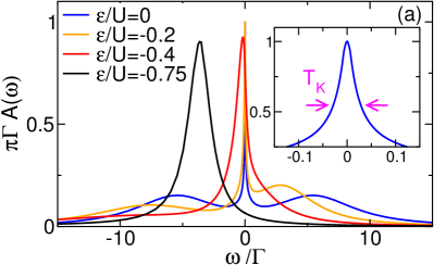
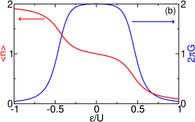
Figure 1: (a) Main plot: The single-particle dot spectral function for $U/\Gamma=4\pi$ and different level positions. Inset: Zoom-in of the spectral function at $\epsilon=0$. (b) The level occupancy (left scale) and the linear conductance (right scale) as a function of $\epsilon$. The NRG data were provided by T. Pruschke.

For vanishing Zeeman field the (Matsubara) dot Green function ${\mathcal{G}}_{\sigma}(i\omega)$ is spin independent and we suppress the spin index. The spectral function can be computed from the Green function analytically continued to real frequencies

$$A(\omega)=-\frac{1}{\pi}\mbox{Im}\,{\mathcal{G}}(\omega+i0).$$ (20)

In Fig. 1 (a) we show the $T=0$ dot single-particle spectral function of the SIAM (with metallic leads) for $U/\Gamma=4\pi$ and different $\epsilon$ obtained by NRG. We here do not give any details on the NRG approach as they can be found in the review [5]. We merely note that it provides highly accurate numerical low-energy results for a variety of important observables of the SIAM (as well as of other quantum impurity models) in equilibrium, provided the two numerical parameters–the logarithmic discretization parameter $\Lambda$ and the number of states $N_{\rm c}$ kept–are properly chosen. The results at higher energies are not as accurate, which, however, does not play a significant role for our purposes. Applying NRG it is also possible to gain direct physical insights, e.g., about the low-energy fixed point structure. This will turn out to be important when extracting the phase diagram for the SIAM with BCS leads. The Kondo effect leads to a sharp resonance of width $T_{\rm K}\ll\Gamma$–the latter being the width for $U=0$–which is pinned to the Fermi level (at $\omega=0$) when varying $\epsilon$; see Fig. 1 (a). This Kondo temperature scales exponentially in $U/\Gamma$. One often refers to the analytic expression

$$T_{\rm K}^{\rm ana}=\sqrt{U\Gamma/2}\exp{\left(-\frac{\pi}{8U\Gamma}\left|U^{2}-4\epsilon^{2}\right|\right)}$$ (21)

extracted from the susceptibility of the local spin computed from the Bethe ansatz solution of the SIAM.[6, 3] However, a few words of caution are in order with respect to the use of this formula. (i) The prefactor of the exponential function depends on the observable studied. This concerns parameter dependencies as well as numerical factors. (ii) Even ignoring this prefactor issue Eq. (21) should only be used deep in the Kondo regime when the absolute value of the argument of the exponential function is much larger than 1. Importantly, the extreme Kondo limit is not reached in most experiments; see Sect. 3. Besides the Kondo resonance the spectral function for $\epsilon\approx 0$ shows two Hubbard bands roughly located at $\pm U/2$.

At $T=0$ the linear conductance $G$ (infinitesimal bias voltage) depends on the spectral function at the Fermi energy and is given by[13]

$$G=4\Gamma_{L}\Gamma_{R}A(0)/\Gamma.$$ (22)

The pinning of the spectral weight at $\omega=0$ thus leads to a plateau (Kondo ridge) in $G$ with width of the order of $U$ if $\epsilon$ is varied around $0$. This is shown in Fig. 1 (b) (solid blue line) which in addition contains data for the dot occupancy (solid red line). The latter follows by integrating $A(\omega)$ over frequency up to the Fermi energy at $\omega=0$. The pinning of the resonance leads to a plateau of the dot occupancy at 1/2. We note that while the dot Green function and thus the dot spectral function (and the dot occupancy) only depends on $\Gamma=\Gamma_{L}+\Gamma_{R}$, due to the above prefactor $4\Gamma_{L}\Gamma_{R}/\Gamma$ the conductance is in addition sensitive to the left-right asymmetry $a=\Gamma_{L}/\Gamma_{R}\neq 1$. The Kondo effect is destroyed by temperatures $T>T_{\rm K}$ or Zeeman splittings $\left|\epsilon_{\uparrow}-\epsilon_{\downarrow}\right|>T_{\rm K}$. Both degrade the conductance plateau and lead to a local minimum of $G(\epsilon)=G_{\uparrow}(\epsilon)+G_{\downarrow}(\epsilon)$ at $\epsilon=0$. We will return to this in Sect. 3.

Standard techniques such as perturbation theory in $U$ or $\Gamma$, or the mean-field approximation[14] do not capture the Kondo effect in the SIAM (no Kondo peak of exponentially small width in $A(\omega)$, no conductance plateau in $G$). Within the unrestricted mean-field approach the spin-symmetry is spuriously broken in roughly the parameter regime in which the Kondo effect can be observed.[15] This is a rather fundamental deficit of the unrestricted mean-field approximation which renders it an inappropriate tool to study correlated quantum dots. As discussed below the same holds if the metallic leads are replaced by superconducting ones.

1.2.2 Superconducting leads

BCS superconductivity requires the formation of Cooper pairs of opposite spin (and momentum). Thus, scattering off magnetic impurities will affect superconductivity. This was investigated already at the end of the 50’ties and beginning of the 60’ties in models describing bulk BCS superconducting electrons interacting with a single or a few localized spin-1/2 degrees of freedom ignoring charge fluctuations and Kondo physics (see, e.g., Ref. [16]). Shortly after Kondo’s seminal work the interplay of the Kondo effect and superconductivity was investigated by several authors employing a Kondo model description of the localized spin (suppressed charge fluctuation).[17, 18, 19] It was shown that the superconducting gap acquires the logarithmic temperature dependence as described by Kondo for the resistance of a metallic host.[4] Note that at that time neither NRG and QMC nor the Bethe ansatz solution were available which limited the insights which could be gained. Furthermore, the Kondo model with a BCS reservoir was considered in its own right but not derived from the SIAM. In fact, only later it became apparent that a generalized Schrieffer-Wolff transformation leads to additional terms not present for a metallic reservoir.[20]

In parallel the effect of a classical spin in a superconductor was studied.[21, 22, 23] In such systems a pair of bound states with energies located in the superconducting gap forms which is nowadays referred to as Yu-Shiba-Rusinov states. The appearance of a pair of in-gap states at energies symmetrically located around the Fermi energy was also investigated for quantum spins, i.e., within the Kondo model with BCS leads.[19, 24, 25] It was found that the energies of these bound states move when varying the ratio $T_{\rm K}/\Delta$ and that their nature changes from being a singlet for $T_{\rm K}/\Delta\ll 1$ to being a doublet for $T_{\rm K}/\Delta\gg 1$.[26] This provided a first indication that a ground state level crossing (first order quantum phase transition) might occur for $T_{\rm K}/\Delta\approx 1$ between a doublet for $T_{\rm K}/\Delta\ll 1$ and a singlet for $T_{\rm K}/\Delta\gg 1$. At the transition the first excited in-gap state becomes the ground state and vice versa, that is the bound states reach the Fermi energy at this point. However, due to restrictions of the applicability of the methods used in the two limits of very large and very small $T_{\rm K}/\Delta$ no comprehensive understanding was achieved at that time. The results are in accordance with the physical picture that for $T_{\rm K}/\Delta\ll 1$ superconductivity prevails, the Kondo singlet cannot develop and the spin becomes free (doubly degenerate). In contrast for $T_{\rm K}/\Delta\gg 1$ the Kondo effect prevails and the spin is screened to form a (modified) Kondo singlet. This level crossing scenario and the associated change of the ground state degeneracy was unambiguously confirmed only two decades later when NRG was first applied to the Kondo model with BCS leads in 1992.[27, 28] In none of the above works a finite phase difference $\phi$ of the superconducting order parameter was considered. In bulk systems with embedded spin-1/2 degrees freedom the notion of a phase difference across the impurity is meaningless.

In the expressions of the last paragraph $T_{\rm K}$ refers to the Kondo temperature as it would emerge in the system after setting $\Delta=0$; we will refer to it as the normal state $T_{\rm K}$. For finite $\Delta$, and in particular for $\Delta$ larger than the normal state $T_{\rm K}$ one cannot expect that an inherent Kondo scale emerges; the Kondo effect does not (fully) develop. This indicates that in the interesting transition region from Kondo to superconductivity dominated behavior the ratio $T_{\rm K}/\Delta$ might not be the relevant parameter. The assumption that this ratio is the only relevant variable to characterize observables (“Kondo universality”) becomes even more questionable if the SIAM (including charge fluctuations) instead of the Kondo model is used; see Sect. 2.

The tunneling of Cooper pairs leads to the Josephson current. Magnetic impurities (localized spin-1/2 degrees of freedom) in the barrier separating the two superconductors will thus alter this equilibrium current. A reduction of the current and potentially even a sign change was predicted ignoring the Kondo effect by Kulik in 1966.[29, 30] The supercurrent in the presence of Kondo’s logarithmic corrections to the scattering was computed shortly after.[31] Further indications of possible $\pi$-junction behavior were given in Ref. [32]. The strong effect of the level-crossing transition discussed in the second to last paragraph on the Josephson current was only studied much later and will be one of the main topics of the rest of this review.

As mentioned above to give a full account of the physics of a correlated single-level quantum dot with two superconducting leads and to be in a position to compare to recent experiments we need to include charge fluctuations and thus to study the SIAM with BCS leads as a minimal model. In the next section we discuss the physics of this model and briefly account for the historic development (as we just did for the Kondo model with superconducting leads) in Subsects. 2.4 and 2.5.

2 A minimal model and its physics

2.1 The model

The Hamiltonian of a minimal model for transport through a single-level dot with two BCS leads including charge fluctuations can be obtained by adding the terms of Eqs. (1), (18), and (19). The direct hopping between the superconducting leads Eq. (2) is considered in addition in Subsect. 4.1.

In a first step we also rewrite $H_{\rm dot}$ and $H_{\rm coup}^{s}$ in terms of the Nambu spinor Eq. (5) and

$$\varphi=\left(\begin{array}[]{c}d^{\phantom{{\dagger}}}_{\uparrow}\\ d^{{\dagger}}_{\downarrow}\end{array}\right)$$ (25)

as

$$H_{\rm dot}=\epsilon\varphi^{\dagger}\sigma_{3}\varphi^{\phantom{{\dagger}}}-U\left(\varphi_{1}^{\dagger}\varphi_{1}^{\phantom{{\dagger}}}-1/2\right)\left(\varphi_{2}^{\dagger}\varphi_{2}^{\phantom{{\dagger}}}-1/2\right)$$ (26)

and

$$H_{\rm coup}^{s}=-t_{s}\Psi^{\dagger}_{s}\sigma_{3}\varphi^{\phantom{{\dagger}}}+\mbox{H.c.},$$ (27)

still assuming a spin-degenerate level $\epsilon_{\uparrow}=\epsilon=\epsilon_{\downarrow}$. Using the equation-of-motion technique we can compute the $U=0$ (Nambu space Matsubara) dot Green function including the lead self-energy

$${\mathcal{G}}_{0}(i\omega)=\frac{-1}{D_{0}(i\omega)}\left(\begin{array}[]{cc}i\tilde{\omega}+\epsilon&-\tilde{\Delta}\\ -\tilde{\Delta}^{\ast}&i\tilde{\omega}-\epsilon\end{array}\right),\quad D_{0}(i\omega)={\tilde{\omega}}^{2}+\epsilon^{2}+\left|\tilde{\Delta}\right|^{2},$$ (30)

with

$$i\tilde{\omega}=i\omega\left(1+\frac{\Gamma}{\sqrt{\omega^{2}+\Delta^{2}}}\right),\quad\tilde{\Delta}=\Delta\sum_{s}\frac{\Gamma_{s}}{\sqrt{\omega^{2}+\Delta^{2}}}e^{i\phi_{s}}.$$ (31)

The anomalous off-diagonal terms of the dot Green function are signatures of the proximity effect. The full interacting dot Green function is obtained as

$${\mathcal{G}}(i\omega)=\frac{-1}{D(i\omega)}\left(\begin{array}[]{cc}i\tilde{\omega}+\epsilon+\Sigma^{\ast}(i\omega)&-\tilde{\Delta}+\Sigma_{\Delta}(i\omega)\\ -\tilde{\Delta}^{\ast}+\Sigma_{\Delta}^{\ast}(i\omega)&i\tilde{\omega}-\epsilon-\Sigma(i\omega)\end{array}\right),$$ (34)

with

$$D(i\omega)=\tilde{\omega}^{2}+\left|\epsilon+\Sigma(i\omega)\right|^{2}+\left|\tilde{\Delta}-\Sigma_{\Delta}(i\omega)\right|^{2},$$ (35)

were a form of the self-energy matrix $\mathcal{S}$ (resulting from the local interaction) was used which obeys all symmetries (including those which follow from spin-symmetry)[33, 34]

$$\mathcal{S}(i\omega)=\left(\begin{array}[]{cc}\Sigma(i\omega)&\Sigma_{\Delta}(i\omega)\\ \Sigma_{\Delta}^{\ast}(i\omega)&-\Sigma^{\ast}(i\omega)\end{array}\right).$$ (38)

The relevant part of the current operator is now obtained from the commutator $\left[H_{\rm coup}^{s},\hat{N}_{s}\right]$ and will be denoted by $\hat{J}_{s}^{\rm imp}$. It reads

$$\hat{J}_{s}^{\rm imp}=-it_{s}\varphi^{\dagger}_{\phantom{s}}\Psi_{s}^{\phantom{{\dagger}}}+\mbox{H.c.}.$$ (39)

Its thermal expectation value can thus be expressed in terms of the lead-dot Green function ${\mathcal{G}}_{s,{\rm d}}(i\omega)$ as

$$J_{s}^{\rm imp}=\frac{2t_{s}}{\beta}\sum_{i\omega}\mbox{Im}\,\mbox{Tr}\,{\mathcal{G}}_{s,{\rm d}}(i\omega).$$ (40)

The contribution to the current from the commutator of $H_{\rm lead}^{s}$ with $\hat{N}_{s}$ again vanishes due to the BCS self-consistency condition (see Subsect. 1.1). Employing the equation-of-motion approach the lead-dot Green function can be written in terms of the full dot Green function as

$${\mathcal{G}}_{s,{\rm d}}(i\omega)=-t_{s}g_{s}(i\omega)\sigma_{3}{\mathcal{G}}(i\omega).$$ (41)

In turn the current can be computed as

$$J_{s}^{\rm imp}=\frac{-2t_{s}^{2}}{\beta}\sum_{i\omega}\mbox{Im}\,\mbox{Tr}\,\left[g_{s}(i\omega)\sigma_{3}{\mathcal{G}}(i\omega)\right].$$ (42)

Inserting Eqs. (34) and (15) this leads to an explicit expression for the Josephson current which involves the self-energy

$$J_{s}^{\rm imp}=\frac{4}{\beta}\sum_{i\omega}\left\{\frac{\Gamma_{s}\Gamma_{\bar{s}}\Delta^{2}}{\omega^{2}+\Delta^{2}}\frac{\sin\left(\phi_{s}-\phi_{\bar{s}}\right)}{D(i\omega)}-\frac{\Gamma_{s}\Delta\left[e^{i\phi_{s}}\Sigma_{\Delta}^{\ast}(i\omega)-e^{-i\phi_{s}}\Sigma_{\Delta}^{\phantom{\ast}}(i\omega)\right]}{2iD(i\omega)\sqrt{\omega^{2}+\Delta^{2}}}\right\}.$$ (43)

The diagonal entry $\Sigma(i\omega)$ of the self-energy matrix enters only via $D(i\omega)$ Eq. (35).

We merely note that within an exact treatment of the model the supercurrent is conserved: $J_{L}^{\rm imp}=-J_{R}^{\rm imp}$. In case the self-energy is computed approximately it depends on the approximation scheme whether or not current conservation holds. For a discussion of this for the Anderson-Josephson dot, see, e.g., Ref. [34]. All results shown in this review were obtained by methods which obey current conservation and we will only consider $J_{L}^{\rm imp}$ from now on.

The current can equivalently be computed as twice the derivative of the free energy with respect to the relative phase $\phi$. We show this for the Hamiltonian $H(\phi_{L},\phi_{R})=H_{\rm lead}^{L}(\phi_{L})+H_{\rm lead}^{R}(\phi_{R})+H_{\rm dot}+H_{\rm coup}^{L}+H_{\rm coup}^{R}+H_{\rm direct}$ Eqs. (1), (18), (19), and (2) including a direct hopping between the two superconductors given by $H_{\rm direct}$; see Subsect. 4.1. To this end we perform a gauge transformation

$$c_{s,k,\sigma}\to e^{-i\phi_{s}/2}c_{s,k,\sigma},\quad d_{\sigma}\to e^{-i\phi_{R}/2}d_{\sigma}$$ (44)

after which $H$ can be rewritten as

$$\bar{H}(\phi)= H_{\rm lead}^{L}(\phi_{L}=0)+H_{\rm lead}^{R}(\phi_{R}=0)+H_{\rm dot}$$

$$+H_{\rm coup}^{L}(t_{L}\to\bar{t}_{L})+H_{\rm coup}^{R}+H_{\rm direct}(t_{\rm d}\to\bar{t}_{\rm d}),$$ (45)

with $\bar{t}_{L}=e^{-i\phi/2}t_{L}$ and $\bar{t}_{\rm d}=e^{-i\phi/2}t_{\rm d}$ in self-explaining notation. The sum of the two current operators Eqs. (11) and (39) (with $s=L$) can then be obtained by taking the derivative

$$\hat{J}_{L}=2\partial_{\phi}\left[H_{\rm coup}^{L}(t_{L}\to\bar{t}_{L})+H_{\rm direct}(t_{\rm d}\to\bar{t}_{\rm d})\right]=2\partial_{\phi}\bar{H}(\phi).$$ (46)

Exploiting the Hellmann-Feynman theorem this leads to

$$J_{L}=2\partial_{\phi}\Omega(\phi),$$ (47)

with the free energy $\Omega$. Obviously, this relation also holds if either the coupling via the dot or via the direct link are set to zero; for now we will again focus on the latter case. These considerations also show explicitely that the supercurrent is only a function of the relative phase $\phi=\phi_{L}-\phi_{R}$; the average phase $\eta=(\phi_{L}+\phi_{R})/2$ does not enter, a property which is rooted in the gauge invariance of the current.

In the past it was generally believed that the case of left-right symmetric couplings with $a=\Gamma_{L}/\Gamma_{R}=1$ does not contain all informations to fully understand the more general asymmetric one with $a\neq 1$. However, in a recent important work Kadlecová, Žonda, and Novotný showed that typical observables such as, e.g., the free energy, the dot occupancy, and the current of a general asymmetric system can be computed from the corresponding expressions obtained for the symmetric case.[36] For the current at given asymmetry $a$ and phase difference $\phi$ the exact transformation reads

$$J_{L}^{\rm imp}(\phi)= \frac{\cos(\phi/2)}{\sqrt{\frac{(a+1)^{2}}{4a}-\sin^{2}(\phi/2)}}$$

$$\times J_{L}^{\rm imp,sym}\left(2\arccos\sqrt{1-\frac{4a}{(a+1)^{2}}\sin^{2}[\phi/2]}\right),$$ (48)

with $J_{L}^{\rm imp,sym}(\psi)$ being the expression for the supercurrent at relative phase $\psi$ obtained in the symmetric case $a=1$.

This has practical implications. In experimental setups it is nearly impossible to reach $a=1$. For a comparison still, only the current for $a=1$ has to be computed which can then be transformed according to the experimental asymmetry; the parameter space is effectively reduced by one dimension. However, the above insight also has fundamental consequences. As discussed in Subsect. 1.2 in the past it was often presumed that observables only depend on the ratio $T_{\rm K}/\Delta$ provided the system parameters for suppressed superconductivity are chosen such that the dot is in the Kondo regime. In systems with metallic leads a similar exclusive dependence on $T_{\rm K}/S$, with $S$ being an energy scale of the system (e.g. the temperature), is referred to as “Kondo universality”. The supposed scaling in $T_{\rm K}/\Delta$ was used in theoretical as well as in experimental investigations of dots with superconducting leads. While according to Eq. (2.1) the supercurrent changes with varying asymmetry $a$ at fixed $\Gamma=\Gamma_{L}+\Gamma_{R}$ the ratio $T_{\rm K}/\Delta$ remains invariant, as $T_{\rm K}$ only depends on $\Gamma$; see Eq. (21). The same holds for other observables. This provides a more clear-cut argument that this type of “Kondo universality” is of minor relevance for the Anderson-Josephson quantum dot than the somewhat vague one given in Subsect. 1.2.

2.2 The $U=0$ Josephson current

For $U=0$ the self-energy $\mathcal{S}$ vanishes. For $T=0$ and $\Gamma_{L}=\Gamma/2=\Gamma_{R}$ (without loss of generality, see the second to last paragraph of Subsect. 2.1) the left current can then be written as

$$J_{L}^{\rm imp} =\frac{\sin(\phi)}{2\pi}\int_{-\infty}^{\infty}d\omega\frac{\Gamma^{2}\Delta^{2}}{\Gamma^{2}\Delta^{2}\cos^{2}(\phi/2)+\omega^{2}\left(\Gamma+\sqrt{\omega^{2}+\Delta^{2}}\right)^{2}+\epsilon^{2}\left(\omega^{2}+\Delta^{2}\right)}$$

$$=\frac{\Delta\sin(\phi)}{2\pi}\int_{-\infty}^{\infty}dx\frac{1}{\cos^{2}(\phi/2)+x^{2}\left(1+\frac{\Delta}{\Gamma}\sqrt{x^{2}+1}\right)^{2}+\left(\frac{\epsilon}{\Gamma}\right)^{2}\left(x^{2}+1\right)}.$$ (49)

The supercurrent is a $2\pi$-periodic odd function of $\phi$. This also holds for $U>0$, which can, e.g., be inferred from Eq. (47) and implies that later on we can restrict our attention to $\phi\in[0,\pi]$.

For $|\epsilon|/\Gamma\gg 1$ all but the last term in the denominator of the integrand can be neglected. The integral can then be performed leading to

$$J_{L}^{\rm imp}=\Delta\frac{\sin(\phi)}{2}\left(\frac{\Gamma}{\epsilon}\right)^{2},\quad\frac{|\epsilon|}{\Gamma}\gg 1.$$ (50)

As expected the CPR for a noninteracting dot with a large onsite energy becomes purely sinusoidal as it is the case for the current through a weak link connecting two superconductors; compare Eq. (17). For small $|\epsilon|/\Gamma$, i.e., close to the transport resonance, the internal degree of freedom of the dot matters and higher harmonics affect the CPR. This can analytically be seen in the limit of either $\Delta/\Gamma\ll 1$ or $\Delta/\Gamma\gg 1$ in which

$$J_{L}^{\rm imp}=\frac{\sin(\phi)}{2\sqrt{\left(\frac{\epsilon}{\Gamma}\right)^{2}+\cos^{2}(\phi/2)}}\times\left\{\begin{array}[]{l}\Delta\quad\mbox{for}\,\frac{\Delta}{\Gamma}\ll 1,\frac{|\epsilon|}{\Gamma}\ll 1\\ \Gamma\quad\,\mbox{for}\,\frac{\Delta}{\Gamma}\gg 1,\frac{|\epsilon|}{\Gamma}\ll 1\end{array}\right.$$ (53)

For $\epsilon=0$ the Josephson current is proportional to $\pm\sin(\phi/2)$ with a sign change from $+$ to $-$ at $\phi=\pi$. For small $|\epsilon|/\Gamma$ the resulting jump at $\phi=\pi$ is smeared out as shown in Fig. 2 which displays $J_{L}^{\rm imp}/\Delta$ of Eq. (49) as a function of $\phi$ for various $\epsilon/\Gamma$. We took $\Delta/\Gamma=1/3$ which is roughly the value found in the experimental setups discussed in Sect. 3. On the scale of the plot the data for $\epsilon/\Gamma=2$ (green curve) are already indistinguishable from the large $\epsilon$ result Eq. (50).

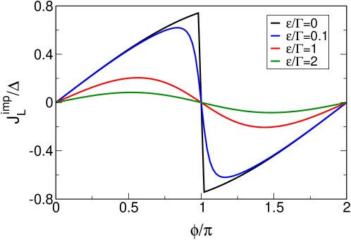
Figure 2: Noninteracting ($U=0$) zero-temperature Josephson current $J_{L}^{\rm imp}$ as a function of the phase difference $\phi$ Eq. (49) for $\Delta/\Gamma=1/3$ and different $\epsilon$.

After analytic continuation from Matsubara to real frequencies the noninteracting Green function Eq. (30) has a pair of poles (zeros of the determinant $D_{0}$) located symmetrically around zero at energies inside the interval $[-\Delta,\Delta]$. They correspond to many-body states which are commonly referred to as Andreev bound states and indicated by in-gap $\delta$-peaks in the single-particle spectral function. Employing the Lehmann representation of the lesser (photoemission) and greater (inverse photoemission) spectral function it is obvious that the absolut value of the bound state energy corresponds to the energy difference between the many-body ground state and first excited one. Although the spectral properties are not at the focus of our attention it is still interesting to investigate if these bound states survive for $U>0$ and if so, how they are related to the Yu-Shiba-Rusinov states obtained in spin models.[37] We therefore comment on the bound states when appropriate.

2.3 The infinite gap limit: exact solution

To gain insights into the physics for $U>0$ we first consider the limit $\Delta\to\infty$ (atomic limit). As indicated in the last subsection this is not the limit as realized in systems of experimental interest. However, it allows us to obtain the exact solution analytically. We note that by first discussing the $\Delta\to\infty$ limit of the $U>0$ SIAM with BCS leads we do not follow the historic development. In fact, this limit was considered at a surprisingly late stage.[38, 39] We here consider the general case with asymmetry $a\neq 1$ as this does not cause any additional difficulties.

For $\Delta\to\infty$ the noninteracting dot Green function simplifies to [see Eqs. (30) and (31)]

$${\mathcal{G}}_{0}^{-1}(i\omega)=\left(\begin{array}[]{cc}i\omega-\epsilon&\Delta_{\rm d}\\ \Delta^{\ast}_{\rm d}&i\omega+\epsilon\end{array}\right),\quad\Delta_{\rm d}=\sum_{s}\Gamma_{s}e^{i\phi_{s}}.$$ (56)

It is now obvious that all system properties which can be studied based on $\mathcal{G}$, that is ${\mathcal{G}}_{0}$ via a perturbative expansion, can be computed considering the effective Hamiltonian

$$H_{\rm atom}=\epsilon\left(\varphi^{\dagger}_{1}\varphi^{\phantom{{\dagger}}}_{1}-\varphi^{\dagger}_{2}\varphi^{\phantom{{\dagger}}}_{2}\right)-\Delta_{\rm d}\varphi^{\dagger}_{1}\varphi^{\phantom{{\dagger}}}_{2}-\Delta_{\rm d}^{\ast}\varphi^{\dagger}_{2}\varphi^{\phantom{{\dagger}}}_{1}-U\left(\varphi_{1}^{\dagger}\varphi_{1}^{\phantom{{\dagger}}}-1/2\right)\left(\varphi_{2}^{\dagger}\varphi_{2}^{\phantom{{\dagger}}}-1/2\right).$$ (57)

This includes the current and the eigenenergies as well as their degeneracy. In the many-particle basis $\left\{\left|0,0\right>,\left|1,0\right>,\left|0,1\right>,\left|1,1\right>\right\}$ (in self-explaining notation) it is represented by the matrix

$${\mathcal{H}}_{\rm atom}=\left(\begin{array}[]{cccc}-U/4&0&0&0\\ 0&U/4+\epsilon&-\Delta_{\rm d}&0\\ 0&-\Delta_{\rm d}^{\ast}&U/4-\epsilon&0\\ 0&0&0&-U/4\end{array}\right)$$ (62)

The single-particle $2\times 2$-block can easily be diagonalized leading to the eigenvalues $U/4\pm\sqrt{\epsilon^{2}+|\Delta_{\rm d}|^{2}}$. The ground state is thus nondegenerate (doubly-degenerate) if

$$U/4-\sqrt{\epsilon^{2}+|\Delta_{\rm d}|^{2}}\lessgtr-U/4\quad\Leftrightarrow\quad U/2\lessgtr\sqrt{\epsilon^{2}+|\Delta_{\rm d}|^{2}}.$$ (63)

with

$$|\Delta_{\rm d}|^{2}=\Gamma_{L}^{2}+\Gamma_{R}^{2}+2\Gamma_{l}\Gamma_{R}\cos\phi.$$ (64)

The opposite holds for the first excited state. One can conclude that a ($T=0$) level-crossing quantum phase transition between a singlet and a doublet ground state can be driven by varying $U$, $\epsilon$, $\Gamma_{s}$ or $\phi$ if the other parameters are taken from appropriate ranges. For properly chosen fixed $U$, $\epsilon$, $\Gamma=\Gamma_{L}+\Gamma_{R}$, and $a=\Gamma_{L}/\Gamma_{R}$ Eq. (63) defines a critical phase difference $\phi_{\rm c}\in[0,\pi]$ at which the transition from the singlet to the doublet state takes place. Alternatively, a critical interaction $U_{\rm c}$, a critical level position $\epsilon_{\rm c}$, a critical tunneling rate $\Gamma_{\rm c}$, or a critical asymmetry $a_{\rm c}$ can be defined.

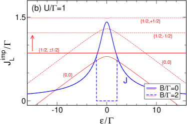
Figure 3: Gate voltage $\epsilon$ dependence of the Josephson current (blue lines) as well as of the three lowest many-particle energies (red lines) in the large-gap limit $\Delta\to\infty$ at phase difference $\phi/\pi=1/2$, different Coulomb interactions $U$, and Zeeman fields $B$. The many-particle energies are shown in arbitrary units; those for finite $B$ (dashed lines) were shifted upwards for clarity as indicated by the arrow. The corresponding eigenstates are characterized by spin quantum numbers $\{s,m\}$. Reprinted figure with permission from C. Karrasch, S. Andergassen, and V. Meden, Phys. Rev. B 84, 134512 (2011). Copyright (2011) by the American Physical Society.

To further illustrate this it is useful to compute the spin quantum numbers $\{s,m\}$ of the states. The spin operator is defined as $\hat{\vec{s}}=\sum_{\sigma,\sigma^{\prime}}d_{\sigma}^{\dagger}\vec{\sigma}_{\sigma,\sigma`}d_{\sigma^{\prime}}$, with $\vec{\sigma}$ being the vector of Pauli matrices. It is straightforward to show that $\hat{\vec{s}}^{2}$ and $\hat{s}_{3}$ commute with each other as well as with $H_{\rm atom}$. In Fig. 3 the $\epsilon$ dependence of the energy of the three lowest lying many-body states is shown for $a=1$, $\phi=\pi/2$ and two different $U/\Gamma$. The solid red lines are labeled by their spin quantum numbers. In Fig. 3 (a) $U/\Gamma$ is sufficiently large such that a level crossing from the $\{s=0,m=0\}$ singlet to the $\{s=1/2,m=\pm 1/2\}$ doublet occurs around $\epsilon/\Gamma=\pm 4$ , while for the smaller $U/\Gamma$ in (b), the singlet is the ground state for all $\epsilon$.

One can straightforwardly extend the exact solution to the case with a Zeeman field of amplitude $B$ and level energies $\epsilon_{\uparrow}=\epsilon+B$, $\epsilon_{\downarrow}=\epsilon-B$ by replacing $\epsilon$ in the $(1,1)$-matrix element of Eq. (56) by $\epsilon+B$ as well as $\epsilon\to\epsilon-B$ in the $(2,2)$-matrix element and accordingly in the steps leading to the equation for the phase boundary. The levels for this case are shown as dashed red lines in Fig. 3. This shows that even for small $U/\Gamma$ a level crossing phase transition can be induced by a sufficiently large Zeeman field; see Fig. 3 (b). However, the transition is no longer one between a nondegenerate and a (almost) doubly-degenerate state. For small enough $B$ at large $U/\Gamma$ [dashed lines in Fig. 3 (a)] the physics is still determined by the interplay of one nondegenerate $\{s=0,m=0\}$ state and a pair of almost twofold-degenerate ones $\{s=1/2,m=\pm 1/2\}$. Further down we will return to these observations.

The first excited state of the present $\Delta\to\infty$ limit mimics the in-gap Andreev bound states discussed in the last subsection for $U=0$; the continuum was shifted to $\pm\infty$. Varying the parameters the bound state energy moves and hits zero at the transition. Approaching the transition from the singlet side at this point the singlet ground state and the doublet first excited state become degenerate; the excitation energy given by the bound state energy vanishes. Beyond the transition (in the doublet phase) the doublet is the ground state and has a finite energy gap to the first excited singlet. This is the same phenomenology as observed for the Yu-Shiba-Rusinov states in the Kondo model with BCS leads (see Subsect. 1.2) and again raises the question about the relation of these and the Andreev bound states.[37]

As reviewed in Subsect. 1.2 for the Kondo model with superconducting leads and discussed below for the SIAM the transition between a singlet and doublet ground state does not only occur for $\Delta\to\infty$ but also for generic $\Delta$. This type of physics is absent at $U=0$ and can thus be directly linked to the two-particle interaction (the exchange interaction in the Kondo model with BCS leads). However, for $\Delta\to\infty$ the Kondo effect is suppressed completely and it can thus not be assigned as the driving force for such a transition. For finite $\Delta$ remnants of the Kondo effect can, however, be expected to affect the transition. We investigate this in the next subsection.

The simplest way to obtain the Josephson current in the atomic limit at $T=0$ is to take the derivative of the many-body ground state energy with respect to $\phi$ [see Eq. (47)]. This leads to

$$J_{L}^{\rm imp}=\left\{\begin{array}[]{ll}\frac{2\Gamma_{L}\Gamma_{R}\sin\phi}{\sqrt{\epsilon^{2}+\Gamma_{L}^{2}+\Gamma_{R}^{2}+2\Gamma_{L}\Gamma_{R}\cos\phi}},&\mbox{singlet phase}\\ 0,&\mbox{doublet phase}\end{array}\right.$$ (67)

Note that the current in the singlet phase is equal to the $U=0$ current; compare to the lower line of Eq. (53) for $\Gamma_{L}=\Gamma/2=\Gamma_{R}$. Equivalently, the interacting dot Green function and thus the self-energy can be computed using the Lehmann representation.[35] From this the current can be obtained performing the frequency integral of Eq. (43). Equation (67) shows that the ($T=0$) quantum phase transition (resulting from the two-particle interaction) is indicated by a jump of the supercurrent from a finite value to zero. The $\epsilon$ dependence of the current is shown as the blue lines in Fig. 3. The vanishing of the current in the doublet phase is special to the atomic limit. However, the jump is also found for generic $\Delta$ as discussed next. In this case the current in the doublet phase is negative even for $\phi\in[0,\pi]$; compare to the $U=0$ current of Fig. 2 which is positive for $\phi\in[0,\pi]$. For this reason one speaks interchangeably of the doublet- or $\pi$-phase and the singlet- or $0$-phase. The jump of the current as a function of $\phi$ at $\phi_{\rm c}<\pi$ (for properly chosen fixed $U$, $\epsilon$, $\Gamma$, and $a$) resulting from the quantum phase transition should not be confused with the jump at $\phi=\pi$ obtained for $U=0$ and $\epsilon=0$; see Subsect. 2.2, in particular the black curve in Fig. 2. Figure 3 shows that the line shape $J_{L}^{\rm imp}(\epsilon)$ resulting from the Zeeman field induced level crossing transition at small $U/\Gamma$ [see Fig. 3 (b)] resembles the one resulting from the transition induced by the two-particle interaction at $B=0$ [see Fig. 3 (a)].

2.4 “Nearly” exact results from elaborate quantum many-body methods

The expected equivalence of the SIAM with BCS leads to the Kondo model with such leads in the proper limit of large $U/\Gamma$ as well as $-U/2<\epsilon<U/2$ and the results for the latter model reviewed in Subsect. 1.2 suggest that the level crossing scenario of the $\Delta\to\infty$ limit survives at finite $\Delta$. In this subsection we show this based on NRG and QMC results. We discuss the phase diagram as well as the Josephson current and briefly the bound states.

The SIAM with two BCS leads and $\Delta<\infty$ was first treated by the NRG in Ref. [37]. Focusing on selected parameter sets, in particular $\phi=0$ and thus a vanishing Josephson current, the level crossing scenario was unambiguously confirmed. The assumed left-right symmetry and vanishing of the phase difference allowed the authors to reduce the problem to one with a single lead (single-channel NRG) which renders the NRG computationally less demanding. Analyzing the first few low-energy many-body states it was shown that increasing $U$ at fixed $\epsilon$ and $\Gamma$ leads to a groundstate crossing from a singlet to a doublet.

Figure 4 shows the phase diagram extracted from the low-energy spectra obtained by NRG (blue symbols connected by lines) as a function of $U/\Delta$ and $\Gamma_{R}/\Delta$. Two parameter sets as given in the figure are considered–including one with $\Gamma_{L}\neq\Gamma_{R}$ and $\phi\neq 0$. The data are taken from Ref. [35]. They fully confirm the $\Delta\to\infty$ scenario. A systematic study shows that decreasing $U$, $\epsilon$, $|a-1|$ or $\phi$ favors the singlet phase. To avoid a reproduction of the NRG data at a later stage of this review we included results obtained by an approximate FRG approach to be discussed in Subsect. 2.6 as red lines in Fig. 4.

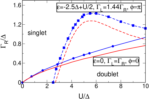
Figure 4: Phase diagram of the Anderson-Josephson dot obtained by NRG (blue symbols connected by lines) as a function of $U/\Delta$ and $\Gamma_{R}/\Delta$. Results for two different sets of the other parameters, as indicated in the figure, are shown. For efficiency reasons we included data obtained by an approximate FRG approach to be discussed in Subsect. 2.6 as red lines. The data were taken from Fig. 2 and Fig. 3 (b) of Ref. [35].

To compute the current at $T=0$ a two-lead NRG was first employed in [40]. At the quantum phase transition–the $0$-to-$\pi$-transition–the current jumps from a positive value to a negative one even for $\phi\in[0,\pi]$; the current shows $\pi$-junction behavior. It, however, turned out that the data for the supercurrent presented in this paper are inaccurate; the amplitude is roughly a factor of two to small.[35] The most likely reason for this is an improper selection of the NRG numerical parameters $\Lambda$ and $N_{\rm c}$ (see Ref. [35]).

To avoid the numerical obstacles of two-channel NRG Oguri, Tanaka, and Hewson[41] (see also Ref. [39]) studied the model in the limit in which the gap of the left lead is sent to infinity, while the right one is kept finite. Again the level-crossing scenario was confirmed. In contrast to the case in which both the left and the right gaps are sent to infinity the current in the doublet phase was found to be nonvanishing and negative even for $\phi\in[0,\pi]$.

Figures 5 (a) and (b) show the Josephson current as a function of $\phi\in[0,\pi]$ for various parameter sets with $\epsilon=0$, $\Gamma_{L}=\Gamma_{R}$, and finite gaps $\Delta$ computed using two-channel NRG with properly chosen numerical parameters (circles connected by dashed lines).[35] In Fig. 5 (a) the interaction $U$ is fixed and $\Delta$ is varied; vice versa in Fig. 5 (b). Remind that the current is a $2\pi$-periodic and odd function of $\phi$ and can thus accordingly be extended to phases outside the shown range. The solid lines show FRG results; see Subsect. 2.6. In accordance with the $\Delta\to\infty$ limit the quantum phase transition is indicated by a jump of the supercurrent. For $\phi\in[0,\pi]$ the current is positive in the singlet phase and negative in the doublet one. The same behavior is found for $\epsilon\neq 0$. Results for $\Gamma_{L}\neq\Gamma_{R}$ can be obtained from the symmetric case using the transformation Eq. (2.1). In the caption of Fig. 5 we give the values of $T_{\rm K}$ [computed from Eq. (21)] such that it is possible to estimate the strength of the correlations for suppressed superconductivity for a given parameter set. We, however, reemphasize that the ratio $\Delta/T_{\rm K}$ plays a by far less relevant role than assumed in large parts of the literature of the Anderson-Josephson quantum dot. For details on the NRG procedure in particular the NRG numerical parameters $\Lambda$ and $N_{\rm c}$, see Ref. [35].

Figure 6 (a) shows NRG data for the CPR at different temperatures. The parameters of the blue curve in Fig. 5 (a) ($U/\Gamma=5.2$, $\Delta/\Gamma=0.37$) are considered. The jump at $T=0$ results from a quantum phase transition and is thus smeared out out for $T>0$. Additionally, the amplitude of the current is strongly suppressed with increasing $T$.[35]

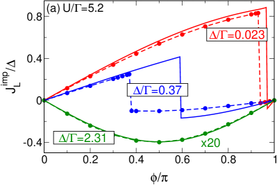
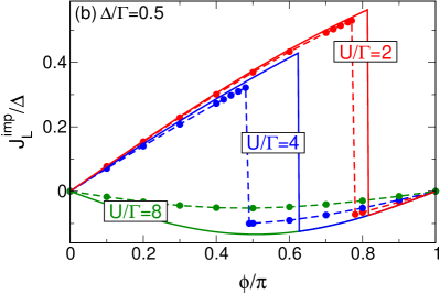
Figure 5: Zero-temperature Josephson current $J_{L}^{\rm imp}$ as a function of the phase difference $\phi$ computed with NRG (circles connected by dashed lines) and approximate FRG (solid lines) at $\epsilon=0$ and $\Gamma_{L}=\Gamma_{R}$. (a) $\Delta$ is varied at fixed $U/\Gamma=5.2$ ($T_{\rm K}/\Gamma=0.209$). For clarity, the curves at $\Delta/\Gamma=2.31$ were scaled up by a factor of $20$. (b) $\Delta/\Gamma=0.5$ is fixed at different $U/\Gamma$ corresponding to $T_{\rm K}/\Gamma=0.45$, $T_{\rm K}/\Gamma=0.29$, and $T_{\rm K}/\Gamma=0.09$. Reprinted figures with permission from C. Karrasch, A. Oguri, and V. Meden, Phys. Rev. B 77, 024517 (2008). Copyright (2008) by the American Physical Society.

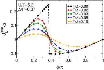
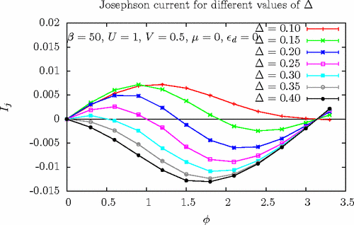
Figure 6: Finite-temperature Josephson current $J_{L}^{\rm imp}$ as a function of the phase difference $\phi$. Left panel: NRG data for the parameters of the blue curve of Fig. 5 (a). Reprinted figure with permission from C. Karrasch, A. Oguri, and V. Meden, Phys. Rev. B 77, 024517 (2008). Copyright (2008) by the American Physical Society. Right panel: CTINT QMC data for the left current $I_{j}$ ($=J_{L}^{\rm imp}$ in our notation). The parameters given in the figure must be translated to our model parameters as $V=t_{L}=t_{R}$ and $\epsilon_{d}=\epsilon$. In the CTINT QMC computation a lead band with dispersion $\epsilon_{k}=-2t\cos(k)$ is considered. Band effects can be neglected and the model becomes equivalent to the one in the wide band limit as long as all parameters of dimension energy, which here are given in units of $t$, are taken to be smaller than the hopping. Reprinted figure with permission from D.J. Luitz and F.F. Assaad, Phys. Rev. B 81, 024509 (2010). Copyright (2010) by the American Physical Society.

The supercurrent was also computed by the Hirsch-Fye QMC method[42] and the continuous-time interaction-expansion QMC (CTINT QMC) method,[43] both inherently being $T>0$ techniques. While the results of the first approach were shown to be accurate in the $T=0$ doublet phase but imprecise in the singlet one[35] the CTINT QMC approach of Ref. [43] leads to highly accurate (“nearly” exact) currents in both regimes. It was later used to directly compare to experimental data as reviewed in Sect. 3. The right panel of Fig. 6 shows CTINT QMC data at fixed $T$ for varying $\Delta$.[43].

A comprehensive NRG study of the $T=0$ spectral properties of the Anderson-Josephson quantum dot was presented in [44] (see also [45]). Figure 7 shows the (dot) spectral function at half filling of the dot ($\epsilon=0$) and for $\phi=0$ in the limit of a small gap on all relevant energy scales (left panel) and in a zoom-in on the scale of the gap (right panel). As the gap is small a Kondo resonance around $\omega=0$ starts to form with increasing $U$ and Hubbard bands develop; compare to the $\epsilon=0$-curve (blue) of Fig. 1. However, due to the superconductivity the spectral weight at low energies $|\omega|<\Delta$ is suppressed and the resonance does not fully develop. A symmetrically located pair of in-gap bound states appears which in Fig. 7 are shown as vertical arrows ($\delta$-peaks), the heights indicating the weight. Their position $E_{\rm b}$ and weight $w_{\rm b}$ depends on the parameters; in Fig. 7 on $U$. For increasing $U/\Gamma$ one crosses over from noninteracting Andreev bound states to the Yu-Shiba-Rusinov states both discussed above.

Figure 7: Dot spectral function at half dot filling $\epsilon=0$, vanishing phase $\phi=0$ for a small superconducting gap $\Delta=0.005D$ and coupling $\Gamma=0.2D/\pi$, with $D$ being half the lead band width. The lead density of states is assumed to be constant, but no wide band limit is taken. This fully corresponds to the model in the wide band limit as long as all parameters are taken to be smaller than $D$. The spectral function is computed by NRG and denoted as $\rho(\omega)$ (corresponding to $DA(\omega)$ in our notation). Left panel: Spectral weight on all relevant energy scales ($\omega$ is measured in units of $D$). Right panel: Zoom-in of the weight on the scale $\Delta_{\rm sc}$ ($=\Delta$ in our notation). The vertical arrows indicate $\delta$-peaks corresponding to in-gap bound states. Reprinted figure with permission from J. Bauer, A. Oguri, and A.C. Hewson, J. Phys.: Condens. Matter 19, 486211 (2007). Copyright (2007) by the Institute of Physics.

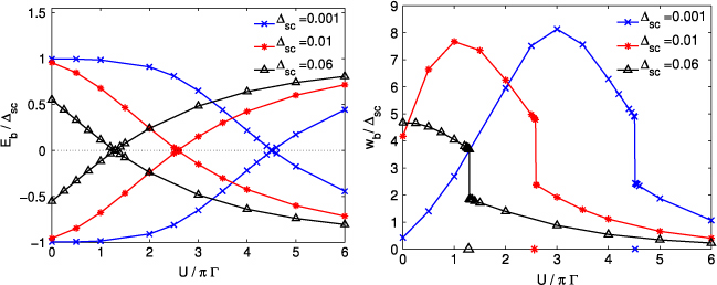
Figure 8: Parameter dependence of the position $E_{\rm b}$ (left panel) and the weight $w_{\rm b}$ (right panel) of the in-gap bound states. The symbols on the $x$-axis of the right panel indicate the position of the quantum phase transition (zeros of the left panel). The gap $\Delta_{\rm sc}$ ($=\Delta$ in our notation) is measured in units of $D$. The other parameters are $\epsilon=0$, $\phi=0$ and $\Gamma=0.2D/\pi$. Reprinted figure with permission from J. Bauer, A. Oguri, and A.C. Hewson, J. Phys.: Condens. Matter 19, 486211 (2007). Copyright (2007) by the Institute of Physics.

The parameter dependence of the bound states is further illustrated in Fig. 8 which shows $E_{\rm b}$ and $w_{\rm b}$ as a function of $U$ for different $\Delta$. In full accordance with the results for the Kondo model with BCS leads the energy of the pair of in-gap states hits zero at the quantum phase transition. The gap between the many-body ground state and the first excited one which is given by $\left|E_{\rm b}\right|$ vanishes. The first excited state becomes the ground state and vice versa. Note that the appearance of a pair of $\delta$-peaks is unrelated to the observation that one of the two involved states is a doublet but rather follows from the fact that the total spectral function shown contains the photoemission as well as the inverse photoemmission part. In addition, the weight of the $\delta$-peaks depends on the parameters and jumps at the transition. Additional NRG data of $A(\omega)$ for other parameter sets can be found in Ref. [44]. In particular, this includes data for larger $\Delta$ in which the Kondo peak is not formed even for large $U$ (superconductivity prevails) and for $\epsilon\neq 0$. In both cases the parameter dependence of $E_{\rm b}$ and $w_{\rm b}$ shows the same behavior as just described.

Already in 1990 Jarrell, Sivia, and Patton[46] used Hirsch-Fye QMC to compute the dot single-particle spectral function of the SIAM with superconducting leads for generic $\Delta$ but $\epsilon=0$, i.e. half filling of the dot. The analytic continuation was performed by the maximum entropy method. The authors found in-gap states at a rapidly moving energy when varying the parameters $U/\Gamma$ and $\Delta/\Gamma$. However, due to inherent restrictions of the method, in particular, of the maximum entropy approach, the energy resolution was insufficient to demonstrate the level crossing. This was achieved with the CTINT QMC of Ref. [43]. We note that it was recently shown that in addition a continuous-time QMC approach alternative to CTINT QMC, namely the hybridization-expansion (CTHYB) QMC can be used to obtain $T>0$ results for the dot spectral function.[47]

Very recently CTHYP QMC was also used to compute the finite temperature supercurrent. The results showed a very good agreement to $T>0$ NRG data obtained for the same parameters.[48]

As the discussion of the last three subsections shows a comprehensive understanding of the physics of the Anderson-Josephson quantum dot can be obtained using the analytical insights of the $U=0$ and the $\Delta\to\infty$ limits as well as the results of highly accurate numerical NRG and CTINT QMC approaches for arbitrary parameters. We reemphasize that those two methods are accurate even if the parameters are chosen such that the dot is in the Kondo regime for suppressed superconductivity. As we will discuss in Sect. 3 the NRG and CTINT QMC results for the single-level Anderson-Josephson dot can even be used for a direct comparison to experimental data. A satisfying quantitative agreement of the model calculations and measurements can be achieved. Before reviewing this, we will give a brief account of alternative theoretical approaches used to investigate the Anderson-Josephson quantum dot and comment on their reliability.

2.5 Alternative approaches: an overview

Even before the two highly accurate numerical approaches were applied to the SIAM with superconducting leads the use of other approximate analytical methods provided indications of $\pi$-junction behavior of the current for generic parameters. In particular, a combined expansion in $\Gamma$ and effective model treatment of Glazman and Matveev in 1989[49] indicated the sign change of the current when varying the other parameters. Expansions in $\Gamma$ were later also used in Refs. [51] and [52]. Strictly speaking this approximate method is limited to the regime in which $T\gg\Gamma$ and cannot be used to approach the quantum phase transition underlying the $\pi$-junction behavior. It also does not capture Kondo physics and cannot be used for a quantitative comparison to experiments in the most interesting parameter regime of competing superconductivity and Kondo correlations.

Over the last decades several types of mean-field-like approaches were employed to investigate the Anderson model with BCS leads. In the early attempts of the 60s and 70s to understand the physics of dilute magnetic impurities in bulk superconductors including charge fluctuations the self-consistency problem was not fully considered.[53, 54, 55] In particular, the generation of an anomalous impurity self-energy was ignored. In the first mean-field treatment in the context of mesoscopic transport, Ref. [56], the anomalous term was neglected as well. In this work it was pointed out that the spin symmetry of the model is spontaneously broken leading to a nondegenerate ground state in roughly the parameter regime in which the exact ground state is a doublet. The Josephson current in the symmetry broken state is negative. However, the breaking of the spin symmetry is an artifact of the mean-field approximation familiar from the SIAM with metallic leads.[15] The same spurious symmetry breaking is found in the full unrestricted mean-field treatment of Ref. [37] which includes the solution of a self-consistency equation for the off-diagonal self-energy. The spin-symmetry breaking corresponds to the spontaneous generation of a Zeeman field. It is thus the Zeeman field induced level crossing transition discussed in connection with Fig. 3 (b) (in the limit $\Delta\to\infty$) which leads to the negative supercurrent. We note in passing that Ref. [35] reported on difficulties to reproduce the mean-field results of Ref. [37] but confirmed the spurious spin-symmetry breaking as the reason for $\pi$-junction behavior. As the unrestricted mean-field approach breaks a fundamental symmetry, induces the level-crossing transition for the wrong reason, namely the effective Zeeman field, and does not produce the correct degeneracies we believe that it should not be used to study the Anderson-Josephson quantum dot, not even for qualitative estimates of the Josephson current or the dot spectral function.

In Refs. [57] and [34] it was suggested to use the spin-symmetric restricted mean-field solution to determine the phase boundary. In practice this means that the same self-consistency equations as in the unrestricted mean-field approach are solved as long as they lead to a nonmagnetic solution; the phase boundary is determined by the point at which this ceases to exist and shows a qualitatively correct dependence on the parameters as compared to NRG results. It was shown that the restricted mean-field approach can serve as a simple starting point for a thermodynamically consistent perturbative treatment in $U$ which includes dynamical corrections to the self-energy. This leads to very good results for the phase boundary as well as the Josephson current and single-particle dot spectral function in the $0$-(singlet-)phase. However, within the restricted mean-field approach and any technique build on it the $\pi$-(doublet-)phase is inaccessible. Already earlier it was suggested to use fully[58] or partly[59] self-consistent second order perturbation theory in $U$ to study the SIAM with BCS leads.

Also the noncrossing approximation which was successfully used for the SIAM with metallic leads[60] and captures aspects of the Kondo effect was extended to the SIAM with BCS leads. Formally it corresponds to an expansion in the inverse degeneracy of the dot level. It was shown to give reasonable results for the dot spectral function and the Josephson current including $\pi$-junction behavior.[61, 62, 63] However, the results of this approximate approach were never directly compared to the “nearly” exact ones obtained by NRG or CTINT QMC. It is thus difficult to judge if the agreement goes beyond a qualitative one, in particular in the most interesting parameter regime of strongest competition between Kondo correlations and superconductivity that is if the scales $T_{\rm K}$ and $\Delta$ are comparable.

As reviewed in Subsect. 2.3 studying the exactly solvable atomic limit $\Delta\to\infty$ is very instructive to gain a detailed understanding of the physics. Based on this insight Meng, Florens, and Simon[64] set up a systematic self-consistent expansion around this point. It was mainly used to determine the phase diagram and the in-gap bound state energy.[64, 65] The results for these observables agree very well with NRG data and also the current shows the characteristic behavior at the $0$-to-$\pi$-transition. By construction the expansion does not capture Kondo correlations but still constitutes a promising easy to handle approximation which was even used to directly compare to the experimental phase diagram.[66] It would be interesting to see how it performs in more complex models of localized levels coupled to superconducting leads, as e.g. investigated using FRG in Sect. 4.

Surprisingly, even a very simple model in which the two leads are replaced by two lattice sites carrying an effective pairing potential, commonly referred to as the narrow-band limit, captures the basic phenomenology of the Josephson current if the parameters are varied.[59, 67, 68, 69, 70] Needeless to say, this model is by construction unable to capture any aspects of the Kondo effect. The Kondo singlet is nonlocal and its formation requires extended leads.

Finally, purely phenomenological approaches were used to model the Anderson-Josephson quantum dot.[59, 71] In these the main characteristics of the observables as known from microscopic models (see above) is to a large extend already build in “by hand”. In one type of approach the spin-symmetry was broken “by hand” which for sufficiently large “artificial” Zeeman field leads to the field induced transition discussed in connection with Fig. 3 (b) even for $U=0$.

2.6 The functional renormalization group approach

We next give a more detailed account of the approximate FRG approach.[10] The FRG is a flexible tool which was not only used to study the SIAM with two BCS leads[35, 65] but also for more complex dot setups with superconducting reservoirs showing interesting many-body physics as reviewed in Sect. 4.[72, 73] The basic steps of the application of FRG to interacting mesoscopic systems coupled to noninteracting leads are the following:

1. Write the partition function as a coherent state functional integral.

2. Integrate out the noninteracting leads by projection. They are incorporated exactly as lead self-energies to the propagator of the interacting part.

3. Replace the reservoir-dressed noninteracting propagator of the system (the dot) by one decorated by a cutoff $\Lambda$ (not to be confused with the NRG numerical parameter $\Lambda$). For the initial value $\Lambda_{\rm i}$ the free propagation must vanish, for the final one $\Lambda_{\rm f}$ the original propagation must be restored. One often uses ${\mathcal{G}}_{0}^{\Lambda}(i\omega)=\Theta(|\omega|-\Lambda){\mathcal{G}}_{0}(i\omega)$, $\Lambda_{\rm i}=\infty$, and $\Lambda_{\rm f}=0$. When $\Lambda$ is sent from $\infty$ to $0$ (see below) this incorporates the RG idea of a successive treatment of energy scales. This cutoff function was also used for quantum dots with BCS leads.[35, 72, 73, 65]

4. Differentiate the generating functional of one-particle irreducible vertex functions with respect to $\Lambda$.

5. Expand both sides of the functional differential equation with respect to the vertex functions. This leads to an infinite hierarchy of coupled differential equations for the vertex functions.

The hierarchy of coupled flow equations presents an exact reformulation of the quantum many-body problem and integrating it from $\Lambda_{\rm i}$ to $\Lambda_{\rm f}$ leads to exact expressions for the vertex functions. From those observables such as the system spectral function, the current, etc. can be computed. In practice truncations of the hierarchy are required resulting in a closed finite set of equations. The integration of this leads to approximate expressions for the vertices and thus for observables. Different truncation schemes and the application of FRG to (nonrelativistic) quantum many-body systems are reviewed in Refs. [10] and [74].

We here restrict ourselves to a truncation scheme in which the flowing two-particle vertex is replaced by its static part, that is a flowing $U^{\Lambda}$, and higher order vertices (generated during the flow) are neglected. The flowing self-energy then becomes static. This approximation is controlled for small two-particle interactions. The self-energy contains all diagrams to order $U$ but higher order ones are partly resummed in addition. Crucially, the resummation is not identical to the one achieved in the mean-field approach and the approximate FRG does not suffer from the artificial spin-symmetry breaking discussed above. For the SIAM with metallic leads it captures certain aspects of Kondo physics, such as the (exponential) pinning of the spectral weight at the Fermi energy when varying the level position.[75] This can be inferred from the red curve of the linear conductance as a function of $\epsilon$ in Fig. 9 computed within this truncation scheme taking into account the relation between the spectral weight at the Fermi energy and the conductance Eq. (22). The FRG data for $G(\epsilon)$ show an excellent agreement with the highly accurate NRG curve (blue line) even for strong interactions ($U/\Gamma=4\pi$ in the figure). Despite this success the truncated FRG approach has obvious limitations. E.g. within the above static approximation the dot spectral function is a Lorentzian of (noninteracting) width $\Gamma$ and does not develop a sharp Kondo resonance [compare Fig. 1 (a)].[75] This can partly be improved in a higher order truncation. Keeping the frequency dependence of the two-particle vertex leads to a frequency dependent self-energy and a sharp resonance in the spectral function. While its width agrees well with the one obtained by NRG at small to intermediate $U/\Gamma$ it does not scale exponentially in $U/\Gamma$ as in Eq. (21).[76, 33]

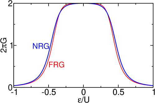
Figure 9: Comaprison of the linear conductance of the SIAM with two metallic leads as a function of $\epsilon$ obtained by approximate FRG and NRG for $U/\Gamma=4\pi$.

For the spin-degenerate SIAM with BCS leads the FRG flow equations for the self-energy and the effective interaction within the low order static approximation read

$$\partial_{\Lambda}\Sigma^{\Lambda} =-\frac{U^{\Lambda}}{\pi}\frac{\epsilon+\Sigma^{\Lambda}}{D^{\Lambda}(i\Lambda)},$$ (68)

$$\partial_{\Lambda}\Sigma_{\Delta}^{\Lambda} =-\frac{U^{\Lambda}}{\pi}\frac{\Sigma_{\Delta}^{\Lambda}-\tilde{\Delta}}{D^{\Lambda}(i\Lambda)},$$ (69)

$$\partial_{\Lambda}U^{\Lambda} =-\frac{2\left(U^{\Lambda}\right)^{2}}{\pi\left[D^{\Lambda}(i\Lambda)\right]^{2}}\left[\left(\epsilon+\Sigma^{\Lambda}\right)^{2}+\left|\tilde{\Delta}-\Sigma_{\Delta}^{\Lambda}\right|\right],$$ (70)

with the initial conditions

$$\Sigma^{\Lambda=\infty}=0,\quad\Sigma_{\Delta}^{\Lambda=\infty}=0,\quad U^{\Lambda=\infty}=U.$$ (71)

Here $D^{\Lambda}$ corresponds to Eq. (35) with $\Sigma$ and $\Sigma_{\Delta}$ replaced by $\Sigma^{\Lambda}$ and $\Sigma_{\Delta}^{\Lambda}$, respectively and $\tilde{\Delta}$ is defined by Eq. (31). The three coupled equations can easily be solved numerically. The Josephson current can be computed at the end of the RG flow inserting $\Sigma^{\Lambda=0}$ and $\Sigma_{\Delta}^{\Lambda=0}$ in Eq. (43). Without loss of generality we now focus on the left-right symmetric case $\Gamma_{L}=\Gamma_{R}=\Gamma$; see Subsect. 2.1. FRG results for the current are compared to highly accurate NRG ones in Fig. 5. It turns out that the truncated FRG captures the quantum phase transition including the jump from $0$- to $\pi$-junction behavior of the current. The exact position of the jump (in the figures as a function of $\phi$) is sensitive to the approximation, however, the overall picture is reproduced quite well by the FRG. It systematically overestimates the current in the doublet phase.

Alternatively the two phases can be identified as follows. In the doublet phase one finds that at a certain $\Lambda_{\rm c}$, $\epsilon+\Sigma^{\Lambda_{\rm c}}=0$. Equation (68) implies that $\Sigma^{\Lambda}=-\epsilon$ for all $\Lambda<\Lambda_{\rm c}$. The off-diagonal component of the self-energy continues to flow and reaches $\Sigma_{\Delta}^{\Lambda=0}=\Gamma\cos(\phi/2)$. Varying the parameters one can identify this behavior and thus determine the phase boundary. The red lines of Fig. 4 were obtained this way. They show excellent agreement with the NRG data even if the interaction $U$ is not small. Inserting $\Sigma^{\Lambda=0}=-\epsilon$ and $\Sigma_{\Delta}^{\Lambda=0}=\Gamma\cos(\phi/2)$ in Eq. (43) yields a result which is independent of $U$ and $\epsilon$. This is an artifact of the approximation and explains why the FRG currents of Fig. 5 do not depend on $U$ in the $\pi$-phase.

The discussion shows that the truncated static FRG provides a easy to use approximate approach which captures the main characteristics of the Anderson-Josephson quantum dot at $\Delta<\infty$ even for fairly large two-particle interactions without suffering from fundamental artifacts such as spurious spin-symmetry breaking. In addition it is flexible and can straightforwardly be extended to more complex dot setups (multi-level, different geometry) to reveal interesting physics. This is exemplified in Sect. 4. However, as for metallic leads a word of warning must be added. It turned out that a systematic extension of the truncation keeping the frequency dependence of the two-particle vertex is not straight forward as briefly discussed in Ref. [33].

3 Comparison to experiments

In this section we compare results of calculations within our minimal model with experimental data. We emphasize that it is not the aim of the present review to give a comprehensive account of the experimental status of the Anderson-Josephson quantum dot; this would require a separate effort. In fact, the presentation of the experiments is reduced to its minimum.

The $T=0$ level crossing quantum phase transition cannot be accessed directly in $T>0$ experiments. Indications of the transition can, however, be found in observables at finite temperatures; see Fig. 6 for the Josephson current. The two most prominent ways of experimentally investigating the physics of the transition induced by the local two-particle interaction are the measurement of the Josephson current and the spectroscopy of the in gap bound states. Here we will focus on the equilibrium current through quantum dots coupled to two conventional s-wave superconducting reservoirs and do not dwell on bound-state spectroscopy; for experiments on the latter, see, e.g., Refs. [77, 78, 79, 80, 81, 82, 83].

The Josephson current was measured in several experiments; recent ones showed indications of the $0$-to-$\pi$ transition.[84, 85, 71, 86, 66, 87, 88] Indium arsenide nanowires[84] and carbon nanotubes[85, 71, 86, 66, 87, 88] were used as quantum dots. The experimental challenge in measuring the true magnitude of the current in SQUID geometries consists in suppressing uncontrolled fluctuations of the superconducting phase difference. This can be achieved using particularly designed on-chip circuits produced by highly advanced nanostructuring techniques. For a short review on the experimental status until 2010, see Ref. [89].

In Ref. [84, 85, 71, 86] the current-voltage [$I(V)$] characteristics of the quantum dot Josephson junction was measured at different gate voltages, i.e., level positions. Applying the extended resistively and capacitively shunted-junction (RCSJ) model[90] from the theory of conventional (structureless) Josephson junctions in an electro-magnetical environment allows one to extract the so-called critical current $J_{\rm c}$ as a function of the gate voltage (but not the full CPR) from the $I(V)$ curves. In this model the CPR is assumed to be purely sinusoidal [compare Eq. (17)] with $J_{\rm c}$ being the amplitude, i.e., the current at $\phi=\pi/2$. A positive $J_{\rm c}$ is thus indicative of the $0$-phase (singlet ground state) and a negative one of the $\pi$-phase (doublet ground state); the gate voltage is the parameter to be used to switch from one to the other. However, due to the assumed form $J(\phi)=J_{\rm c}\sin{\phi}$ this type of analysis is unjustified and leads to meaningless results for $J_{\rm c}$ if higher harmonics contribute to the CPR. Higher harmonics were found to be large in CPRs in which the dot parameters–in particular the gate voltage–are fixed such that the $0$-to-$\pi$-transition is driven by varying the phase difference $\phi$; compare to Figs. 5 and 6. One might thus wonder how this analysis can at all be useful to investigate the level-crossing phase transition. We will comment on this in Subsect. 3.2.

In Refs. [66, 87, 88] the full CPR was measured for different gate voltages. See Ref. [91] for a detailed description of the setup and measurement protocol of how to achieve this.

We already now note that the dot levels investigated in Refs. [71, 86, 66, 87, 88] are in the Kondo regime, however, not very deeply. As the gap $\Delta$ will turn out to be larger than the normal state $T_{\rm K}$ by a factor between 3 and 10 the systems are in the most interesting parameter regime of the competition of Kondo correlations and superconductivity.

3.1 How to extract the parameters

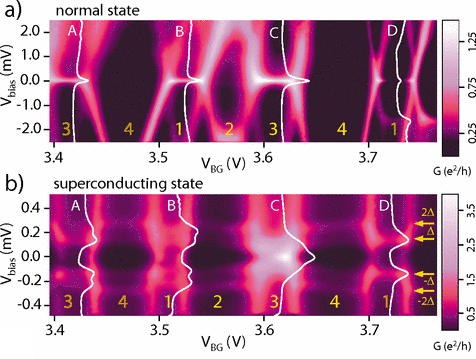
Figure 10: Experimental differential conductance as a function of gate voltage $V_{\rm BG}$ and bias voltage $V_{\rm bias}$ for normal state leads a) and superconducting ones b). Reprinted figures with permission from A. Eichler, R. Deblock, M. Weiss, C. Karrasch, V. Meden, C. Schönenberger, and H. Bouchiat, Phys. Rev. B 79, 161401 (2009). Copyright (2008) by the American Physical Society.

In a first step of the comparison of theory and experiment one has to extract the (model) parameters from the experiment as accurately as possible. The temperature of the system can be estimated with an error of the order of 10% from the nominal temperature of the cryostat and the experience of how to translate this into the electron temperature. Besides $J_{\rm c}$ or the CPR in all experiments considered here the differential conductance $dI/dV$ as a function of bias and gate voltage was measured for superconducting as well as for normal state leads. Superconductivity is destroyed by applying a magnetic (Zeeman) field of strength $h$ known within tight bounds. This also splits the spin-degenerate dot levels and we have to consider the case $\epsilon_{\uparrow}\neq\epsilon_{\downarrow}$ when discussing the situation with normal state leads. Typical $dI/dV$-data taken from Ref. [86] are shown in Fig. 10 a) for the normal state and in b) for the superconducting one. Varying the gate voltage the differential conductance shows partly overlapping repeating structures of comparable shape indicated by the letters A to D. A single one of these structures can be described by the single-level SIAM; for varying gate voltage individual levels move through the transport window. For suppressed superconductivity Fig. 10 a) the bright region at zero bias corresponds to the Kondo ridge of the linear conductance as discussed in Sect. 1.2; see Fig. 1 (b). For the corresponding gate voltages the occupancy is odd [see the yellow numbers in Fig. 10 a)]. In the surrounding dark regions transport is blocked by Coulomb blockade. From this we can conclude that the levels associated to A, B, and C are in the Kondo regime while this does not hold for D. This is supported by the zero bias peaks of the (vertical) white lines which show $dI/dV$ for a fixed gate voltage in the center of the corresponding ridge. The peaks are related to the Kondo peak of the spectral function (see Ref. [12] and references therein). From the edges of each Kondo ridge four lines originate when changing the bias voltage which merge above or below the Kondo ridge center. They are best seen for ridge B and negative bias voltages and are commonly denoted as Coulomb diamonds. From the height of the diamonds the local Coulomb interaction $U$ of the corresponding level A to D can be estimated.[71, 86] For superconducting leads the $dI/dV$-curves show peaks if the bias voltage equals the gap $\Delta$ as can be seen in Fig. 10 b); see the yellow arrows. They originate from the leads BCS density of states and allow to read off $\Delta$. At this stage of the analysis one thus obtained estimates of $U$, $\Delta$, $T$, and $h$ all up to approximately 10% error.

The parameters which are most delicate to determine but strongly affect the Josephson current are $\Gamma$ and $a$. In particular, if the level is in the Kondo regime estimating those from $dI/dV$-curves requires input based on serious many-body theory; simpler theories, e.g., capturing Coulomb blockade only cannot be used. As no fully reliable method to compute finite bias (nonequilibrium) $dI/dV$-curves in the Kondo regime is available it was suggested in Ref. [92] to fit theoretical linear ($V_{\rm bias}=0$) conductance curves as a function of $\epsilon$ [see Fig. 1 (b)] obtained by CTINT QMC (or NRG) to the experimental data to determine $\Gamma$ and $a$. Here the values for $U$, $T$, and $h$ as determined from the procedure described in the last paragraph are used. As discussed in Subsect. 1.2 the width of the Kondo ridge is set by $U/\Gamma$ and allows to determine $\Gamma$, while the height is given by the asymmetry; see Eq. (22). We already now emphasize that both finite temperatures and finite Zeeman fields have to be considered in the calculation as the associated energy scales will turn out to often be comparable in size. Both have the effect to suppress the Kondo ridge in its center (split the ridge), eventually leading to a two peak structure[3]; see Fig. 11 a), left panel. The fitting also allows to determine the so-called gate conversion factor $\alpha$ which relates the change of the level position (unit of energy) to the change of the applied gate voltage (unit of voltage).

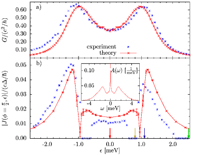
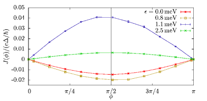
Figure 11: Left panel a): Linear conductance as a function of the level position which is tuned by an applied gate voltage. The blue symbols are experimental data and the red ones theoretical results obtained by fitting $\Gamma$, $a$, and the gate conversion factor $\alpha$ employing CTINT QMC. For more, see the text. Left panel b) main plot: Comparison of experimental and theoretical data for the gate-voltage dependence of the critical current $J_{\rm c}$. Left panel b) inset: The spectral function with normal state leads computed by CTINT QMC. Right panel: Theoretical CPR data for the gate voltages indicated by the arrows in b) (color coded). Reprinted figures with permission from D. Luitz, F. F. Assaad, T. Novotný, C. Karrasch, and V. Meden, Phys. Rev. Lett. 108, 227001 (2012). Copyright (2012) by the American Physical Society.

Figure 11 a), left panel, exemplifies that rather accurate fits can be achieved. The blue symbols show the linear conductance as measured for one of the dot levels (gate voltage regimes) studied in Ref. [71]. For this the procedure described in the second to last paragraph gave $U\approx 3$ meV, $\Delta\approx 0.1$ meV, $T\approx 75$ mK and $h\approx 150$ mT. Given these values the best fit shown as red symbols was obtained for $\Gamma=0.27$ meV, $a=9.3$, and $\alpha=0.011$ V/meV. This implies $U/\Gamma\approx 11.15$ which is sufficiently large for the dot to be in the Kondo regime and to show Kondo physics provided $T$ and $h$ are not too large. To estimate the Kondo scale in the center of the ridge (at exactly odd filling of the dot) we use Eq. (21) and obtain $k_{\rm B}T_{\rm K}\approx 8$ $\mu$eV. This is roughly a factor of $0.03$ smaller than $\Gamma$ (Kondo regime) and of the same order as the energies associated to temperature $k_{\rm B}T\approx 8$ $\mu$eV and the Zeeman field $\mu_{\rm B}h\approx 8.7$ $\mu$eV. Therefore, as already mentioned above, neither the finite temperature nor the field can be neglected when computing observables (e.g. the linear conductance) for suppressed superconductivity. The linear conductance of Fig. 11 a), left panel, shows a Kondo ridge split by temperature and Zeeman field which should not be mistaken with Coulomb blockade peaks which would be located at larger energies $\epsilon\approx\pm U/2\approx\pm 1.5$ meV. That the dot level is in the Kondo regime is also confirmed by the spectral function in the center of the Kondo ridge computed using CTINT QMC for the extracted parameters; see the inset of Fig. 11 b), left panel. It clearly shows a sharp Kondo resonance and Hubbard bands at the expected energies $\omega\approx\pm U/2$. The splitting of the Kondo resonance by the Zeeman field[3] is invisible within the energy resolution of the plot. The spectral function is broadened by the analytic continuation required to obtain real frequency data from CTINT QMC Matsubara ones.[92] While for the dot level considered $k_{\rm B}T_{\rm K}\approx k_{\rm B}T\approx\mu_{\rm B}h$ the gap $\Delta$ is roughly 10 times larger. Kondo correlations can still not be neglected fully and affect the Josephson current.

3.2 The Josephson current

After having determined all parameters it is now possible to compute the CPR by either CTINT QMC or NRG in a parameter-free way and compare to the critical current extracted from the measured current-voltage characteristics of the quantum dot Josephson junction or to the measured full CPR. We start out with the former.

3.2.1 The critical current

The blue symbols in the main plot of Fig. 11 b), left panel, show $\left|J_{\rm c}\right|$ as a function of the level position for the same gate voltage regime as shown in Fig. 11 a), left panel. The data are extracted from the experiment Ref. [71] employing the RCSJ model. Similar results were presented in Ref. [86]. The extraction of the critical current provides only access to its absolute value and not its sign. This is a major drawback (we did not mention above) when it comes to the study of the $0$-to-$\pi$-transition indicated by a sign change of the current. However, solely based on the experimental data one is tempted to conclude that the system is in the $\pi$-(doublet-)phase for $-1$ meV $<\epsilon<1$ meV and in the $0$-(singlet-)phase outside; see Fig. 11 b), left column. As all parameters are known this can be confirmed by calculations within our minimal model which provide access to the sign. The right panel of Fig. 11 shows the computed CPR (by CTINT QMC) for the level positions indicated by the vertical arrows in Fig. 11 b), left column (note the color coding).[92] As expected the current is negative for $-1$ meV $<\epsilon<1$ meV and positive outside this regime. It furthermore shows that even very close to the level-crossing transition at $\epsilon_{\rm c}\approx\pm 1$ meV the CPR is rather sinusoidal (see the light green and blue curves of the right panel of Fig. 11). This is a consequence of $T>0$ and the fairly large left-right asymmetry of the experimental level-lead coupling. Thus the RCSJ model can be employed even close to $\epsilon_{\rm c}\approx\pm 1$ meV and the extracted $\left|J_{\rm c}\right|$ can be used as an indicator of the transition. We emphasize, that these computations are mandatory for the a posteriori justification of the analysis in terms of the RCSJ model. This insight also allows one to use $J(\phi=\pi/2)$ as a measure for the critical current even close to the transition. The red symbols of Fig. 11 b), left column, show the computed $\left|J(\phi=\pi/2)\right|$ in comparison to the experimental $\left|J_{\rm c}\right|$. The error bars indicate the statistical error of the CTINT QMC results. A very satisfying agreement is reached. We reemphasize that the Josephson current is computed without any fitting after the parameters have been extracted in the normal state as described above. It is crucial to use highly accurate methods such as CTINT QMC or NRG to achieve this type of quantitative agreement for dot levels in the (normal-state) Kondo regime as well as $\Delta$ and $T_{\rm K}$ being comparable.

3.2.2 The current-phase relation

Reference [87] reports on the successful measurement of the CPR of a carbon nanotube based quantum dot junction across the entire $0$-to-$\pi$-transition. Additional data were presented in Ref. [88] and details on the setup and measurement protocol are given in Ref. [91]. These works constitute convincing experimental demonstrations of the level-crossing transition controlled by the phase difference $\phi$. The CPR was recorded for different gate voltages, i.e., different positions of the dot level. Figure 12 shows the measured CPRs (green lines) with the amplitude being scaled-up by a unique gate-voltage independent factor (see below). Note that the regime $\phi\in[-\pi,\pi]$ is shown. For the gate voltage of panel (1) the dot is in the $0$-phase with a sinusoidal current of positive amplitude for $\phi\in[0,\pi]$. In (2) the CPR is deformed for $\phi$ close to $\pi$ and no longer a simple harmonic. In (3) the current is negative in this $\phi$ range. For the corresponding level position, varying $\phi$ drives the system through the transition (compare the green curve in Fig. 6, right panel). This trend continues with further decreasing the gate voltage until in panel (6) the dot is in the $\pi$-phase for all $\phi$.

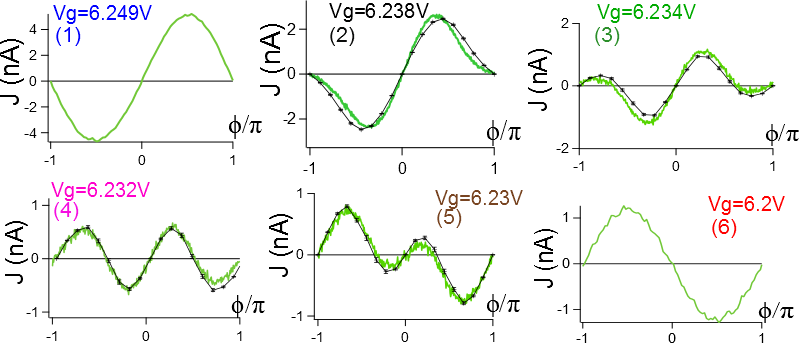
Figure 12: The measured full CPR (green lines) for gate voltages across the phase transition from the $0$- (upper left) to the $\pi$-phase (lower right). For comparison data computed with CTINT QMC are shown as black symbols (the black lines are guides to the eyes). Note that the regime $\varphi\in[-\pi,\pi]$ is shown. For more see the text. Reprinted figure with permission from R. Delagrange, D.J. Luitz, R. Weil, A. Kasumov, V. Meden, H. Bouchiat and R. Deblock, Phys. Rev. B 91, 241401 (2015). Copyright (2015) by the American Physical Society.

Following exactly the same steps as described above the parameters for the dot level considered in Fig. 12 were determined. The values are $U\approx 3.2$ meV, $\Delta\approx 0.17$ meV, $T\approx 150$ mK and $h\approx 1$ T, $\Gamma=0.44$ meV, $a=4$, and $\alpha=0.026$ V/meV all up to an error of the order of 10%. This implies $U/\Gamma=7.27$ and the level is at the boundary of the Kondo regime. To estimate $T_{\rm K}$ we still use Eq. (21) (see the discussion in connection with this equation) which gives $k_{\rm B}T_{\rm K}=48$ $\mu$eV. We thus obtain $\Delta/(k_{\rm B}T_{\rm K})\approx 3.5$.

With the estimated parameters the CPR was computed using CTINT QMC. After shifting the level position by $\delta\epsilon=0.28$ meV and properly adjusting the scaling factor of the amplitude mentioned in the last paragraph the theoretical and experimental data match almost perfectly; compare the green lines and black data points of the central four panels of Fig. 12. It is not surprising that the amplitude of the experimental current has to be scaled up. By construction the measured current is necessarily smaller than the true Josephson current. The QMC calculation predicts a transition region centered around a smaller $\epsilon$ than measured experimentally requiring the shift by $\delta\epsilon=0.28$ meV to superimpose the experimental and theoretical data sets. This shift is currently not understood. Even with this caveat in mind the excellent agreement of the entire line shape of the experimental and theoretical curves for varying level position across the transition region provides a strong indication that (i) the single-level SIAM with BCS leads can be used to describe the experiment and that (ii) the latter shows the finite temperature signatures of the $T=0$ quantum phase transition. Computing the gate voltage dependence of the Fourier coefficients of the experimental and theoretical CPRs by a numerical Fourier transform the comparison was brought to an even higher level in Ref. [87]; see Fig. 4 of this publication.

The quantitative agreement between the measured critical current and CPRs and the ones computed in our model provide a convincing example that the model calculations can directly be applied to measurements. In the minimal model many details (e.g., the details of the leads band structure) are ignored. Focusing on the minimal model, however, allows one to investigate and understand the quantum many-body physics lying at the heart of the level-crossing phase transition in due detail using a combination of well controlled analytical and numerical approaches.

4 More complex dot geometries

We finally exemplify the rich many-body physics which can be found in more complex setups of quantum dots coupled to two superconducting leads. In the first, in addition to being coupled via a single spin-degenerate level, the two BCS leads are coupled directly by a hopping term of the form Eq. (2). In other words, the quantum dot Josephson junction is embedded in a Aharonov-Bohm-like geometry. For small tunnel-coupling via the dot we expect that the Fano effect will play a role. It results from interference of a structureless transport path (via the direct link) and one characterized by a narrow resonance (via the dot). The physics of our second example is driven by the interplay of superconductivity and almost degenerate singlet and triplet two-body states in multi-level dots.

4.1 Reentrance behavior and the Fano effect

The Hamiltonian of the Aharonov-Bohm-like setup is given by the one of our minimal model of Subsect. 2.1 supplemented by the term Eq. (2). For simplicity we here focus on a left-right symmetric setup with $t_{L}=t_{R}$. Following the same steps as in Subsects. 1.1 and 2.1 it is straightforward to show that the expectation value of the current operator is given by the sum of Eqs. (12) and (40) and can thus be written in terms of the lead-dot and lead-lead Green functions

$$J_{L}=\frac{2}{\beta}\sum_{i\omega}\mbox{Im}\,\mbox{Tr}\,\left[t_{L}{\mathcal{G}}_{L,{\rm d}}(i\omega)-t_{\rm d}{\mathcal{G}}_{L,R}(i\omega)\right].$$ (72)

The two terms have a natural interpretation as the dot and direct contribution to the Josephson current. Note however, that the two Green functions are computed in the presence of both the direct link as well as the one across the dot and are thus not identical to the ones derived in Subsects. 1.1 and 2.1, respectively. Employing the equation-of-motion technique the two Green functions can be expressed in terms of the interacting dot Green function and $g_{s}(i\omega)$ Eq. (15). We refrain from reproducing the corresponding expressions which can be found in Ref. [72].

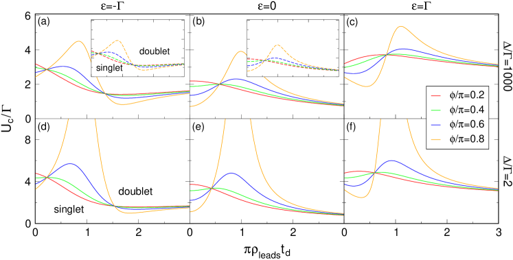
Figure 13: The critical interaction strength $U_{\rm c}$ as a (nonmonotonic) function of the direct coupling $t_{\rm d}$ for different BCS gaps $\Delta$ and impurity energies $\epsilon$, altogether characterizing the singlet-doublet level-crossing phase transition of the Aharonov-Bohm quantum dot Josephson junction. Solid lines where obtained from the FRG approach, dashed lines display the analytic result derived in the limit $\Delta\to\infty$ [see Eq. (75)]. The axis of the insets are scaled the same as the axis of the corresponding main part. Reprinted figure with permission from C. Karrasch and V. Meden, Phys. Rev. B 79, 045110 (2009). Copyright (2009) by the American Physical Society.

To investigate the physics of the Anderson-Josephson-Aharonov-Bohm quantum dot we copy the successful strategy employed above and first study the limit $\Delta\to\infty$. In this limit the noninteracting dot Green function reduces to Eq. (56) with the replacements

$$\epsilon\to\tilde{\epsilon}=\epsilon+\Gamma\frac{\tilde{t}_{\rm d}\cos(\phi)+\tilde{t}_{\rm d}^{3}}{1+2\tilde{t}_{\rm d}^{2}\cos(\phi)+\tilde{t}_{\rm d}^{4}},$$ (73)

$$\Delta_{\rm d}\to\tilde{\Delta}_{\rm d}=\Gamma\cos(\phi/2)\frac{1+{\tilde{t}}_{\rm d}^{2}}{1+2\tilde{t}_{\rm d}^{2}\cos(\phi)+\tilde{t}_{\rm d}^{4}},$$ (74)

with $\tilde{t}_{\rm d}=\pi\rho_{\rm lead}t_{\rm d}$. Fundamental properties of the ground state can again be obtained considering the effective (atomic limit) Hamiltonian Eq. (57) with the same replacements. The condition for a nondegenerate (doubly-degenerate) ground state is thus the same as Eq. (63) with the proper replacements. The equation for the phase boundary separating the two is

$$U^{2}=4\tilde{\epsilon}^{2}+4\tilde{\Delta}_{\rm d}^{2}.$$ (75)

The transition is again a first order level crossing one. However, there is one crucial difference to the $t_{\rm d}=0$ case. Since $\cos(\phi)$ can become negative for $\phi\in[0,\pi]$, the right-hand side of Eq. (75) is not necessarily a monotonic function of the bare parameters $\epsilon/\Gamma$ and $t_{\rm d}/\Gamma$, immediately indicating reentrance behavior and multiple singlet-doublet phase transitions. This is illustrated in the two insets to Fig. 13 which show the critical $U_{\rm c}$ obtained from Eq. (75) for a variety of $\epsilon$ and $\phi$ as a function of $t_{\rm d}$.[72]

This picture of reentrance quantum phase transitions was confirmed for $\Delta<\infty$ by the approximate FRG approach reviewed in Subsect. 2.6. We here refrain from giving the three coupled RG flow equations for the components of the (static) self-energy and the effective two-particle interaction and merely emphasize that they have a structure similar to the ones of Eqs. (68)-(70). They can be found in Ref. [72]. The phase diagram resulting from the numerical solution of these is shown in the main panels of Fig. 13 for a variety of parameter sets. The upper row was computed for $\Delta/\Gamma\gg 1$ and quantitatively confirms the exact $\Delta\to\infty$ results shown in the insets even for sizeable $U/\Gamma$; remind that $U/\Gamma$ is considered as the small parameter in the approximate FRG approach. The behavior remains qualitatively the same for $\Delta/\Gamma$ of order one as shown in the lower row.

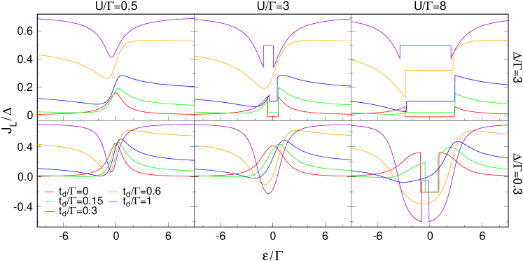
Figure 14: Josephson current $J_{L}$ as a function of the impurity energy $\epsilon$ for constant $\phi=0.5\pi$ and different $t_{d}/\Gamma$ at $T=0$. The results were obtained from the approximate FRG approach. Reprinted figure with permission from C. Karrasch and V. Meden, Phys. Rev. B 79, 045110 (2009). Copyright (2009) by the American Physical Society.

Figure 14 shows the Josephson current as a function of level position for $\phi=\pi/2$ and several sets of the other parameters obtained by FRG. For small interactions (left colum), for which the system is in the singlet state for the considered $t_{\rm d}$ and all $\Delta$ as well as $\epsilon$ the line shape changes from that of a resonance (red line) to the typical S-like Fano line shape (yellow line) to an inverted resonance (violet line) for increasing $t_{\rm d}$. This can similarly be found in the linear-response conductance of the SIAM with metallic leads (see, e.g., Ref. [75] and references therein). For small $\Delta/\Gamma$ this characteristics persists even up to intermediate $U/\Gamma$ (see the central panel of the lower row of Fig. 14). The doublet phase is characterized by the flat parts of $J_{L}(\epsilon)$ [compare to Fig. 11 b), left panel]. The nonmonotonic dependence of the phase boundary on the coupling strength $t_{\rm d}$, see Fig. 13, results in multiple singlet-doublet phase transitions manifesting as the appearance and disappearance of discontinuities of $J_{L}(\epsilon)$ (see in particular the central panel in the upper row of Fig. 14). The behavior of Fig. 14 is generic for arbitrary phase differences $\phi$. For the quantum dot Josephson junction with $t_{\rm d}=0$, the current is positive (negative) in the singlet (doublet) phase. Both facts no longer necessarily hold for $t_{\rm d}>0$ and it would thus be misleading to refer to $0$- and $\pi$-junction behavior. It is intuitive that $J_{L}$ can become positive in the doublet regime due to the additional contribution via the direct link [see Eq. (72)]. Surprisingly one can also observe a negative current in the singlet phase, particularly at small BCS energy gaps $\Delta$ (see the lower row of Fig. 14). We, however, emphasize that this is solely caused by the Coulomb interaction, and the supercurrent at $U=0$ always remains positive. In contrast, Zhang[93] obtained a negative current in the noninteracting limit (for a $U=0$ study, see also Ref. [94]), rendering his results on the current of the Anderson-Josephson-Aharonov-Bohm quantum dot a priori highly questionable. The current of the present systems was also investigated in Ref. [95], however, employing the inappropriate unrestricted mean-field approach; see above.

It would be very interesting to confirm the reentrance phase transition and the Fano line shape of the current for the quantum dot Josephson junction in Aharonov-Bohm geometry in an experiment. For a quantitative comparison between theory and experiment it might then be necessary to apply CTINT QMC or NRG.

4.2 Multi-level dots and singlet-triplet transitions

As a second example of a more complex setup we investigate a geometry with two single-level dots aligned in series and coupled by a hopping $\tau$. The left dot is in addition coupled to a left BCS lead and the right dot to a right BCS lead each by a tunnel coupling as considered before. For definiteness we investigate a fully left-right symmetric setting with $\Gamma_{L}=\Gamma_{R}$, left ($i=1$) and right ($i=2$) dot levels of equal energy as well as equal on-dot and nearest-neighbor two-particle interactions. We emphasize, however, that within the methods used to investigate the system all these restrictions can be relaxed. In the present subsection the Zeeman field splitting the level energies of up and down spins will play an important role. The dot Hamiltonian replacing Eq. (18) reads

$$H_{\rm dot} =\sum_{i=1,2}\left[\left(\bar{\epsilon}+B\right)n_{i,\uparrow}+\left(\bar{\epsilon}-B\right)n_{i,\downarrow}\right]$$

$$+U\sum_{i,\sigma\neq i^{\prime},\sigma^{\prime}}n_{i,\sigma}n_{i^{\prime},\sigma^{\prime}}-\tau\sum_{\sigma}\left(d_{1,\sigma}^{\dagger}d_{2,\sigma}^{\phantom{\dagger}}+\mbox{H.c.}\right),$$ (76)

in self-explaining notation. The gate voltage $\bar{\epsilon}=\epsilon-3U/2$ is shifted such that $\epsilon=0$ corresponds to the point of half filling of the two dots at zero Zeeman field $B=0$. Here we will only discuss the limit $\tau\gg\Gamma$ of two strongly coupled dots. In this case it is sometimes useful to rotate to a bonding and antibonding single-particle basis. For $B=0$ the molecular spin-degenerate levels are energetically well separated. For a discussion of the physics in the opposite limit $\tau/\Gamma\lessapprox 1$, see Ref. [96].

Here we are interested in the following two situations. (i) For vanishing (or small) Zeeman field we expect to find the level-crossing scenario of the single-level Anderson-Josephson dot for both the bonding as well as the antibonding molecular levels if the gate voltage is properly tuned. We will indeed confirm this, which provides further justification for the use of the single-level model when it comes to the comparison to experiments with multi-level dots of sufficiently large level spacings; see Fig. 11. (ii) For a Zeeman field $B\approx\tau$ the single-particle (interaction $U=0$) energies of the bonding spin-up and the anti-bonding spin-down states are almost equal; or rephrased, the smallest two-particle eigenenergies of an isolated dot (with $\Gamma_{L}=0=\Gamma_{R}$ but $U>0$), which are a spin singlet as well as one out of a triplet, are almost degenerate. One might expect that for such Zeeman fields the level crossing scenario is realized as well, with according signatures in the Josephson current. However, this turns out to be only partially true: whereas various characteristics, e.g., the very idea of a level crossing phase transition as well as the corresponding line shapes and parameter dependencies of the current, are just as they are in a single-level case, the magnitude of the supercurrent changes discontinuously at $B=\tau$ in one of the phases. This indicates an additional first order singlet-triplet level-crossing quantum phase transition.

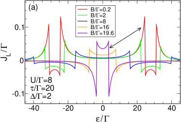
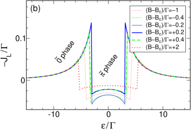
Figure 15: Functional RG results for the $\epsilon$-dependence of the Josephson current $J_{L}$ flowing through the serial quantum dot for generic system parameters $U/\Gamma=8$, $\Delta/\Gamma=2$, $\phi/\pi=0.5$, $\tau/\Gamma=20$, zero temperature, and various Zeeman fields: (a) $B/\Gamma=0.2,2,8,16,19.6$. (b) $B/\Gamma=19,19.6,19.8,20.2,20.4,22$ or $(B-B_{\rm c})/\Gamma=-1,-0.4-0.2,0.2,0.4,2$ with $B_{\rm c}=\tau$. Reprinted figure with permission from C. Karrasch, S. Andergassen, and V. Meden, Phys. Rev. B 84, 134512 (2011). Copyright (2011) by the American Physical Society.

As in the last subsection we will investigate the problem considering $\Delta\to\infty$ (exact solution) and by approximate FRG (for $\Delta<\infty$). As nothing fundamentally new has to be added when setting up the equations of the two approaches we refrain from giving any technical details and focus on the results. The corresponding equations and derivations can be found in Ref. [73].

Figure 15 shows FRG results for the Josephson current as a function of the level position $\epsilon$ obtained for generic system parameters (in particular $\Delta<\infty$) at different $B$. For vanishing or small $B$ [red curve in Fig. 15 (a)] one indeed finds two copies of the single-level behavior located at $\epsilon\approx\pm\epsilon_{0}$ (up to a slight asymmetry around the center of each copy); compare to the red symbols in Fig. 12 for $J_{L}(\epsilon)$. The jump in the current indicates the $0$-to-$\pi$-transition with a negative current in the $\pi$-phase. The inset of Fig. 16, left panel, shows the $\epsilon$-dependence of the current (blue line) and the energy of the lowest lying levels (red lines) for $\Delta\to\infty$, $\epsilon\approx\epsilon_{0}$, and a small Zeeman field. As for the single-dot case we characterize the states by computing the total spin. The ground state is a $\{s=0,m=0\}$ singlet in the $0$-phase or an almost ($B>0$) two-fold generate state $\{s=1/2,m=\pm 1/2\}$ in the $\pi$-phase in strict analogy to the single-level case; compare to Fig. 3 (a).

As $B$ increases, the size of the regions with $J_{L}<0$ increases; see Fig. 15 (a). The transition leading to the jump is a mixture of the transition induced by the two particle interaction, as in Fig. 3 (a), and that induced by the Zeeman field, as in Fig. 3 (b). At $B\approx B_{\rm c}=\tau$, however, a particular behavior can be observed. For this field the single-particle ($U=0$) energies of the anti-bonding spin-up and bonding spin-down states become equal; they cross the Fermi level at $\epsilon=0$. Alternatively this point in parameter space can be characterized as follows: the smallest eigenvalue of $H_{\rm dot}$ (at $U>0$; no leads attached) with two particles, which is the smallest overall one close to $\epsilon=0$, becomes twofold degenerate. The associated spin configuration is either a singlet or (one out of) a triplet. We thus investigate closer whether for $B\approx B_{\rm c}$, $\epsilon\approx 0$ the physics can again be described in a pure (and simple) single-impurity fashion. This is the case for normal leads where finite-$B$ Kondo ridges appear.[97] The Josephson current of the multi-level quantum dot with $B\approx B_{\rm c}$, $\epsilon\approx 0$ indeed resembles the one for $B\approx 0$, $\epsilon\approx\pm\epsilon_{0}$ up to an irrelevant overall sign [see Fig. 15 and compare the curves in (a) which are connected by an arrow]. Characteristically, there are discontinuities associated with a sign change. The regimes of negative and positive current, denoted by $\tilde{0}$ and $\tilde{\pi}$, respectively, show the same dependencies on system parameters as the $0$- and $\pi$-phases of a single impurity. Namely, decreasing $U$, $\epsilon$, $|B-B_{\rm c}|$, or $\pi-\phi$ favors the $\tilde{0}$ regime. Analogously to the line shape of $J_{L}(\epsilon)$, the CPR around $B\approx B_{c}$, $\epsilon\approx 0$ is similar to the single-level case: It is half-sinusoidal (sinusoidal) in the $\tilde{0}$ ($\tilde{\pi}$) regime; compare to Fig. 6.

There is, however, one obvious and interesting difference to the single-level case. For sufficiently large $U/\Gamma$ the current displays another discontinuity at $B=B_{\rm c}$ in addition to the $\tilde{0}$-$\tilde{\pi}$ transition. It is associated with a change in magnitude of $J_{L}$ but not a sign flip as shown in Fig. 15 (b). On both sides of this additional supposedly first-order quantum phase transition, one observes $\tilde{\pi}$ phase behavior as described above. In order to obtain a more thorough understanding of this, we again consider the exactly solvable atomic limit $\Delta=\infty$. The main plot of the left panel of Fig. 16 shows $J_{L}(\epsilon)$ for $B<B_{\rm c}$ and $B>B_{\rm c}$ (blue lines). As for generic $\Delta$ the current is smaller (in fact vanishing for $\Delta\to\infty$) in the latter case, compare to Fig. 15 (b). The main plot of the left panel of Fig. 16 in addition shows the $\epsilon$-dependence of the three lowest lying levels for the case $B>B_{\rm c}$. For such a Zeeman field the ground state in the $\tilde{\pi}$-phase has $s=1$, i.e., is (one out of) a triplet. As shown in the right panel of Fig. 16 (red lines) this changes if $B$ is decreased beyond $B_{\rm c}$ and the ground state becomes a singlet state with $s=0$ in the $\tilde{\pi}$-phase with a discontinuously increased current (blue line). Within the $\tilde{\pi}$-phase one thus finds an additional first order level-crossing phase transition of a singlet and (one out of a) triplet. The same happens for $\Delta<\infty$. It is intuitive that the current is larger in the singlet state as a triplet should prevent Cooper pair tunneling. Using perturbation theory in $\Gamma_{L/R}$ this intuitive picture can be made quantitative as discussed in Ref. [73]. For a similar perturbative analysis which however turned out to be incomplete,[73] see Ref. [98]. We finally note that the above scenario is generic in a broader sense: it is not altered qualitatively if different local- and nearest-neighbor interactions, level detunings or source-drain coupling asymmetries are introduced.

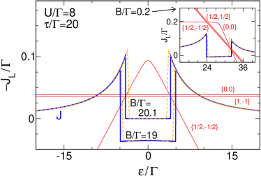
Figure 16: Left panel: Exact results for the zero-temperature Josephson current in the infinite-gap limit (solid blue lines) compared to approximate FRG data obtained at $\Delta/\Gamma=2000$ (dashed orange lines) for three different Zeeman fields. The other parameters are the same as in Fig. 15. Red lines show the three lowest many-particle eigenenergies for $B/\Gamma=20.1$ (main panel) and $B/\Gamma=0.2$ (inset) in arbitrary units. They are labeled by the corresponding spin quantum numbers $\{s,m\}$. Right panel: Atomic-limit ($\Delta\to\infty$) Josephson current (blue line) and the four lowest eigenenergies (red lines; arbitrary units) as a function of the Zeeman field $B$ at $\epsilon=0$. The other parameters are as in Fig. 15. Reprinted figures with permission from C. Karrasch, S. Andergassen, and V. Meden, Phys. Rev. B 84, 134512 (2011). Copyright (2011) by the American Physical Society.

The main plot as well as the inset of the left panel of Fig. 16 show in addition to the exact $\Delta\to\infty$ current (solid blue lines) the one computed by approximate FRG at $\Delta/\Gamma=2000$ (dashed orange lines). The excellent agreement between the two reconfirms that the approximate FRG leads to reliable results even for fairly large $U/\Gamma$ ($=8$ in the figure).

It would be very interesting to experimentally observe the two transitions in a double-dot geometry; the one from the $\tilde{0}$- to the $\tilde{\pi}$-phase and the singlet-triplet transition within the $\tilde{\pi}$-phase. For a quantitative comparison between theory and experiment it might again be necessary to use either NRG or CTINT QMC for the model calculations. In fact, a first step was taken recently. Reference [99] reports on the successful measurement of the critical current in a double-dot structure based on an indium arsenid quantum wire. However, it was only possible to observe the series of $0$-to-$\pi$-transitions at $B=0$; see the red curve in Fig. 15 (a). In this experiment increasing $B$ led to effects which do not seem to be explainable within the simple model and obscure the physics described above. The observed $B$ field dependence appears to originate in the details of the realization of the double-dot.[99] Thus more experimental work is needed.

An extension of the above double-dot model is one in which the coupling $\tau$ is modified such that it includes Rashba spin-orbit coupling. This has interesting effects on the Josephson current as discussed in Refs. [100] and [101]. Note that the spin-orbit coupling might be of relevance in double-dots based on indium arsenid quantum wires (see, e.g., Ref. [99]).

Other aspects of the Josephson current through multi-dot or multi-level systems were studied in Refs. [102, 103, 67, 68, 104, 105, 106].

5 Summary

The aim of the present review is threefold. First, a comprehensive account on the theoretical understanding of the level-crossing phase transition physics of the single-level Anderson-Josephson quantum dot was given. The first order quantum phase transition results from local on-dot correlations. The same are responsible for the Kondo effect. The Kondo effect is not the driving force behind the level-crossing physics as can, e.g., be seen from considering the large gap limit. It is, however, interesting to study the interplay of BCS superconductivity and the Kondo effect. Combining analytical insights from the $U=0$ and the $\Delta\to\infty$ limit as well as highly accurate results obtained by the two numerical approaches NRG and CTINT QMC a deep understanding of the basic physics underlying the transition from a nondegenerate singlet to a doubly-degenerate ground state is gained. This includes an understanding of the finite temperature signatures of the $T=0$ transition. We briefly reviewed the historical development leading to this understanding and evaluated the methods which can be used to obtain reliable results. Our main focus was on the Josephson current as the observable showing the transition. It is characterized by a discontinuous sign change of the current. In the singlet phase the current is positive (for $\phi\in[0,\pi]$) while it is negative in the doublet one, i.e., shows $\pi$-junction behavior. In addition, we reviewed results for the dot spectral function which shows in-gap bound states. As corroborated by our discussion we believe that the physics of the single-level Anderson-Josephson dot is fully understood.

Secondly, we showed that a quantitative agreement between experimental data for the supercurrent and the ones computed with accurate methods applied to the SIAM with BCS leads can be reached. This holds for the gate-voltage dependence of the critical current as well as for the full CPR at varying gate voltage. Details ignored in the model thus do not affect the basics physics captured by the model. For dots which show the Kondo effect at suppressed superconductivity one has to employ methods capturing this to even properly extract the parameters, in particular the hybridizations $\Gamma_{L/R}$. As the experimental current displays the finite temperature signatures of the transition known from the model calculations, which can be carried out at $T=0$ and $T>0$, one can be confident that the experiments indeed show the transition.

Thirdly, we reviewed two examples of how the interaction induced level-crossing physics manifests in more complex dot setups. Experiments on both should be realizable with todays nanostructuring and measurement technology. For an Anderson-Josephson dot embedded in an Aharonov-Bohm-like geometry we discussed reentrance phase transitions showing in the supercurrent. The linear double-dot geometry showed two ground state transitions for a properly tuned Zeeman field. The one known from the single-level case [nondegenerate singlet to (almost) doubly degenerate state] and additionally one in which the ground state turns from a state with spin quantum numbers $\{s=0,m=0\}$ into one with $\{s=1,m=-1\}$. In accordance with the intuition that the former supports Cooper pair transport while the latter inhibits it, the current is larger in the singlet and jumps to a smaller value across this second transition, however, without a sign change. As a general strategy to tackle more complex systems we suggest to use method combination. The parameter space can efficiently be scanned using the computationally cheap FRG. Analytical insights can be obtained in the $\Delta\to\infty$ limit. The parts of the parameter space which show interesting many-body effects can be further investigated with the computationally more demanding NRG or CTINT QMC, in particular, when aiming at a quantitative comparison to experimental data.

References

- [1] Pines D 1961 The many-body problem Frontiers in physics (W. A. Benjamin)
- [2] Grabert H and Devoret M H E 1992 Single Charge Tunneling—Coulomb Blockade Phenomena In Nanostructures Nato Science Series B (Springer US)
- [3] Hewson A C 1997 The Kondo Problem to Heavy Fermions (Cambridge University Press, Cambridge)
- [4] Kondo J 1964 Progress of Theoretical Physics 32 37
- [5] Bulla R, Costi T A and Pruschke T 2008 Rev. Mod. Phys. 80 395
- [6] Tsvelick A and Wiegmann P 1983 Advances in Physics 32 453
- [7] Josephson B 1962 Physics Letters 1 251
- [8] Tinkham M 2004 Introduction to Superconductivity second edition ed (Dover Publications)
- [9] Gubernatis J, Kawashima N and Werner P 2016 Quantum Monte Carlo Methods: Algorithms for Lattice Models (Cambridge University Press)
- [10] Metzner W, Salmhofer M, Honerkamp C, Meden V and Schönhammer K 2012 Rev. Mod. Phys. 84 299
- [11] Martín-Rodero A and Yeyati A L 2011 Advances in Physics 60 899
- [12] Pustilnik M and Glazman L 2004 Journal of Physics: Condensed Matter 16 R513
- [13] Meir Y and Wingreen N S 1992 Phys. Rev. Lett. 68 2512
- [14] Bruus H, Flensberg K and Press O U 2004 Many-Body Quantum Theory in Condensed Matter Physics: An Introduction Oxford Graduate Texts (OUP Oxford)
- [15] Anderson P W 1961 Phys. Rev. 124 41
- [16] Abrikosov A and Gor’kov L 1960 Soviet Physics JETP 12 1243
- [17] Liu S H 1965 Phys. Rev. 137 A1209
- [18] Griffin A 1965 Phys. Rev. Lett. 15 703
- [19] Maki K 1967 Phys. Rev. 153 428
- [20] Salomaa M M 1988 Phys. Rev. B 37 9312
- [21] Yu L 1965 Acta Physica Sinica 21 75
- [22] Shiba H 1968 Progress of Theoretical Physics 40 435
- [23] Rusinov A 1969 JETP Lett. (USSR) (Engl. Transl.) 9
- [24] Soda T, Matsuura T and Nagaoka Y 1967 Progress of Theoretical Physics 38 551
- [25] Müller-Hartmann E 1973 Recent theoretical work on magnetic impurities in superconductors Magnetism ed Suhl H (Academic Press) p 353
- [26] Matsuura T 1977 Progress of Theoretical Physics 57 1823
- [27] Satori K, Shiba H, Sakai O and Shimizu Y 1992 Journal of the Physical Society of Japan 61 3239
- [28] Sakai O, Shimizu Y, Shiba H and Satori K 1993 Journal of the Physical Society of Japan 62 3181
- [29] Kulik I O 1966 Soviet Physics JETP 22 841
- [30] Kulik I O 1966 Soviet Physics JETP 23 529
- [31] Shiba H and Soda T 1969 Progress of Theoretical Physics 41 25
- [32] Bulaevskii L N, Kuzii V V and Sobyianin A A 1977 JETP Lett. 25 290
- [33] Karrasch C 2010 arXiv:1009.3852 PhD thesis (RWTH Aachen University)
- [34] Žonda M, Pokorný V, Janiš V and Novotný T 2016 Phys. Rev. B 93 024523
- [35] Karrasch C, Oguri A and Meden V 2008 Phys. Rev. B 77 024517
- [36] Kadlecová A, Žonda M and Novotný T 2017 Phys. Rev. B 95 195114
- [37] Yoshioka T and Ohashi Y 2000 Journal of the Physical Society of Japan 69 1812
- [38] Rozhkov A V and Arovas D P 2000 Phys. Rev. B 62 6687
- [39] Tanaka Y, Oguri A and Hewson A C 2007 New Journal of Physics 9 115
- [40] Choi M S, Lee M, Kang K and Belzig W 2004 Phys. Rev. B 70 020502
- [41] Oguri A, Tanaka Y and C Hewson A 2004 Journal of the Physical Society of Japan 73 2494
- [42] Siano F and Egger R 2004 Phys. Rev. Lett. 93 047002
- [43] Luitz D J and Assaad F F 2010 Phys. Rev. B 81 024509
- [44] Bauer J, Oguri A and Hewson A C 2007 Journal of Physics: Condensed Matter 19 486211
- [45] Hecht T, Weichselbaum A, von Delft J and Bulla R 2008 Journal of Physics: Condensed Matter 20 275213
- [46] Jarrell M, Sivia D S and Patton B 1990 Phys. Rev. B 42 4804
- [47] Pokorný V and Žonda M 2018 Physica B: Condensed Matter 536 488
- [48] Kadlecová A, Žonda M, Pokorný V and Novotný T 2018 arXiv:1807.07017
- [49] Glazman L I and Matveev K A 1989 JETP Letters 49 659
- [50] Spivak B I and Kivelson S A 1991 Phys. Rev. B 43 3740
- [51] Novotný T, Rossini A and Flensberg K 2005 Phys. Rev. B 72 224502
- [52] Governale M, Pala M G and König J 2008 Phys. Rev. B 77 134513
- [53] Zuckermann M J 1965 Phys. Rev. 140 A899
- [54] Takanaka K and Takano F 1966 Progress of Theoretical Physics 36 1080
- [55] Shiba H 1973 Progress of Theoretical Physics 50 50
- [56] Rozhkov A V and Arovas D P 1999 Phys. Rev. Lett. 82 2788
- [57] Žonda M, Pokorný V, Janiš V and Novotný T 2015 Scientific Reports 5 8821
- [58] Alastalo A T, Joynt R J and Salomaa M M 1998 Journal of Physics: Condensed Matter 10 L63
- [59] Vecino E, Martín-Rodero A and Yeyati A L 2003 Phys. Rev. B 68 035105
- [60] Bickers N E 1987 Rev. Mod. Phys. 59 845
- [61] Ishizaka S, Sone J and Ando T 1995 Phys. Rev. B 52 8358
- [62] Clerk A A and Ambegaokar V 2000 Phys. Rev. B 61 9109
- [63] Sellier G, Kopp T, Kroha J and Barash Y S 2005 Phys. Rev. B 72 174502
- [64] Meng T, Florens S and Simon P 2009 Phys. Rev. B 79 224521
- [65] Wentzell N, Florens S, Meng T, Meden V and Andergassen S 2016 Phys. Rev. B 94 085151
- [66] Maurand R, Meng T, Bonet E, Florens S, Marty L and Wernsdorfer W 2012 Phys. Rev. X 2 011009
- [67] Bergeret F S, Yeyati A L and Martín-Rodero A 2006 Phys. Rev. B 74 132505
- [68] Bergeret F S, Yeyati A L and Martín-Rodero A 2007 Phys. Rev. B 76 174510
- [69] Allub R and Proetto C R 2015 Phys. Rev. B 91 045442
- [70] Kiršanskas G, Goldstein M, Flensberg K, Glazman L I and Paaske J 2015 Phys. Rev. B 92 235422
- [71] Jørgensen H I, Novotný T, Grove-Rasmussen K, Flensberg K and Lindelof P E 2007 Nano Letters 7 2441
- [72] Karrasch C and Meden V 2009 Phys. Rev. B 79 045110
- [73] Karrasch C, Andergassen S and Meden V 2011 Phys. Rev. B 84 134512
- [74] Kopietz P, Bartosch L and Schütz F 2010 Introduction to the Functional Renormalization Group Lecture Notes in Physics (Springer)
- [75] Karrasch C, Enss T and Meden V 2006 Phys. Rev. B 73 235337
- [76] Karrasch C, Hedden R, Peters R, Pruschke T, Schönhammer K and Meden V 2008 Journal of Physics: Condensed Matter 20 345205
- [77] Pillet J D, Quay C H L, Morfin P, Bena C, Yeyati A L and Joyez P 2010 Nat. Phys. 6 965
- [78] Deacon R S, Tanaka Y, Oiwa A, Sakano R, Yoshida K, Shibata K, Hirakawa K and Tarucha S 2010 Phys. Rev. Lett. 104 076805
- [79] Franke K J, Schulze G and Pascual J I 2011 Science 332 940
- [80] Pillet J D, Joyez P, Žitko R and Goffman M F 2013 Phys. Rev. B 88 045101
- [81] Chang W, Manucharyan V E, Jespersen T S, Nygård J and Marcus C M 2013 Phys. Rev. Lett. 110 217005
- [82] Kim B K, Ahn Y H, Kim J J, Choi M S, Bae M H, Kang K, Lim J S, López R and Kim N 2013 Phys. Rev. Lett. 110 076803
- [83] Grove-Rasmussen K, Steffensen G, Jellinggaard A, Madsen M H, Žitko R, Paaske J and Nygård J 2018 Nature Commun. 9 2376
- [84] van Dam J A, Nazarov Y V, Bakkers E P A M, De Franceschi S and P K L 2006 Nature 442 667
- [85] Cleuziou J P, Wernsdorfer W, Bouchiat V, Ondarçuhu T and Monthioux M 2006 Nature Nanotech. 1 53
- [86] Eichler A, Deblock R, Weiss M, Karrasch C, Meden V, Schönenberger C and Bouchiat H 2009 Phys. Rev. B 79 161407
- [87] Delagrange R, Luitz D J, Weil R, Kasumov A, Meden V, Bouchiat H and Deblock R 2015 Phys. Rev. B 91 241401
- [88] Delagrange R, Weil R, Kasumov A, Ferrier M, Bouchiat H and Deblock R 2016 Phys. Rev. B 93 195437
- [89] De Franceschi S, Kouwenhoven L, Schönenberger C and Wernsdorfer W 2010 Nature Nanotech. 5 703
- [90] Ambegaokar V and Halperin B I 1969 Phys. Rev. Lett. 22 1364
- [91] Basset J, Delagrange R, Weil R, Kasumov A, Bouchiat H and Deblock R 2014 Journal of Applied Physics 116 024311
- [92] Luitz D J, Assaad F F, Novotný T, Karrasch C and Meden V 2012 Phys. Rev. Lett. 108 227001
- [93] Zhang Z Y 2005 Journal of Physics: Condensed Matter 17 4637
- [94] Cheng S G, Xing Y X, Xie X C and Sun Q F 2009 The European Physical Journal B 67 551
- [95] Osawa K, Kurihara S and Yokoshi N 2008 Phys. Rev. B 78 224508
- [96] Žitko R, Lee M, López R, Aguado R and Choi M S 2010 Phys. Rev. Lett. 105 116803
- [97] Grap S, Andergassen S, Paaske J and Meden V 2011 Phys. Rev. B 83 115115
- [98] Lee M, Jonckheere T and Martin T 2010 Phys. Rev. B 81 155114
- [99] Estrada Saldaña J C, Vekris V, Steffensen G, Žitko R, Krogstrup P, Paaske J, Grove-Rasmussen K and Nygård J 2018 arXiv:1808.05837
- [100] Droste S, Andergassen S and Splettstoesser J 2012 Journal of Physics: Condensed Matter 24 415301
- [101] Brunetti A, Zazunov A, Kundu A and Egger R 2013 Phys. Rev. B 88 144515
- [102] Choi M S, Bruder C and Loss D 2000 Phys. Rev. B 62 13569
- [103] Zhu Y, Sun Q f and Lin T h 2002 Phys. Rev. B 66 085306
- [104] López R, Choi M S and Aguado R 2007 Phys. Rev. B 75 045132
- [105] Zazunov A, Yeyati A L and Egger R 2010 Phys. Rev. B 81 012502
- [106] Yi G Y, Wang X Q, Gong W J, Wu H N and Chen X H 2016 Physics Letters A 380 1385