Ergodic Capacity of Triple-Hop All-Optical Amplify-and-Forward Relaying over Free-Space Optical Channels

Abstract

In this paper, we propose a comprehensive research over triple hop all-optical relaying free-space optical (FSO) systems in the presence of all main noise sources including background, thermal and amplified spontaneous emission (ASE) noise and by considering the effect of the optical degree-of-freedom (DoF). Using full CSI relaying, we derive the exact expressions for the noise variance at the destination. Then, in order to simplify the analytical expressions of full CSI relaying, we also propose and investigate the validity of different approximations over noise variance at the destination. Finally, we evaluate the the performance of considered triple-hop all-optical relaying FSO system in term of ergodic capacity.

I Introduction

The rapidly increasing need of very high data rate communications made free space optical (FSO) communication very popular during the past few years. FSO communication offers a great potential due to the ease of deployment, unregulated frequency band and the enormous available bandwidth [1]. FSO communication has observed great scientific developments and engineering improvements that make it usable for various commercial, industrial, military, environmental, and sensor network applications [2, 3]. However, atmospheric turbulence-induced fading, geometrical spread and channel loss, which are distance-dependent, significantly decrease the FSO link performance [4, 5, 6]. To overcome this limitation, relaying techniques to divide a long link into multiple short links, has been advocated for FSO transceivers as a mean to cover large distances and improve the performance of FSO systems [7].

Research studies on relay-assisted FSO systems was initially focused on electrical relaying where electrical-optical and optical-electrical conversions was performed at relays [8, 9, 10]. However, it is well known that the efficiency of electrical relaying is limited due to the requirement of high-speed electrons and optoelectronic hardware. Moreover, by developing tracking systems using acousto-optic devices that especially applicable to the fast moving unmanned aerial vehicles (UAVs) for compensating the pointing losses, UAV-based FSO communication systems are employed for high data transmission between moving UAVs [11]. However, due to the power, size and weight constraints of UAV systems, in practice, all-optical relaying is preferred to relying optical signals between UAVs [12]. To avoid the inherent complexities associated with electrical-optical and optical-electrical conversions in electrical relays, a new setup of relay-assisted FSO system referred to as all-optical relaying was recently proposed in the context of FSO communication where all processing are done in the optical domain [13, 14, 15, 16, 17, 18, 19, 20, 21, 22, 23]. In particular, in [19], optical amplify and optical regenerate techniques were developed and bit error rate (BER) performance was investigated by using Monte-Carlo (M-C) simulations. However, the latter work does not consider the effect of amplified spontaneous emission (ASE) noise. In [20], the outage probability for a dual-hop FSO relay system was investigated in which ASE noise of optical amplifier was considered. However, in [20], the authors have not considered the effect of the optical degree-of-freedom (DoF). In [21] and [22], the outage probability of a dual-hop and parallel all-optical relaying was studied in which the effects of both ASE noise and optical DoF was considered. However, performance analysis performed in [21, 22], is based on the assumption that the effects of the background and thermal noises are negligible compared to the effect of the ASE noise. Recently, in [23] a comprehensive signal model for a more precise analysis of dual-hop all-optical relaying FSO systems is studied in the presence of all main noise sources. In [23] the authors shown that due to the presence of background and ASE noise, the optimal location of the relay node is not placed at half distance of transceiver.

In this paper, we extend the results of [23] and investigate the performance of triple-hop all-optical FSO system relaying. Particularly, using full CSI relaying, we derive the exact expressions for the noise variance at the destination in the presence of all main source noises including background, thermal and ASE noise by taking into account the presence of DoF. Then, in order to simplify the analytical expressions of full CSI relaying, we also propose and investigate the validity of different approximations over noise variance at the destination. The motivation of this paper is answering to this question: what is the relationship between relay locations and noise sources. For this aim numerical results are plotted in term of ergodic capacity versus different values of source-to-relay, relay-to-relay and relay-to-destination. Simulation results revealed that the optimal relay locations strongly depend on noise sources.

The rest of this paper is organized as follows. In Section II, we describe the triple-hop FSO system model along with our main assumptions. In this Section, we derive the noise variance at the destination. we propose some approximations over noise variance at the destination. In Section III, we study the performance of considered system in term of ergodic capacity throw numerical results. Finally in Section IV, we draw our conclusions.

II System Model

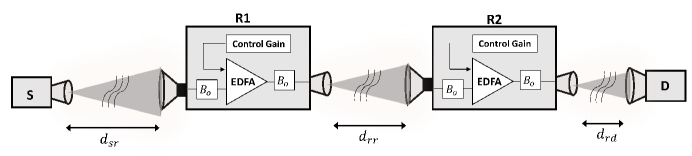
Figure 1: All-optical triple-hop FSO system model.

In this paper, we consider a relay-assisted intensity modulation-direct detection (IM-DD) FSO system, where the information at the source is transmitted to the destination through two all-optical AF relay network, i.e., the process of reception, amplification and retransmission are done in the optical domain. The source-to-destination (SD) link length is $d_{sd}=d_{sr}+d_{rr}+d_{rd}$, where $d_{sr}$, $d_{rr}$ and $d_{rd}$ are source-to-relay (SR), relay-to-relay (RR) and relay-to-destination (RD) link length. As depicted in Fig. 1, the considered system model includes the following main parts: transmitter, turbulence channel, all-optical relays and receiver. In the sequel, we analyze these four parts with more details to obtain the mathematical models for the signals and noises at the destination in the context of all-optical relaying system.

II-1 Transmitter

It is assumed that the transmitter is equipped with a laser diode operating at wavelength $\lambda=$ 1550 nm. Notice that the 1550 nm band is compatible with erbium-doped fiber amplifier (EDFA) technology, which is useful for long range FSO links to improve their performance [27]. The mean photon counts of the transmitted pulses is $m_{t}=P_{t}T_{s}/h_{p}\nu$, where $P_{t}$, $T_{s}$, $\nu$ and $h_{p}$ are the transmitted power, chip duration, optical frequency and Plank’s constant, respectively. For convenience, we use the notations $m_{s}$, $m_{r1}$ and $m_{r2}$ to denote the mean of transmitted photon counts at source, first and second relay, respectively.

II-2 FSO Channel

We assume that the transmitted power is attenuated by two factors: the path loss $h_{l}$ and the atmospheric turbulence $h_{a}$. Hence, the channel gain $h$ can be formulated as $h=h_{l}h_{a}$. The path loss $h_{l}$ is a function of the optical wavelength $\lambda$, divergence angle $\theta_{\rm div}$ and link length $d$, and can be expressed as [28]

$$h_{l}=\frac{A_{a}}{\left(\theta_{\rm div}d/2\right)^{2}}h_{l}^{\prime}~{},$$ (1)

where $A_{a}$ is the receiver aperture area and $h_{l}^{\prime}$ is the atmospheric attenuation which is modeled by the exponential Beers-Lambert Law as $h_{l}^{\prime}=\exp\left(-d\xi\right)$ and $\xi$ is the scattering coefficient [28]. For clear and foggy weather conditions, the scattering coefficient is a function of the visibility $\mathcal{V}$, and can be written as [28]

$$\xi=\frac{3.91}{\mathcal{V}}\left(\frac{\lambda}{550}\right)^{-q},$$ (2)

where $q$ is equal to 1.6, 1.3 and 0.585$\mathcal{V}^{1/3}$ for $\mathcal{V}>50$ Km, 50 Km$>\mathcal{V}>6$ Km and $\mathcal{V}<6$ Km, respectively.

We model the turbulence-induced fading $h_{a}$ by a log-normal distribution, i.e., $\ln\mathcal{N}(h_{a};\mu_{l,h_{a}},\sigma_{l,h_{a}}^{2})$, which is emerged as a useful model for a weak atmospheric turbulence regime [29]. The probability density function (PDF) of the log-normal model is given by

$$f_{h_{a}}(h_{a})=\frac{1}{h_{a}\sigma_{l,h_{a}}\sqrt{2\pi}}\exp\left(-\frac{\left(\ln h_{a}-\mu_{l,h_{a}}\right)^{2}}{2\sigma^{2}_{l,h_{a}}}\right).$$ (3)

To ensure that fading does not attenuate or amplify the average power, we normalize the fading coefficients such that $\mu_{h_{a}}=1$. Doing so requires the choice of $\mu_{l,h_{a}}=-\sigma^{2}_{l,h_{a}}/2$. Notice that $\sigma^{2}_{l,h_{a}}\simeq\sigma^{2}_{R}/4$ where $\sigma^{2}_{R}$ is the Rytov variance and can be measured directly from atmospheric parameters as [1]

$$\sigma^{2}_{R}=1.23C_{n}^{2}\kappa^{7/6}d^{11/6},$$ (4)

where $\kappa=2\pi/\lambda$ and $C_{n}^{2}$ is the refractive index structure constant. In this paper, we assume that the transceivers are perfectly aligned.

Since, the channel gain is modeled as $h=h_{l}h_{a}$, hence, $h$ is distributed according to the log-normal distribution $\ln\mathcal{N}(h;\mu_{l,h},\sigma_{l,h}^{2})$ where $\mu_{l,h}=-\sigma^{2}_{R}/8+\ln(h_{l})$ and $\sigma_{l,h}^{2}=\sigma^{2}_{R}/4$. For convenience, we use the notations $h_{sr}$, $h_{rr}$ and $h_{rd}$ to denote the SR, RR and RD channel gains, respectively.

II-3 EDFA-Based Relays

At the relay nodes, the incoming optical light is guided into the optical fiber by a converging lens. However, in addition to the desired optical signal, the undesired background light due to the scattered sunlight is also collected by the receiver. The collected optical light is then amplified by an EDFA to compensate the channel loss. An EDFA is characterized by the noise factor $K=n_{sp}(G-1)$, the number of spontaneous mode $D$, and gain $G$ where, $n_{sp}$ is the amplifier spontaneous emission factor. Assuming that the ASE noise is modeled by an additive noise (similar to the background noise), the photon count $n$, at the output of first relay is Laguerre distributed as [30, 27]

$$f_{n,r_{1}}(n)=Lag\left\{n,G_{1}m_{s}h_{sr},G_{1}(m_{br_{1}}+n_{sp}),D\right\},$$ (5)

where $m_{br_{1}}=P_{br_{1}}T_{s}/h_{p}\nu$ and $P_{br_{1}}$ is the filtered background power at first relay. The distribution of Laguerre (also known as the non-central negative-binomial) is given in [27, Eq. (5)]. Moreover, the mean and the variance of $Lag\{n,a,b,D\}$ are respectively derived in [27, Eq. (7)] as

$$m_{{\rm Lag}}(a,b,D)=a+Db,$$

$${\it Var}_{{\rm Lag}} (a,b,D)=a+D(b+b^{2})+2ab.$$ (6)

Similar to the approach followed by most of existing work in the context of dual-hop FSO communications [20, 22, 21], in this paper, full CSI relaying (variable gain) is considered. Note that, for FSO channels, CSI can be easily obtained over a sequence of received bits [24, 25]. In full CSI relaying, the instantaneous CSI of the SR and RR links are assumed to be known at the relays. First and second relays set the amplifier gains based on the instantaneous fading of the SR and RR links $h_{sr}$ and $h_{rr}$, respectively, in such a way that the relay output powers $P_{r_{1}}$ and $P_{r_{2}}$, are kept constant at all time-slots. Due to the high gain of EDFAs (i.e., $G\gg 1$), in this paper, we approximate the noise factor as $K\simeq n_{sp}G$. The amplifier gains of both first and second relays are calculated as [21]

$$G_{1}= \frac{m_{r_{1}}}{m_{s}h_{sr}+D(m_{br_{1}}+n_{sp})},$$ (7)

$$G_{2}= \frac{m_{r_{2}}}{m_{r_{1}}h_{rr}+D(m_{br_{2}}+n_{sp})},$$ (8)

where $m_{r_{1}}=P_{r_{1}}T_{s}/h_{p}\nu$ and $m_{r_{2}}=P_{r_{2}}T_{s}/h_{p}\nu$ are the average transmitted photons by first and second relays, respectively. According to (5), the photon count $n$, at the output of second relay is distributed as

$$f_{n,r_{2}}(n)=Lag\Big{\{} n,G_{1}G_{2}m_{s}h_{sr}h_{rr},G_{1}G_{2}(m_{br_{1}}+n_{sp})h_{rr}$$

$$+G_{2}(m_{br_{2}}+n_{sp}),D\Big{\}},$$ (9)

where $m_{br_{2}}=P_{br_{2}}T_{s}/h_{p}\nu$ and $P_{br_{2}}$ is the filtered background power at second relay.

II-4 Signal Model at Destination

The amplified optical signal is forwarded to the destination via a transmitting lens. At destination, the received optical signal, including the background radiation, is collected and focused on the surface of a photo-detector. Based on (II-3), the photon count $n$, at the input of photo-detector has also a Laguerre distribution as

$$f_{n,d}(n)= Lag\Big{\{}n,G_{1}G_{2}m_{s}h_{sr}h_{rr}h_{rd},G_{1}G_{2}(m_{br_{1}}+n_{sp})$$

$$\times h_{rr}h_{rd}+G_{2}(m_{br_{2}}+n_{sp})h_{rd}+m_{bd},D\Big{\}},$$ (10)

where $m_{bd}=P_{bd}T_{s}/h_{p}\nu$ and $P_{bd}$ is the filtered background power at destination. At the destination, the collected optical signal is converted to an electrical one by a photo-detector (PD). The Laguerre distribution has the property that it preserves its form after photo-detection and $Lag(n,a,b,D)$ is converted to $Lag\{n,\eta a,\eta b,D\}$ by a photo-detector with quantum efficiency $\eta$ [27]. Hence, the photon count distribution at destination, without considering the effect of thermal noise, is derived as

$$f^{\prime}_{n,d}(n)= Lag\Big{\{}n,\eta G_{1}G_{2}m_{s}h_{sr}h_{rr}h_{rd},\eta G_{1}G_{2}(m_{br_{1}}+n_{sp})$$

$$\times h_{rr}h_{rd}+\eta G_{2}(m_{br_{2}}+n_{sp})h_{rd}+\eta m_{bd},D\Big{\}}.$$ (11)

By substituting (II-4) in (II-3) and without considering the effect of thermal noise after photo-detection process, the mean and variance of photon count at destination are respectively derived as

$$m^{\prime}_{d} =\eta G_{1}G_{2}m_{s}h_{sr}h_{rr}h_{rd}$$

$$~{}~{}~{}+\eta DG_{1}G_{2}(m_{br_{1}}+n_{sp})h_{rr}h_{rd}$$

$$~{}~{}~{}+\eta DG_{2}(m_{br_{2}}+n_{sp})h_{rd}+\eta Dm_{bd},$$ (12)

and

$$\sigma^{\prime 2}_{d}= \eta G_{1}G_{2}m_{s}\big{(}1+2\eta m_{bd}\big{)}h_{sr}h_{rr}h_{rd}$$

$$+\eta DG_{1}G_{2}(m_{br_{1}}+n_{sp})\big{(}1+2\eta m_{bd}\big{)}h_{rr}h_{rd}$$

$$+\eta DG_{2}(m_{br_{2}}+n_{sp})\big{(}1+2\eta m_{bd}\big{)}h_{rd}$$

$$+D\big{(}\eta G_{1}G_{2}(m_{br_{1}}+n_{sp})\big{)}^{2}h_{rr}^{2}h_{rd}^{2}$$

$$+D\big{(}\eta G_{2}(m_{br_{2}}+n_{sp})\big{)}^{2}h_{rd}^{2}$$

$$+2\eta^{2}G_{1}G_{2}^{2}(m_{br_{1}}+n_{sp})(m_{br_{2}}+n_{sp})h_{rr}h_{rd}^{2}$$

$$+2\eta^{2}G_{1}^{2}G_{2}^{2}m_{s}(m_{br_{1}}+n_{sp})h_{sr}h_{rr}^{2}h_{rd}^{2}$$

$$+2\eta^{2}G_{1}G_{2}^{2}m_{s}(m_{br_{2}}+n_{sp})h_{sr}h_{rr}h_{rd}^{2}$$

$$+\eta D\big{(}m_{bd}+m_{bd}^{2}\big{)}.$$ (13)

Because of the large number of photons after optical amplification, the mean and the variance of the received photon count at the destination can be approximated closely by a Gaussian [27]. Moreover, the thermal noise is generated independently from the received optical signal and has a zero-mean Gaussian distribution with variance due to the resistive element

$$\sigma^{2}_{th}=\frac{2K_{B}T_{R}T_{s}}{R_{L}e^{2}},$$ (14)

where $K_{B}$ is the Boltzmann constant, $T_{R}$ and $R_{L}$ are the receiver’s equivalent temperature and load, and $e$ denotes the electron charge. While dark current noise can practically be neglected, the photo-electron count at the destination can accurately be modeled by a Gaussian distribution with mean $m_{d}=m^{\prime}_{d}$ and variance

$$\sigma_{d}^{2}=\sigma^{\prime 2}_{d}+\sigma_{th}^{2}.$$ (15)

Finally, the electrical SNR at destination is expressed as

$$\gamma=\left(\eta G_{1}G_{2}m_{s}h_{sr}h_{rr}h_{rd}\right)^{2}/\sigma_{d}^{2}.$$ (16)

As we observe from (II-4) and (15), the variance of noise at the destination is very complex. In order to simplify, in the sequel, we propose two approximations over noise variance and then, in the Section III we investigate the accuracy of these approximations. First, we consider the practical case where the amount of background power is low. At this condition, the noise variance at the destination can be approximated as

$$\sigma^{2}_{d}\simeq ~{}2\eta^{2}G_{1}^{2}G_{2}^{2}m_{s}(m_{br_{1}}+n_{sp})h_{sr}h_{rr}^{2}h_{rd}^{2}$$

$$+2\eta^{2}G_{1}G_{2}^{2}m_{s}(m_{br_{2}}+n_{sp})h_{sr}h_{rr}h_{rd}^{2}+\sigma_{th}^{2}.$$ (17)

To study the effect thermal noise has on the performance of the considered dual hop FSO system, we assume that the SNR at the destination is limited by thermal noise. According this assumption, noise variance at the destination is simplified as

$$\sigma_{d}^{2}\simeq\sigma^{2}_{th}.$$ (18)

III Numerical Results and Discussions

We now present numerical and analytical results to evaluate the performance of the considered triple-hop FSO system over log-normal turbulence channel. Different system parameters used throughout performance evaluation are provided in Table I. To facilitate numerical analysis, we consider a similar condition for SR, RR and RD links, i.e., parameters such as visibility $\mathcal{V}$, refractive index structure constant $C_{n}^{2}$, background power $P_{br1}=P_{br1}=P_{bd}=P_{b}$, and divergence angle $\theta_{div}$, are set equal in both channels.

In this paper, we analyze the performance of considered system in term of ergodic or average capacity. As we observe from (16), electrical SNR at the destination is a function of $h_{sr}$, $h_{rr}$ and $h_{rd}$. Hence, for considered system, ergodic capacity can be obtained as

$$\mathcal{C}_{\rm erg}= \int_{0}^{\infty}\!\!\int_{0}^{\infty}\!\!\int_{0}^{\infty}\log\Big{(}1+\gamma(h_{sr},h_{rr},h_{rd})\Big{)}dh_{sr}dh_{rr}dh_{rd}.$$ (19)

TABLE I: System Parameters Used for Simulations

Description	Parameter	Setting
Wavelength	$\lambda$	$1550$ nm
Source-to-destination length	$d_{sd}$	5 km
Visibility	$\mathcal{V}$	1.5 km
Refractive index	$C_{n}^{2}$	$10^{-15}$
Aperture area	$A_{a}$	$\pi(0.1)^{2}$
Divergence angle	$\theta_{div}$	$1$ mrad
Plank's Constant	$h_{p}$	$6.6\times 10^{-34}$
Boltzmann's Constant	$K_{B}$	$1.38\times 10^{-23}$
Receiver Load	$R_{L}$	$100~{}\Omega$
Receiver Temperature	$T_{R}$	$300\degree~{}K$
Transfer Rate	$R_{s}$	2 Gbit/s
Symbol Duration	$T_{s}$	$1/R_{s}$ s
Spontaneous emission parameter	$n_{s}$	1
DoF	$D$	100
Quantum efficiency	$\eta$	0.8
Average transmit power of source	$P_{s}$	5 dBm W
Average transmit power of relays	$P_{r_{1}}\&P_{r_{2}}$	5 dBm W

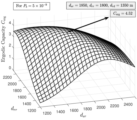
Figure 2: Average capacity of FSO relaying system versus SR link length $d_{sr}$, and RR link length $d_{rr}$ for a fixed SD link length $d_{sd}=5$ km and $P_{b}=5\times 10^{-9}$.

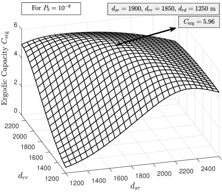
Figure 3: Average capacity of FSO relaying system versus SR link length $d_{sr}$, and RR link length $d_{rr}$ for a fixed SD link length $d_{sd}=5$ km and $P_{b}=10^{-9}$.

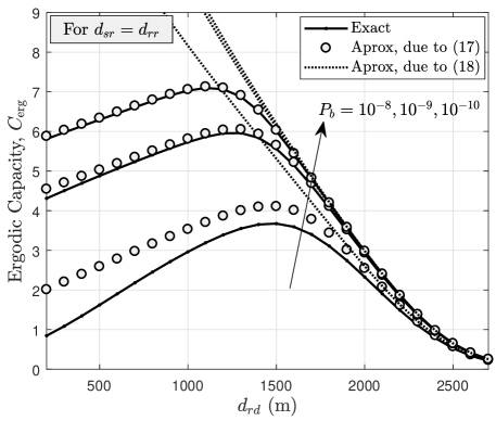
Figure 4: Average capacity of FSO relaying system versus RD link length $d_{rd}$ for a fixed SD link length $d_{sd}=5$ km and different values of $P_{b}$.

To demonstrate the effects of optimum relay location on the performance of the considered triple-hop FSO system, in Figs. 2 and 3, we have plotted the ergodic capacity versus SR link length $d_{sr}$, and RR link length $d_{rr}$ for a fixed SD link length $d_{sd}=5$ km. Figure 2 is depicted for $P_{b}=5\times 10^{-9}$ and Fig. 3 is depicted for $P_{b}=10^{-9}$. There are three important observations which can be drawn from these figures. First, the performance strongly depends on the relay locations and as we observe, by changing relay locations the ergodic capacity changes, significantly. Second, the optimum location of relays (the location with higher ergodic capacity) depends on the background noise level. For instance, for $P_{b}=5\times 10^{-9}$, the optimum location of relays are achieved at $d_{sr}=1850$, $d_{rr}=1800$ and $d_{rd}=1350$ m and for $P_{b}=10^{-9}$, the optimum location of relays are achieved at $d_{sr}=1900$, $d_{rr}=1850$ and $d_{rd}=1250$ m. Third, at the optimum location of relays, SR link length is approximately equal to RR link length and they are bigger than that RD link length.

Now we want to investigate the validity of approximations on (II-4) which are characterized by (II-4) and (18). To this aim, in Fig. 4, we have plotted the ergodic capacity versus $d_{rd}$ for different values of $P_{b}$ where $d_{sr}=d_{rr}$. In addition to the conclusions drawn form the simulation results proposed in the previous section, from Fig. 4 we can draw the conclusions that at low values of $P_{b}$, our proposed approximation in (II-4) for the noise variance at the destination is valid for all of possible relay locations, while the thermal noise limited approximation proposed in (18) is valid for locations close to the source.

IV Conclusion

In this paper, we proposed a comprehensive signal model of triple-hop all-optical relaying FSO systems in the presence of all main noise sources including background, thermal and ASE noise by considering at the same time the effect of the DoF. Using full CSI relaying, we derived the exact expressions for the noise variance at the destination. Then, in order to simplify the analytical expressions of full CSI relaying, we also proposed and investigated the validity of different approximations over noise variance at the destination. Numerical results were provided in term of ergodic capacity and they confirmed that for low values of the background power, the proposed approximation regarding SNR at the destination is valid for all of possible relay locations. For thermal noise limited, it was shown that the considered approximation is valid when the relay is close to the source.

References

- [1] Z. Ghassemlooy, W. Popoola, and S. Rajbhandari, Optical wireless communications. CRC Press Boca Raton, FL, 2012.
- [2] M. A. Khalighi and M. Uysal, “Survey on free space optical communication: A communication theory perspective,” IEEE Commun. Surv. Tutorials, vol. 16, no. 4, pp. 2231–2258, 2014.
- [3] M. T. Dabiri, M. J. Saber, and S. M. S. Sadough, “On the Performance of Multiplexing FSO MIMO Links in Log-Normal Fading With Pointing Errors,” J. Opt. Commun. Netw., vol. 9, no. 11, pp. 974–983, 2017.
- [4] M. Safari, M. M. Rad, and M. Uysal, “Multi-hop relaying over the atmospheric Poisson channel: Outage analysis and optimization,” IEEE Transactions on Communications, vol. 60, no. 3, pp. 817–829, 2012.
- [5] S. Anees and M. R. Bhatnagar, “Performance of an amplify-and-forward dual-hop asymmetric RF–FSO communication system,” Journal of Optical Communications and Networking, vol. 7, no. 2, pp. 124–135, 2015.
- [6] M. T. Dabiri, S. M. S. Sadough, and M. A. Khalighi, “FSO channel estimation for OOK modulation with APD receiver over atmospheric turbulence and pointing errors,” Opt. Commun., vol. 402, pp. 577–584, 2017.
- [7] R. Boluda-Ruiz, A. García-Zambrana, B. Castillo-Vázquez, and C. Castillo-Vázquez, “Impact of relay placement on diversity order in adaptive selective df relay-assisted fso communications,” Optics express, vol. 23, no. 3, pp. 2600–2617, 2015.
- [8] M. Safari and M. Uysal, “Relay-assisted free-space optical communication,” IEEE Trans. Wireless Commun, vol. 7, no. 12, pp. 5441–5449, 2008.
- [9] M. A. Kashani, M. Safari, and M. Uysal, “Optimal relay placement and diversity analysis of relay-assisted free-space optical communication systems,” Journal of Optical Communications and Networking, vol. 5, no. 1, pp. 37–47, 2013.
- [10] R. Boluda-Ruiz, A. Garcia-Zambrana, B. Castillo-Vázquez, and C. Castillo-Vázquez, “MISO Relay-Assisted FSO Systems Over Gamma–Gamma Fading Channels With Pointing Errors,” IEEE Photonics Technology Letters, vol. 28, no. 3, pp. 229–232, 2016.
- [11] M. T. Dabiri, S. M. S. Sadough, and M. A. Khalighi, “Channel Modeling and Parameter Optimization for Hovering UAV-Based Free-Space Optical Links,” IEEE Journal on Selected Areas in Communications, 2018, DOI: 10.1109/JSAC.2018.2864416.
- [12] M. Q. Vu, N. T. Nguyen, H. T. Pham, and N. T. Dang, “Performance enhancement of LEO-to-ground FSO systems using All-optical HAP-based relaying,” Physical Communication, 2018.
- [13] L. Yang, X. Gao, and M.-S. Alouini, “Performance analysis of relay-assisted all-optical FSO networks over strong atmospheric turbulence channels with pointing errors,” J. Lightwave Technol., vol. 32, no. 23, pp. 4011–4018, 2014.
- [14] P. V. Trinh, N. T. Dang, and A. T. Pham, “All-optical AF relaying FSO systems using EDFA combined with OHL over Gamma-Gamma channels,” in Communications (ICC), 2015 IEEE International Conference on. IEEE, 2015, pp. 5098–5103.
- [15] ——, “All-optical relaying FSO systems using EDFA combined with optical hard-limiter over atmospheric turbulence channels,” J. Lightwave Technol., vol. 33, no. 19, pp. 4132–4144, 2015.
- [16] N. A. M. Nor, Z. Ghassemlooy, S. Zvanovec, M.-A. Khalighi, and M. R. Bhatnagar, “Comparison of optical and electrical based amplify-and-forward relay-assisted FSO links over gamma-gamma channels,” in Communication Systems, Networks and Digital Signal Processing (CSNDSP), 2016 10th International Symposium on. IEEE, 2016, pp. 1–5.
- [17] N. A. M. Nor, Z. Ghassemlooy, S. Zvanovec, and M.-A. Khalighi, “Performance analysis of all-optical amplify-and-forward FSO relaying over atmospheric turbulence,” in Research and Development (SCOReD), 2015 IEEE Student Conference on. IEEE, 2015, pp. 289–293.
- [18] N. A. M. Nor, Z. F. Ghassemlooy, J. Bohata, P. Saxena, M. Komanec, S. Zvanovec, M. R. Bhatnagar, and M.-A. Khalighi, “Experimental Investigation of All-Optical Relay-Assisted 10 Gb/s FSO Link Over the Atmospheric Turbulence Channel,” Journal of Lightwave Technology, vol. 35, no. 1, pp. 45–53, 2017.
- [19] S. Kazemlou, S. Hranilovic, and S. Kumar, “All-optical multihop free-space optical communication systems,” J. Lightwave Technol., vol. 29, no. 18, pp. 2663–26ghass 69, 2011.
- [20] E. Bayaki, D. S. Michalopoulos, and R. Schober, “EDFA-based all-optical relaying in free-space optical systems,” IEEE Trans. Commun., vol. 60, no. 12, pp. 3797–3807, 2012.
- [21] M. A. Kashani, M. M. Rad, M. Safari, and M. Uysal, “All-optical amplify-and-forward relaying system for atmospheric channels,” IEEE Commun. Lett., vol. 16, no. 10, pp. 1684–1687, 2012.
- [22] J. Y. Wang, J. B. Wang, M. Chen, and X. Song, “Performance analysis for free-space optical communications using parallel all-optical relays over composite channels,” IET Commun., vol. 8, no. 9, pp. 1437–1446, 2014.
- [23] M. T. Dabiri and S. M. S. Sadough, “On the Performance of Multiplexing FSO MIMO Links in Log-Normal Fading With Pointing Errors,” J. Opt. Commun. Netw., vol. 9, no. 11, pp. 974–983, 2017.
- [24] ——, “Generalized blind detection of OOK modulation for free-space optical communication,” IEEE Commun. Lett., vol. 21, no. 10, pp. 2170–2173, 2017.
- [25] M. T. Dabiri, S. M. S. Sadough, and H. Safi, “GLRT-based sequence detection of OOK modulation over FSO turbulence channels,” IEEE Photon. Technol. Lett., vol. 29, no. 17, pp. 1494–1497, 2017.
- [26] M. T. Dabiri and S. M. S. Sadough, “Receiver Design for OOK Modulation over Turbulence Channels Using Source Transformation,” IEEE Wireless Communications Letter, DOI: 10.1109/LWC.2018.2873382.
- [27] M. Razavi and J. H. Shapiro, “Wireless optical communications via diversity reception and optical preamplification,” IEEE trans. wireless commun., vol. 4, no. 3, pp. 975–983, 2005.
- [28] T. Kamalakis, I. Neokosmidis, A. Tsipouras, T. Sphicopoulos, S. Pantazis, and I. Andrikopoulos, “Hybrid free space optical / millimeter wave outdoor links for broadband wireless access networks,” in in Proc. Int. Symp. Personal, Indoor and Mobile Radio Commun., 2007, pp. 1–5.
- [29] A. Jurado-Navas, A. Garcia-Zambrana, and A. Puerta-Notario, “Efficient lognormal channel model for turbulent FSO communications,” Electronics Letters, vol. 43, no. 3, pp. 178–179, 2007.
- [30] P. M. Becker, A. A. Olsson, and J. R. Simpson, Erbium-doped fiber amplifiers: fundamentals and technology. Academic press, 1999.