Exact solution of a Neumann boundary value problem for the stationary axisymmetric Einstein equations

Abstract.

For a stationary and axisymmetric spacetime, the vacuum Einstein field equations reduce to a single nonlinear PDE in two dimensions called the Ernst equation. By solving this equation with a Dirichlet boundary condition imposed along the disk, Neugebauer and Meinel in the 1990s famously derived an explicit expression for the spacetime metric corresponding to the Bardeen-Wagoner uniformly rotating disk of dust. In this paper, we consider a similar boundary value problem for a rotating disk in which a Neumann boundary condition is imposed along the disk instead of a Dirichlet condition. Using the integrable structure of the Ernst equation, we are able to reduce the problem to a Riemann-Hilbert problem on a genus one Riemann surface. By solving this Riemann-Hilbert problem in terms of theta functions, we obtain an explicit expression for the Ernst potential. Finally, a Riemann surface degeneration argument leads to an expression for the associated spacetime metric.

1. Introduction

Half a century ago, Bardeen and Wagoner studied the structure and gravitational field of a uniformly rotating, infinitesimally thin disk of dust in Einstein’s theory of relativity [1, 2]. Although their study was primarily numerical, they pointed out that there may be some hope of finding an exact expression for the solution. Remarkably, such an exact expression was derived in a series of papers by Neugebauer and Meinel in the 1990s [15, 16, 17] (see also [13]). Rather than analyzing the Einstein equations directly, Neugebauer and Meinel arrived at their exact solution by studying a boundary value problem (BVP) for the so-called Ernst equation.

The Ernst equation is a nonlinear integrable partial differential equation in two dimensions which was first written down by F. J. Ernst in the 1960s [4]. Ernst made the quite extraordinary discovery that, in the presence of one space-like and one time-like Killing vector, the full system of the vacuum Einstein field equations reduce to a single equation for a complex-valued function $f$ of two variables [4]. This single equation, now known as the (elliptic) Ernst equation, has proved instrumental in the study and construction of stationary axisymmetric spacetimes, cf. [9].

In terms of the Ernst equation, the uniformly rotating disk problem considered by Bardeen and Wagoner can be reformulated as a BVP for the Ernst potential $f$ in the exterior disk domain $\mathcal{D}$ displayed in Figure 1. Away from the disk, the boundary conditions for this BVP are determined by the requirements that the spacetime should be asymptotically flat, equatorially symmetric, and regular along the rotation axis. On the disk, the requirement that the disk should consist of a uniformly rotating collection of dust particles translates into a Dirichlet boundary condition for the Ernst potential expressed in a co-rotating frame [13]. Neugebauer and Meinel solved this BVP by implementing a series of ingenious steps based on the integrability of the Ernst equation. In the end, these steps led to explicit expressions for both the Ernst potential and the spacetime metric in terms of genus two theta functions. Their solution was “the first example of solving the boundary value problem for a rotating object in Einstein’s theory by analytic methods” [3].

In an effort to understand the Neugebauer-Meinel solution from a more general and systematic point of view, A. S. Fokas and the first author revisited the solution of the above BVP problem in [12]. It was shown in [12] that the problem actually is a special case of a so-called linearizable BVP as defined in the general approach to BVPs for integrable equations known as the unified transform or Fokas method [7]. In this way, the Neugebauer-Meinel solution could be recovered. Later, an extension of the same approach led to the discovery of a new class of explicit solutions which combine the Kerr and Neugebauer-Meinel solutions [11]. The solutions of [11] involve a disk rotating uniformly around a central black hole and are given explicitly in terms of theta functions on a Riemann surface of genus four.

In addition to the BVP for the uniformly rotating dust disk, a few other BVPs were also identified as linearizable in [12]. One of these problems has the same form as the BVP for the uniformly rotating disk except that a Neumann condition is imposed along the disk instead of a Dirichlet condition. The purpose of the present paper is to present the solution of this Neumann BVP. Our main result provides an explicit expression for the solution of this problem (both for the solution of the Ernst equation and for the associated spacetime metric) in terms of theta functions on a genus one Riemann surface. In the limit when the rotation axis is approached, the Riemann surface degenerates to a genus zero surface (the Riemann sphere), which means that we can find particularly simple formulas for the spacetime metric in this limit.

Our approach can be briefly described as follows. We first use the integrability of the Ernst equation to reduce the solution of the BVP problem to the solution of a matrix Riemann-Hilbert (RH) problem. The formulation of this RH problem involves both the Dirichlet and Neumann boundary values on the disk. By employing the fact that the boundary conditions are linearizable, we are able to eliminate the unknown Dirichlet values. This yields an effective solution of the problem in terms of the solution of a RH problem. However, as in the case of the Neugebauer-Meinel solution, it is possible to go even further and obtain an explicit solution by reducing the matrix RH problem to a scalar RH problem on a Riemann surface. By solving this scalar problem in terms of theta functions, we find exact formulas for the Ernst potential and two of the metric functions. Finally, a Riemann surface condensation argument is used to find an expression for the third and last metric function.

Although our approach follows steps which are similar to those set forth for the Dirichlet problem in [12] (which were in turn inspired by [15, 16, 17]), the Neumann problem considered here is different in a number of ways. One difference is that the underlying Riemann surface has genus one instead of genus two. This means that we are able to derive simpler formulas for the spectral functions and for the solution on the rotation axis. Another difference is that the jump of the scalar RH problem for the Neumann problem does not vanish at the endpoints of the contour. This means that a new type of condensation argument is needed to determine the last metric function. We expect this new argument to be of interest also for other BVPs and for the construction of exact solutions via solution-generating techniques.

Figure 1. The domain $\mathcal{D}$ exterior to a disk of radius $\rho_{0}>0$.

We do not explore the possible physical relevance of the solved Neumann BVP here. Instead, our solution of this BVP is motivated by the following two reasons: (a) As already mentioned, very few BVPs for rotating objects in general relativity have been solved constructively by analytic methods. Our solution enlarges the class of constructively solvable BVPs and expands the mathematical toolbox used to solve such problems. (b) An outstanding problem in the context of rotating objects in Einstein’s theory consists of finding solutions which describe disk/black hole systems [13, 9]. The solutions derived in [11] are of this type. However, the disks in these solutions reach all the way to the event horizon. Physically, there should be a gap between the horizon and the inner rim of the disk (so that the disk actually is a ring). Such a ring/black hole problem can be formulated as a BVP for the Ernst equation with a mixed Neumann/Dirichlet condition imposed along the gap. Thus we expect the solution of a pure Neumann BVP (in addition to the already known solution of the analogous Dirichlet problem) to provide insight which is useful for analyzing ring/black hole BVPs.

1.1. Organization of the paper

In Section 2, we introduce some notation and state the Neumann boundary value problem which is the focus of the paper. The main results are presented in Section 3. In Section 4, we illustrate our results with a numerical example. In Section 5, we begin the proofs by constructing an eigenfunction $\Phi(z,k)$ of the Lax pair associated with the Ernst equation. We set up a RH problem for $\Phi(z,k)$ with a jump matrix defined in terms of two spectral functions $F(k)$ and $G(k)$. Using the equatorial symmetry and the Neumann boundary condition, we formulate an auxiliary RH problem which is used to determine $F(k)$ and $G(k)$. This provides an effective solution of the problem in terms of the solution of a RH problem. However, as mentioned above, it is possible to obtain a more explicit solution. Thus, in Section 6, we combine the RH problem for $\Phi$ and the auxiliary RH problem into a scalar RH problem, which can be solved for the Ernst potential $f$. In section 7, we use tools from algebraic geometry to express $f$ and two of the associated metric functions in terms of theta functions. In Section 8, we use a branch cut condensation argument to derive a formula for the last metric function. In Section 9, we study the behavior of the solution near the rotation axis and complete the proofs of the main results.

2. Preliminaries

2.1. The Ernst equation

In canonical Weyl coordinates, the exterior gravitational field of a stationary, rotating, axisymmetric body is described by the line element (cf. [13])

$$\mathrm{d}s^{2}=e^{-2U}(e^{2\kappa}(\mathrm{d}\rho^{2}+\mathrm{d}\zeta^{2})+\rho^{2}\mathrm{d}\varphi^{2})-e^{2U}(\mathrm{d}t+a\mathrm{d}\varphi)^{2},$$ (2.1)

where $(\rho,\zeta,\varphi)$ can be thought of as cylindrical coordinates, $t$ as a time variable, and the metric functions $U,\kappa,a$ depend only on $\rho$ and $\zeta$. In these coordinates, the Einstein equations reduce to the system (subscripts denoting partial derivatives)

$$U_{\rho\rho}+U_{\zeta\zeta}+\frac{1}{\rho}U_{\rho}=-\frac{e^{4U}}{2\rho^{2}}(a_{\rho}^{2}+a_{\zeta}^{2}),$$ (2.2)

$$(\rho^{-1}e^{4U}a_{\rho})_{\rho}+(\rho^{-1}e^{4U}a_{\zeta})_{\zeta}=0$$ (2.3)

together with two equations for $\kappa$. In order for the metric (2.1) to be regular on the rotation axis, the metric functions $a$ and $\kappa$ should vanish on the rotation axis, i.e.,

$$a\to 0,\quad\kappa\to 0\quad\mathrm{as}\quad\rho\to 0.$$

Assuming that the line element (2.1) approaches the Minkowski metric at infinity (aysmptotic flatness), we also have the conditions

$$U\to 0,\quad a\to 0,\quad\kappa\to 0\quad\mathrm{as}\quad\rho^{2}+\zeta^{2}\to\infty.$$

In view of (2.3), it is possible to find a function $b(\rho,\zeta)$ which satisfies

$$a_{\rho}=\rho e^{-4U}b_{\zeta},\quad a_{\zeta}=-\rho e^{-4U}b_{\rho}.$$ (2.4)

The so-called Ernst potential $f:=e^{2U}+ib$ then satisfies the Ernst equation

$$\frac{f+\bar{f}}{2}\left(f_{\rho\rho}+f_{\zeta\zeta}+\frac{1}{\rho}f_{\rho}\right)=f_{\rho}^{2}+f_{\zeta}^{2}$$ (2.5)

where $\bar{f}$ denotes the complex conjugate of $f\equiv f(\rho,\zeta)$.

Besides the frame $(\rho,\zeta,\varphi,t)$, we will also use the co-rotating frame $(\rho^{\prime},\zeta^{\prime},\varphi^{\prime},t^{\prime})$ defined by

$$\rho^{\prime}=\rho,\quad\zeta^{\prime}=\zeta,\quad\varphi^{\prime}=\varphi-\Omega t,\quad t^{\prime}=t,$$

where $\Omega$ denotes the constant angular velocity of the rotating body. The Ernst equation (2.5) and the line element (2.1) both retain their form in the co-rotating frame. We use the subscript $\Omega$ to denote a quantity in the co-rotating frame; in particular, we let $f_{\Omega}=e^{2U_{\Omega}}+ib_{\Omega}$ denote the Ernst potential in co-rotating coordinates. The co-rotating metric functions $U_{\Omega},\,a_{\Omega},\,\kappa_{\Omega}$ are related to $U,\,a,\,\kappa$ by (see [13])

$$e^{2U_{\Omega}} =e^{2U}((1+\Omega a)^{2}-\Omega^{2}\rho^{2}e^{-4U}),$$ (2.6a)

$$(1-\Omega a_{\Omega})e^{2U_{\Omega}} =(1+\Omega a)e^{2U},$$ (2.6b)

$$\kappa_{\Omega}-U_{\Omega} =\kappa-U.$$ (2.6c)

We will use the isomorphism $(\rho,\zeta)\mapsto z:=\rho+i\zeta$ to identify $\mathbb{R}^{2}$ and $\mathbb{C}$; in particular, we will often write $f(z)=f(\rho+i\zeta)$ instead of $f(\rho,\zeta)$. In terms of $z$, we have

$$a_{z}=i\rho e^{-4U}b_{z}\quad\text{and}\quad\kappa_{z}=\frac{1}{2}\rho e^{-4U}f_{z}\bar{f}_{z}.$$ (2.7)

2.2. The boundary value problem

Let $\mathcal{D}$ denote the domain exterior to a finite disk of radius $\rho_{0}>0$, that is (see Figure 1),

$$\mathcal{D}:=\{(\rho,\zeta)\in\mathbb{R}^{2}\,|\,\rho>0\}\setminus\{(\rho,0)\in\mathbb{R}^{2}\,|\,0<\rho\leq\rho_{0}\}.$$

In this paper, we consider the following Neumann BVP:

$$\begin{cases}\text{$f(\rho,\zeta)$ satisfies the Ernst equation \eqref{Ernst equation} in $\mathcal{D}$,}\\ \text{$f(\rho,\zeta)=\overline{f(\rho,-\zeta)}$ for $(\rho,\zeta)\in\mathcal{D}$ (equatorial symmetry),}\\ \text{$f(\rho,\zeta)\to 1$ as $\rho^{2}+\zeta^{2}\to\infty$ (asymptotic flatness),}\\ \text{$\frac{\partial f}{\partial\rho}(0,\zeta)=0$ for $\zeta\neq 0$ (regularity on the rotation axis),}\\ \text{$\frac{\partial f_{\Omega}}{\partial\zeta}(\rho,\pm 0)=0$ for $0<\rho<\rho_{0}$ (Neumann boundary condition on the disk),}\end{cases}$$ (2.8)

where $\rho_{0}>0$ and $\Omega>0$ are two parameters such that $2\Omega\rho_{0}<1$.

2.3. The Riemann surface $\Sigma_{z}$

We will present the solution of the BVP (2.8) in terms of theta functions associated with a family of Riemann surfaces $\Sigma_{z}$ parametrized by $z=\rho+i\zeta\in\mathcal{D}$. Before stating the main results, we need to define this family of Riemann surfaces. In view of the equatorial symmetry, it suffices to determine the solution $f(z)$ of (2.8) for $z=\rho+i\zeta$ with $\zeta>0$. We therefore assume that $\zeta>0$ in the following.

Suppose $\rho_{0}>0$ and $\Omega>0$ satisfy $2\Omega\rho_{0}<1$. Set $w(k):=-2ik\Omega$ and let

$$k_{1}=-\frac{i}{2\Omega},\qquad\bar{k}_{1}=\frac{i}{2\Omega}$$

denote the two zeros of $w^{2}-1=0$. For each $z\in\mathbb{C}$, we define $\Sigma_{z}$ as the Riemann surface which consists of all points $(k,y)\in\mathbb{C}^{2}$ such that

$$y^{2}=(k-k_{1})(k-\bar{k}_{1})(k+iz)(k-i\bar{z})$$ (2.9)

together with two points at infinity which make the surface compact. We view $\Sigma_{z}$ as a two-sheeted cover of the complex $k$-plane by introducing two branch cuts. The first branch cut runs from $k_{1}$ to $\bar{k}_{1}$ and we choose this to be the path $C_{k_{1}}$ defined by

$$C_{k_{1}}=[k_{1},k_{1}-1,\bar{k}_{1}-1,\bar{k}_{1}]$$ (2.10)

where $[k_{1},k_{1}-1,\bar{k}_{1}-1,\bar{k}_{1}]$ denotes the contour which consists of the straight line segment from $k_{1}$ to $k_{1}-1$ followed by the straight line segment from $k_{1}-1$ to $\bar{k}_{1}-1$ and so on. The second branch cut runs from $-iz$ to $i\bar{z}$ and we choose this to be the vertical segment $[-iz,i\bar{z}]$. The definition (2.10) of $C_{k_{1}}$ is chosen so that $C_{k_{1}}$ passes to the left of the vertical contour $\Gamma\subset\mathbb{C}$ defined by

$$\Gamma=[-i\rho_{0},i\rho_{0}].$$

The cut $C_{k_{1}}$ does not intersect $\Gamma$ at the endpoints, because the assumption $2\Omega\rho_{0}<1$ implies that $\rho_{0}<|k_{1}|$. Thus, for each $z\in\mathcal{D}$, the branch cuts and the contour $\Gamma$ are organized as in Figure 2 with $C_{k_{1}}$ and $[-iz,i\bar{z}]$ to the left and right of $\Gamma$, respectively.

We denote by $\Sigma_{z}^{+}$ and $\Sigma_{z}^{-}$ the upper and lower sheets of $\Sigma_{z}$, respectively, where the upper (lower) sheet is characterized by $y\sim k^{2}$ ($y\sim-k^{2}$) as $k\to\infty$. Let $\hat{\mathbb{C}}=\mathbb{C}\cup\infty$ denote the Riemann sphere. For $k\in\hat{\mathbb{C}}\setminus(C_{k_{1}}\cup[-iz,i\bar{z}])$, we write $k^{+}$ and $k^{-}$ for the points in $\Sigma_{z}^{+}$ and $\Sigma_{z}^{-}$, respectively, which project onto $k\in\mathbb{C}$. More generally, we let $A^{+}$ and $A^{-}$ denote the lifts of a subset $A\subset\hat{\mathbb{C}}\setminus(C_{k_{1}}\cup[-iz,i\bar{z}])$ to $\Sigma_{z}^{+}$ and $\Sigma_{z}^{-}$, respectively.

We let $\{a,b\}$ denote the basis for the first homology group $H_{1}(\Sigma_{z},\mathbb{Z})$ of $\Sigma_{z}$ shown in Figure 3, so that $a$ surrounds the cut $C_{k_{1}}$ while $b$ enters the upper sheet on the right side of the cut $[-iz,i\bar{z}]$ and exits again on the right side of $C_{k_{1}}$. It is convenient to fix the curves $a$ and $b$ within their respective homology class so that they are invariant under the involution $k^{\pm}\to k^{\mp}$. Thus we let $b=[i\bar{z},k]^{+}\cup[k,i\bar{z}]^{-}$ and let $a$ be the path in the homology class specified by Figure 3 which as a point set consists of the points of $\Sigma_{z}$ which project onto $[k_{1},\bar{k}_{1}]$. Unless stated otherwise, all contours of integrals on $\Sigma_{z}$ for which only the endpoints are specified will be supposed to lie within the fundamental polygon obtained by cutting the surface along the curves $\{a,b\}$.

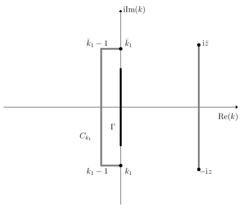
Figure 2. The contour $\Gamma$ and the branch cuts $C_{k_{1}}$ and $[-iz,i\bar{z}]$ in the complex $k$-plane.

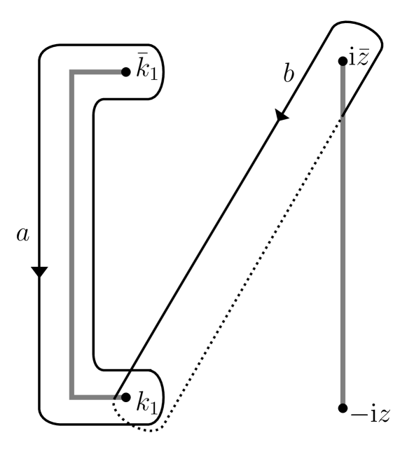
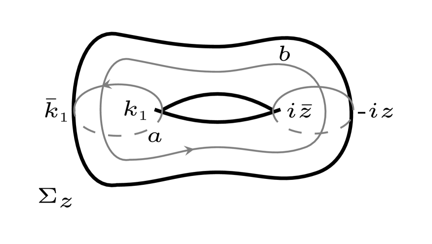
Figure 3. Two illustrations of the homology basis $\{a,b\}$ on the genus one Riemann surface $\Sigma_{z}$.

We let $\omega$ denote the unique holomorphic one-form on $\Sigma_{z}$ such that $\int_{a}\omega=1$. Then the period $B:=\int_{b}\omega\in\mathbb{C}$ has strictly positive imaginary part and we may define the Riemann-Siegel theta function $\Theta(v)\equiv\Theta(v|B)$ by

$$\Theta(v|B)=\sum_{N\in\mathbb{Z}}\exp\left[2\pi i\left(\frac{1}{2}N^{2}B+Nv\right)\right],\quad v\in\mathbb{C}.$$ (2.11)

Note that

$$\omega=A\frac{\mathrm{d}k}{y}\quad\text{and}\quad B=AZ,$$ (2.12)

where $A,Z\in\mathbb{C}$ are given by

$$A^{-1}=\int_{a}\frac{\mathrm{d}k}{y},\quad Z=\int_{b}\frac{\mathrm{d}k}{y}.$$ (2.13)

We let $\omega_{PQ}$ denote the Abelian differential of the third kind on $\Sigma_{z}$, which has simple poles at the two points $P,Q\in\Sigma_{z}$ with residues $+1$ and $-1$, respectively, and whose $a$-period vanishes. For $k\in\Sigma_{z}$, we have

$$\omega_{\zeta^{+}\zeta^{-}}(k)=\frac{y(\zeta^{+})dk}{(k-\zeta)y(k)}-\left(\int_{a}\frac{y(\zeta^{+})dk^{\prime}}{(k^{\prime}-\zeta)y(k^{\prime})}\right)\omega,$$

$$\omega_{\infty^{+}\infty^{-}}(k)=-\frac{kdk}{y(k)}+\left(\int_{a}\frac{k^{\prime}dk^{\prime}}{y(k^{\prime})}\right)\omega.$$ (2.14)

2.4. The Riemann surface $\Sigma^{\prime}$

As $z$ approaches the rotation axis, $\Sigma_{z}$ degenerates to the $z$-independent Riemann surface $\Sigma^{\prime}$ of genus zero defined by the equation

$$\mu=\sqrt{(k-k_{1})(k-\bar{k}_{1})}.$$ (2.15)

We use the branch cut $C_{k_{1}}$ in (2.10) to view $\Sigma^{\prime}$ as a two-sheeted cover of the complex $k$-plane. We denote the upper and lower sheets of $\Sigma^{\prime}$ by $\Sigma^{\prime+}$ and $\Sigma^{\prime-}$, respectively, characterized by $y\sim\pm k$ and $y\sim-k$ as $k\to\infty^{\pm}$. Letting $\omega^{\prime}_{PQ}$ denote the Abelian differential of the third kind on $\Sigma^{\prime}$ with simple poles at $P$ and $Q$, we have the following analog of (2.14):

$$\omega^{\prime}_{\zeta^{+}\zeta^{-}}=\frac{\mu(\zeta^{+})dk}{(k-\zeta)\mu(k)},\quad\omega^{\prime}_{\infty^{+}\infty^{-}}=-\frac{dk}{\mu(k)}.$$ (2.16)

3. Main results

Define the function $h(k)$ by

$$h(k)=-\frac{\text{arcsin}(2i\Omega k)}{\pi},$$ (3.1)

and note that $h(k)$ is smooth and real-valued for $k\in\Gamma$. We also define $u\equiv u(z)\in\mathbb{C}$ and $I\equiv I(z)\in\mathbb{R}$ by

$$u=\int_{\Gamma^{+}}h\omega,\quad I=\int_{\Gamma^{+}}h\omega_{\infty^{+}\infty^{-}},$$ (3.2)

where $\omega$ and $\omega_{\infty^{+}\infty^{-}}$ are the differentials on $\Sigma_{z}$ defined in Section 2 and we view $h$ as a function on $\Gamma^{+}$ in the natural way, i.e., by composing it with the projection $\Sigma_{z}\to\mathbb{C}$.

The next theorem, which is our main result, gives an explicit expression for the solution of the boundary value problem (2.8) and the associated metric functions in terms of the theta function $\Theta$ associated with the Riemann surface $\Sigma_{z}$.

Theorem 3.1 (Solution of the Neumann BVP).

Suppose $\Omega>0$ and $\rho_{0}>0$ are such that $2\Omega\rho_{0}<1$. Let $z=\rho+i\zeta$ with $\zeta>0$. Then the solution $f(z)\equiv f(\rho,\zeta)$ of the BVP (2.8) is given by

$$f(z)=\frac{\Theta(u-\int_{-iz}^{\infty^{-}}\omega|B)}{\Theta(u+\int_{-iz}^{\infty^{-}}\omega|B)}e^{I},$$ (3.3)

where $u$ and $I$ are defined in (3.2). Moreover, the associated metric functions $e^{2U}$ and $a$ are given by

$$e^{2U(z)}=\frac{Q(0)}{Q(u)}e^{I},\quad a(z)=a_{0}-\frac{\rho}{Q(0)}\left(\frac{\Theta\left(u+\int_{-iz}^{\infty^{-}}\omega+\int_{i\bar{z}}^{\infty^{-}}\omega|B\right)}{Q(0)\Theta\left(u+\int_{-iz}^{i\bar{z}}\omega|B\right)}-Q(u)\right)e^{-I},$$ (3.4)

where $a_{0}=-\frac{1}{2\Omega}$ and $Q(v)$ is defined by

$$Q(v)=\frac{\Theta\left(v+\int^{\infty^{-}}_{-iz}\omega|B\right)\Theta\left(v+\int^{\infty^{-}}_{i\bar{z}}\omega|B\right)}{\Theta\left(v|B\right)\Theta\left(v+\int_{-iz}^{i\bar{z}}\omega|B\right)},\quad v\in\mathbb{C}.$$ (3.5)

Finally, the metric function $e^{2\kappa}$ is given by

$$e^{2\kappa(z)}=K_{0}\frac{\Theta\left(u|B\right)\Theta\left(u+\int^{i\bar{z}}_{-iz}\omega|B\right)}{\Theta\left(0|B\right)\Theta\left(\int^{i\bar{z}}_{-iz}\omega|B\right)}e^{L^{reg}},$$ (3.6)

where $K_{0}$ and $L^{reg}$ are given by

$$K_{0}= \;\exp\left(-\frac{1}{2}\int_{\Gamma}\mathrm{d}\kappa_{1}h(\kappa_{1})\int_{\Gamma}^{\prime}h(\kappa_{2})\left(\frac{\partial\omega^{\prime}_{\kappa^{+}_{1}\kappa^{-}_{1}}}{\partial\kappa_{1}}(\kappa_{2}^{+})-\frac{\mathrm{d}\kappa_{2}}{(\kappa_{2}-\kappa_{1})^{2}}\right)\right),$$ (3.7)

$$L^{reg}= \;\frac{1}{2}\bigg{\{}\int_{\Gamma}d\kappa_{1}h(\kappa_{1})\int_{\Gamma}^{\prime}h(\kappa_{2})\bigg{(}\frac{\frac{\mathrm{d}y}{\mathrm{d}k}(\kappa_{1}^{+})(\kappa_{2}-\kappa_{1})+y(\kappa_{1}^{+})-y(\kappa_{2}^{+})}{(\kappa_{2}-\kappa_{1})^{2}y(\kappa_{2}^{+})}\bigg{)}d\kappa_{2}$$

$$-\bigg{(}\int_{\Gamma}^{\prime}d\kappa_{1}h(\kappa_{1})\int_{a}\frac{\frac{\mathrm{d}y}{\mathrm{d}k}(\kappa_{1}^{+})(\kappa-\kappa_{1})+y(\kappa_{1}^{+})}{(\kappa-\kappa_{1})^{2}y(\kappa)}d\kappa\bigg{)}\bigg{(}\int_{\Gamma}h(\kappa_{2})\omega(\kappa_{2}^{+})\bigg{)}\bigg{\}},$$ (3.8)

and a prime on an integral along $\Gamma$ means that the integration contour should be slightly deformed before evaluation so that the singularity at $\kappa_{1}=\kappa_{2}$ is avoided.

Remark 3.2 (Solution for $\zeta\leq 0$).

Theorem 3.1 provides expressions for the Ernst potential and the metric functions for $\zeta>0$. If $\rho>\rho_{0}$, these expressions extend continuously to $\zeta=0$. For negative $\zeta$, analogous expressions follow immediately from the equatorial symmetry. In this way, the solution of the BVP (2.8) is obtained in all of the exterior disk domain $\mathcal{D}$.

Remark 3.3 (The assumption $2\Omega\rho_{0}<1$).

We have stated Theorem 3.1 under the assumption that $2\Omega\rho_{0}<1$. If the rotation speed $\Omega$ and/or the radius $\rho_{0}$ are so large that $2\Omega\rho_{0}\geq 1$, then the branch points $k_{1}$ and $\bar{k}_{1}$ lie on $\Gamma$. Nevertheless, the formulas of Theorem 3.1 can easily be adjusted to include these (possibly singular) solutions.

Remark 3.4 (Solution in terms of elliptic theta functions).

The Ernst potential $f(z)$ given in (3.3) can be alternatively expressed in terms of the elliptic theta function $\theta_{3}$ by

$$f(z)=\frac{\theta_{3}\big{(}\frac{\pi(-\int_{-iz}^{\infty^{-}}\omega+u)}{B};e^{-\frac{\pi i}{B}}\big{)}}{\theta_{3}\big{(}\frac{\pi(\int_{-iz}^{\infty^{-}}\omega+u)}{B};e^{-\frac{\pi i}{B}}\big{)}}\exp\bigg{(}I+\frac{4\pi i\int_{-iz}^{\infty^{-}}\omega}{B}\bigg{)}.$$ (3.9)

The metric functions $e^{2U}$, $a$, and $\kappa$ can also be expressed in terms of elliptic theta functions in a similar way.

Remark 3.5 (Behavior at the rim of the disk).

The Ernst potential $f$ and the metric functions $e^{2U}$, $a$ and $e^{2\kappa}$ given in Theorem 3.1 are smooth functions of $(\rho,\zeta)$ in the open domain $\mathcal{D}$. They are bounded on $\mathcal{D}$ and extend smoothly to the interior $\{(\rho,0)\,|\,0<\rho<\rho_{0}\}$ of the disk from both above and below. Moreover, they extend continuously to the rim of the disk (i.e., to the point $(\rho,\zeta)=(\rho_{0},0)$), but they do not, in general, have $C^{1}$ extensions to this point (cf. Figures 4-6). In fact, an analysis shows that the boundary values of $e^{2U}$ and of its partial derivatives $\partial_{\rho}e^{2U}$ and $\partial_{\zeta}e^{2U}$ on the upper or lower side of the disk extend continuously to the rim of the disk. However, if $\zeta=0$ and $\rho\downarrow\rho_{0}$, then we only have

$$\frac{\partial e^{2U}}{\partial\rho}(\rho,0)=O\bigg{(}\frac{1}{\sqrt{\rho-\rho_{0}}}\bigg{)},\qquad\frac{\partial e^{2U}}{\partial\zeta}(\rho,0)=O\bigg{(}\frac{1}{\sqrt{\rho-\rho_{0}}}\bigg{)}.$$

Similarly, it can be shown that $a(z)$ and $e^{2\kappa}$ are continuous but not $C^{1}$ at $(\rho_{0},0)$, and that the partial derivatives $\partial_{\rho}a(z)$, $\partial_{\zeta}a(z)$, $\partial_{\rho}e^{2\kappa}(z)$, and $\partial_{\zeta}e^{2\kappa}(z)$ are $O(|z-\rho_{0}|^{-1/2})$ as $z\to\rho_{0}$.

3.1. Solution near the rotation axis

As $z$ approaches the rotation axis (i.e., as $\rho\to 0$), the Riemann surface $\Sigma_{z}$ degenerates to the genus zero surface $\Sigma^{\prime}$. We define the quantities $J^{\prime}\equiv J^{\prime}(\zeta)\in\mathbb{R}$ and $d\equiv d(\zeta)\in i\mathbb{R}_{-}$ for $\zeta>0$ by

$$J^{\prime}=\mu(\zeta^{+})\int_{\Gamma}\frac{h(k)}{\mu(k^{+})}\frac{dk}{k-\zeta},\quad d=2i\Omega(\zeta-\mu(\zeta^{+})).$$ (3.10)

where, by (2.15),

$$\mu(\zeta^{+})=\sqrt{\zeta^{2}+\frac{1}{4\Omega^{2}}}>0,\quad\zeta>0,$$

and

$$\mu(k^{+})=\sqrt{-|k|^{2}+\frac{1}{4\Omega^{2}}}>0,\quad k\in\Gamma.$$

The following result gives the asymptotic behavior of $f$ and the metric functions near the rotation axis.

Theorem 3.6 (Solution near the rotation axis).

Let $\zeta>0$. Under the assumptions of Theorem 3.1, the following asymptotic formulas hold as $\rho\downarrow 0$:

• The Ernst potential $f(z)$ satisfies

  $$f(\rho+i\zeta)=f(i\zeta)+O(\rho^{2}),$$ (3.11)

  where

  $$f(i\zeta)=\frac{1+e^{J^{\prime}}d}{e^{J^{\prime}}+d}.$$ (3.12)

• The metric functions $e^{2U}$, $a$, and $e^{2\kappa}$ satisfy

  $$e^{2U(\rho+i\zeta)}=e^{2U(i\zeta)}+O(\rho^{2}),\quad a(\rho+i\zeta)=O(\rho^{2}),\quad e^{2\kappa(\rho+i\zeta)}=1+O(\rho^{2}),$$ (3.13)

  where

  $$e^{2U(i\zeta)}=\frac{(1-d^{2})e^{J^{\prime}}}{e^{2J^{\prime}}-d^{2}}.$$ (3.14)

Remark 3.7 (Neumann condition at $\rho=0$).

Using the results of Theorem 3.6, we can easily verify explicitly that the Ernst potential of Theorem 3.1 satisfies $\mathrm{Re\,}\partial_{\zeta}f_{\Omega}(+i0)=0$, that is, that the real part of the Neumann boundary condition in (2.8) holds at the center of the disk. Indeed, by (3.12), we have

$$\frac{\partial}{\partial\zeta}\bigg{|}_{\zeta=0^{+}}f(i\zeta)=\frac{\partial}{\partial\zeta}\bigg{|}_{\zeta=0^{+}}\frac{1+e^{J^{\prime}}d}{e^{J^{\prime}}+d}.$$ (3.15)

Furthermore, it follows from (3.10) that

$$\lim_{\zeta\downarrow 0}d=-i,\quad\lim_{\zeta\downarrow 0}\partial_{\zeta}d=2i\Omega,$$ (3.16)

and

$$\frac{\partial J^{\prime}}{\partial\zeta}\bigg{|}_{\zeta=0^{+}} =\lim_{\zeta\downarrow 0}\int_{\Gamma}\frac{h(k)}{\mu(k^{+})}\frac{\partial}{\partial\zeta}\frac{\sqrt{\zeta^{2}+\frac{1}{4\Omega^{2}}}}{k-\zeta}dk=\lim_{\zeta\downarrow 0}\int_{\Gamma}\frac{h(k)}{\mu(k^{+})}\frac{(1+4k\zeta\Omega^{2})dk}{4\Omega^{2}(k-\zeta)^{2}\sqrt{\zeta^{2}+\frac{1}{4\Omega^{2}}}}.$$

The Sokhotski-Plemelj formula gives

$$\frac{\partial J^{\prime}}{\partial\zeta}\bigg{|}_{\zeta=0^{+}} =\;\mathchoice{{\vbox{\hbox{$\textstyle-$}}\kern-4.86108pt}}{{\vbox{\hbox{$\scriptstyle-$}}\kern-3.25pt}}{{\vbox{\hbox{$\scriptscriptstyle-$}}\kern-2.29166pt}}{{\vbox{\hbox{$\scriptscriptstyle-$}}\kern-1.875pt}}\!\int_{\Gamma}\frac{h(k)}{\mu(k^{+})}\frac{dk}{2\Omega k^{2}}-\pi i\underset{k=0}{\text{Res\,}}\bigg{(}\frac{h(k)}{\mu(k^{+})}\frac{dk}{2\Omega k^{2}}\bigg{)}=0-\frac{1}{\mu(0^{+})}=-2\Omega,$$ (3.17)

where the contribution from the principal value integral vanishes because the function $h(k)$ is odd. Using (3.16) and (3.17) to compute the right-hand side of (3.15), we find

$$\partial_{\zeta}f(+i0)=2i\Omega.$$ (3.18)

On the other hand, by (2.6a) and (3.13), we have $\mathrm{Re\,}f_{\Omega}(i\zeta)=\mathrm{Re\,}f(i\zeta)$ for $\zeta>0$. Hence $\mathrm{Re\,}\partial_{\zeta}f_{\Omega}(+i0)=\mathrm{Re\,}\partial_{\zeta}f(+i0)=\mathrm{Re\,}(2i\Omega)=0$, which shows that the Neumann boundary condition indeed holds for the real part of $f_{\Omega}$ at $\rho=0$.

4. Numerical example

The formulas of Theorem 3.1 are convenient for numerical computation. Consider for example the following particular choice of the parameters $\rho_{0}$ and $\Omega$:

$$\rho_{0}=1,\qquad\Omega=\frac{3}{10}.$$

Then $k_{1}=-5i/3$ and the graphs of the Ernst potential and the metric functions given in Theorem 3.1 are displayed in Figures 4-6. It can be numerically verified to high accuracy that $f_{\Omega}$ satisfies the Neumann condition along the disk, and that the defining relations (2.7) between the metric functions $a,\kappa$, and the Ernst potential $f$ are valid. Similar graphs and numerical results are obtained also for other choices of the parameters $\rho_{0}$ and $\Omega$ with $2\Omega\rho_{0}<1$.

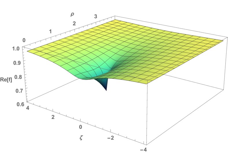
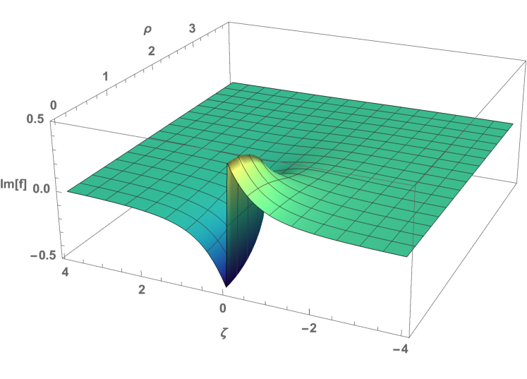
Figure 4. The real and the imaginary parts of the Ernst potential $f$.

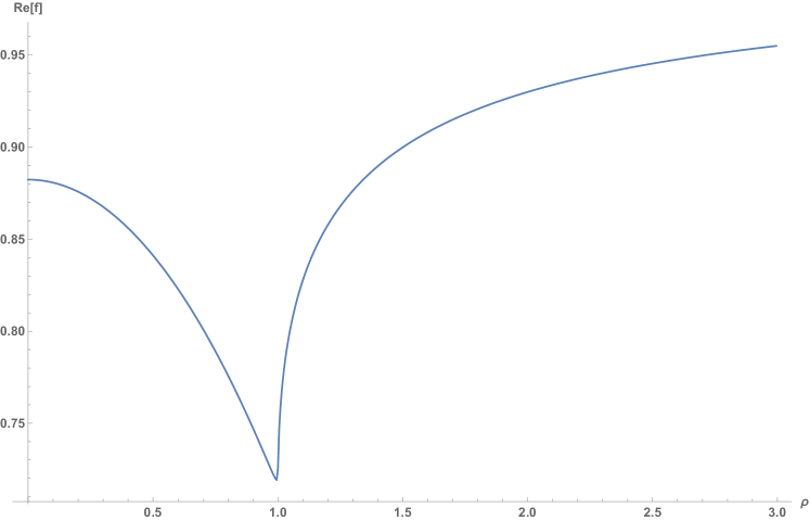
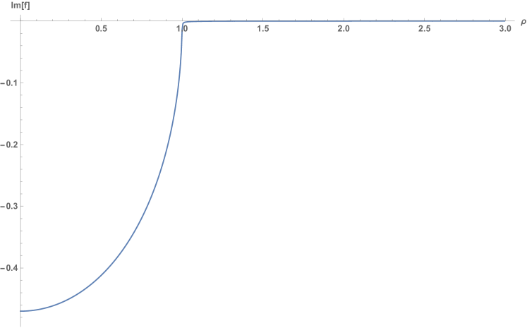
Figure 5. The real and imaginary parts of the Ernst potential $f(\rho+i0)$ on the equatorial plane $\zeta=+0$.

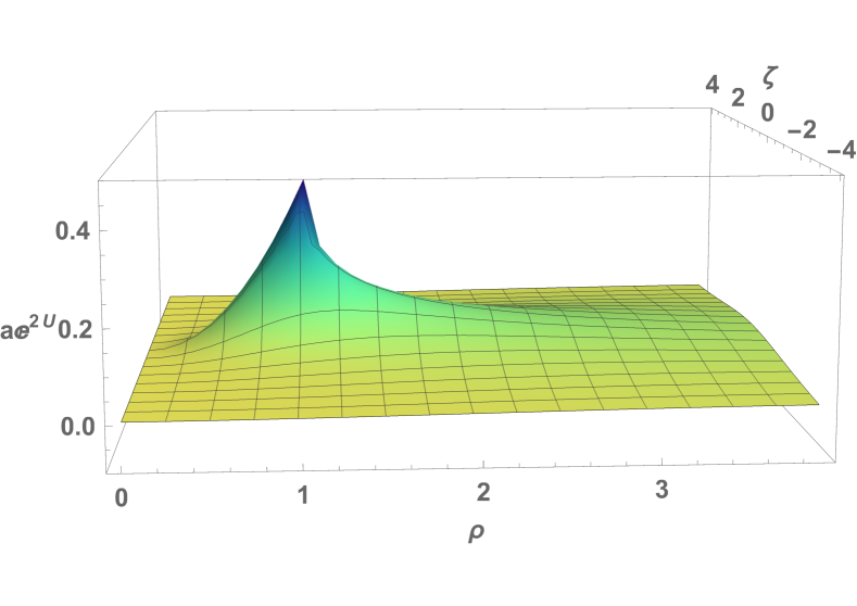
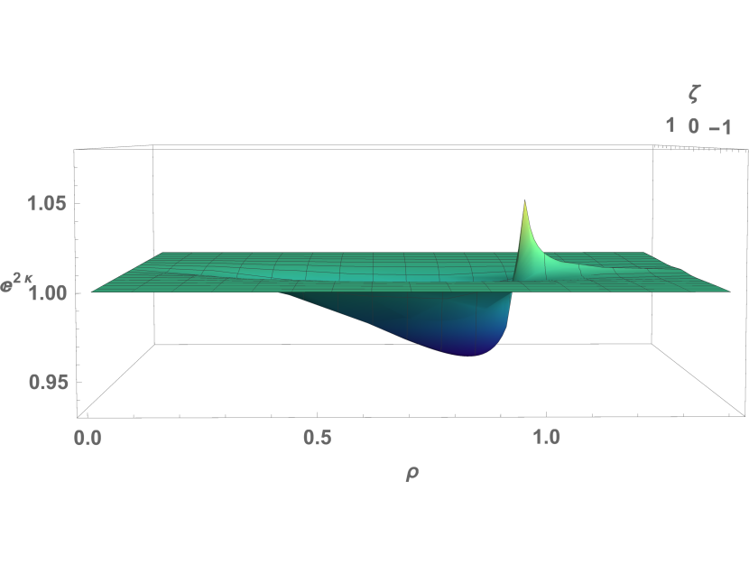
Figure 6. The metric functions $ae^{2U}$ and $e^{2\kappa}$.

5. Lax pair and spectral theory

5.1. Lax pair

The stationary Ernst equation (2.5) admits the Lax pair

$$\begin{split}\Phi_{z}(z,k)&=U(z,k)\Phi(z,k),\\ \Phi_{\bar{z}}(z,k)&=V(z,k)\Phi(z,k),\end{split}$$ (5.1)

where $z=\rho+i\zeta$, $\Phi(z,k)$ denotes the $2\times 2$ matrix-valued eigenfuntion, and $U$, $V$ are defined by

$$U=\frac{1}{f+\bar{f}}\begin{pmatrix}\bar{f}_{z}&\lambda\bar{f}_{z}\\ \lambda f_{z}&f_{z}\\ \end{pmatrix},\quad\quad V=\frac{1}{f+\bar{f}}\begin{pmatrix}\bar{f}_{\bar{z}}&\frac{1}{\lambda}\bar{f}_{\bar{z}}\\ \frac{1}{\lambda}f_{\bar{z}}&f_{\bar{z}}\\ \end{pmatrix},$$ (5.2)

with

$$\lambda=\sqrt{\frac{k-i\bar{z}}{k+iz}}.$$ (5.3)

For each $z$, $\Phi(z,\cdot)$ defines a map from $\mathscr{S}_{z}$ to the space of $2\times 2$ matrices, where $\mathscr{S}_{z}$ denotes the genus zero Riemann surface defined by (5.3). We view $\mathscr{S}_{z}$ as a two-sheeted covering of the complex $k$-plane by introducing the branch cut $[-iz,i\bar{z}]$ from $-iz$ to $i\bar{z}$. The upper (lower) sheet of $\mathscr{S}_{z}$ is charactered by $\lambda\to 1$ ($\lambda\to-1$) as $k\to\infty$. As in the case of $\Sigma_{z}$ and $\Sigma^{\prime}$, we write $k^{+}$ and $k^{-}$ for the points in $\mathscr{S}_{z}$ which project onto $k\in\hat{\mathbb{C}}\setminus[-iz,i\bar{z}]$ and which lie on the upper and lower sheets of $\mathscr{S}_{z}$, respectively. We let $\Gamma^{+}$ and $\Gamma^{-}$ denote the coverings of $\Gamma$ on the upper and lower sheets of $\mathscr{S}_{z}$, respectively. For a $2\times 2$-matrix $M$, we denote the first and second columns of $M$ by $[M]_{1}$ and $[M]_{2}$, respectively.

Equation (5.1) can be rewritten in differential form as

$$\mathrm{d}\Phi=W\Phi,$$ (5.4)

where the one-form $W$ is defined by

$$\begin{split}W&=\frac{1}{f+\bar{f}}\begin{pmatrix}\bar{f}_{\rho}&\frac{1}{2}\left[\left(\frac{1}{\lambda}+\lambda\right)\bar{f}_{\rho}+i\left(\frac{1}{\lambda}-\lambda\right)\bar{f}_{\zeta}\right]\vspace{10pt}\\ \frac{1}{2}\left[\left(\frac{1}{\lambda}+\lambda\right)f_{\rho}+i\left(\frac{1}{\lambda}-\lambda\right)f_{\zeta}\right]&f_{\rho}\\ \end{pmatrix}\mathrm{d}\rho\\ &\quad+\frac{1}{f+\bar{f}}\begin{pmatrix}\bar{f}_{\zeta}&\frac{1}{2}\left[\left(\frac{1}{\lambda}+\lambda\right)\bar{f}_{\zeta}-i\left(\frac{1}{\lambda}-\lambda\right)\bar{f}_{\rho}\right]\vspace{10pt}\\ \frac{1}{2}\left[\left(\frac{1}{\lambda}+\lambda\right)f_{\zeta}-i\left(\frac{1}{\lambda}-\lambda\right)f_{\rho}\right]&f_{\zeta}\\ \end{pmatrix}\mathrm{d}\zeta\\ &=:W_{1}\mathrm{d}\rho+W_{2}\mathrm{d}\zeta.\end{split}$$ (5.5)

We normalize the eigenfunction $\Phi$ by imposing the conditions

$$\lim_{z\to i\infty}\left[\Phi(z,k^{-})\right]_{1}=\begin{pmatrix}1\\ 1\end{pmatrix},\quad\lim_{z\to i\infty}\left[\Phi(z,k^{+})\right]_{2}=\begin{pmatrix}1\\ -1\end{pmatrix}$$ (5.6)

for all $k\in\hat{\mathbb{C}}$. As a consequence, $\Phi(z,k)$ admits the symmetries

$$\Phi(z,k^{+})=\sigma_{3}\Phi(z,k^{-})\sigma_{1},\quad\Phi(z,k^{+})=\sigma_{1}\overline{\Phi(z,\overline{k}^{+})}\sigma_{3},$$ (5.7)

where $\{\sigma_{j}\}_{1}^{3}$ are the standard Pauli matrices.

We henceforth suppose that $f(z)$ is a solution of the BVP (2.8). Physically, the possibly empty set of points where $\mathrm{Re\,}f=0$ constitutes the ergospheres of the spacetime. The matrices $U$ and $V$ in the Lax pair (5.1) are, in general, singular at these points and this may give rise to singularities of $\Phi$. On the other hand, points where $\det\Phi=0$ are related to the presence of solitons (cf. [14]). It is natural to expect the solution of the boundary value problem (2.8) to be free of ergospheres and solitons (at least for small values of $\Omega$). We will therefore henceforth make the assumption that

$$\mathrm{Re\,}f>0\quad\text{and}\quad\det\Phi\neq 0$$ (5.8)

throughout the spacetime. The consistency of this assumption can be ascertained once the final solution has been constructed. By integrating both sides of (5.4) from $i\infty$ to $z$ and using (5.8), it can be confirmed that $\Phi(z,k)$ is a well-defined analytic function of $k\in\mathscr{S}_{z}\setminus(\Gamma^{+}\cup\Gamma^{-})$ for any fixed $z$, see [12].

Let $\Phi_{\Omega}$ denote the co-rotating counterpart of $\Phi$. The Lax pair equations (5.1) and the conditions (5.6) retain their form in the co-rotating frame with $f$ and $\Phi$ replaced by $f_{\Omega}$ and $\Phi_{\Omega}$. It is proved in [13] that $\Phi_{\Omega}$ is related to $\Phi$ by

$$\Phi_{\Omega}(z,k)=\Lambda(z,k)\Phi(z,k),$$

where

$$\Lambda(z,k)=(1+\Omega a)\mathbb{I}-\Omega\rho e^{-2U}\sigma_{3}+i(k+iz)\Omega e^{-2U}(-\sigma_{3}+\lambda(z,k)\sigma_{1}\sigma_{3}),\quad k\in\mathscr{S}_{z},$$

and $\mathbb{I}$ denote the $2\times 2$ identity matrix.

5.2. The main RH problem

The following lemma can be found in [12].

Lemma 5.1.

For $k\in\mathbb{C}$, $\Phi(i\zeta,k)$ can be expressed in terms of $f(i\zeta)$ and the spectral functions $F(k)$ and $G(k)$ as follows:

$$\Phi(i\zeta,k^{+}) =\begin{pmatrix}\overline{f(i\zeta)}&1\\ f(i\zeta)&-1\\ \end{pmatrix}\mathcal{A}(k),\quad\zeta>0,$$

$$\Phi(i\zeta,k^{-}) =\begin{pmatrix}1&\overline{f(i\zeta)}\\ 1&-f(i\zeta)\\ \end{pmatrix}\sigma_{1}\mathcal{A}(k)\sigma_{1},\quad\zeta>0,$$

$$\Phi(i\zeta,k^{+}) =\begin{pmatrix}\overline{f(i\zeta)}&1\\ f(i\zeta)&-1\\ \end{pmatrix}\sigma_{1}\mathcal{A}(k)\sigma_{1},\quad\zeta<0,$$

$$\Phi(i\zeta,k^{-}) =\begin{pmatrix}1&\overline{f(i\zeta)}\\ 1&-f(i\zeta)\\ \end{pmatrix}\mathcal{A}(k),\quad\zeta<0,$$

where $\mathcal{A}(k)$ is defined by

$$\mathcal{A}(k)=\begin{pmatrix}F(k)&0\\ G(k)&1\\ \end{pmatrix}$$ (5.9)

and the spectral functions $F(k)$ and $G(k)$ have the following properties:

• $F(k)$ and $G(k)$ descend to functions on $\hat{\mathbb{C}}$, namely when viewed as functions on $\mathscr{S}_{z}$, they satisfy

  $$F(k^{+})=F(k^{-}),\quad G(k^{+})=G(k^{-}),\quad k\in\hat{\mathbb{C}}.$$ (5.10)

• $F(k)$ and $G(k)$ are analytic for $k\in\mathbb{C}\backslash\Gamma$.

• $F(k)=\overline{F(\overline{k})}$ and $G(k)=-\overline{G(\overline{k})}$ for $k\in\mathbb{C}\backslash\Gamma$.

• As $k\to\infty$,

  $$F(k)=1+O(k^{-1}),\quad G(k)=O(k^{-1}).$$ (5.11)

The jumps of the function $\Phi(z,k)$ across $\Gamma^{+}$ and $\Gamma^{-}$ can be expressed in terms of $F(k)$ and $G(k)$. In fact, let $g_{+}(k)$ and $g_{-}(k)$ denote the boundary values of a function $g(k)$ on the right and left sides of $\Gamma$, respectively. Then $\Phi(z,k)$ satisfies (see [12, 13])

$$\begin{cases}\Phi_{-}(z,k)=\Phi_{+}(z,k)D(k),&k\in\Gamma^{+},\\ \Phi_{-}(z,k)=\Phi_{+}(z,k)\sigma_{1}D(k)\sigma_{1},&k\in\Gamma^{-},\end{cases}$$ (5.12)

where $D$ is defined by

$$D(k)=\begin{pmatrix}F_{+}(k)&0\\ G_{+}(k)&1\\ \end{pmatrix}^{-1}\begin{pmatrix}F_{-}(k)&0\\ G_{-}(k)&1\\ \end{pmatrix}.$$ (5.13)

5.3. The global relation

Since $f$ is equatorially symmetric, the values of $F(k)$ and $G(k)$ on the left and right sides of $\Gamma$ satisfy an important relation called the global relation.

Lemma 5.2 (Global relation).

The spectral functions $F(k)$ and $G(k)$ satisfy

$$\overline{\mathcal{A}_{+}(k)}\sigma_{1}\overline{\mathcal{A}^{-1}_{+}(k)}\sigma_{1}=\sigma_{1}\mathcal{A}_{-}(k)\sigma_{1}\mathcal{A}_{-}^{-1}(k),\qquad k\in\Gamma,$$ (5.14)

where $\mathcal{A}_{+}(k)$ and $\mathcal{A}_{-}(k)$ denote the values of $\mathcal{A}(k)$ on the right and left sides of $\Gamma$, respectively.

Proof.

See [12, Proposition 4.3]. ∎

5.4. An additional relation

The fact that $f_{\Omega}$ obeys a Neumann condition along the disk implies that $F(k)$ and $G(k)$ satisfy an additional relation beyond the global relation.

We use the superscripts $L$ and $R$ on a function of $k$ to indicate that this function should be evaluated with $k$ lying on the left or right side of the branch cut $[-iz,i\bar{z}]$, respectively. If one of the superscripts $L$ or $R$ is present, we always assume that the evaluation point $k$ lies to the right of $\Gamma$. The latter specification is needed when $z=\rho+i0$ so that the branch cut $[-iz,i\bar{z}]$ runs infinitesimally close to $\Gamma$.

Lemma 5.3 (An additional relation).

The function $\mathcal{A}(k)\sigma_{1}\mathcal{A}^{-1}(k)$ satisfies

$$\begin{split}\big{[}\mathcal{B}^{-1}\Lambda^{-1}&(+i0,k^{+})\sigma_{1}\overline{\Lambda(+i0,k^{+})}\overline{\mathcal{B}}\sigma_{1}\big{]}\big{[}\sigma_{1}\overline{\mathcal{A}_{+}(k)}\sigma_{1}\overline{\mathcal{A}^{-1}_{+}(k)}\sigma_{1}\big{]}\\ &=-\big{[}\mathcal{A}_{+}(k)\sigma_{1}\mathcal{A}_{+}^{-1}(k)\big{]}\big{[}\mathcal{B}^{-1}\Lambda^{-1}(+i0,k^{+})\sigma_{1}\overline{\Lambda(+i0,k^{+})}\overline{\mathcal{B}}\sigma_{1}\big{]},\quad k\in\Gamma,\end{split}$$ (5.15)

where the matrix $\mathcal{B}$ is defined by

$$\mathcal{B}=\begin{pmatrix}\overline{f(+i0)}&1\\ f(+i0)&-1\end{pmatrix}.$$

Proof.

We let $W_{\Omega}=W_{1\Omega}\mathrm{d}\rho+W_{2\Omega}\mathrm{d}\zeta$ denote the co-rotating analog of the one-form $W$ defined in (5.5). The restriction of $W_{\Omega}$ to the upper side of the disk is given by $W_{1\Omega}(\rho+i0,k)\mathrm{d}\rho$. Evaluating the identity

$$\lambda(z,k^{+})=\frac{1}{\lambda(z,(-k+2\zeta)^{+})}$$

at $z=\rho+i0$, we find

$$\lambda^{R}(\rho+i0,k^{+})=\frac{1}{\lambda^{L}(\rho+i0,\bar{k}^{+})},\qquad k\in\Gamma.$$ (5.16)

Inserting the Neumann condition for $f_{\Omega}$ into the expression (5.5) for $W_{1\Omega}$ and using (5.16) as well as the symmetry $\lambda(z,k^{\pm})=1/\overline{\lambda(z,\bar{k}^{\pm})}$, we deduce that

$$W_{1\Omega}^{R}(\rho+i0,k^{+})=\sigma_{1}\overline{W_{1\Omega}^{L}(\rho+i0,k^{+})}\sigma_{1},\qquad\rho\in(0,\rho_{0}),\ k\in\Gamma.$$

Thus, by (5.4), there exists a $2\times 2$-matrix valued, $\rho$-independent function $\mathcal{K}(k)$ such that

$$\overline{\Phi_{\Omega}^{L}(\rho+i0,k^{+})}=\sigma_{1}\Phi_{\Omega}^{R}(\rho+i0,k^{+})\mathcal{K}(k),\qquad k\in\Gamma.$$ (5.17)

It follows from the first symmetry in (5.7) that $\sigma_{1}\mathcal{K}=-\mathcal{K}\sigma_{1}$ on $\Gamma$ (cf. [12, Proposition 5.2]). The lemma then follows by evaluating (5.17) at $\rho=0$ and using Lemma 5.1. ∎

5.5. The auxiliary RH problem

By combining the global relation (5.14) with the relation of Lemma 5.3, we can formulate a RH problem for the $2\times 2$-matrix valued function $\mathcal{M}(k)$ by

$$\mathcal{M}(k)=\mathcal{A}(k)\sigma_{1}\mathcal{A}^{-1}(k)=\begin{pmatrix}-G(k)&F(k)\\ \frac{1-G^{2}(k)}{F(k)}&G(k)\\ \end{pmatrix}.$$ (5.18)

Lemma 5.4.

Suppose $f$ is a solution of the BVP (2.8). Then the spectral functions $F(k)$ and $G(k)$ are given by

$$F(k)=\mathcal{M}_{12}(k),\quad G(k)=\mathcal{M}_{22}(k),\quad k\in\mathbb{C},$$ (5.19)

where $\mathcal{M}$ is the unique solution of the following RH problem:

• $\mathcal{M}(k)$ is analytic for $k\in\mathbb{C}\backslash\Gamma$.

• Across $\Gamma$, $\mathcal{M}(k)$ satisfies the jump condition

  $$\mathcal{S}(k)\mathcal{M}_{-}(k)=-\mathcal{M}_{+}(k)\mathcal{S}(k),\quad k\in\Gamma,$$ (5.20)

  where $\mathcal{S}(k)$ is defined by

  $$\mathcal{S}(k)=\begin{pmatrix}0&1\\ -1&4ik\Omega\\ \end{pmatrix},\quad k\in\mathbb{C}.$$ (5.21)

• $\mathcal{M}(k)$ has at most logarithmic singularities at the endpoints of $\Gamma$.

• $\mathcal{M}(k)$ has the asymptotic behavior

  $$\mathcal{M}(k)=\sigma_{1}+O(k^{-1}),\quad k\to\infty.$$ (5.22)

Moveover,

$$\mathrm{tr}\,{\mathcal{(MS)}=0},\quad k\in\hat{\mathbb{C}}.$$ (5.23)

Proof.

Since $\det\Phi(z,k)=-2e^{2U(z)}F(k)$ (see [13, Eq. (2.65)]), the assumptions (5.8) imply that $F(k)$ never vanishes. The analyticity of $\mathcal{M}(k)$ for $k\in\hat{\mathbb{C}}\backslash\Gamma$ then follows from the analyticity of $F(k)$ and $G(k)$ (see Lemma 5.1). Combining the global relation (5.14) with relation (5.15), we find the jump relation (5.20) with $\mathcal{S}(k)$ given by

$$\mathcal{S}(k)=\mathcal{B}^{-1}\Lambda^{-1}(+i0,k^{+})\sigma_{1}\overline{\Lambda(+i0,k^{+})}\overline{\mathcal{B}}\sigma_{1},\quad k\in\Gamma.$$ (5.24)

By inserting the definitions of $\mathcal{B}$ and $\Lambda$, we see that this expression simplifies to (5.21) when $k\in\Gamma$. The asymptotic behavior of $\mathcal{M}$ in (5.22) is a consequence of the asymptotics of $F$ and $G$ in (5.11). Define $\mathcal{R}(\rho,k)$ by

$$\mathcal{R}=\Phi^{-1}_{\Omega}(\rho+i0,k^{+})\sigma_{1}\Phi_{\Omega}(\rho-i0,k^{+}).$$ (5.25)

As in the proof of the existence of the matrix $\mathcal{K}(k)$ in (5.17), we deduce that $\mathcal{R}$ is independent of $\rho$. Then (5.23) follows by evaluating $\mathcal{R}$ at $\rho=\rho_{0}$ and $\rho=0$. ∎

5.6. Solution of the auxiliary RH problem

By solving the RH problem of Lemma 5.4, we can obtain explicit expressions for $F(k)$ and $G(k)$.

Let $d_{1}(k)$ denote the unique meromorphic function on $\Sigma^{\prime}$ which is analytic except for a simple pole at $\infty^{-}$ with residue $4\Omega i$ and a simple zero at $\infty^{+}$, i.e.,

$$d_{1}(k)=2\Omega i(k-\mu(k))$$

where $\mu(k)=\sqrt{k^{2}+1/(4\Omega^{2})}$ is the square root defined in (2.15). Define the scalar-valued function $E(k)$ on $\Sigma^{\prime}$ by

$$E(k)=e^{\mu(k)\int_{\Gamma}\frac{h(s)}{\mu(s^{+})}\frac{ds}{s-k}},$$ (5.26)

Then $E(k)$ is an analytic function of $k\in\Sigma^{\prime}\setminus(\Gamma^{+}\cup\Gamma^{-})$ such that $(i)$ $d_{1}E_{-}+d_{1}^{-1}E_{+}=0$ for $k\in\Gamma^{+}\cup\Gamma^{-}$, $(ii)$ $E(k)$ has logarithmic singularities at the endpoints of $\Gamma^{+}$ and $\Gamma^{-}$, $(iii)$ $E(k^{+})=\overline{E(\bar{k}^{+})}$, $(iv)$ $E(k^{+})=E(k^{-})^{-1}$, and $(v)$ $E(k^{+})=1+O(k^{-1})$ as $k\to\infty$, where we have used the symmetry $h(k)=-h(-k)$ to see that $E(\infty^{+})=1$.

Lemma 5.5.

The spectral functions $F(k)$ and $G(k)$ are given by

$$\begin{cases}F(k)=\frac{i}{4\Omega\mu(k^{+})}\Big{(}\frac{d_{1}(k^{+})}{E(k^{+})}-\frac{E(k^{+})}{d_{1}(k^{+})}\Big{)},\vspace{1mm}\\ G(k)=\frac{i}{4\Omega\mu(k^{+})}\Big{(}\frac{1}{E(k^{+})}-E(k^{+})\Big{)},\end{cases}\quad k\in\mathbb{C}\setminus\Gamma.$$ (5.27)

Proof.

The matrix $\mathcal{S}$ in (5.20) can be diagonalized as $\mathcal{S}(k)=T(k)\mathcal{D}(k)T(k)^{-1}$, where

$$\mathcal{D}(k)=\begin{pmatrix}d_{1}(k)&0\\ 0&d_{2}(k)\end{pmatrix},\qquad T(k)=\begin{pmatrix}d_{2}(k)&d_{1}(k)\\ 1&1\end{pmatrix},$$

and $d_{2}(k):=d_{1}(k)^{-1}=2\Omega i(k+\mu(k))$. We view $\mathcal{D}(k)$ and $\mathcal{T}(k)$ as functions on the Riemann surface $\Sigma^{\prime}$ and note that $|d_{1}|=1$ on $\Gamma^{\pm}$. The inverse

$$T(k)^{-1}=\frac{1}{4\Omega i\mu(k)}\begin{pmatrix}1&-d_{1}(k)\\ -1&d_{2}(k)\end{pmatrix}$$

is analytic on $\Sigma^{\prime}$ except for simple poles at $k_{1},\bar{k}_{1}$. It follows from Lemma 5.4 that the $2\times 2$-matrix valued function $\mathcal{N}(k)$ defined by

$$\mathcal{N}(k)=T(k)^{-1}\mathcal{M}(k)T(k)$$ (5.28)

is an analytic $2\times 2$-matrix valued function of $k\in\Sigma^{\prime}\setminus(\Gamma^{+}\cup\Gamma^{-}\cup k_{1}\cup\bar{k}_{1}\cup\infty^{+}\cup\infty^{-})$ such that $(i)$ $\mathcal{N}(k)$ satisfies the jump condition $\mathcal{D}\mathcal{N}_{-}+\mathcal{N}_{+}\mathcal{D}=0$ for $k\in\Gamma^{+}\cup\Gamma^{-}$, $(ii)$ $\mathcal{N}(k)$ has at most simple poles at $k_{1}$ and $\bar{k}_{1}$, $(iii)$ $\mathrm{tr}\,\mathcal{N}(k)=0$ and $\det\mathcal{N}(k)=-1$, and $(iv)$ $\mathcal{N}(k^{+})=\sigma_{1}\mathcal{N}(k^{-})\sigma_{1}$, In terms of $\mathcal{N}$, the identity $\mathrm{tr}\,(\mathcal{S}\mathcal{M})=0$ in (5.23) becomes

$$0=\mathrm{tr}\,(\mathcal{S}\mathcal{M})=\mathrm{tr}\,(\mathcal{D}\mathcal{N})=(d_{1}(k)-d_{2}(k))\mathcal{N}_{11}(k),$$

showing that the $(11)$ entry $\mathcal{N}_{11}(k)$ of $\mathcal{N}(k)$ vanishes identically. Since $\mathrm{tr}\,\mathcal{N}(k)=0$ and $\det\mathcal{N}=-1$, it follows that $\mathcal{N}_{22}(k)=0$ and $\mathcal{N}_{12}\mathcal{N}_{21}=1$. The $(12)$ entry $\mathcal{N}_{12}$ obeys the jump condition

$$d_{1}\mathcal{N}_{12-}+d_{2}\mathcal{N}_{12+}=0,\qquad k\in\Gamma^{+}\cup\Gamma^{-},$$

the symmetry $\mathcal{N}_{12}(k^{+})=\mathcal{N}_{12}(k^{-})^{-1}$, and the asymptotics $\mathcal{N}_{12}(k^{-})=4\Omega ik+O(1)$ as $k\to\infty$. It follows that the function $n(k)$ defined on $\Sigma^{\prime}$ by $n(k)=\mathcal{N}_{12}(k)E(k)^{-1}$ has no jump across $\Gamma^{+}\cup\Gamma^{-}$. Moreover, since

$$\mathcal{M}_{22}=\frac{\mathcal{N}_{12}+\mathcal{N}_{12}^{-1}}{2}+\frac{k}{2\mu(k)}(\mathcal{N}_{12}-\mathcal{N}_{12}^{-1}),$$ (5.29)

is analytic at $k_{1}$ and $\bar{k}_{1}$, we deduce that $\mathcal{N}_{12}$ (and hence also $n(k)$) actually is analytic at $k_{1}$ and $\bar{k}_{1}$. At the endpoints $(\pm i\rho_{0})^{+}$ and $(\pm i\rho_{0})^{-}$ of $\Gamma^{\pm}$, $n(k)$ has isolated singularities which are at most logarithmic; hence $n(k)$ is analytic also at these points. Consequently, $n(k)$ is the unique meromorphic function on $\Sigma^{\prime}$ with a simple pole with residue $4\Omega i$ at $\infty^{-}$ and a simple zero at $\infty^{+}$, that is, $n(k)=d_{1}(k)$. We conclude that

$$\mathcal{N}(k)=\begin{pmatrix}0&d_{1}(k)E(k)\\ d_{1}(k)^{-1}E(k)^{-1}&0\end{pmatrix}.$$

The expressions (5.27) follow from (5.19) and (5.28) by straightforward algebra. ∎

5.7. The Ernst potential on the rotation axis

Recalling that (see [13, p. 46])

$$F(\zeta)=\frac{1}{\mathrm{Re\,}f(i\zeta)},\qquad G(\zeta)=\frac{i\mathrm{Im\,}f(i\zeta)}{\mathrm{Re\,}f(i\zeta)},\qquad\zeta>0,$$

$$F(\zeta)=\frac{|f(i\zeta)|^{2}}{\mathrm{Re\,}f(i\zeta)},\qquad G(\zeta)=\frac{-i\mathrm{Im\,}f(i\zeta)}{\mathrm{Re\,}f(i\zeta)},\qquad\zeta<0,$$

we find the following expression for the value of the Ernst potential on the rotation axis:

$$f(i\zeta)=\begin{cases}\frac{1+G(\zeta)}{F(\zeta)}=\frac{1+d_{1}(\zeta^{+})E(\zeta^{+})}{d_{1}(\zeta^{+})+E(\zeta^{+})},\qquad\zeta>0,\\ \frac{F(\zeta)}{1+G(\zeta)}=\frac{d_{1}(\zeta^{+})+E(\zeta^{+})}{1+d_{1}(\zeta^{+})E(\zeta^{+})},\qquad\zeta<0.\end{cases}$$

Using that $E(\zeta^{+})=e^{J^{\prime}(\zeta)}$ and $d(\zeta)=d_{1}(\zeta^{+})$ for $\zeta>0$, where $J^{\prime}$ and $d$ are the functions defined in (3.10), we arrive at the expression (3.12) for $f(i\zeta)$. Since $J^{\prime}(\zeta)\in\mathbb{R}$ and $d_{1}(\zeta)\in i\mathbb{R}_{-}$ for $\zeta>0$, the expression (3.14) for $e^{2U(i\zeta)}$ follows by taking the real part of (3.12).

6. The scalar RH problem

Substitution of the expressions for $F(k)$ and $G(k)$ obtained in Lemma 5.5 into (5.13) gives an explicit expression for the jump matrix $D(k)$. Thus we have an effective solution of the BVP (2.8) in terms of the solution of the matrix RH problem (5.12). In what follows, we instead employ the main and auxiliary RH problems to formulate a scalar RH problem on the Riemann surface $\Sigma_{z}$. The solution of this scalar RH problem leads to the exact formulas of Theorem 3.1.

6.1. The functions $\mathcal{L}(z,k)$ and $\mathcal{Q}(z,k)$

Define $w(k)$ by

$$w(k)=-\frac{1}{2}\mathrm{tr}\,(\mathcal{S}(k))=-2ik\Omega,\quad k\in\mathbb{C}.$$

Introduce the $2\times 2$ matrix valued functions $\mathcal{L}$ and $\mathcal{Q}$ by

$$\mathcal{L}(z,k) =\Phi(z,k)\sigma_{1}\Phi^{-1}(z,k),\quad k\in\mathscr{S}_{z},$$ (6.1)

$$\mathcal{Q}(z,k) =-\Phi(z,k)\mathcal{A}^{-1}(k)\mathcal{S}(k)\mathcal{A}(k)\Phi^{-1}(z,k)-w(k)\mathbb{I},\quad k\in\mathscr{S}_{z}.$$ (6.2)

Lemma 6.1.

The functions $\mathcal{L}$ and $\mathcal{Q}$ have the following properties:

• $\mathcal{L}$ and $\mathcal{Q}$ satisfy the trace and determinant relations

  $$\mathrm{tr}\,\mathcal{Q}=0,\quad\mathrm{tr}\,\mathcal{L}=0,\quad\det\mathcal{L}=-1,\quad\det\mathcal{Q}=1-w^{2},$$ (6.3)

  and the symmetries

  $$\mathcal{Q}(z,k^{-})=-\sigma_{3}\mathcal{Q}(z,k^{+})\sigma_{3},\quad\mathcal{L}(z,k^{-})=\sigma_{3}\mathcal{L}(z,k^{+})\sigma_{3}.$$ (6.4)

• $\mathcal{Q}$ can be rewritten as

  $$\mathcal{Q}(z,k)=\Phi(z,k)\sigma_{1}\mathcal{A}^{-1}(k)\mathcal{S}(k)\mathcal{A}(k)\sigma_{1}\Phi^{-1}(z,k)+w(k)\mathbb{I}.$$ (6.5)

• $\mathcal{Q}$ has no jump across $\Gamma^{+}\cup\Gamma^{-}$, whereas $\mathcal{L}$ satisfies the jump conditions

  $$\begin{cases}(\mathcal{Q}+w\mathbb{I})\mathcal{L}_{-}=-\mathcal{L}_{+}(\mathcal{Q}+w\mathbb{I}),&k\in\Gamma^{+},\\ (\mathcal{Q}-w\mathbb{I})\mathcal{L}_{-}=-\mathcal{L}_{+}(\mathcal{Q}-w\mathbb{I}),&k\in\Gamma^{-}.\end{cases}$$ (6.6)

• $\mathcal{L}$ and $\mathcal{Q}$ anticommute, i.e., $\mathcal{Q}\mathcal{L}=-\mathcal{L}\mathcal{Q}$.

• The function $\hat{\mathcal{L}}$ defined by

  $$\hat{\mathcal{L}}=\mathcal{L}\begin{pmatrix}1&\mathcal{Q}_{11}\\ 0&\mathcal{Q}_{21}\\ \end{pmatrix},$$

  satisfies

  $$\hat{\mathcal{L}}_{22}^{2}-\mathcal{L}_{21}^{2}(w^{2}-1)=\mathcal{Q}^{2}_{21}.$$ (6.7)

• For each $z$, there exists a point $m_{1}\equiv m_{1}(z)\in\mathbb{C}$ such that

  $$\mathcal{Q}_{21}(z,k)=\frac{4i\Omega f}{f+\bar{f}}(k-m_{1}).$$ (6.8)

Proof.

The properties in (6.3) follow from the definitions of $\mathcal{L}$ and $\mathcal{Q}$ and the fact that $\det(\mathcal{S}+w\mathbb{I})=1-w^{2}$. The symmetries in (6.4) are a consequence of (5.7) and (5.23). The alternative expression (6.5) for $\mathcal{Q}$ follows from (5.23). Equations (5.12) and (5.13) imply that $\Phi\mathcal{A}^{-1}$ and $\Phi\sigma_{1}\mathcal{A}^{-1}$ do not jump across $\Gamma^{+}$ and $\Gamma^{-}$, respectively. Thus, by (6.2) and (6.5), $\mathcal{Q}$ does not jump across $\Gamma^{+}$ or $\Gamma^{-}$. Since, for $k\in\Gamma^{+}$,

$$(\mathcal{Q}_{-}+w\mathbb{I})\mathcal{L}_{-} =-\Phi_{-}\mathcal{A}^{-1}_{-}\mathcal{S}\mathcal{A}_{-}\sigma_{1}\Phi_{-}^{-1}=-\Phi_{-}\mathcal{A}^{-1}_{-}\mathcal{S}\mathcal{M}_{-}\mathcal{A}_{-}\Phi^{-1}_{-},$$ (6.9)

$$-\mathcal{L}_{+}(\mathcal{Q}_{+}+w\mathbb{I}) =\Phi_{+}\sigma_{1}\mathcal{A}^{-1}_{+}\mathcal{S}\mathcal{A}_{+}\Phi_{+}^{-1}=\Phi_{+}\mathcal{A}^{-1}_{+}\mathcal{M}_{+}\mathcal{S}\mathcal{A}_{+}\Phi_{+}^{-1},$$ (6.10)

the jump of $\mathcal{L}$ across $\Gamma^{+}$ is a consequence of (5.12) and (5.20). The jump of $\mathcal{L}$ across $\Gamma^{-}$ then follows from (6.4). Using (6.5), it follows from (5.23) that $\mathcal{L}\mathcal{Q}=-\mathcal{Q}\mathcal{L}$ and then (6.7) follows by direct computation. Since $\mathcal{Q}_{21}$ is an entire function of $k\in\mathbb{C}$, the expression for $\mathcal{Q}_{21}$ in (6.8) follows from the asymptotic formulas

$$\Phi(z,k^{+})=\begin{pmatrix}\overline{f(z)}&1\\ f(z)&-1\end{pmatrix}+O(k^{-1}),\quad\mathcal{A}(k)=\mathbb{I}+O(k^{-1}),\quad k\to\infty,$$ (6.11)

and Liouville’s theorem. ∎

6.2. The Riemann surface $\hat{\mathscr{S}}_{z}$ and the function $H(z,k)$

Let $\hat{\mathscr{S}}_{z}$ denote the double covering of $\mathscr{S}_{z}$ obtained by adding the cut $C_{k_{1}}$ from $k_{1}$ to $\overline{k}_{1}$ on both the upper and lower sheet of $\mathscr{S}_{z}$. Thus a point $(k,\pm\lambda,\pm\mu)$ on $\hat{\mathscr{S}}_{z}$ is specified by $k\in\hat{\mathbb{C}}$ together with a choice of signs of $\lambda$ and $\mu$ defined in (2.15). We specify the sheets of $\hat{\mathscr{S}}_{z}$ by requiring that $\lambda\to 1$ $(\lambda\to-1)$ as $k\to\infty$ on sheets 1 and 2 (sheets 3 and 4), and by requiring that $\mu\sim k$ ($\mu\sim-k$) as $k\to\infty$ on sheets 1 and 3 (sheets 2 and 4). As $k$ crosses $[-iz,i\bar{z}]$, $\lambda$ changes sign but $\mu$ does not. As $k$ crosses $[k_{1},\overline{k}_{1}]$, $\mu$ changes sign but $\lambda$ does not. We define the function $H(z,k)$ by

$$H(z,k)=\frac{\hat{\mathcal{L}}_{22}-\mathcal{L}_{21}\sqrt{w^{2}-1}}{\hat{\mathcal{L}}_{22}+\mathcal{L}_{21}\sqrt{w^{2}-1}},\quad k\in\hat{\mathscr{S}}_{z},$$ (6.12)

where the branch of $\sqrt{w^{2}-1}$ is fixed by the requirement that $\sqrt{w^{2}-1}=2i\Omega k+O(1)$ as $k\to\infty$ on sheets 1 and 3 of $\hat{\mathscr{S}}_{z}$. In view of the symmetries (6.4) of $\mathcal{L}$ and $\mathcal{Q}$, we have

$$\hat{\mathcal{L}}_{22}(k,\lambda,\mu)=\hat{\mathcal{L}}_{22}(k,-\lambda,\mu),\quad\mathcal{L}_{21}(k,-\lambda,\mu)=-\mathcal{L}_{21}(k,\lambda,\mu),$$ (6.13)

and therefore

$$H(k,\lambda,\mu)=\frac{1}{H(k,-\lambda,\mu)}=\frac{1}{H(k,\lambda,-\mu)}.$$ (6.14)

It follows that $H(z,k)$ can be viewed as a single-valued function on $\Sigma_{z}$. On the upper sheet $\Sigma_{z}^{+}$, $H(z,k)$ is given by the values of $H(k,\lambda,\mu)$ on sheet 1 or sheet 4, while on the lower sheet $\Sigma_{z}^{-}$, $H(z,k)$ is given by the inverse of those values.

For simplicity, we assume in what follows that $z$ is such that $m_{1}(z)$ does not lie on $\Gamma$ or on one of the branch cuts (this is the generic case; in the end, the solution can be extended to these values of $z$ by continuity). It then follows from (6.8) and (6.12) that the zeros and poles of $H(z,k)$ on $\Sigma_{z}$ belong to the set $\{m_{1}^{+},m_{1}^{-}\}\subset\Sigma_{z}$, and that either: $(i)$ $m_{1}^{+}$ is a double zero and $m_{1}^{-}$ is a double pole of $H$ or $(ii)$ $m_{1}^{+}$ is a double pole and $m_{1}^{-}$ is a double zero of $H$. Indeed, the only other possibility is that the numerator and the denominator in (6.12) both have simple zeros at $m_{1}^{+}$; but then $\mathcal{L}_{21}=0$ at $m_{1}^{+}$ and since $\mathcal{Q}_{21}$ also vanishes at $m_{1}$, the condition $\mathcal{Q}\mathcal{L}+\mathcal{L}\mathcal{Q}=0$ implies that $\mathcal{L}_{11}\mathcal{Q}_{11}=0$ at $m_{1}^{+}$, which contradicts the fact that $\det\mathcal{Q}$ and $\det\mathcal{L}$ are nonzero at $m_{1}^{+}$. For definiteness, we will henceforth assume that case $(i)$ applies; the arguments are very similar and the final answer is the same when $(ii)$ applies.

6.3. The scalar RH problem

Define the scalar-valued function $\psi(z,k)$ by

$$\psi(z,k)=\frac{\log H(z,k)}{y},\quad k\in\Sigma_{z},$$ (6.15)

where $y$ is defined in (2.9). We view $\log H$ as a single-valued function on $\Sigma_{z}$ by introducing a cut $[m_{1},k_{1}]^{-}\cup[k_{1},m_{1}]^{+}$ from the double pole $m_{1}^{-}$ to the double zero $m_{1}^{+}$ (see Figure 7). Letting $(\log H)_{+}$ and $(\log H)_{-}$ denote the boundary values of $\log H$ on the right and left sides of $[m_{1},k_{1}]^{-}\cup[k_{1},m_{1}]^{+}$, we have (see Figure 7)

$$(\log H)_{-}(k)=(\log H)_{+}(k)+4\pi i,\quad k\in[m_{1},k_{1}]^{-}\cup[k_{1},m_{1}]^{+}.$$ (6.16)

Long computations using (6.11) show that

$$H(z,k^{+})=f^{2}(z)+O(k^{-1}),\quad k\to\infty.$$ (6.17)

Hence we may fix the overall branch of $\log H$ by requiring that

$$\log H(z,k^{+})=2\log f(z)+O(k^{-1})\quad\mathrm{as}\quad k\to\infty,$$ (6.18)

where the branch of $\log f$ is fixed so that $\log f(z)\to 0$ as $z\to\infty$. Then

$$\begin{split}\log H(z,k^{+})&=-\log H(z,k^{-}),\quad y(z,k^{+})=-y(z,k^{-}),\end{split}$$ (6.19)

which shows that $\psi(z,k^{+})=\psi(z,k^{-})$. Thus $\psi$ descends to a function of $k\in\mathbb{C}$ and we can formulate a scalar RH problem for $\psi(z,k)$ as follows.

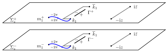
Figure 7. The oriented cut $[m_{1},k_{1}]^{-}\cup[k_{1},m_{1}]^{+}$ from the double pole $m_{1}^{-}$ on the lower sheet to the double zero $m_{1}^{+}$ on the upper sheet of $\Sigma_{z}$.

Proposition 6.2.

The complex-valued function $\psi(z,\cdot)$ has the following properties:

• $\psi(z,k)$ is analytic for $k\in\hat{\mathbb{C}}\backslash(\Gamma\cup[k_{1},m_{1}])$.

• Across $\Gamma$, $\psi(z,k)$ satisfies the jump relation

  $$\psi_{-}(z,k)=\psi_{+}(z,k)+\frac{2}{y(z,k^{+})}\log\left(\frac{\sqrt{w^{2}-1}-w}{\sqrt{w^{2}-1}+w}(k^{+})\right),\quad k\in\Gamma.$$ (6.20)

• Across the oriented straight-line segment $[k_{1},m_{1}]$, $\psi(z,k)$ satisfies the jump relation

  $$\psi_{-}(z,k)=\psi_{+}(z,k)+\frac{4\pi i}{y(z,k^{+})},\quad k\in[k_{1},m_{1}],$$ (6.21)

  where $k^{+}$ is the point in the upper sheet of $\Sigma_{z}$ which projects onto $k$, and $\psi_{-}(z,k)$ and $\psi_{+}(z,k)$ denote the values of $\psi$ on the left and right sides of $[k_{1},m_{1}]$.

• As $k\to m_{1}$,

  $$\psi(z,k)\to\frac{2}{y(z,k^{+})}\log(k-m_{1}).$$ (6.22)

• As $k\to\infty$,

  $$\psi(z,k)=\frac{2\log f}{k^{2}}+O(k^{-3}).$$ (6.23)

• As $k\to k_{1}$,

  $$\psi(z,k)\to\frac{2\pi i}{y},$$ (6.24)

  where $y=y(z,k^{+})$ for $k^{+}$ just to the left of the cut $[k_{1},m_{1}^{+}]$ on $\Sigma_{z}^{+}$, and is analytically continued around the endpoint $k_{1}$ so that it equals $y(z,k^{-})$ when $k^{-}$ lies just to the left of the cut $[m_{1}^{-},k_{1}]$ on $\Sigma_{z}^{-}$.

Proof.

The analyticity of $\psi$ for $k\in\hat{\mathbb{C}}\backslash(\Gamma\cup[k_{1},m_{1}])$ follows from the definitions of $y(z,k)$ and $H(z,k)$. It follows from (6.3), (6.6), the fact that $\mathrm{tr}\,(\mathcal{Q}\mathcal{L})=0$, and tedious calculations that

$$\mathcal{L}_{21+}=(1-2w^{2})\mathcal{L}_{21-}+2w\hat{\mathcal{L}}_{22-},\quad\hat{\mathcal{L}}_{22+}=2w(w^{2}-1)\mathcal{L}_{21-}+(1-2w^{2})\hat{\mathcal{L}}_{22-},$$

for $k\in\Gamma^{+}$. Hence the jump of $H(z,k)$ across $\Gamma^{+}$ is given by

$$H_{-}(z,k)=H_{+}(z,k)\left(\frac{\sqrt{w^{2}-1}-w}{\sqrt{w^{2}-1}+w}\right)^{2},\quad k\in\Gamma^{+},$$ (6.25)

which gives (6.20). The jump (6.21) follows from (6.16). The asymptotic behavior (6.22) is a consequence of the fact $H(z,k)$ has a double zero at $k=m_{1}^{+}$. Equation (6.23) follows from (6.18) and the fact that $y(z,k^{+})=k^{2}+O(k)$ as $k\to\infty$. The behavior of $\psi$ as $k\to k_{1}$ follows from (6.14) and (6.16). ∎

6.4. Solution of the scalar RH problem

Using the Sokhotski-Plemelj formula, we find that the solution of the scalar RH problem presented in Proposition 6.2 is given by

$$\psi(z,k)= \;\frac{1}{\pi i}\int_{\Gamma}\frac{\mathrm{d}k^{\prime}}{y(z,k^{+\prime})(k^{\prime}-k)}\log\left(\frac{\sqrt{w^{2}-1}-w}{\sqrt{w^{2}-1}+w}(k^{+\prime})\right)$$

$$+2\int_{[k_{1},m_{1}]}\frac{\mathrm{d}k^{\prime}}{y(z,k^{\prime+})(k^{\prime}-k)}.$$ (6.26)

This can be rewritten in terms of contour integrals on $\Sigma_{z}$ as

$$\psi(z,k) =2\int_{\Gamma^{+}}\frac{h(k^{\prime})\mathrm{d}k^{\prime}}{y(z,k^{\prime})(k^{\prime}-k)}-2\int_{k_{1}}^{{}^{\prime}m^{-}_{1}}\frac{\mathrm{d}k^{\prime}}{y(z,k^{\prime})(k^{\prime}-k)},$$ (6.27)

where $h(k)$ is given by

$$h(k)=\frac{1}{2\pi i}\log\left(\frac{\sqrt{w^{2}(k)-1}-w(k)}{\sqrt{w^{2}(k)-1}+w(k)}\right),\qquad k\in\Gamma^{+},$$

and the prime on the integral from $k_{1}$ to $m_{1}^{-}$ indicates that the path of integration does not necessarily lie in the complement of the cut basis $\{a,b\}$. Since $w(k)=-2ik\Omega$, $h(k)$ can be written as in (3.1). Letting $k\to\infty$ in (6.27) and recalling (6.23), we obtain

$$\log f =\int_{k_{1}}^{{}^{\prime}m^{-}_{1}}\frac{k\mathrm{d}k}{y}-\int_{\Gamma^{+}}h(k)\frac{k\mathrm{d}k}{y},$$ (6.28a)

$$\int_{k_{1}}^{{}^{\prime}m^{-}_{1}}\frac{\mathrm{d}k}{y} =\int_{\Gamma^{+}}h(k)\frac{\mathrm{d}k}{y}.$$ (6.28b)

7. Theta functions

In this section, we derive the expressions for $f$, $e^{2U}$, and $a$ given in (3.3) and (3.4).

We define the map $\phi:\Sigma_{z}\to\mathbb{C}$ by

$$\phi(k)\equiv\phi(z,k)=\int_{-iz}^{k}\omega,\quad k\in\Sigma_{z},$$

where it is assumed that the integration contour lies within the fundamental polygon determined by $\{a,b\}$. The Jacobian variety $\text{Jac}(\Sigma_{z})$ of $\Sigma_{z}$ is defined by $\text{Jac}(\Sigma_{z})=\mathbb{C}/\mathbb{L}$, where $\mathbb{L}$ denotes the discrete lattice generated by $1$ and $B$. The composition of $\phi$ with the projection $\mathbb{C}\to\text{Jac}(\Sigma_{z})$ is the Abel map with base point $-iz$, and $\phi(k_{1})\in\mathbb{C}$ projects to the vector of Riemann constants in $\text{Jac}(\Sigma_{z})$, see [5, Chap. VII].

7.1. Proof of expression (3.3) for $f$

We first suppose that the contour from $k_{1}$ to $m_{1}^{-}$ in (6.28) lies in the fundamental polygon determined by $\{a,b\}$. Utilizing (3.2), (2.12), and (2.14) in (6.28), we deduce that

$$u=\int_{k_{1}}^{m_{1}^{-}}\omega,\quad f=e^{-\int_{k_{1}}^{m_{1}^{-}}\omega_{\infty^{+}\infty^{-}}+I}.$$ (7.1)

In view of the properties of zero divisors of theta functions (see [5, Thm. VI.3.1]) and the following symmetry properties for Abelian differentials (see [5, Chap. III])

$$\int_{b}\omega_{PQ}=2\pi i\int_{Q}^{P}\omega,\quad\int^{P}_{Q}\omega_{\infty^{+}\infty^{-}}=\int^{\infty^{+}}_{\infty^{-}}\omega_{PQ},\quad P,Q\in\Sigma_{z},$$ (7.2)

we obtain

$$e^{-\int_{k_{1}}^{m_{1}^{-}}\omega_{\infty^{+}\infty^{-}}}=\frac{\Theta\left(\phi(\infty^{+})\right)\Theta\left(\phi(\infty^{-})-u\right)}{\Theta\left(\phi(\infty^{+})-u\right)\Theta\left(\phi(\infty^{-})\right)}.$$ (7.3)

Since $\phi(\infty^{+})=-\phi(\infty^{-})$ and the theta function $\Theta$ is even, we can rewrite (7.3) as

$$e^{-\int_{k_{1}}^{m_{1}^{-}}\omega_{\infty^{+}\infty^{-}}}=\frac{\Theta\left(u-\phi(\infty^{-})\right)}{\Theta\left(u+\phi(\infty^{-})\right)},$$

which together with (7.1) leads to (3.3). It is easy to see that the answer remains if invariant if the contour from $k_{1}$ to $m_{1}^{-}$ is replaced by a contour which does not lie in the fundamental polygon determined by $\{a,b\}$, cf. [11].

7.2. Proof of expressions (3.4) for $e^{2U}$ and $a$

Since $u\in i\mathbb{R}$ and $I\in\mathbb{R}$, the expression for $e^{2U}$ in (3.4) can be derived as in [11]. With the expression for $e^{2U}$ at hand, the expression for $a$ in (3.4) can be obtained by following the argument in [8, Sect. V].

8. The metric function $e^{2\kappa}$

One useful tool in the study of the Ernst equation (2.5) is the use of branch point condensation arguments [10]. In this section, we apply such arguments to derive the expression (3.6) for $e^{2\kappa}$. An analogous derivation was considered in [11]. However, in contrast to the situation in [11], our function $h(k)$ which determines the jump of the scalar RH problem for $\psi(z,k)$ does not vanish at the endpoints of $\Gamma$. This means that the condensation argument has to be modified.

8.1. Proof of expression (3.6) for $e^{2\kappa}$

Given an integer $g\geq 2$ and $g-1$ branch cuts $\{[E_{j},F_{j}]\}_{j=2}^{g}$, let $\hat{\Sigma}_{z}$ be the Riemann surface of genus $g$ defined by the equation

$$\hat{y}^{2}=(k-\xi)(k-\bar{\xi})(k-k_{1})(k-\bar{k}_{1})\prod_{j=2}^{g}(k-E_{j})(k-F_{j}),$$

where $\xi:=-iz$. We define a cut basis $\{\hat{a}_{j},\hat{b}_{j}\}_{j=1}^{g}$ on $\hat{\Sigma}_{z}$ as follows: $\hat{a}_{1}$ surrounds the cut $C_{k_{1}}$ and, for $j=2,\dots,g$, $\hat{a}_{j}$ surrounds the cut $[E_{j},F_{j}]$ in the counterclockwise direction; $\hat{b}_{j}$ enters the upper sheet on the right side of $[-iz,i\bar{z}]$ and exits again on the right side $C_{k_{1}}$ for $j=1$ and on the right side of $[E_{j},F_{j}]$ for $j=2,\dots,g$. Then $\{\hat{a}_{j},\hat{b}_{j}\}_{j=1}^{g}$ is a natural generalization of the basis $\{a,b\}$ on $\Sigma_{z}$. Let $\hat{\omega}=\{\hat{\omega}_{1},...,\hat{\omega}_{g}\}^{T}$ denote the canonical dual basis and let $\hat{\Theta}(\hat{\omega})\equiv\Theta(\hat{\omega}|\hat{B})$ be the associated theta function. Let $p,q\in\mathbb{C}^{q}$ be $z$-independent vectors which satisfy $\hat{B}p+q\in\mathbb{R}^{g}$. The theta function with characteristics $p,q\in\mathbb{R}^{g}$ is defined for $\hat{v}\in\mathbb{C}^{g}$ by

$$\hat{\Theta}\begin{bmatrix}p\\ q\end{bmatrix}(\hat{v})=\hat{\Theta}(\hat{v}+\hat{B}p+q)\exp\left(2\pi i\left(\frac{1}{2}p^{T}\hat{B}p+p^{T}(\hat{v}+q)\right)\right).$$

Then the function $\hat{f}(z)$ defined by

$$\hat{f}(z)=\frac{\hat{\Theta}\begin{bmatrix}p\\ q\end{bmatrix}\left(\int_{\xi}^{\infty^{+}}\hat{\omega}\right)}{\hat{\Theta}\begin{bmatrix}p\\ q\end{bmatrix}\left(\int_{\xi}^{\infty^{-}}\hat{\omega}\right)}$$ (8.1)

satisfies the Ernst equation (2.5) and the corresponding metric function $e^{2\kappa}$ is given by

$$e^{2\hat{\kappa}}=\hat{K}_{0}\frac{\hat{\Theta}\begin{bmatrix}p\\ q\end{bmatrix}(0)\hat{\Theta}\begin{bmatrix}p\\ q\end{bmatrix}\left(\int_{\xi}^{\bar{\xi}}\hat{\omega}\right)}{\hat{\Theta}(0)\hat{\Theta}\left(\int_{\xi}^{\bar{\xi}}\hat{\omega}\right)},$$ (8.2)

where $\hat{K}_{0}$ is a constant determined by the requirement that $e^{2\hat{\kappa}}=1$ on the rotation axis [10]. Our goal is to recover the Ernst potential (3.3) by letting the branch points $E_{j},F_{j}$ in (8.1) condense along the contour $\Gamma$ for an appropriate choice of the characteristics $p,q$. Then, by applying the same condensation to (8.2), we will obtain the expression (3.6) for $e^{2\kappa}$.

In order to handle the fact that $h(k)$ does not vanish at the endpoints of $\Gamma$, we define, for each integer $n\geq 1$, an extension $\Gamma_{n}$ of $\Gamma$ by $\Gamma_{n}=[-i\rho_{0}-\frac{i}{n},i\rho_{0}+\frac{i}{n}]$. We first let each branch cut $[E_{j},F_{j}]$ shrink to a point $\kappa_{j}\in\Gamma_{n}$. In this limit, we have

$$\left(\hat{\omega}_{1},\dots,\hat{\omega}_{g}\right) \rightarrow\big{(}\omega,\frac{1}{2\pi i}\omega_{\kappa_{2}^{+}\kappa_{2}^{-}},...,\frac{1}{2\pi i}\omega_{\kappa_{g}^{+}\kappa_{g}^{-}}\big{)};$$ (8.3a)

$$\hat{B}_{11} \to B;\quad\hat{B}_{1j}\to\int_{\kappa_{j}^{-}}^{\kappa_{j}^{+}}\omega,\quad j=2,...,g;$$ (8.3b)

$$\hat{B}_{ij} \to\frac{1}{2\pi i}\int_{\kappa_{j}^{-}}^{\kappa_{j}^{+}}\omega_{\kappa_{i}^{+}\kappa_{i}^{-}},\quad i\neq j,\quad i,j=2,...,g;$$ (8.3c)

$$\hat{B}_{jj} =\frac{1}{\pi i}\log|E_{j}-F_{j}|+O(1),\quad j=2,...,g.$$ (8.3d)

We then let the $\kappa_{j}$ condense along $\Gamma_{n}$ with the density determined by the measure

$$\mathrm{d}m_{n}(\kappa)=-\frac{1}{2}\frac{\mathrm{d}h_{n}}{\mathrm{d}\kappa}(\kappa)\mathrm{d}\kappa,\quad\kappa\in\Gamma_{n},$$ (8.4)

where $h_{n}:\Gamma_{n}\to\mathbb{C}$ is a sequence of smooth functions which vanish identically near the endpoints of $\Gamma_{n}$ and which converge pointwise to $h(k)$ on $\Gamma$ as $n\to\infty$. Choosing

$$p=(p_{1},p_{2},...,p_{g})=:(p_{1},\tilde{p})\in\mathbb{C}\times\mathbb{R}^{g-1},\quad q=(0,...,0)\in\mathbb{R}^{g},$$

where the vector $\tilde{p}\in\mathbb{R}^{g-1}$ is such that $\tilde{p}_{j}\in(0,\frac{1}{2})$, $j=2,...,g$, we find from (8.3) that, as the branch points condense along $\Gamma_{n}$,

$$\hat{\Theta}\!\begin{bmatrix}p\\ 0\end{bmatrix}\!\!\left(\int^{Q}_{P}\hat{\omega}\right)\to\Theta\!\begin{bmatrix}p_{1}\\ 0\end{bmatrix}\!\!\left(\int_{\Gamma_{n}}\mathrm{d}m_{n}(\kappa)\int_{\kappa^{-}}^{\kappa^{+}}\omega+\int^{Q}_{P}\omega\right)e^{\frac{L_{n}}{2}+\int_{\Gamma_{n}}\mathrm{d}m_{n}(\kappa)\int_{P}^{Q}\omega_{\kappa^{+}\kappa^{-}}},$$ (8.5)

where

$$L_{n} =\int_{\Gamma_{n}}\mathrm{d}m_{n}(\kappa_{1})\int_{\Gamma_{n}}^{\prime}\mathrm{d}m_{n}(\kappa_{2})\int^{\kappa_{2}^{+}}_{\kappa_{2}^{-}}\omega_{\kappa_{1}^{+}\kappa_{1}^{-}}(\kappa)$$

$$=\frac{1}{2}\int_{\Gamma_{n}}\mathrm{d}\kappa_{1}h_{n}(\kappa_{1})\int_{\Gamma_{n}}^{\prime}h_{n}(\kappa_{2})\frac{\partial\omega_{\kappa^{+}_{1}\kappa^{-}_{1}}}{\partial\kappa_{1}}(\kappa_{2}^{+}),$$ (8.6)

and the prime on the integral indicates that the contour $\Gamma_{n}$ should be deformed slightly so that the pole at $\kappa_{1}=\kappa_{2}$ is avoided. Integrating by parts and using (7.2), we obtain

$$\int_{\Gamma_{n}}dm_{n}(\kappa)\int_{\kappa^{-}}^{\kappa^{+}}\omega =\int_{\Gamma_{n}^{+}}h_{n}(\kappa)\omega(\kappa)=:u_{n},$$ (8.7)

$$\int_{\Gamma_{n}}\mathrm{d}m_{n}(\kappa)\int^{\infty^{+}}_{\infty^{-}}\omega_{\kappa^{+}\kappa^{-}} =\int_{\Gamma_{n}^{+}}h_{n}(\kappa)\omega_{\infty^{+}\infty^{-}}(\kappa)=:I_{n}.$$ (8.8)

Using (8.5)-(8.8) in (8.1), we conclude that the right-hand side of (8.1) converges to the following Ernst potential in the limit as the branch points condense along $\Gamma_{n}$:

$$f_{n}=\frac{\Theta\begin{bmatrix}p_{1}\\ 0\end{bmatrix}\left(u_{n}+\int^{\infty^{+}}_{\xi}\omega\right)}{\Theta\begin{bmatrix}p_{1}\\ 0\end{bmatrix}\left(u_{n}+\int^{\infty^{-}}_{\xi}\omega\right)}e^{I_{n}}.$$ (8.9)

Letting $p_{1}=0$ and taking $n\to\infty$ in (8.9), we recover the Ernst potential (3.3). We would like to take the same limit in the expression for the metric function $e^{2\kappa_{n}}$ associated with $f_{n}$. However, we first need to regularize the expression for $L_{n}$. We find from (2.14) that

$$\frac{\partial\omega_{\kappa_{1}^{+}\kappa_{1}^{-}}}{\partial\kappa_{1}}(\kappa_{2}^{+})=\frac{y^{\prime}(\kappa_{1}^{+})(\kappa_{2}-\kappa_{1})+y(\kappa_{1}^{+})}{(\kappa_{2}-\kappa_{1})^{2}y(\kappa_{2}^{+})}d\kappa_{2}-\bigg{(}\int_{a}\frac{y^{\prime}(\kappa_{1}^{+})(\kappa-\kappa_{1})+y(\kappa_{1}^{+})}{(\kappa-\kappa_{1})^{2}y(\kappa)}d\kappa\bigg{)}\omega(\kappa_{2}^{+}).$$

Hence we can rewrite (8.6) as

$$L_{n}=L_{n}^{reg}+L_{n}^{rem},$$ (8.10)

where the regularized term $L_{n}^{reg}$ is defined by

$$L_{n}^{reg}= \;\frac{1}{2}\int_{\Gamma_{n}}\mathrm{d}\kappa_{1}h_{n}(\kappa_{1})\int_{\Gamma_{n}}^{\prime}h_{n}(\kappa_{2})\bigg{(}\frac{\partial\omega_{\kappa^{+}_{1}\kappa^{-}_{1}}}{\partial\kappa_{1}}(\kappa_{2}^{+})-\frac{\mathrm{d}\kappa_{2}}{(\kappa_{2}-\kappa_{1})^{2}}\bigg{)}$$

$$= \;\frac{1}{2}\bigg{\{}\int_{\Gamma_{n}}d\kappa_{1}h_{n}(\kappa_{1})\int_{\Gamma_{n}}^{\prime}h_{n}(\kappa_{2})\bigg{(}\frac{y^{\prime}(\kappa_{1}^{+})(\kappa_{2}-\kappa_{1})+y(\kappa_{1}^{+})-y(\kappa_{2}^{+})}{(\kappa_{2}-\kappa_{1})^{2}y(\kappa_{2}^{+})}\bigg{)}d\kappa_{2}$$

$$-\bigg{(}\int_{\Gamma_{n}}d\kappa_{1}h_{n}(\kappa_{1})\int_{a}\frac{y^{\prime}(\kappa_{1}^{+})(\kappa-\kappa_{1})+y(\kappa_{1}^{+})}{(\kappa-\kappa_{1})^{2}y(\kappa)}d\kappa\bigg{)}\bigg{(}\int_{\Gamma_{n}}h_{n}(\kappa_{2})\omega(\kappa_{2}^{+})\bigg{)}\bigg{\}}$$

and the remainder $L_{n}^{rem}$ is given by

$$L_{n}^{rem}=\frac{1}{2}\int_{\Gamma_{n}}d\kappa_{1}h_{n}(\kappa_{1})\int_{\Gamma_{n}}^{\prime}h_{n}(\kappa_{2})\frac{d\kappa_{2}}{(\kappa_{2}-\kappa_{1})^{2}}.$$

We have arranged the definition of $L_{n}^{reg}$ so that the integrand only has a simple pole at $\kappa_{2}=\kappa_{1}$. It follows that $L_{n}^{reg}$ has the well-defined limit $L^{reg}$ defined in (3.8) as $n\to\infty$. The key point is that the first double integral in (3.8) converges at the endpoints of $\Gamma$ despite the fact that $h$ is nonzero at these endpoints. The term $L_{n}^{rem}$, on the other hand, diverges as $n\to\infty$ due to ever growing contributions from the endpoints of $\Gamma$. However, since $L_{n}^{rem}$ is independent of $z$, it can be absorbed into the coefficient $\hat{K}_{0}$.

Furthermore, there exists a constant $C$ such that

$$e^{-\int^{P}_{P_{0}}\omega_{\xi\bar{\xi}}}=C\sqrt{\frac{P-\bar{\xi}}{P-\xi}},\quad P\in\Sigma_{z},$$ (8.11)

because both sides have a simple pole at $\xi$, a simple zero at $\bar{\xi}$, and are analytic elsewhere on $\Sigma_{z}$. Hence,

$$\int_{\xi}^{\bar{\xi}}\omega_{\kappa^{+}\kappa^{-}}=-\int_{\kappa^{-}}^{\kappa^{+}}\omega_{\xi\bar{\xi}}=\left[\log\sqrt{\frac{P-\bar{\xi}}{P-\xi}}\right]_{\kappa^{-}}^{\kappa^{+}}\in\pi i+2\pi i\mathbb{Z}.$$ (8.12)

Consequently, the second term in the exponent in (8.5) is independent of $z$ and can also be absorbed into the coefficient $\hat{K}_{0}$.

The above absorptions can be carried out by defining a new constant $K_{0n}$ by

$$K_{0n}=\hat{K}_{0}e^{L_{n}^{rem}+\int_{\Gamma_{n}}\mathrm{d}m_{n}(\kappa)\int_{\xi}^{\bar{\xi}}\omega_{\kappa^{+}\kappa^{-}}}.$$ (8.13)

As the branch points condense, we have $\hat{\Theta}(v)\to\Theta(v_{1})$ for each $v\in\mathbb{C}^{g}$, where $v_{1}$ denotes the first component of the vector $v\in\mathbb{C}^{g}$. Using this fact together with (8.5), (8.10), and (8.13) to compute the limit of (8.2) as the branch points condense along $\Gamma_{n}$, we see that the metric function $e^{2\kappa_{n}}$ corresponding to the Ernst potential $f_{n}$ can be expressed by

$$e^{2\kappa_{n}}=K_{0n}\frac{\Theta\!\begin{bmatrix}p_{1}\\ 0\end{bmatrix}\!\!\left(u_{n}\right)\!\Theta\!\begin{bmatrix}p_{1}\\ 0\end{bmatrix}\!\!\left(u_{n}+\int_{\xi}^{\bar{\xi}}\omega\right)}{\Theta(0)\Theta\left(\int_{\xi}^{\bar{\xi}}\omega\right)}e^{L_{n}^{reg}}.$$ (8.14)

We can now let $p_{1}=0$ and take the limit $n\to\infty$ in (8.9) and (8.14). Then $f_{n}$ converges to the solution (3.3) of the BVP (2.8), and $e^{2\kappa_{n}}$ converges to the associated metric function $e^{2\kappa}$ given by

$$e^{2\kappa}=K_{0}\frac{\Theta\left(u\right)\!\Theta\left(u+\int_{\xi}^{\bar{\xi}}\omega\right)}{\Theta(0)\Theta\left(\int_{\xi}^{\bar{\xi}}\omega\right)}e^{L^{reg}},$$ (8.15)

where $K_{0}$ is a $z$-independent constant. This completes the proof of the expression (3.6) for $e^{2\kappa}$; the explicit expression (3.7) for the constant $K_{0}$ will be derived in Section 9.

9. Solution near the rotation axis

In this section, we first complete the proof Theorem 3.6 by studying the asymptotic behavior of the Ernst potential and the metric functions near the rotation axis $\rho=0$. We then use these results to establish expressions for $a_{0}$ and $K_{0}$, thus completing also the proof of Theorem 3.1.

As $\rho\to 0$, the branch cut $[-iz,i\bar{z}]$ shrinks to a point and $\Sigma_{z}$ degenerates to the genus zero Riemann surface $\Sigma^{\prime}$ defined by (2.15). In order to study this degeneration, we introduce the axis-adapted cut basis $\{\tilde{a},\tilde{b}\}$ on $\Sigma_{z}$ by (see Figure 8)

$$\begin{pmatrix}\tilde{a}\\ \tilde{b}\end{pmatrix}=\begin{pmatrix}-1&0\\ 0&-1\end{pmatrix}\begin{pmatrix}a\\ b\end{pmatrix}.$$ (9.1)

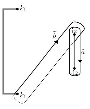
Figure 8. The axis-adapted basis $\{\tilde{a},\tilde{b}\}$ on $\Sigma_{z}$.

It then follows from the transformation formula for theta functions [6, Eq. (12)] that there exists a constant $c_{0}$ such that

$$\Theta(\tilde{{v}}|\tilde{B})=c_{0}\Theta(v|B),$$ (9.2)

where $\tilde{v}=-v$ and $\tilde{B}$ denotes the period matrix associated with $\{\tilde{a},\tilde{b}\}$. Let $\tilde{\omega}$ and $\tilde{u}$ denote the analogs of $\omega$ and $u$ in the axis-adapted basis $\{\tilde{a},\tilde{b}\}$ on $\Sigma_{z}$. Then

$$\tilde{\omega}=-\omega,\quad\tilde{u}=\int_{\Gamma^{+}}h\tilde{\omega}=-u.$$ (9.3)

It can also be verified by a residue computation that

$$\omega_{\infty^{+}\infty^{-}}=\tilde{\omega}_{\infty^{+}\infty^{-}}-2\pi i\tilde{\omega}$$

and consequently

$$I=\tilde{I}-2\pi i\tilde{u}\quad\text{where}\quad\tilde{I}=\int_{\Gamma^{+}}h\tilde{\omega}_{\infty^{+}\infty^{-}}.$$ (9.4)

Using the notation $\tilde{\Theta}(v)\equiv\Theta(v|\tilde{B})$, we can rewrite the expression (3.3) for the Ernst potential as

$$f(z)=\frac{\tilde{\Theta}(\tilde{u}-\int_{-iz}^{\infty^{-}}\tilde{\omega})}{\tilde{\Theta}(\tilde{u}+\int_{-iz}^{\infty^{-}}\tilde{\omega})}e^{\tilde{I}-2\pi i\tilde{u}}.$$ (9.5)

Define $c\equiv c(z)\in\mathbb{C}$, $J^{\prime}\equiv J^{\prime}(\zeta)\in\mathbb{R}$, and $K^{\prime}\equiv K^{\prime}(\zeta)\in\mathbb{C}$ by

$$c=\int^{\infty^{-}}_{k_{1}}\tilde{\omega},\quad J^{\prime}=\int_{\Gamma^{+}}h\omega^{\prime}_{\zeta^{+}\zeta^{-}},\quad K^{\prime}=\int_{k_{1}}^{\infty^{-}}\omega^{\prime}_{\zeta^{+}\zeta^{-}},$$

where $\omega^{\prime}_{PQ}$ denotes the Abelian differential of the third kind on $\Sigma^{\prime}$. Recalling the expression (2.16) for $\omega^{\prime}_{\zeta^{+}\zeta^{-}}$, we see that $J^{\prime}$ can be written as in (3.10).

Lemma 9.1.

We have $-e^{-K^{\prime}}=d$, where $d(\zeta)$ is the function in (3.10).

Proof.

A direct computation shows that

$$\frac{d}{dk}\log\bigg{(}\frac{\mu(k^{+})\mu(\zeta^{+})-\zeta k+k_{1}^{2}}{k-\zeta}\bigg{)}=\frac{\mu(\zeta^{+})}{(k-\zeta)\mu(k^{+})}.$$

Hence, using the expression (2.16) for $\omega^{\prime}_{\zeta^{+}\zeta^{-}}$,

$$K^{\prime} =-\mu(\zeta^{+})\int_{k_{1}}^{\infty}\frac{dk}{(k-\zeta)\mu(k^{+})}=-\log\bigg{(}\frac{\mu(k^{+})\mu(\zeta^{+})-\zeta k+k_{1}^{2}}{k-\zeta}\bigg{)}\bigg{|}_{k=k_{1}}^{\infty}$$

$$=-\log(\mu(\zeta^{+})-\zeta)+\log\bigg{(}\frac{-\zeta k_{1}+k_{1}^{2}}{k_{1}-\zeta}\bigg{)}=-\log\bigg{(}\frac{\mu(\zeta^{+})-\zeta}{k_{1}}\bigg{)},$$

which implies $e^{-K^{\prime}}=(\mu(\zeta^{+})-\zeta)/k_{1}=-d(\zeta)$. ∎

The following lemma gives the behavior of several quantities near the rotation axis.

Lemma 9.2.

Let $\zeta>0$. As $\rho\to 0$, it holds that

$$\tilde{u}=\frac{J^{\prime}}{2\pi i}+O(\rho^{2}), \tilde{\Theta}\bigg{(}\tilde{u}-\int_{-iz}^{\infty^{-}}\tilde{\omega}\bigg{)}=1-e^{J^{\prime}-K^{\prime}}+O(\rho^{2}),$$

$$c=\frac{K^{\prime}}{2\pi i}+O(\rho^{2}), \tilde{\Theta}\bigg{(}\tilde{u}+\int_{-iz}^{\infty^{-}}\tilde{\omega}\bigg{)}=1-e^{-J^{\prime}-K^{\prime}}+O(\rho^{2}),$$

$$\tilde{\Theta}\bigg{(}\tilde{u}+\int_{-iz}^{i\bar{z}}\tilde{\omega}\bigg{)}=1+\beta\rho+O(\rho^{2}), \tilde{\Theta}\bigg{(}\tilde{u}+\int_{i\bar{z}}^{\infty^{-}}\tilde{\omega}\bigg{)}=1+e^{-J^{\prime}-K^{\prime}}+O(\rho^{2}),$$

$$\tilde{\Theta}(\tilde{u})=1-\beta\rho+O(\rho^{2}), \tilde{\Theta}\bigg{(}\tilde{u}+\int_{-iz}^{\infty^{-}}\tilde{\omega}+\int_{i\bar{z}}^{\infty^{-}}\tilde{\omega}\bigg{)}=-\frac{e^{-J^{\prime}-2K^{\prime}-M^{\prime}}}{\rho}+O(1),$$ (9.6)

and

$$Q(u)=1-e^{-2J^{\prime}-2K^{\prime}}+O(\rho^{2}),\quad\tilde{I}=O(\rho^{2}),$$ (9.7)

where $\beta\in\mathbb{C}$ is a constant and $M^{\prime}$ is defined by

$$M^{\prime}=\frac{1}{2}\lim_{\epsilon\to 0}\left(\int^{(\zeta-\epsilon)^{+}}_{(\zeta-\epsilon)^{-}}\omega^{\prime}_{\zeta^{+}\zeta^{-}}-2\log\epsilon-2\log 2-\pi i\right).$$

The expansions in (9.6) and (9.7) remain valid if $\tilde{u}$ and $J^{\prime}$ are replaced by $0$ in all places.

Proof.

According to [6, Chap. III], $\tilde{\omega}$ and $\tilde{B}$ admit the following expansions as $\rho\to 0$:

$$\tilde{\omega}=\frac{1}{2\pi i}\omega^{\prime}_{\zeta^{+}\zeta^{-}}+O(\rho^{2}),\quad\tilde{B}=\frac{1}{\pi i}\log\rho+\frac{M^{\prime}}{\pi i}+O(\rho^{2}).$$ (9.8)

The expansions of $\tilde{u}$ and $c$ follow directly from (9.8) and the definitions. Moreover, note that

$$\int^{\infty^{-}}_{-iz}\tilde{\omega}=c+\frac{\tilde{B}}{2}-\frac{1}{2},\quad\int_{i\bar{z}}^{\infty^{-}}\tilde{\omega}=c+\frac{\tilde{B}}{2}.$$ (9.9)

By using (9.8), (9.9), and the expansions of $\tilde{u}$ and $c$, we get

$$\tilde{\Theta}\bigg{(}\tilde{u}-\int_{-iz}^{\infty^{-}}\tilde{\omega}\bigg{)}=\sum_{N\in\{0,1\}}e^{2\pi i(\frac{1}{2}\tilde{B}N(N-1)+N(\tilde{u}-c+\frac{1}{2}))}+O(\rho^{2})=1-e^{J^{\prime}-K^{\prime}}+O(\rho^{2}).$$

This establishes the expansion of $\tilde{\Theta}(\tilde{u}-\int_{-iz}^{\infty^{-}}\tilde{\omega})$; the other expansions in (9.6) are proved in a similar way. Note that (9.2) implies that $Q(u)$ is invariant under the change of basis $\{a,b\}\rightarrow\{\tilde{a},\tilde{b}\}$. The asymptotic behavior of $Q(u)$ then follows by substituting the expansions in (9.6) into (3.5). Finally, we have $\tilde{I}=I^{\prime}+O(\rho^{2})$ where $I^{\prime}=\int_{\Gamma^{+}}h\omega^{\prime}_{\infty^{+}\infty^{-}}$. But $I^{\prime}=0$ because $h(k)$ is an odd function of $k$. This proves (9.7). ∎

Proof of Theorem 3.6..

In view of Lemma 9.2, the behavior (3.11) of $f$ near the rotation axis follows from (9.4) and (9.5). The asymptotics (3.13) of $e^{2U}$ follows from Lemma 9.2 and the identity $e^{2U(z)}=Q(0)e^{I}/Q(u)$. These computations lead to the expressions

$$f(i\zeta)=\frac{1-e^{J^{\prime}-K^{\prime}}}{1-e^{-J^{\prime}-K^{\prime}}}e^{-J^{\prime}},\quad e^{2U(i\zeta)}=\frac{1-e^{-2K^{\prime}}}{1-e^{-2J^{\prime}-2K^{\prime}}}e^{-J^{\prime}},$$ (9.10)

for $f(i\zeta)$ and $e^{2U(i\zeta)}$. Using Lemma 9.1, we see that the expressions in (9.10) are consistent with the expressions (3.12) and (3.14) obtained in Section 5.

The fact that $a=O(\rho^{2})$ as $\rho\to 0$ is a consequence of (2.4), (3.4), and Lemma 9.2. Similarly, in view of (2.7) and (3.6), it is clear that $e^{2\kappa}-1=O(\rho^{2})$. This completes the proof of Theorem 3.6. ∎

Proof of the expressions for $a_{0}$ and $K_{0}$.

Expressing (3.4) in the axis-adapted basis $\{\tilde{a},\tilde{b}\}$ and letting $\rho\to 0$ in the resulting equation, we find

$$a_{0}=\lim_{\rho\to 0}\frac{\rho}{Q(0)^{2}}\frac{\tilde{\Theta}(\tilde{u}+\int_{-iz}^{\infty^{-}}\tilde{\omega}+\int_{i\bar{z}}^{\infty^{-}}\tilde{\omega})}{\tilde{\Theta}(\tilde{u}+\int_{-iz}^{i\bar{z}}\tilde{\omega})}e^{2\pi i\tilde{u}-\tilde{I}}.$$

Using Lemma 9.2 we conclude that

$$a_{0}=-\frac{e^{-2K^{\prime}-M^{\prime}}}{(1-e^{-2K^{\prime}})^{2}}.$$

Letting $\zeta\to\infty$ and using that $\lim_{\zeta\to\infty}e^{-2K^{\prime}}=0$ and

$$\lim_{\zeta\to\infty}(M^{\prime}+2K^{\prime})=\frac{1}{2}\lim_{R\to\infty}\left(-\int^{R^{+}}_{R^{-}}\omega^{\prime}_{\infty^{+}\infty^{-}}-2\log R-2\log 2-\pi i\right),$$

we infer that

$$a_{0}=-2\mathrm{i}\lim_{R\to\infty}R\exp\left(\int_{k_{1}}^{R^{+}}\omega^{\prime}_{\infty^{+}\infty^{-}}\right)=-2i\lim_{R\to\infty}Re^{-\int_{k_{1}}^{R}\frac{dk}{\mu(k^{+})}}.$$

Since

$$\frac{d}{dk}\log\big{(}k+\mu(k^{+})\big{)}=\frac{1}{\mu(k^{+})},$$

we obtain the sought-after expression for $a_{0}$:

$$a_{0} =-2i\lim_{R\to\infty}Re^{-\log(k+\mu(k^{+}))\big{|}_{k_{1}}^{R}}=-2i\lim_{R\to\infty}Re^{-\log(R+\sqrt{R^{2}+\frac{1}{4\Omega^{2}}})+\log k_{1}}=-\frac{1}{2\Omega}.$$

Writing the expression (3.6) for $e^{2\kappa}$ in terms of the axis-adapted basis $\{\tilde{a},\tilde{b}\}$, we get

$$e^{2\kappa}=K_{0}\frac{\tilde{\Theta}\left(\tilde{u}\right)\tilde{\Theta}\left(\tilde{u}+\int^{i\bar{z}}_{-iz}\tilde{\omega}\right)}{\tilde{\Theta}\left(0\right)\tilde{\Theta}\left(\int^{i\bar{z}}_{-iz}\tilde{\omega}\right)}e^{\frac{1}{2}\int_{\Gamma}^{\prime}\mathrm{d}\kappa_{1}h(\kappa_{1})\int_{\Gamma}h(\kappa_{2})\big{(}\frac{\partial\tilde{\omega}_{\kappa^{+}_{1}\kappa^{-}_{1}}}{\partial\kappa_{1}}(\kappa_{2}^{+})-\frac{\mathrm{d}\kappa_{2}}{(\kappa_{2}-\kappa_{1})^{2}}\big{)}}.$$

The expression (3.7) for $K_{0}$ follows by letting $\rho\to 0$ and using that $e^{2\kappa}=1$ on the rotation axis. This completes the proof of the formulas for $a_{0}$ and $K_{0}$ and thus also of Theorem 3.1. ∎

References

- [1] M. Bardeen and R. V. Wagoner, Uniformly rotating disks in general relativity, Astrophys. J., 158 (1969), pp. L65–L69.
- [2] , Relativistic disks. I. Uniform rotation, Astrophys. J., 167 (1971), pp. 359–423.
- [3] J. r. Bičák, Selected solutions of Einstein’s field equations: Their role in general relativity and astrophysics, in Einstein’s field equations and their physical implications, vol. 540 of Lecture Notes in Phys., Springer, Berlin, 2000, pp. 1–126.
- [4] F. J. Ernst, New formulation of the axially symmetric gravitational field problem, Phys. Rev., 167 (1968), pp. 1175–1178.
- [5] H. M. Farkas and I. Kra, Riemann Surfaces, Springer, 1992.
- [6] J. D. Fay, Theta Functions on Riemann Surfaces, vol. 352, Springer, 2006.
- [7] A. S. Fokas, A unified transform method for solving linear and certain nonlinear PDEs, Proc. Roy. Soc. Lond. A 453 (1997), pp. 1411–1443.
- [8] C. Klein and O. Richter, Physically realistic solutions to the Ernst equation on hyperelliptic Riemann surfaces, Phys. Rev. D, 58 (1998), p. 124018.
- [9] C. Klein and O. Richter, Ernst Equation and Riemann Surfaces: Analytical and Numerical Methods, vol. 685, Springer Science & Business Media, 2005.
- [10] D. A. Korotkin and V. B. Matveev, Theta function solutions of the Schlesinger system and the Ernst equation, Funct. Anal. Appl., 34 (2000), pp. 252–264.
- [11] J. Lenells, Boundary value problems for the stationary axisymmetric Einstein equations: A disk rotating around a black hole, Comm. Math. Phys., 304 (2011), pp. 585–635.
- [12] J. Lenells and A. S. Fokas, Boundary-value problems for the stationary axisymmetric Einstein equations: a rotating disc, Nonlinearity, 24 (2011), pp. 177–206.
- [13] R. Meinel, M. Ansorg, A. Kleinwächter, G. Neugebauer, and D. Petroff, Relativistic Figures of Equilibrium, Cambridge University Press Cambridge (UK), 2008.
- [14] G. Neugebauer, Gravitostatics and rotating bodies, in General relativity (Aberdeen, 1995), Scott. Univ. Summer School Phys., Edinburgh, 1996, pp. 61–81.
- [15] G. Neugebauer and R. Meinel, The Einsteinian gravitational field of the rigidly rotating disk of dust, The Astrophys. J., 414 (1993), pp. L97–L99.
- [16] , General relativistic gravitational field of a rigidly rotating disk of dust: Axis potential, disk metric, and surface mass density, Phys. Rev. Lett., 73 (1994), p. 2166.
- [17] , General relativistic gravitational field of a rigidly rotating disk of dust: Solution in terms of ultraelliptic functions, Phys. Rev. Lett., 75 (1995), p. 3046.