Lepton Flavor Violation in a $Z^{\prime}$ model for the $b\to s$ anomalies

Abstract

In recent years, several observables associated to semileptonic $b\to s$ processes have been found to depart from their predicted values in the Standard Model, including a few tantalizing hints of lepton flavor universality violation. In this work we consider an existing model with a massive $Z^{\prime}$ boson that addresses the anomalies in $b\to s$ transitions and extend it with a non-trivial embedding of neutrino masses. We analyze lepton flavor violating effects, induced by the non-universal interaction associated to the $b\to s$ anomalies and by the new physics associated to the neutrino mass generation, and determine the expected ranges for the most relevant observables.

I Introduction

The Standard Model (SM) of particle physics provides a precise description to a vast amount of phenomena as well as a deep understanding of the fundamental laws that govern them. However, despite its outstanding success, it fails to accommodate several phenomenological issues that remain as central questions in current particle physics, such as the existence of non-zero neutrino masses. This is nowadays an undeniable experimental fact due to the measurements obtained by many neutrino oscillation experiments, which have led us to an increasingly accurate knowledge of the relevant parameters over the years deSalas:2017kay .

The scientific literature contains a myriad of SM extensions with new ingredients that generate neutrino masses. This includes models with Dirac Ma:2016mwh ; CentellesChulia:2018gwr or Majorana neutrinos Ma:1998dn , with neutrino masses induced at tree-level or radiatively Cai:2017jrq , at low- Boucenna:2014zba or high-energy scales, and by operators with low or high dimensionalities Anamiati:2018cuq . One of the most common signatures of these neutrino mass models is lepton flavor violation (LFV), which in many scenarios may lead to observable rates in processes involving charged leptons. This makes LFV a very important probe of neutrino mass models, and more generally of models with extended lepton sectors. See Calibbi:2017uvl for a recent review on LFV.

Rare decays stand among the most powerful tests of the SM. Interestingly, the LHCb collaboration has recently reported several deviations between the measurements and the SM predictions in observables associated to rare semileptonic B-meson decays involving a $b\to s$ quark flavor transition. These include several angular observables, the $P_{5}^{\prime}$ observable being the most popular one, as well as the branching ratios of several processes, most notably $B_{s}\to\phi\mu^{+}\mu^{-}$  Aaij:2015oid ; Aaij:2015esa . Also recently, the Belle collaboration presented an independent measurement of $P_{5}^{\prime}$, compatible with the results obtained by LHCb Abdesselam:2016llu ; Wehle:2016yoi . In addition, the LHCb collaboration has also measured the theoretically clean ratios

$$R_{K^{(\ast)}}=\frac{\int_{q^{2}_{\rm min}}^{q^{2}_{\rm max}}\frac{d\Gamma(B\rightarrow K^{(\ast)}\mu^{+}\mu^{-})}{dq^{2}}\,dq^{2}}{\int_{q^{2}_{\rm min}}^{q^{2}_{\rm max}}\frac{d\Gamma(B\rightarrow K^{(\ast)}e^{+}e^{-})}{dq^{2}}\,dq^{2}}\,,$$ (1)

obtained for specific dilepton invariant mass squared ranges $q^{2}\in[q^{2}_{\rm min},q^{2}_{\rm max}]$. In the SM, these ratios are expected to be approximately equal to one, due to the fact that the SM gauge bosons couple with the same strength to all three families of leptons. These observables are precisely constructed to test this feature of the SM, known as lepton flavor universality (LFU). It is therefore very remarkable that LHCb reported values significantly lower than one, in one $q^{2}$ bin of the $R_{K}$ ratio Aaij:2014ora , as well as in two $q^{2}$ bins of the $R_{K^{\ast}}$ ratio Aaij:2017vbb :

$$R_{K} =0.745^{+0.090}_{-0.074}\pm 0.036\,,\quad q^{2}\in[1,6]~{}\text{GeV}^{2}\,,$$

$$R_{K^{\ast}} =0.660^{+0.110}_{-0.070}\pm 0.024\,,\quad q^{2}\in[0.045,1.1]~{}\text{GeV}^{2}\,,$$

$$R_{K^{\ast}} =0.685^{+0.113}_{-0.069}\pm 0.047\,,\quad q^{2}\in[1.1,6.0]~{}\text{GeV}^{2}\,.$$ (2)

These measurements imply deviations from the SM expected values Descotes-Genon:2015uva ; Bordone:2016gaq at the $2.6\,\sigma$ level in the case of $R_{K}$, $2.2\,\sigma$ for $R_{K^{\ast}}$ in the low-$q^{2}$ region, and $2.4\,\sigma$ for $R_{K^{\ast}}$ in the central-$q^{2}$ region. Belle has also reported on the apparent violation of LFU in the related observables $Q_{4}$ and $Q_{5}$ Wehle:2016yoi . These observations and their potential New Physics (NP) implications have made the $b\to s$ anomalies a subject of great interest.

It has been pointed out that the violation of lepton flavor universality generically implies the violation of lepton flavor Glashow:2014iga . Although there are several explicit counterexamples to this rule Celis:2015ara ; Alonso:2015sja , this connection does indeed exist in most of the models introduced to explain the $b\to s$ anomalies. In fact, this connection may be used to learn about neutrino oscillation parameters Boucenna:2015raa . However, since many of these models do not account for the observed neutrino masses and mixings, one may question whether the most relevant LFV effects are generally induced by the non-universal interactions associated to the $b\to s$ anomalies or by the NP associated to the generation of neutrino masses. Furthermore, even if the explanation to the $b\to s$ anomalies also involves LFV, the resulting rates could perhaps be too low to be observed by the experiments taking place in the near future. It is the goal of this paper to address these questions in a particular model.

In this paper we consider a $Z^{\prime}$ model introduced to explain the $b\to s$ anomalies Sierra:2015fma , extended with a non-trival embedding of neutrino masses. As we will see below, the gauge structure required to explain the $b\to s$ anomalies restricts the model building for the generation of neutrino masses. Our focus will be on the phenomenological exploration of the resulting LFV signatures in this model, both at the usual low-energy experiments and in B-meson decays. This has been studied previously for generic $Z^{\prime}$ models in Crivellin:2015era ; Becirevic:2016zri .

The rest of the paper is organized as follows. In Sec. II we briefly review the current status of the $b\to s$ anomalies and establish some basic notation to be used along the paper. In Sec. III we introduce the model and discuss its most relevant features. Our setup for the phenomenological analysis as well as our results are described in detail in Sec. IV. Finally, we draw our conclusions in Sec. V.

II A brief review of the $\boldsymbol{b\to s}$ anomalies

In order to interpret the available data on $b\to s$ transitions it proves convenient to adopt an effective field theory language. The effective Hamiltonian for $b\to s$ transitions is

$$\mathcal{H}_{\text{eff}}=-\frac{4G_{F}}{\sqrt{2}}\,V_{tb}V_{ts}^{\ast}\,\frac{e^{2}}{16\pi^{2}}\,\sum_{k}\left(C_{k}\,\mathcal{O}_{k}+C^{\prime}_{k}\,\mathcal{O}^{\prime}_{k}\right)+\text{h.c.}\,.$$ (3)

Here $G_{F}$ is the Fermi constant, $e$ the electric charge and $V$ the Cabibbo-Kobayashi-Maskawa (CKM) matrix. $\mathcal{O}_{k}$ and $\mathcal{O}^{\prime}_{k}$ are the effective operators that contribute to $b\to s$ transitions, and $C_{k}$ and $C^{\prime}_{k}$ their Wilson coefficients. It is usually convenient to split the Wilson coefficients into the SM and the NP contributions, $C_{k}=C_{k}^{\text{SM}}+C_{k}^{\text{NP}}$. In the following we will indicate their leptonic flavor indices explicitly. The operators that will be relevant for our discussion are

$$\mathcal{O}_{9}^{\ell_{i}\ell_{j}}=\left(\bar{s}\gamma_{\mu}P_{L}b\right)\,\left(\bar{\ell}_{i}\gamma^{\mu}\ell_{j}\right)\quad,\quad\mathcal{O}_{10}^{\ell_{i}\ell_{j}}=\left(\bar{s}\gamma_{\mu}P_{L}b\right)\,\left(\bar{\ell}_{i}\gamma^{\mu}\gamma_{5}\ell_{j}\right)\,.$$ (4)

Primed operators are obtained by replacing $P_{L}$ by $P_{R}$ in the quark current and $\ell_{i,j}=e,\mu,\tau$ are the three lepton flavors. One can use data on $b\to s$ transitions to constrain the Wilson coefficients of these operators. Interestingly, several independent global fits Capdevila:2017bsm ; Altmannshofer:2017yso ; DAmico:2017mtc ; Hiller:2017bzc ; Geng:2017svp ; Ciuchini:2017mik ; Alok:2017sui ; Hurth:2017hxg have found that the tension between the SM predictions and the experimental results can be alleviated with the introduction of a negative NP contribution in $C_{9}^{\mu\mu}$, leading to a total Wilson coefficient significantly smaller than the one in the SM. This has driven a general interest in the $b\to s$ anomalies resulting in many NP models aiming at an explanation of the experimental observations.

III The model

We consider an extended version of the model introduced in Sierra:2015fma that also accounts for the existence of non-zero neutrino masses. A sketch of this version of the model was presented in Sec. III.B of Sierra:2015fma .

The gauge group of the model is $\mathrm{SU(3)_{c}}\times\mathrm{SU(2)_{L}}\times\mathrm{U(1)_{Y}}\times\mathrm{U(1)_{X}}$, hence extending the SM gauge symmetry with an additional $\mathrm{U(1)_{X}}$ factor. The gauge coupling associated to this symmetry will be denoted by $g_{X}$ and the gauge boson by $Z^{\prime}$. Besides the usual SM fields, neutral under $\mathrm{U(1)_{X}}$, the matter content of the model is composed by one generation of vector-like (VL) quark doublets $Q_{L,R}=\left(U,D\right)_{L,R}$, two generations of vector-like lepton doublets $L_{L,R}=\left(N,E\right)_{L,R}$, the electroweak singlet scalars $\phi$ and $S$ and two generations of vector-like fermions $F$.  All new fields are charged under $\mathrm{U(1)_{X}}$. The complete scalar and fermion particle content of the model is given in Table 1.

	generations	$\mathrm{SU(3)}_{c}$	$\mathrm{SU(2)}_{L}$	$\mathrm{U(1)}_{Y}$	$\mathrm{U(1)}_{X}$
$H$	1	${\bf 1}$	${\bf 2}$	$1/2$	$0$
$\phi$	1	${\bf 1}$	${\bf 1}$	$0$	$2$
$S$	1	${\bf 1}$	${\bf 1}$	$0$	$-4$
$q_{L}$	3	${\bf 3}$	${\bf 2}$	$1/6$	$0$
$u_{R}$	3	${\bf 3}$	${\bf 1}$	$2/3$	$0$
$d_{R}$	3	${\bf 3}$	${\bf 1}$	$-1/3$	$0$
$\ell_{L}$	3	${\bf 1}$	${\bf 2}$	$-1/2$	$0$
$e_{R}$	3	${\bf 1}$	${\bf 1}$	$-1$	$0$
$Q_{L,R}$	1	${\bf 3}$	${\bf 2}$	$1/6$	$2$
$L_{L,R}$	2	${\bf 1}$	${\bf 2}$	$-1/2$	$2$
$F_{L,R}$	2	${\bf 1}$	${\bf 1}$	$0$	$2$

Table 1: Scalar and fermion particle content of the model.

The new Yukawa terms in the model are

$$-\mathcal{L}_{Y}=\lambda_{Q}\,\overline{Q_{R}}\,\phi\,q_{L}+\lambda_{L}\,\overline{L_{R}}\,\phi\,\ell_{L}+y\,\overline{L_{L}}\,H\,F_{R}+\widetilde{y}\,\overline{L_{R}}\,H\,F_{L}+h\,S\,\overline{F_{L}^{c}}\,F_{L}+\widetilde{h}\,S\,\overline{F_{R}^{c}}\,F_{R}+\,\text{h.c.}\,,$$ (5)

where $\lambda_{L}$ is a $2\times 3$ matrix, $y$ and $\widetilde{y}$ are $2\times 2$ matrices and $h$ and $\widetilde{h}$ are $2\times 2$ symmetric matrices. The $\lambda_{Q}$ and $\lambda_{L}$ couplings are the only ones involving the SM fermions, and thus play a crucial role in the resolution of the $b\to s$ anomalies. Furthermore, the vector-like fermions $Q$, $L$ and $F$ have gauge invariant Dirac mass terms

$$-\mathcal{L}_{m}=m_{Q}\,\overline{Q_{L}}Q_{R}+m_{L}\,\overline{L_{L}}L_{R}+m_{F}\,\overline{F_{L}}F_{R}+\text{h.c.}\,.$$ (6)

Both $m_{L}$ and $m_{F}$ are $2\times 2$ matrices. The scalar potential of the model can be split as

$$\mathcal{V}=\mathcal{V}_{\text{SM}}+\Delta\mathcal{V}\,.$$ (7)

Here $\displaystyle\mathcal{V}_{\text{SM}}=m_{H}^{2}|H|^{2}+\frac{\lambda}{2}|H|^{4}$ is the usual SM scalar potential. The new terms involving the $\mathrm{U(1)_{X}}$ charged scalars are

$$-\Delta\mathcal{V}= \,m_{\phi}^{2}\,|\phi|^{2}+m_{S}^{2}\,|S|^{2}+\frac{\lambda_{\phi}}{2}\,|\phi|^{4}+\frac{\lambda_{S}}{2}\,|S|^{4}$$

$$+\lambda_{H\phi}\,|H|^{2}|\phi|^{2}+\lambda_{HS}\,|H|^{2}|S|^{2}+\lambda_{\phi S}\,|\phi|^{2}|S|^{2}+\left(\mu^{\prime}\,\phi^{2}S+\text{h.c.}\right)\,.$$ (8)

We will assume that the minimization of the potential leads to non-zero vacuum expectation values (VEVs) for all scalars,

$$\langle H^{0}\rangle=\frac{v}{\sqrt{2}}\,,\qquad\langle\phi\rangle=\frac{v_{\phi}}{\sqrt{2}}\,,\qquad\langle S\rangle=\frac{v_{S}}{\sqrt{2}}\,.$$ (9)

Here $H^{0}$ is the neutral component of the SM Higgs doublet $H$. The $\phi$ and $S$ fields will be responsible for the spontaneous breaking of $\mathrm{U(1)_{X}}$, giving a mass to the $Z^{\prime}$,

$$m_{Z^{\prime}}^{2}=4g_{X}^{2}\left(v_{\phi}^{2}+4v_{S}^{2}\right)\,.$$ (10)

In addition, $v_{\phi}$ will induce mixings between the vector-like fermions and their SM counterparts thanks to the $\lambda_{Q}$ and $\lambda_{L}$ Yukawa interactions in Eq. (5). As we will show below, this mixing plays a crucial role in the phenomenology of the model.

III.1 Neutrino masses

The definition of a conserved lepton number is not possible if $S$ gets a non-zero VEV. Indeed, $\displaystyle\langle S\rangle=\frac{v_{S}}{\sqrt{2}}\neq 0$ breaks lepton number, leading to Majorana neutrino masses . In order to find an expression for the light neutrino masses, one must diagonalize the complete $11\times 11$ neutral fermion mass matrix. In the basis $\mathcal{N}=\{\nu_{L},N_{R}^{c},N_{L},F_{R}^{c},F_{L}\}$, this matrix takes the form

$$\mathcal{M}_{\mathcal{N}}=\left(\begin{array}[]{ccccccccccc}0&-\frac{1}{\sqrt{2}}v_{\phi}\lambda_{L}^{T}&0&0&0\\ -\frac{1}{\sqrt{2}}v_{\phi}\lambda_{L}&0&m_{L}^{T}&0&\frac{1}{\sqrt{2}}v\,\widetilde{y}\\ 0&m_{L}&0&-\frac{1}{\sqrt{2}}v\,y&0\\ 0&0&-\frac{1}{\sqrt{2}}v\,y^{T}&\sqrt{2}\,v_{S}\,\widetilde{h}&m_{F}^{T}\\ 0&\frac{1}{\sqrt{2}}v\,\widetilde{y}^{T}&0&m_{F}&\sqrt{2}\,v_{S}\,h\end{array}\right)\,.$$ (11)

The diagonalization of this matrix can be performed in seesaw approximation by assuming $v_{S}\,h,v_{S}\,\widetilde{h}\ll v\,y,v\,\widetilde{y},v_{\phi}\,\lambda_{L}\ll m_{L,F}$. Importantly, we note that in the absence of the Yukawa couplings $y$ and $h$, $\widetilde{y}$ and $\widetilde{h}$ would not contribute to the generation of neutrino masses at leading order, participating only at higher orders in perturbation theory. For this reason, we will take the simplifying assumption $\widetilde{y}=\widetilde{h}=0$ in the following. The resulting $3\times 3$ mass matrix for the light neutrinos is found to be

$$m_{\nu}\simeq\frac{v^{2}v_{\phi}^{2}v_{S}}{2\sqrt{2}}\,\lambda_{L}^{T}\,m_{L}^{-1}\,y\,m_{F}^{-1}\,h\,\left(m_{F}^{-1}\right)^{T}\,y^{T}\left(m_{L}^{-1}\right)^{T}\lambda_{L}\,,$$ (12)

where higher order terms in $h\ll 1$ have been neglected. A diagrammatic representation of the mechanism for neutrino mass generation in this model is shown in Fig. 1.

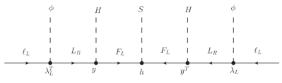
Figure 1: Neutrino mass generation. We note that the model under discussion provides a specific ultraviolet completion to the dimension-8 operator $\displaystyle\mathcal{O}_{\nu}=\frac{1}{\Lambda_{\nu}^{5}}\ell\ell HH\phi\phi S$ pointed out in Sierra:2015fma .

A neutrino mass matrix as the one in Eq. (12) formally resembles that obtained in the inverse seesaw Mohapatra:1986bd . Indeed, neutrino masses get suppresed due to the smallness of the $hv_{S}$ term, which allows for a low mass scale for the states that participate in the generation of neutrino masses. This justifies the choice $h\ll 1$, which is natural in the sense of ’t Hooft tHooft:1979rat , since the limit $h\to 0$ increases the symmetry of the model protecting this choice against quantum corrections. 

Given a specific texture for the $\lambda_{L}$ Yukawa matrices, one can always find a matrix $h$ that reproduces the observed neutrino masses and mixing angles. This matrix can be easily derived by inverting Eq. (12),

$$h=\bar{v}^{-5}\,m_{F}\,y^{-1}\,m_{L}\,\bar{\lambda}_{L}^{T}\,m_{\nu}\,\bar{\lambda}_{L}\,m_{L}^{T}\,\left(y^{-1}\right)^{T}\,m_{F}^{T}\,,$$ (13)

where $\bar{\lambda}_{L}$ is a $3\times 2$ matrix such that $\lambda_{L}\bar{\lambda}_{L}=\mathbb{I}_{2}$, $\mathbb{I}_{2}$ being the $2\times 2$ unit matrix, and we have defined $\displaystyle\bar{v}^{5}=\frac{v^{2}v_{\phi}^{2}v_{S}}{2\sqrt{2}}$. The neutrino mass matrix is diagonalized as

$$U^{T}\,m_{\nu}\,U=\widehat{m}_{\nu}\equiv\left(\begin{array}[]{ccc}m_{1}&0&0\\ 0&m_{2}&0\\ 0&0&m_{3}\end{array}\right)\,,$$ (14)

where

$$U=\left(\begin{array}[]{ccc}c_{12}c_{13}&s_{12}c_{13}&s_{13}e^{i\delta}\\ -s_{12}c_{23}-c_{12}s_{23}s_{13}e^{-i\delta}&c_{12}c_{23}-s_{12}s_{23}s_{13}e^{-i\delta}&s_{23}c_{13}\\ s_{12}s_{23}-c_{12}c_{23}s_{13}e^{-i\delta}&-c_{12}s_{23}-s_{12}c_{23}s_{13}e^{-i\delta}&c_{23}c_{13}\end{array}\right)$$ (15)

is the standard leptonic mixing matrix. Here $\delta$ is the CP-violating Dirac phase and we denote $c_{ij}=\cos\theta_{ij}$ and $s_{ij}=\sin\theta_{ij}$. 

III.2 Solving the $\boldsymbol{b\to s}$ anomalies

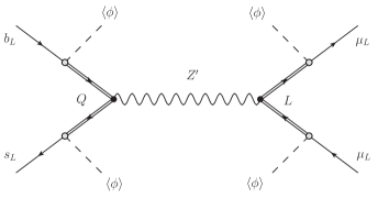
Figure 2: Generation of $\mathcal{O}_{9}$ and $\mathcal{O}_{10}$. The mixing between the SM fermions and the VL ones induce semileptonic four-fermion interactions.

The solution to the $b\to s$ anomalies follows the same lines as in Sierra:2015fma . The spontaneous breaking of the $\mathrm{U(1)_{X}}$ gauge symmetry by the $\phi$ VEV induces mixings between the SM and VL fermions due to the $\lambda_{Q}$ and $\lambda_{L}$ Yukawa couplings. Defining the bases $\mathcal{D}_{L,R}=\left\{d,D\right\}_{L,R}$ and $\mathcal{E}_{L,R}=\left\{e,E\right\}_{L,R}$, the Lagrangian after symmetry breaking includes the terms

$$-\mathcal{L}\supset\overline{\mathcal{D}_{L}}\mathcal{M}_{\mathcal{D}}\mathcal{D}_{R}+\overline{\mathcal{E}_{L}}\mathcal{M}_{\mathcal{E}}\mathcal{E}_{R}+\text{h.c.}\,.$$ (16)

The $4\times 4$ down-quark mass matrix is given by

$$\mathcal{M}_{\mathcal{D}}=\left(\begin{array}[]{cc}\frac{1}{\sqrt{2}}vY_{d}&\frac{1}{\sqrt{2}}v_{\phi}\lambda_{Q}^{T}\\ 0&-m_{Q}\end{array}\right)\,,$$ (17)

whereas the $5\times 5$ charged lepton mass matrix is

$$\mathcal{M}_{\mathcal{E}}=\left(\begin{array}[]{ccc}\frac{1}{\sqrt{2}}vY_{e}&\frac{1}{\sqrt{2}}v_{\phi}\lambda_{L}^{T}\\ 0&-m_{L}\end{array}\right)\,,$$ (18)

with the SM Yukawa couplings defined as $Y_{d}\,H\,\overline{q_{L}}\,d_{R}$ and $Y_{e}\,H\,\overline{\ell_{L}}\,e_{R}$. These two fermion mass matrices can be diagonalized by means of the following biunitary transformations

$$\mathcal{D}_{L}=V_{d}\,\widehat{\mathcal{D}_{L}}\,,\quad \quad\mathcal{D}_{R}=U_{d}\,\widehat{\mathcal{D}_{R}}\,,$$ (19)

$$\mathcal{E}_{L}=V_{e}\,\widehat{\mathcal{E}_{L}}\,,\quad \quad\mathcal{E}_{R}=U_{e}\,\widehat{\mathcal{E}_{R}}\,,$$ (20)

where $V_{d,e}$ and $U_{d,e}$ are unitary matrices and $\widehat{\mathcal{D}_{L,R}}$ and $\widehat{\mathcal{E}_{L,R}}$ denote the physical mass eigenstates. With these definitions, the diagonal mass matrices $\widehat{\mathcal{M}_{\mathcal{D}}}$ and $\widehat{\mathcal{M}_{\mathcal{E}}}$ are obtained as $\widehat{\mathcal{M}_{\mathcal{D}}}=V_{d}^{\dagger}\,\mathcal{M}_{\mathcal{D}}\,U_{d}$ and $\widehat{\mathcal{M}_{\mathcal{E}}}=V_{e}^{\dagger}\,\mathcal{M}_{\mathcal{E}}\,U_{e}$, respectively.

The SM-VL mixing leads to the generation of $Z^{\prime}$ effective couplings to the SM fermions. If these are parametrized as Buras:2012jb ; Altmannshofer:2014rta

$$\mathcal{L}\supset\bar{f}_{i}\gamma^{\mu}\left(\Delta_{L}^{f_{i}f_{j}}P_{L}+\Delta_{R}^{f_{i}f_{j}}P_{R}\right)f_{j}Z_{\mu}^{\prime}\,.$$ (21)

the $Z^{\prime}-b-s$ and $Z^{\prime}-\mu-\mu$ couplings, relevant for the explanation of the $b\to s$ anomalies, are given by

$$\Delta_{L}^{bs} =-2\,g_{X}\,\left(V_{d}\right)_{42}^{\ast}\,\left(V_{d}\right)_{43}\,,$$ (22)

$$\Delta_{L}^{\mu\mu} =-2\,g_{X}\,\sum_{k=4,5}\left(V_{e}\right)_{k2}^{\ast}\,\left(V_{e}\right)_{k2}\,.$$ (23)

These couplings lead to a tree-level contribution to the four-fermion operators $\mathcal{O}_{9}$ and $\mathcal{O}_{10}$, as shown in Fig. 2. In fact, since the SM fermions participating in the effective vertices are purely left-handed, the operators $\mathcal{O}_{9}$ and $\mathcal{O}_{10}$ are generated simultaneously, with their Wilson coefficients fulfilling Altmannshofer:2014rta

$$C_{9}^{\mu\mu,\text{NP}}=-C_{10}^{\mu\mu,\text{NP}}=-\frac{\Delta_{L}^{bs}\Delta_{L}^{\mu\mu}}{V_{tb}V_{ts}^{\ast}}\,\left(\frac{\Lambda_{v}}{m_{Z^{\prime}}}\right)^{2}\,,$$ (24)

where we have defined

$$\Lambda_{v}=\left(\frac{\pi}{\sqrt{2}G_{F}\alpha}\right)^{1/2}\simeq 4.94\,\text{TeV}\,,$$ (25)

with $\alpha=\frac{e^{2}}{4\pi}$ the electromagnetic fine structure constant. With these ingredients at hand, it is straightforward to check that the model under discussion can reproduce the required value for $C_{9}^{\mu\mu,\text{NP}}$ found by the global fits to $b\to s$ data. In our numerical analysis we will always consider parameter values that do so. Furthermore, analogous operators with violation of lepton flavor are also induced. Generalizing Eq. (23) to

$$\Delta_{L}^{\ell_{i}\ell_{j}}=-2\,g_{X}\,\sum_{k=4,5}\left(V_{e}\right)_{ki}^{\ast}\,\left(V_{e}\right)_{kj}\,,$$ (26)

one also has

$$C_{9}^{\ell_{i}\ell_{j},\text{NP}}=-\frac{\Delta_{L}^{bs}\Delta_{L}^{\ell_{i}\ell_{j}}}{V_{tb}V_{ts}^{\ast}}\,\left(\frac{\Lambda_{v}}{m_{Z^{\prime}}}\right)^{2}\,.$$ (27)

The $C_{9}^{\ell_{i}\ell_{j},\text{NP}}$ LFV Wilson coefficients are the source of the B-meson LFV decays discussed in this work.

III.3 Dark matter

Finally, we note that the setup described here can be minimally extended to account for the dark matter of the Universe. Indeed, the original model introduced in Sierra:2015fma was the first NP model addressing the $b\to s$ anomalies with a dark sector. This was accomplished by adding the complex scalar $\chi$, with charges $\left({\bf 1},{\bf 1},0,-1\right)$ under $\mathrm{SU(3)_{c}}\times\mathrm{SU(2)_{L}}\times\mathrm{U(1)_{Y}}\times\mathrm{U(1)_{X}}$. Assuming that this scalar does not get a VEV, the breaking of the $\mathrm{U(1)_{X}}$ gauge symmetry leaves a remnant $\mathbb{Z}_{2}$ parity, under which $\chi$ is odd. This mechanism Krauss:1988zc ; Petersen:2009ip ; Sierra:2014kua automatically stabilizes $\chi$ and makes it a valid dark matter candidate. Furthermore, the heavy $Z^{\prime}$ boson, crucial for the explanation of the $b\to s$ anomalies, serves as a portal between the SM and dark sectors. This establishes a non-trivial link between these two phenomenological directions in the model. We refer to Sierra:2015fma for a detailed discussion of the dark matter phenomenology of the model and to Vicente:2018xbv for a recent review on the possible connection between the $b\to s$ anomalies and the dark matter of the Universe.

IV Phenomenological analysis

Our phenomenological analysis uses the FlavorKit Porod:2014xia functionality of SARAH Staub:2008uz ; Staub:2009bi ; Staub:2010jh ; Staub:2012pb ; Staub:2013tta for the analytical computation of the purely leptonic LFV observables.  This allows us to automatically obtain complete analytical results for the LFV observables as well as robust numerical routines when this is used in combination with SPheno Porod:2003um ; Porod:2011nf . For the calculation of the $B$-meson LFV branching ratios we follow Crivellin:2015era .

Let us now explain our parameter choices. Without loss of generality, the matrices $m_{L}$ and $m_{F}$ will be taken to be diagonal. We will also further assume a diagonal form for the $y$ matrix. Regarding the fit to neutrino oscillation data, we will consider a specific structure for the $\lambda_{L}$ matrix with $\left(\lambda_{L}\right)_{i1}=0$, thus forcing the matrix $h$ to contain flavor-violating entries. The matrix $h$ will be obtained by using Eq. (13).  Finally, we make the choice $\left(\lambda_{Q}\right)_{1}=0$ in order to suppress the $Z^{\prime}$ couplings to 1st generation quarks.

In what concerns the parameter ranges explored in the following analysis, we must take into account constraints derived from direct searches at the Large Hadron Collider (LHC). These include searches for the vector-like fermions in the model, as well as for the heavy $Z^{\prime}$ boson that mediates the NP contributions to the flavor observables. Regarding the $Z^{\prime}$ boson, one may naively think that its production cross-section would be too low to be observable at the LHC due to our choice $\left(\lambda_{Q}\right)_{1}=0$. However, the $Z^{\prime}$ can indeed be produced in $pp$ collisions due to the non-vanishing heavy quark content in the protons. Due to the large couplings to muons required to explain the $b\to s$ anomalies, it is expected to decay mainly into $\mu^{+}\mu^{-}$ (and, optionally, $\tau^{+}\tau^{-}$ if the $\left(\lambda_{L}\right)_{i3}$ couplings take large values). ATLAS Aaboud:2017buh and CMS Sirunyan:2018exx have searched for a $Z^{\prime}$ boson in the dimuon channel but the resulting limits are not very stringent, allowing for $Z^{\prime}$ masses as low as $\sim 100$ GeV, see Xu:2018 for a recent analysis. Ditau searches are more sensitive and require $m_{Z^{\prime}}\gtrsim 1$ TeV unless the $Z^{\prime}$ has a very large decay width Faroughy:2016osc . However, in our setup the $Z^{\prime}\to\tau^{+}\tau^{-}$ branching ratio will never be dominant due to the large couplings to muons, and hence $m_{Z^{\prime}}\sim 1$ TeV will be perfectly allowed. The LHC collaborations have also searched for the vector-like fermions in the model, which provide complementary collider bounds. The vector-like quarks are colored particles and thus efficiently produced via QCD interactions at the LHC. This implies lower bounds on their mass slightly above the TeV scale Cacciapaglia:2018lld . Since our setup works with vector-like quark masses above this scale, the existing bounds can be easily satisfied. Finally, the vector-like leptons can also be searched for in multilepton final states. The current limits are weaker than those for vector-like quarks and allow for masses below the TeV Xu:2018 . These constraints will be taken into account in the numerical analysis that follows.

We now proceed to present the main numerical results of our analysis.

IV.1 BR($\boldsymbol{B\to K\tau\mu}$) vs BR($\boldsymbol{\tau\to 3\,\mu}$)

We first discuss the correlation between $\text{BR}(B\to K\tau\mu)$ and $\text{BR}(\tau\to 3\,\mu)$ and how it can be used to estimate an upper bound for $\text{BR}(B\to K\tau\mu)$.  Assuming that the dominant contributions are induced by the tree-level exchange of the $Z^{\prime}$ boson (see below for a discussion on this point), the branching ratios for the $B\to K\tau\mu$ and $\tau\to 3\,\mu$ decays can be written as Crivellin:2015era

$$\text{BR}(B\to K\tau\mu) =\text{BR}(B\to K\tau^{-}\mu^{+})+\text{BR}(B\to K\tau^{+}\mu^{-})=$$

$$=2\cdot 10^{-9}\,A_{K\tau\mu}\,\left|\frac{\Delta_{L}^{bs}\Delta_{L}^{\tau\mu}}{V_{tb}V_{ts}^{\ast}}\right|^{2}\left(\frac{\Lambda_{v}}{m_{Z^{\prime}}}\right)^{4}\,,$$ (28)

$$\text{BR}(\tau\to 3\,\mu) =\frac{m_{\tau}^{5}}{768\pi^{3}\Gamma_{\tau}m_{Z^{\prime}}^{4}}\left|\Delta_{L}^{\mu\mu}\Delta_{L}^{\tau\mu}\right|^{2}\,,$$ (29)

where $m_{\tau}$ and $\Gamma_{\tau}$ are the tau lepton mass and decay width, respectively, and $A_{K\tau\mu}=19.6\pm 1.7$. This parameter has been obtained by combining the coefficients $a_{K\tau\mu}+b_{K\tau\mu}$, see Crivellin:2015era , and adding the $a_{K\tau\mu}$ and $b_{K\tau\mu}$ errors in quadrature. We note that although Ref. Becirevic:2016zri provides slightly different numerical values for these coefficients, they are perfectly compatible, in particular given the level of precision required for our analysis. One can now combine these expressions with Eq. (24) to obtain

$$\frac{\text{BR}(B\to K\tau\mu)}{\text{BR}(\tau\to 3\,\mu)}=1.7\cdot 10^{7}\,\text{TeV}^{4}\left(\frac{\left|\Delta_{L}^{bs}\right|}{m_{Z^{\prime}}}\right)^{4}\,\frac{1}{\left|C_{9}^{\mu\mu,\text{NP}}\right|^{2}}\,.$$ (30)

The ratio $\left|\Delta_{L}^{bs}\right|/m_{Z^{\prime}}$ is strongly constrained by $B_{s}-\overline{B_{s}}$ mixing, which in this model would be induced via $Z^{\prime}$ tree-level exchange. Allowing for a $10\%$ deviation in the mixing amplitude, one finds Altmannshofer:2014rta  

$$\frac{m_{Z^{\prime}}}{\left|\Delta_{L}^{bs}\right|}\gtrsim 244\,\text{TeV}\quad\Rightarrow\quad\frac{\left|\Delta_{L}^{bs}\right|}{m_{Z^{\prime}}}\lesssim 4\cdot 10^{-3}\,\text{TeV}^{-1}\,.$$ (31)

Furthermore, the current experimental upper bound on $\text{BR}(\tau\to 3\,\mu)$ has been set by the Belle collaboration, which obtained $\text{BR}(\tau\to 3\,\mu)_{\text{max}}=2.1\times 10^{-8}$ Hayasaka:2010np , whereas the preferred $2\sigma$ range obtained for $C_{9}^{\mu\mu,\text{NP}}$ in the global fit Capdevila:2017bsm is $\left[-0.88,-0.37\right]$. With these ingredients at hand one can easily obtain the largest branching ratio for the $B\to K\tau\mu$ decay in this model, finding

$$\text{BR}(B\to K\tau\mu)_{\text{max}}\lesssim 8\cdot 10^{-10}\,.$$ (32)

This result is clearly below the current experimental limit, $\text{BR}(B\to K\tau\mu)<4.8\cdot 10^{-5}$ Amhis:2014hma . The main reason behind this result is the stringent constraint from $B_{s}-\overline{B_{s}}$ mixing. However, we would like to emphasize two points: (1) this is the largest $\text{BR}(B\to K\tau\mu)$ that one expects when the $Z^{\prime}$ boson has purely left-handed couplings, as in the model under consideration, and (2) while in models with additional $Z^{\prime}$ right-handed couplings cancellations in the $B_{s}-\overline{B_{s}}$ mixing amplitude are possible Crivellin:2015era , increasing $\text{BR}(B\to K\tau\mu)_{\text{max}}$ beyond the value given in Eq. (32) would require a significant fine-tuning of the parameters.

Figure 3 shows the correlation between $\text{BR}(B\to K\tau\mu)$ and $\text{BR}(\tau\to 3\,\mu)$ for three specific parameter choices. This figure has been obtained varying $\left(\lambda_{L}\right)_{13}=\left(\lambda_{L}\right)_{22}$. The values of the model parameters in the three different scenarios are:

• Green: $g_{X}=0.155$, $v_{S}=10.6$ GeV, $m_{Z^{\prime}}=1592$ GeV, $\left(m_{L}\right)_{11}=\left(m_{L}\right)_{22}=1904$ GeV and $\left(\lambda_{Q}\right)_{2}=\left(\lambda_{Q}\right)_{3}=0.0407$.

• Blue: $g_{X}=0.2$, $v_{S}=200$ GeV, $m_{Z^{\prime}}=1010$ GeV, $\left(m_{L}\right)_{11}=\left(m_{L}\right)_{22}=1600$ GeV, $\left(\lambda_{Q}\right)_{2}=\left(\lambda_{Q}\right)_{3}=0.055$.

• Purple: $g_{X}=0.4$, $v_{S}=34$ GeV, $m_{Z^{\prime}}=2330$ GeV, $\left(m_{L}\right)_{11}=\left(m_{L}\right)_{22}=1007$ GeV, $\left(\lambda_{Q}\right)_{2}=\left(\lambda_{Q}\right)_{3}=0.052$.

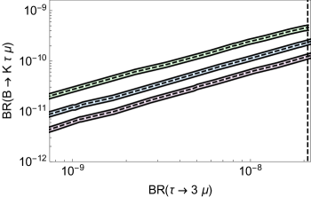
Figure 3: Correlation between BR($\tau\to 3\mu$) and BR($B\to K\tau\mu$) for three different sets of parameters. This figure has been obtained varying $\left(\lambda_{L}\right)_{13}=\left(\lambda_{L}\right)_{22}$. The vertical dashed line corresponds to the Belle experimental bound BR($\tau\to 3\,\mu$)${}_{\text{max}}=2.1\cdot 10^{-8}$ Hayasaka:2010np .

We note that higher values of $\left(\lambda_{Q}\right)_{2}=\left(\lambda_{Q}\right)_{3}$ would be excluded due to $B_{s}-\overline{B_{s}}$ mixing constraints. The green band in Fig. 3 reaches $\text{BR}(B\to K\tau\mu)\sim 6\cdot 10^{-10}$, close to the upper bound estimated in Eq. (32). As we will show next, the strong correlations found in our analysis can be broken by loop effects, hence affecting the general conclusions derived from our phenomenological exploration. For instance, in regions of parameter space where loop corrections cancel the tree-level results for $\text{BR}(\tau\to 3\,\mu)$, Eq. (30) would no longer hold and a larger $\text{BR}(B\to K\tau\mu)$ would be allowed. This would require a fine-tuning of the masses and mixings in the charged lepton sector.

IV.2 On the relevance of loop effects in BR($\boldsymbol{\tau\to 3\,\mu}$)

So far we have discussed tree-level predictions of the model. However, one may wonder whether loop corrections might alter the results presented above. We have addressed this issue in Fig. 4, where we show the ratio between the tree-level expression for BR($\tau\to 3\,\mu$) given in Eq. (29) and the complete numerical result including 1-loop contributions as returned by SPheno,

$$R_{\tau 3\mu}=\frac{\text{BR}(\tau\to 3\,\mu)_{\text{tree-level}}}{\text{BR}(\tau\to 3\,\mu)_{\text{1-loop}}}\,.$$ (33)

This plot has been obtained by randomly scanning in the following ranges:

$$0.05 < g_{X}<1.0$$

$$10\text{ GeV} < v_{S}<500\text{ GeV}$$

$$0.01 < \left(\lambda_{Q}\right)_{2}=\left(\lambda_{Q}\right)_{3}<0.1$$

$$0.8\text{ TeV} < \left(m_{L}\right)_{11}=\left(m_{L}\right)_{22}<2\text{ TeV}$$

$$1\text{ TeV} < m_{Z^{\prime}}<3\text{ TeV}$$

One can clearly see in Fig. 4 that while the tree-level expression in Eq. (29) and the complete numerical result including 1-loop corrections are actually very similar for low values of $g_{X}$, they can be very different for $g_{X}>0.4$.

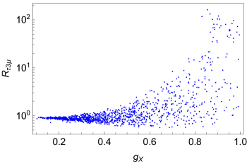
Figure 4: Behavior of the ratio $R_{\tau 3\mu}$ as a function of the gauge coupling $g_{X}$. Several model parameters have been randomly scanned over a wide range of numerical values, see text for details. The tree-level expression in Eq. (29) and the complete numerical result including 1-loop corrections can be very different for $g_{X}\gtrsim 0.4$.

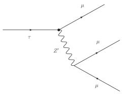
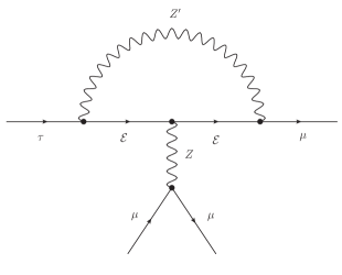
Figure 5: Feynman diagrams relevant for the calculation of the $\tau\to 3\,\mu$ amplitude. On the left, the dominant tree-level contribution is shown, whereas the diagram on the right is one of the dominant 1-loop contributions. We note that the 1-loop diagram on the right should be accompanied by two diagrams with the $Z$ boson line attached to one of the external lepton legs.

The impact of the loop corrections in $\tau\to 3\,\mu$ can be easily understood with the following considerations. In fact, it is not surprising that loop effects can be as large as the tree-level ones in $\tau\to 3\,\mu$. Fig. 5 shows two Feynman diagrams relevant for the calculation of the $\tau\to 3\,\mu$ amplitude. The diagram on the left constitutes the dominant tree-level contribution, whereas the diagram on the right is one of the dominant 1-loop contributions. Their contribution to the amplitude for external left-handed leptons can be generically written as

$$\mathcal{A}_{\rm tree} =\frac{g_{X}^{2}}{m_{Z^{\prime}}^{2}}\,F_{\rm tree}\left(V_{e}\right)\,,$$ (34)

$$\mathcal{A}_{\rm loop} =\frac{1}{16\pi^{2}}\,\frac{g_{X}^{2}\,g_{Z\ell\ell}}{m_{Z}^{2}}\,F_{\rm loop}^{g_{X}}\left(m_{\mathcal{E}},V_{e}\right)\,,$$ (35)

where $g_{Z\ell\ell}$ is the SM $Z$ boson coupling to a pair of left-handed charged leptons and $F_{\rm tree}$ and $F_{\rm loop}^{g_{X}}$ are two functions of the charged leptons (the five eigenstates) masses and mixings. $F_{\rm tree}$ only depends on the mixings in $V_{e}$ due the $Z^{\prime}$ couplings to $\tau\mu$ and $\mu\mu$, given in Eq. (26). In contrast, $F_{\rm loop}^{g_{X}}$ also depends on the five charged lepton masses, $m_{\mathcal{E}}$, due to the corresponding loop function. We first note that for $F_{\rm tree}\simeq F_{\rm loop}^{g_{X}}$, both contributions have comparable sizes, since

$$\frac{1}{16\pi^{2}}\,\frac{1}{m_{Z}^{2}}\sim\frac{1}{m_{Z^{\prime}}^{2}}\quad,\quad\text{for}\,m_{Z^{\prime}}\sim\text{TeV}\,.$$ (36)

Therefore, one would naively expect that loop effects in $\tau\to 3\,\mu$ will be generically of a size that is comparable to the tree-level ones. This is indeed what we find for large values of $g_{X}$. Moreover, we note that the 1-loop contributions may have a relative sign with respect to the tree-level ones, thus leading to cancellations in the final amplitudes, as shown in Fig. 4. In contrast, this is not the case for low values of $g_{X}$ ($g_{X}\lesssim 0.4$). In this region of the parameter space we find that $F_{\rm loop}^{g_{X}}$ is strongly reduced, hence suppressing loop contributions. This is due to the fact that, although $F_{\rm loop}^{g_{X}}$ does not depend explicitly on $g_{X}$, there is an indirect dependence on this gauge coupling. In order to keep $m_{Z^{\prime}}$ in the TeV ballpark for low values of $g_{X}$, one must introduce a large $v_{\phi}$ VEV, see Eq. (10), and this in turn affects the charged lepton masses and mixings as shown in Eq. (18). We have checked in detail that this is the reason behind the negligible loop effects for $g_{X}\lesssim 0.4$. However, we would like to point out that this behavior is not to be generally expected and emphasize the relevance of loop effects for a proper evaluation of BR($\tau\to 3\,\mu$) in $Z^{\prime}$ models for the $b\to s$ anomalies.

V Summary and conclusions

The hints reported by the LHCb collaboration may be the first indications of a completely unexpected New Physics sector with interactions that violate lepton flavor universality. In this paper we have explored an extension of the $Z^{\prime}$ model of Sierra:2015fma with a non-trivial embedding of neutrino masses and mixings. Our focus has been on the lepton flavor violating phenomenology of the resulting model, motivated by theoretical arguments that link it to the breaking of lepton flavor universality Glashow:2014iga .

The main conclusions of our phenomenological exploration can be summarized as follows:

• The additional degrees of freedom introduced to accommodate neutrino masses and mixings play a sub-dominant role in the lepton flavor violating predictions of the model, which are dominated by the New Physics effects induced by the states responsible for the explanation of the $b\to s$ anomalies.

• In most parts of the parameter space the rates for $B\to K\tau\mu$ and $\tau\to 3\,\mu$ are strongly correlated. This is simply due to the fact that both are dominated by tree-level $Z^{\prime}$ boson exchange. In this case, we have derived the upper limit $\text{BR}(B\to K\tau\mu)_{\text{max}}\lesssim 8\cdot 10^{-10}$. This limit applies to all models with purely left-handed $Z^{\prime}$ couplings and can only be evaded by fine-tuning the contributions to $B_{s}-\overline{B_{s}}$ mixing in models with both left- and right-handed $Z^{\prime}$ couplings Crivellin:2015era .

• Loop effects in $\tau\to 3\,\mu$ may be comparable to the tree-level ones. This is due to the strong suppression induced by the tree-level exchange of a TeV-scale $Z^{\prime}$ boson, which is absent in many 1-loop contributions. In fact, this feature is expected in generic $Z^{\prime}$ models for the $b\to s$ anomalies, although some regions of the parameter space of these models might deviate from this general expectation.

Flavor processes are clearly the most direct test of the model under discussion and crucial contributions from the Belle II experiment are expected in the long term Albrecht:2017odf . However, the model can also be probed in several complementary ways. Direct searches at the LHC can also provide an additional handle on the model. One can have observable production rates for the vector-like lepton in the model, see Xu:2018 for a recent work in this direction, or search for the mediator of the New Physics contributions, the heavy $Z^{\prime}$ boson, see for instance Faroughy:2016osc . If the $b\to s$ anomalies and the violation of flavor universality are finally confirmed, all these experimental approaches will be necessary to have a global picture of the new dynamics that lies beyond the Standard Model.

References

- (1) P. F. de Salas, D. V. Forero, C. A. Ternes, M. Tortola and J. W. F. Valle, Status of neutrino oscillations 2018: 3 hint for normal mass ordering and improved CP sensitivity, Phys. Lett. B782 (2018) 633–640, [1708.01186].
- (2) E. Ma and O. Popov, Pathways to Naturally Small Dirac Neutrino Masses, Phys. Lett. B764 (2017) 142–144, [1609.02538].
- (3) S. Centelles Chuliá, R. Srivastava and J. W. F. Valle, Seesaw roadmap to neutrino mass and dark matter, Phys. Lett. B781 (2018) 122–128, [1802.05722].
- (4) E. Ma, Pathways to naturally small neutrino masses, Phys. Rev. Lett. 81 (1998) 1171–1174, [hep-ph/9805219].
- (5) Y. Cai, J. Herrero-García, M. A. Schmidt, A. Vicente and R. R. Volkas, From the trees to the forest: a review of radiative neutrino mass models, Front.in Phys. 5 (2017) 63, [1706.08524].
- (6) S. M. Boucenna, S. Morisi and J. W. F. Valle, The low-scale approach to neutrino masses, Adv. High Energy Phys. 2014 (2014) 831598, [1404.3751].
- (7) G. Anamiati, O. Castillo-Felisola, R. M. Fonseca, J. C. Helo and M. Hirsch, High-dimensional neutrino masses, 1806.07264.
- (8) L. Calibbi and G. Signorelli, Charged Lepton Flavour Violation: An Experimental and Theoretical Introduction, Riv. Nuovo Cim. 41 (2018) 1, [1709.00294].
- (9) LHCb collaboration, R. Aaij et al., Angular analysis of the decay using 3 fb-1 of integrated luminosity, JHEP 02 (2016) 104, [1512.04442].
- (10) LHCb collaboration, R. Aaij et al., Angular analysis and differential branching fraction of the decay , JHEP 09 (2015) 179, [1506.08777].
- (11) Belle collaboration, A. Abdesselam et al., Angular analysis of , in Proceedings, LHCSki 2016 - A First Discussion of 13 TeV Results: Obergurgl, Austria, April 10-15, 2016, 2016. 1604.04042.
- (12) Belle collaboration, S. Wehle et al., Lepton-Flavor-Dependent Angular Analysis of , Phys. Rev. Lett. 118 (2017) 111801, [1612.05014].
- (13) LHCb collaboration, R. Aaij et al., Test of lepton universality using decays, Phys. Rev. Lett. 113 (2014) 151601, [1406.6482].
- (14) LHCb collaboration, R. Aaij et al., Test of lepton universality with decays, JHEP 08 (2017) 055, [1705.05802].
- (15) S. Descotes-Genon, L. Hofer, J. Matias and J. Virto, Global analysis of anomalies, JHEP 06 (2016) 092, [1510.04239].
- (16) M. Bordone, G. Isidori and A. Pattori, On the Standard Model predictions for and , Eur. Phys. J. C76 (2016) 440, [1605.07633].
- (17) S. L. Glashow, D. Guadagnoli and K. Lane, Lepton Flavor Violation in Decays?, Phys. Rev. Lett. 114 (2015) 091801, [1411.0565].
- (18) A. Celis, J. Fuentes-Martin, M. Jung and H. Serodio, Family nonuniversal models with protected flavor-changing interactions, Phys. Rev. D92 (2015) 015007, [1505.03079].
- (19) R. Alonso, B. Grinstein and J. Martin Camalich, Lepton universality violation and lepton flavor conservation in -meson decays, JHEP 10 (2015) 184, [1505.05164].
- (20) S. M. Boucenna, J. W. F. Valle and A. Vicente, Are the B decay anomalies related to neutrino oscillations?, Phys. Lett. B750 (2015) 367–371, [1503.07099].
- (21) D. Aristizabal Sierra, F. Staub and A. Vicente, Shedding light on the anomalies with a dark sector, Phys. Rev. D92 (2015) 015001, [1503.06077].
- (22) A. Crivellin, L. Hofer, J. Matias, U. Nierste, S. Pokorski and J. Rosiek, Lepton-flavour violating decays in generic models, Phys. Rev. D92 (2015) 054013, [1504.07928].
- (23) D. Bečirević, O. Sumensari and R. Zukanovich Funchal, Lepton flavor violation in exclusive decays, Eur. Phys. J. C76 (2016) 134, [1602.00881].
- (24) B. Capdevila, A. Crivellin, S. Descotes-Genon, J. Matias and J. Virto, Patterns of New Physics in transitions in the light of recent data, JHEP 01 (2018) 093, [1704.05340].
- (25) W. Altmannshofer, P. Stangl and D. M. Straub, Interpreting Hints for Lepton Flavor Universality Violation, Phys. Rev. D96 (2017) 055008, [1704.05435].
- (26) G. D’Amico, M. Nardecchia, P. Panci, F. Sannino, A. Strumia, R. Torre et al., Flavour anomalies after the measurement, JHEP 09 (2017) 010, [1704.05438].
- (27) G. Hiller and I. Nisandzic, and beyond the standard model, Phys. Rev. D96 (2017) 035003, [1704.05444].
- (28) L.-S. Geng, B. Grinstein, S. Jäger, J. Martin Camalich, X.-L. Ren and R.-X. Shi, Towards the discovery of new physics with lepton-universality ratios of decays, Phys. Rev. D96 (2017) 093006, [1704.05446].
- (29) M. Ciuchini, A. M. Coutinho, M. Fedele, E. Franco, A. Paul, L. Silvestrini et al., On Flavourful Easter eggs for New Physics hunger and Lepton Flavour Universality violation, Eur. Phys. J. C77 (2017) 688, [1704.05447].
- (30) A. K. Alok, B. Bhattacharya, A. Datta, D. Kumar, J. Kumar and D. London, New Physics in after the Measurement of , Phys. Rev. D96 (2017) 095009, [1704.07397].
- (31) T. Hurth, F. Mahmoudi, D. Martinez Santos and S. Neshatpour, Lepton nonuniversality in exclusive decays, Phys. Rev. D96 (2017) 095034, [1705.06274].
- (32) R. N. Mohapatra and J. W. F. Valle, Neutrino Mass and Baryon Number Nonconservation in Superstring Models, Phys. Rev. D34 (1986) 1642.
- (33) G. ’t Hooft, Naturalness, chiral symmetry, and spontaneous chiral symmetry breaking, NATO Sci. Ser. B 59 (1980) 135–157.
- (34) A. Abada and M. Lucente, Looking for the minimal inverse seesaw realisation, Nucl. Phys. B885 (2014) 651–678, [1401.1507].
- (35) J. A. Casas and A. Ibarra, Oscillating neutrinos and , Nucl. Phys. B618 (2001) 171–204, [hep-ph/0103065].
- (36) L. Basso, A. Belyaev, D. Chowdhury, M. Hirsch, S. Khalil, S. Moretti et al., Proposal for generalised Supersymmetry Les Houches Accord for see-saw models and PDG numbering scheme, Comput. Phys. Commun. 184 (2013) 698–719, [1206.4563].
- (37) A. Abada, D. Das, A. M. Teixeira, A. Vicente and C. Weiland, Tree-level lepton universality violation in the presence of sterile neutrinos: impact for and , JHEP 02 (2013) 048, [1211.3052].
- (38) A. Abada, M. E. Krauss, W. Porod, F. Staub, A. Vicente and C. Weiland, Lepton flavor violation in low-scale seesaw models: SUSY and non-SUSY contributions, JHEP 11 (2014) 048, [1408.0138].
- (39) A. J. Buras, F. De Fazio and J. Girrbach, The Anatomy of Z’ and Z with Flavour Changing Neutral Currents in the Flavour Precision Era, JHEP 02 (2013) 116, [1211.1896].
- (40) W. Altmannshofer and D. M. Straub, New physics in transitions after LHC run 1, Eur. Phys. J. C75 (2015) 382, [1411.3161].
- (41) L. M. Krauss and F. Wilczek, Discrete Gauge Symmetry in Continuum Theories, Phys. Rev. Lett. 62 (1989) 1221.
- (42) B. Petersen, M. Ratz and R. Schieren, Patterns of remnant discrete symmetries, JHEP 08 (2009) 111, [0907.4049].
- (43) D. Aristizabal Sierra, M. Dhen, C. S. Fong and A. Vicente, Dynamical flavor origin of symmetries, Phys. Rev. D91 (2015) 096004, [1412.5600].
- (44) A. Vicente, Anomalies in transitions and dark matter, 1803.04703.
- (45) W. Porod, F. Staub and A. Vicente, A Flavor Kit for BSM models, Eur. Phys. J. C74 (2014) 2992, [1405.1434].
- (46) F. Staub, SARAH, 0806.0538.
- (47) F. Staub, From Superpotential to Model Files for FeynArts and CalcHep/CompHep, Comput. Phys. Commun. 181 (2010) 1077–1086, [0909.2863].
- (48) F. Staub, Automatic Calculation of supersymmetric Renormalization Group Equations and Self Energies, Comput. Phys. Commun. 182 (2011) 808–833, [1002.0840].
- (49) F. Staub, SARAH 3.2: Dirac Gauginos, UFO output, and more, Comput. Phys. Commun. 184 (2013) 1792–1809, [1207.0906].
- (50) F. Staub, SARAH 4 : A tool for (not only SUSY) model builders, Comput. Phys. Commun. 185 (2014) 1773–1790, [1309.7223].
- (51) A. Vicente, Computer tools in particle physics, 1507.06349.
- (52) W. Porod, SPheno, a program for calculating supersymmetric spectra, SUSY particle decays and SUSY particle production at e+ e- colliders, Comput. Phys. Commun. 153 (2003) 275–315, [hep-ph/0301101].
- (53) W. Porod and F. Staub, SPheno 3.1: Extensions including flavour, CP-phases and models beyond the MSSM, Comput. Phys. Commun. 183 (2012) 2458–2469, [1104.1573].
- (54) M. Aaboud et al. [ATLAS Collaboration], JHEP 1710 (2017) 182 doi:10.1007/JHEP10(2017)182 [arXiv:1707.02424 [hep-ex]].
- (55) A. M. Sirunyan et al. [CMS Collaboration], JHEP 1806 (2018) 120 doi:10.1007/JHEP06(2018)120 [arXiv:1803.06292 [hep-ex]].
- (56) F.-Z. Xu, W. Zhang, J. Li and T. Li, Search for the vector-like leptons in the model inspired by the -meson decay anomalies, 1809.01472.
- (57) D. A. Faroughy, A. Greljo and J. F. Kamenik, Confronting lepton flavor universality violation in B decays with high- tau lepton searches at LHC, Phys. Lett. B764 (2017) 126–134, [1609.07138].
- (58) G. Cacciapaglia, A. Deandrea, N. Gaur, D. Harada, Y. Okada and L. Panizzi, JHEP 1811 (2018) 055 doi:10.1007/JHEP11(2018)055 [arXiv:1806.01024 [hep-ph]].
- (59) D. Guadagnoli, M. Reboud and O. Sumensari, A gauged horizontal symmetry and , 1807.03285.
- (60) L. Di Luzio, M. Kirk and A. Lenz, Updated -mixing constraints on new physics models for anomalies, Phys. Rev. D97 (2018) 095035, [1712.06572].
- (61) K. Hayasaka et al., Search for Lepton Flavor Violating Tau Decays into Three Leptons with 719 Million Produced Tau+Tau- Pairs, Phys. Lett. B687 (2010) 139–143, [1001.3221].
- (62) Heavy Flavor Averaging Group (HFAG) collaboration, Y. Amhis et al., Averages of -hadron, -hadron, and -lepton properties as of summer 2014, 1412.7515.
- (63) J. Albrecht, F. Bernlochner, M. Kenzie, S. Reichert, D. Straub and A. Tully, Future prospects for exploring present day anomalies in flavour physics measurements with Belle II and LHCb, 1709.10308.