Chaos and relaxation oscillations in spin-torque windmill neurons

Abstract

Spintronic neurons which emit sharp voltage spikes are required for the realization of hardware neural networks enabling fast data processing with low-power consumption. In many neuroscience and computer science models, neurons are abstracted as non-linear oscillators. Magnetic nano-oscillators called spin-torque nano-oscillators are interesting candidates for imitating neurons at nanoscale. These oscillators, however, emit sinusoidal waveforms without spiking while biological neurons are relaxation oscillators that emit sharp voltage spikes. Here we propose a simple way to imitate neuron spiking in high-magnetoresistance nanoscale spin valves where both magnetic layers are free and thin enough to be switched by spin torque. Our numerical-simulation results show that the windmill motion induced by spin torque in the proposed spintronic neurons gives rise to spikes whose shape and frequency, set by the charging and discharging times, can be tuned through the amplitude of injected dc current. We also found that these devices can exhibit chaotic oscillations. Chaotic-like neuron dynamics has been observed in the brain, and it is desirable in some neuromorphic computing applications whereas it should be avoided in others. We demonstrate that the degree of chaos can be tuned in a wide range by engineering the magnetic stack and anisotropies and by changing the dc current. The proposed spintronic neuron is a promising building block for hardware neuromorphic chips leveraging non-linear dynamics for computing.

I INTRODUCTION

Neuromorphic chips need several millions of neurons to run state of the art neural networks Merolla et al. (2014). Keeping theses chips small therefore requires developing nanoscale artificial neurons. In many neuroscience and computer science models, neurons are abstracted as non-linear oscillators Hoppensteadt and Izhikevich (1999); Aonishi et al. (1999); Jaeger and Haas (2004); Maass et al. (2002). Memristive oscillators (also called neuristors) Pickett et al. (2013), Josephson junctions Segall et al. (2017), nanoelectromechanical systems Feng et al. (2008), and magnetic nano-oscillators called spin-torque nano-oscillators Slonczewski (1996); Berger (1996); Kiselev et al. (2003) are interesting candidates for imitating neurons at the nanoscale. In particular, it has been shown experimentally that spin-torque nano-oscillators can implement hardware neural networks and perform cognitive tasks with high accuracy due to their large signal to noise ratio, their high non-linearity and enhanced ability to synchronize Torrejon et al. (2017).

However, the microwave voltage signals delivered by these spin valves driven by spin torque are typically sinusoidal. In contrast, biological neurons are relaxation oscillators, based on two time scales: a long charging period followed by a short discharge period Pikovsky (2003); Buzsaki (2011). Their output consists of sharp voltage spikes of fixed amplitude with a frequency that depends on the amplitude of the inputs. Therefore, it is interesting to exploit the multifunctionality and tunability of spin-torque to imitate the sharp neuron spikes.

Figure 1: (a) Schematic of the windmill neuron: a spin valve with two free layers. The double-headed arrow in cyan (magenta) represents the magnetization unit vector, m1 (m2), in the equilibrium states. The axis $z$ is parallel to the out-of-plane (OOP) direction. When the current density ($J$) is positive, electrons (e^-) flow from m1 to m2. (b) Schematic of the windmill spin-torques configuration of the two magnetizations m1 and m2. In the case of $J>0$, m1 switches away from m2, and m2 follows m1 as indicated by the arrows. In other words, at $J>0$, m1 favors antiparallel (AP) configuration, and m2 favors parallel (P) configuration, as indicated in (a).

Here we propose a simple way to imitate neuron spiking in high-magnetoresistance nanoscale spin valves where both magnetic layers are free and thin enough to be switched through spin torque Gupta et al. (2016); Choi et al. (2016); Thomas et al. (2017). We study these devices through macrospin and micromagnetic simulations Spi . We show that the windmill motion induced by spin torque Slonczewski and Sun (2007) in these structures gives rise to spikes whose shape and frequency, set by the charging and discharging times, can be tuned through the amplitude of injected dc current as well as the materials and thicknesses of the ferromagnetic layers. We observed that these devices with many coupled degrees of freedom can exhibit chaotic oscillations. Chaotic-like neuron dynamics has been observed in the brain Softky and Koch (1993), and is desirable in some neuromorphic computing applications Kumar et al. (2017) whereas it should be avoided in others Appeltant et al. (2011). We point out that the dipolar coupling between magnetic layers is the main source of chaos in spin-torque windmill neurons. We demonstrate that the degree of chaos can be tuned in a wide range by engineering the magnetic stack and anisotropies. The proposed spiking windmill spin-torque neuron with controllable chaos is a promising building block for hardware neuromorphic chips leveraging non-linear dynamics for computing.

II Windmill relaxation oscillations: principle

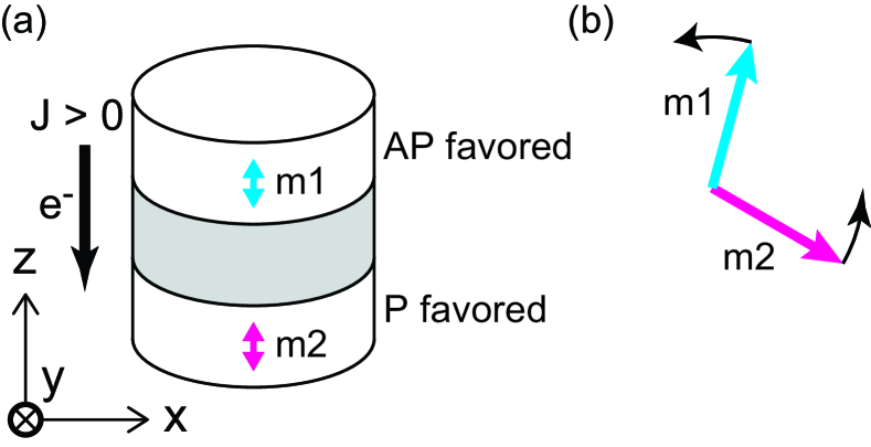
The structure of the proposed windmill neuron, illustrated in Fig. 1(a), is a spin valve, consisting of a nonmagnetic spacer layer sandwiched between two ferromagnetic layers. The spacer layer can be either a metallic layer in giant magnetoresistance devices Baibich et al. (1988); Binasch et al. (1989), or a thin insulating tunnel barrier layer in magnetic tunnel junctions Miyazaki and Tezuka (1995); Moodera et al. (1995); Yuasa et al. (2004); Parkin et al. (2004); Djayaprawira et al. (2005). The two magnetizations, m1 and m2, have preferential directions due to magnetic anisotropy. However, contrary to typical spin-valve stacks, both layers are free to switch: none of them is pinned. In the absence of spin torque, the magnetization directions are either parallel (P) or antiparallel (AP). They can point in-plane (IP) Myers et al. (1999) or out-of-plane (OOP) Mangin et al. (2006), depending on the dominant source of anisotropy. When a dc current is injected in the spin valve, perpendicularly to the layer planes, the torques on the two magnetizations tend to induce rotations in the same direction, as illustrated in Fig. 1(b). The direction of rotation is set by the sign of the applied dc current.

III MODEL

It has been predicted, as well as experimentally observed that this torque configuration can generate a windmill-like motion of the two magnetizations Gupta et al. (2016); Choi et al. (2016); Thomas et al. (2017). The equations of motion of the magnetizations are given by the Landau-Lifschitz-Gilbert-Slonczewski (LLGS) equation Slonczewski (1996); Berger (1996); Stiles and Miltat (2006)$\colon$

$$\frac{\partial\textbf{{m}}_{1}}{\partial t}=-\gamma\textbf{{m}}_{1}\times \textbf{{H}}_{\rm eff1}+\alpha\textbf{{m}}_{1}\times\frac{\partial\textbf{{m}}_{1}}{\partial t}$$

$$-\gamma\tau_{\rm st1}\textbf{{m}}_{1}\times(\textbf{{m}}_{1}\times\textbf{{m}}_{2}),$$ (1)

$$\frac{\partial\textbf{{m}}_{2}}{\partial t}=-\gamma\textbf{{m}}_{2}\times \textbf{{H}}_{\rm eff2}+\alpha\textbf{{m}}_{2}\times\frac{\partial\textbf{{m}}_{2}}{\partial t}$$

$$+\gamma\tau_{\rm st2}\textbf{{m}}_{2}\times(\textbf{{m}}_{2}\times\textbf{{m}}_{1}).$$ (2)

Here, $t$ and $\gamma$ are the time and the electron gyromagnetic ratio. The second term on the right-hand side of Eqs. (III) and (III) is the damping-torque term where $\alpha$ is the Gilbert damping constant. In this article, $\alpha=0.01$ is assumed. Hereafter, $i$ in the subscript represents the quantities of m_i layer with $i=1$ or 2. $\tau_{st1}$, and $\tau_{st2}$ represent the coefficient of the Slonczewski torque$\colon$

$$\tau_{sti}=\frac{\hbar}{2}\frac{1}{\mu_{0}M_{\rm s}}\frac{1}{d_{i}}\frac{J}{|e|}P.$$ (3)

Here, $\hbar$ is the Dirac constant, $\mu_{0}$ is the vacuum permeability, $M_{s}$ is the saturation magnetization, $d_{i}$ is the thickness of layer i, $e$ is the electron charge, $J$ is the current density and $P$ is the spin polarization. In the rest of the article, we take $P=0.6$.

$\textbf{{H}}_{{\rm eff}i}$ is the effective field expressed as

$$\textbf{{H}}_{\rm eff}=\textbf{{H}}_{\rm anis}+\textbf{{H}}_{\rm dip}.$$ (4)

Hereafter the layer index, $i$, is abbreviated. $\textbf{{H}}_{\rm anis}$ represents the anisotropy field expressed as$\colon$

$$\textbf{{H}}_{\rm anis}=\frac{2K}{\mu_{0}M_{\rm s}}m_{z}.$$ (5)

Here $K$ represents the anisotropy constant. In the spin valve shown in Fig. 1(a), $K=115$ kJ/m³ is assumed in m1, and $K=70$ kJ/m³ is assumed in m2. $\textbf{{H}}_{\rm dip}$ represents the dipolar field expressed as

$$\textbf{{H}}_{\rm dip}=-M_{\rm s}\left(N_{x}m_{x},N_{y}m_{y},N_{z}m_{z}\right).$$ (6)

Here $N_{x}$, $N_{y}$ and $N_{z}$ are the demagnetization coefficients Beleggia et al. (2005).

IV RESULTS

To highlight the principle of windmill neurons, we first neglect the dipolar-field interactions between the two magnetic layers in Fig. 1(a) and consider that they behave as macrospins with uniform magnetizations.

Figure 2: (a) Times traces of magnetization switching (macrospin simulations for a spin valve with out-of-plane (OOP) magnetized layers without dipolar-field interaction between the two ferromagnetic layers, SV_OOP1) (b) Corresponding resistance time trace. In (a) and (b), $J$ is positive and the normalized current density is $J/J_{th}=1.5$.

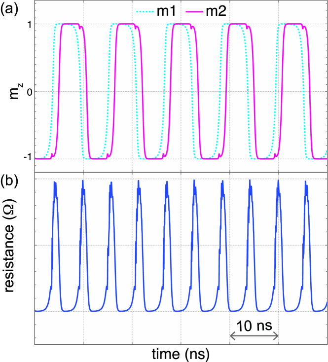
Fig. 2(a) shows macrospin simulations of magnetic switching in these conditions, for out-of-plane magnetized layers that differ only through their anisotropy constants$\colon$ $K_{\rm m1}$ = 115 kJ/m³ and $K_{\rm m2}$ = 70 kJ/m³ (The other magnetic parameters are indicated as SV_OOP1 in TABLE I). The windmill motion induces sustained switching of the magnetizations one after the other at $J\geq J_{th}=1.0$ MA/cm² where $J_{th}$ is the threshold current density for sustained windmill switching. The repeated magnetic switches give rise to changes in the device resistance ($R$) through magnetoresistance (MR) effects$\colon$ $R=(R_{AP}+R_{P})/2-[(R_{AP}-R_{P})/2]\cos\hat{\theta}_{12}$ where $R_{P}$ ($R_{AP}$) is the resistance in the parallel (antiparallel) configuration and $\hat{\theta}_{12}$ is the angle between m1 and m2. Since the injected current is dc, the resulting voltage variations across the spin valve, i.e., $V=R\times I_{dc}$, are proportional to the resistance variations. In this article we always consider a MR ratio $(R_{AP}-R_{P})/R_{P}$ of 100% and $R_{P}=100$ $\Omega$ assuming that spin valves are magnetic tunnel junctions. The resistance variations corresponding to the magnetic switches in Fig. 2(a) are plotted in Fig. 2(b). A spiking behavior similar to neuron responses is observed. The time scales of these relaxation oscillations are set by the switching times of the two layers. Here the long charging period corresponds to the switching of m1 and the short discharge period to the switching of m2.

The asymmetry of the switching times comes from the different anisotropy constants of the layers used in the simulations ($K_{\rm m1}$ = 115 kJ/m³ and $K_{\rm m2}$ = 70 kJ/m³). Indeed, the magnetization switching time $T_{SW}$ under spin torque is proportional to $1/(J-J_{th}^{(0)})$ Sun (2000) where $J_{th}^{(0)}$ is the individual threshold current density for switching Choi et al. (2016). Layers with higher anisotropy $K$ are more difficult to be switched, and have a larger threshold current density $J_{th}^{(0)}$. In our case, we find through simulations that $J_{th1}^{(0)}$ and $J_{th2}^{(0)}$ are respectively equal to 0.95 MA/cm² and 0.49 MA/cm² where m2 (m1) is fixed at the equilibrium state during the evaluation of $J_{th1}^{(0)}$ ($J_{th2}^{(0)}$). The switching times during the windmill motion for the two magnetic layers as a function of current density are plotted in Fig. 3(a) (solid curves), together with the corresponding fits in $T_{SWi}=c_{i}/(J-J_{thi}^{\prime})$ (dotted curve and dotted-dashed curve).

Figure 3: (a) Average switching times ($T_{SW1}$ and $T_{SW2}$) for m1 (solid triangles on solid curve) and m2 (solid circles on solid curves) as a function of current density. Fits by $ci/(J-J_{thi}^{\prime})$ (dotted curve and dotted-dashed curve). (b) Resistance times traces at $J=+1.75$ MA/cm² (thick solid curve), +1.25 MA/cm² (thin solid curve), -1.25 MA/cm² (thin dotted curve), -1.75 MA/cm² (thick dotted curve). (c) Frequency as a function of current density for negative and positive current densities.

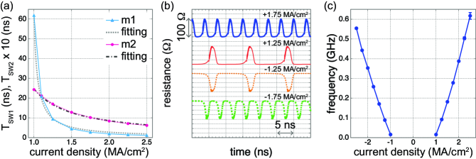
Here, $c_{i}$ and $J_{thi}^{\prime}$ are fitting parameters. The agreement between the analytical prediction of Ref. Sun (2000) and our simulations is excellent. The fitting yields $J_{th1}^{\prime}=0.954\pm 0.002$ MA/cm², $c_{1}=4.088\pm 0.215$ ns$\cdot$MA/cm², $J_{th2}^{\prime}=0.471\pm 0.015$ MA/cm², and $c_{2}=1.305\pm 0.031$ ns$\cdot$MA/cm². The threshold currents extracted from the switching times $J_{th1}^{\prime}$ ($J_{th2}^{\prime}$) agree well with the previously determined threshold currents $J_{th1}^{(0)}$ ($J_{th2}^{(0)}$). These results show that the response of the windmill neuron can be tuned by dc current. Traces at different dc current densities are shown in Fig. 3(b), and the evolution of the frequency as a function of current is plotted in Fig. 3(c). As determined experimentally and numerically in previous studies Gupta et al. (2016); Choi et al. (2016); Thomas et al. (2017), the frequency increases with an increase of $|J|$. Note that the shape of spikes can also be tuned by controlling the switching time ratio through materials engineering of the two layers ($M_{s}$, $P$ etc.).

V Occurrence of chaos

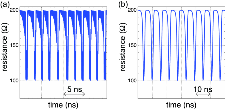
Fig. 4 compares resistance versus time traces simulated through macrospin equations of motion for in-plane (Fig. 4(a)) and out-of-plane magnetized spin valves (Fig. 4(b)) (the structure of the in-plane magnetized spin valve, SV_IP1, and its parameters are shown in Fig. 6(c) and TABLEs I and II). As can be seen, the trace in the out-of-plane case is highly regular whereas apparent fluctuation affects the periodicity of switching in the in-plane case, even if temperature induced fluctuations are not included in the simulations.

This chaotic switching of in-plane spin valves Montoya et al. under windmill motion can be interpreted in the following way. For windmill motion, the switching of one layer toggles the switching of the other. Indeed, magnetization m1 wants to achieve the AP configuration whereas m2 wants to maintain a P configuration (and inversely for a reversed sign of the current density), therefore the P and AP configurations become consecutively unstable. But the switching trajectories are very different for in-plane and out-of-plane magnetized samples. As shown in Fig. 5(a), for in-plane magnetized samples, the strong anisotropy distorts the trajectories in a clamshell shape. Let us consider the situation where one of the magnetizations, m2, is close to equilibrium and the other one m1, is switching towards m2. The switching of m1 from one hemisphere to the other is strongly determined by the exact magnetization dynamics in the narrow window highlighted in Fig. 5(a). In this window, the angle between magnetizations $\hat{\theta}_{12}$ that gives the torque strength is also strongly varying. Therefore, small variations in the position of m2 will strongly influence the switching of m1. This high coupling between degrees of freedom induces a high sensitivity of magnetization reversal to initial conditions and can favor the appearance of chaos. The situation is different for out-of-plane magnetized samples, where precessions remain mostly circular during the whole switching of m1 (Fig. 5(b)) and are therefore much less sensitive to fluctuations of m2.

Figure 4: Resistance time traces for (a) in-plane and (b) out-of-plane magnetized layers at negative $J$ with $J/J_{th}=1.5$.

Figure 5: Sketch of magnetization orbits of m1 for (a) in-plane and (b) out-of-plane magnetized layers at negative $J_{th}$.

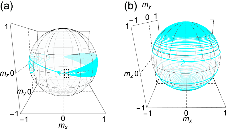
Until now we have not included the dipolar-field interaction between the magnetic layers in the simulations. The dipolar-field interaction is expected to enhance strongly the chaoticity of the system because it increases coupled degrees of freedom. Indeed, if the dipolar-field interaction exists, the switching of m2 will strongly depend on the direction of m1 (and reciprocally), yielding an increased sensitivity of the repeated magnetization switching events on initial conditions.

VI Tuning chaos by structure

The strength of the dipolar-field interaction between layers (dipolar coupling) can be controlled by tuning the anisotropy and by tuning the stack. In this section we compare the windmill dynamics in the different structures sketched in Fig. 6.

Figure 6: Sketch of the different structures$\colon$ (a) macrospin out-of-plane (OOP) spin valve without dipolar coupling (SV_OOP1), (b) micromagnetic OOP spin valve with dipolar coupling (SV_OOP2), (c) macrospin in-plane (IP) spin valve without dipolar coupling (SV_IP1), (d) micromagnetic IP spin valve with antiferromagnetically-coupled layers (m_A1 and m_A2) and with dipolar coupling (SV_IP2), (e) micromagnetic IP spin valve with dipolar coupling (SV_IP3). The axis $x$ ($z$) is parallel to the major axis of the ellipse (out-of-plane direction). Typical traces of the resistance versus time and the corresponding recurrence plots are shown below each case for $J/J_{th}=1.5$.

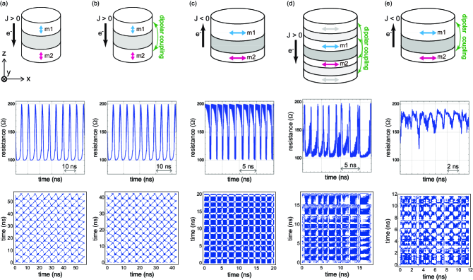
Fig. 6(a) shows an out-of-plane bilayer macrospin spin valve simulated without dipolar-field interaction (SV_OOP1). The dipolar-field interaction is included in the micromagnetic simulations of the out-of-plane bilayer (SV_OOP2) of Fig. 6(b) (micromagnetic simulations are described in the Appendix A). However, the dipolar-field interaction in the out-of-plane configuration is expected to be small because of the small $M_{s}$. Fig. 6(c) shows an in-plane bilayer macropin spin valve without the dipolar-field interaction (SV_IP1). Fig. 6(d) shows a structure with a more complicated stack, where the free layers are each composed of two antiferromagnetically coupled layers (SV_IP2). The dipolar field between the two free layers is expected to be strongly minimized in this configuration thanks to flux closure. Finally Fig. 6(e) shows an in-plane bilayer spin valve (SV_IP3) including the dipolar-field interaction which is expected to be strong in this configuration. Because of the dipolar-field interaction, SV_IP3 favors AP magnetization configuration. As a result, the switching from AP to P configuration is often interrupted, and the resistance oscillates in a higher range around 150 - 200 $\Omega$.

Table 1: Structures under study (SV_OOP1, SV_OOP2, SV_IP1, SV_IP2, and SV_IP3), simulation method, and threshold current density ($J_{th}$). OOP1, OOP2, IP1, IP2 are the labels of magnetic layers whose parameters are summarized in TABLE II. In all structures, the spacer layer between m1 and m2 has the thickness of 1 nm and its $J_{\rm RKKY}=0$. In (d) SV_IP2, the spacer layer between m1 and m_A1 (m2 and m_A2) has the thickness of 0.7 nm and its $J_{\rm RKKY}=-0.1$ mJ/m².

Structure	(a) SVOOP1	(b) SVOOP2	(c) SVIP1	(d) SVIP2	(e) SVIP3
mA1	—	—	—	IP1	—
m1	OOP1	OOP1	IP1	IP1	IP1
m2	OOP2	OOP2	IP2	IP2	IP2
mA2	—	—	—	IP2	—
Simulation method	Macrospin	Micromagnetics	Macrospin${}^{\text{a}}$	Micromagnetics${}^{\text{b}}$	Micromagnetics${}^{\text{b}}$
$J_{th}(>0)$ (MA/cm2) $J_{th}(<0)$ (MA/cm2)	1.0 -1.0	1.1 -1.1	— -6.0	21 -23	—${}^{\text{c}}$ -34

Table 2: Parameters of magnetic layers: OOP1, OOP2, IP1, and IP2. $S$ is the area of the base.

Magnetic layer	OOP1	OOP2	IP1	IP2
$S$ (nm2)	$16\times 16\times\pi$	$16\times 16\times\pi$	$30\times 10\times\pi$	$30\times 10\times\pi$
$d$ (nm)	1	1	1	0.5
$M_{s}$ (kA/m)	200	200	1300	1300
$K$ (kA/m3)	115	70	0	0

Typical time traces are shown below each structure. As can be seen, the degree of chaos seems to increase when the anisotropy changes from out-of-plane (Fig. 6 (a)-(b)) to in-plane (Fig. 6(c)). It also increases in the in-plane configuration when the strength of dipolar-interaction between layers increases (Fig. 6 (c)-(d)-(e)).

In order to evaluate more thoroughly the degree of chaos in structures shown in Fig. 6, we have used three methods: quality factor (Q factor), Recurrence Quantification Analysis (RQA) Eckmann et al. (1987); Marwan et al. (2007); Webber and Zbilut (1994); Marwan and Kurths (2002), and Lyapunov exponent Wolf et al. (1985). Low Q factor and low $DET$, $L$, $L_{\rm max}$ and $ENTR$ in RQA indicate high degree of chaos, and high Lyapunov exponent indicates high degree of chaos. The evaluated values at $J/J_{th}=1.5$ are summarized in TABLE III.

Table 3: Evaluated degree of chaos: quality factor (Q factor), [$DET$, $L$, $L_{\rm max}$, $ENTR$] of Recurrence Quantification Analysis (RQA), and Lyapunov exponent of SV_OOP1, SV_OOP2, SV_IP1, SV_IP2, and SV_IP3 at $J/J_{th}=1.5$.

Method	(a) SVOOP1	(b) SVOOP2	(c) SVIP1	(d) SVIP2	(e) SVIP3
Q factor	$>10^{4}$	440	11	2.5	3.7
$DET(\%)$	0.88	0.66	0.10	0.066	0.11
$L$	5.4	4.5	2.4	2.2	2.3
$L_{\rm max}$	3100	650	40	8	9
$ENTR$	1.9	1.7	0.81	0.44	0.69
Lyapunov exponent (Gbit/s)	0.14	0.89	4.5	5.0	6.9

First, we have extracted a quality factor (Q factor) of for the interspike time interval from each time trace. In Figs. 6(a), (b) and (d) (In Figs. 6(c) and (e)), each time interval where $R\leq 150$ $\Omega$ ($R\geq 150$ $\Omega$) is defined as the interspike time interval. The Q factor is evaluated as $T_{I}/\sigma_{I}$ during 10 sets of switching of m1 and m2 where $T_{I}$ ($\sigma_{I}$) is the average value (standard deviation) of interspike time interval. As we see the enhanced chaotic magnetization dynamics in the in-plane magnetized spin valve in Sec. V, the Q factor decreases when the anisotropy changes from out-of-plane ((a) SV_OOP1 and (b) SV_OOP2) to in-plane ((c) SV_IP1, (d) SV_IP2 and (e) SV_IP3). In (a) SV_OOP1, the Q factor exceeds our analyzable upper limit of $10^{4}$ because $\sigma_{I}=0$ in our simulation with a time step of 1 ps. The Q factor also decreases by the introduction of dipolar-field interaction between layers ([(a) SV_OOP1 v.s. (b) SV_OOP2] and [(c) SV_IP1 v.s. (d) SV_IP2 and (e) SV_IP3]). However, the flux-closure structure in Fig. 6(d) hardly improves the Q factor. Nevertheless, it recovers the full amplitude of resistance oscillation compared to Fig. 6(e) and reduces the threshold current $J_{th}$.

Then we have conducted Recurrence Quantification Analysis of $R(t)$ for each structure. Recurrence plots for each structure are shown at the bottom of Fig. 6. A recurrence plot Eckmann et al. (1987); Marwan et al. (2007) is a square matrix, in which the matrix elements correspond to those times at which a similar resistance state recurs, i.e., a plot of ${\mathfrak{R}_{\iota,\kappa}}=\Theta(\epsilon_{\iota}-\|R(t_{\iota})-R(t_{\kappa})\|)$. Here, $t_{\iota}$ and $t_{\kappa}$ are time during about 10 periods of resistance oscillation shown in the middle panels of Fig. 6. $\epsilon_{\iota}$ is a threshold distance, and $\epsilon_{\iota}=0.05$ $\Omega$ is chosen in Fig. 6. $\Theta$ is the Heaviside function, and the elements where ${\mathfrak{R}_{\iota,\kappa}}=1$ are dots in the recurrence plots. In other words, the elements where $R(t_{\iota})\sim R(t_{\kappa})$ appear as dots in the plots. Trivial dots at the matrix diagonal elements at $t_{\iota}=t_{\kappa}$ are removed. A perfectly periodic oscillator will have dots mainly along the diagonal. In Figs. 6(d) and (e), the plots show patterns with reduced regularity reflecting their high degree of chaos compared to the cases of Figs. 6(a)-(c).

Results of Recurrence Quantification Analysis Webber and Zbilut (1994); Marwan and Kurths (2002); Marwan et al. (2007), i.e., $DET$, $L$, $L_{\rm max}$ and $ENTR$ are summarized in the middle of TABLE III. $DET$, $L$, $L_{\rm max}$, and $ENTR$ are quantities characterized by the diagonal lines in a recurrence plot. The lengths of diagonal lines are directly related to the ratio of predictability inherent to the system. Suppose that the states at times ι and κ are neighboring. If the system exhibits predictable behavior, similar situations will lead to a similar future, i.e., the probability for $R(t_{\iota})\sim R(t_{\kappa})$ is high. For perfectly periodic systems, this leads to infinitely long diagonal lines. In contrast, if the system is chaotic, the probability for $R(t_{\iota})\sim R(t_{\kappa})$ will be small and we only find single points or short lines. In accordance with the evaluated Q factors, $DET$, $L$, $L_{\rm max}$, and $ENTR$ decreases when the anisotropy changes from out-of-plane to in-plane. They also decrease by the introduction of dipolar-interaction between layers.

Then we have determined the Lyapunov exponent from each time trace Wolf et al. (1985). The Lyapunov exponent is a quantity that characterizes the rate of separation of infinitesimally close trajectories in dynamic systems. Lyapunov exponents were evaluated with about 100 periods of resistance oscillation for each structure. As we have expected, the Lyapunov exponent, characterizing the degree of chaos, increases when the anisotropy changes from out-of-plane to in-plane. It also increases in the in-plane configuration when the strength of dipolar interaction between layers increases. These results show that the degree of chaos can be tuned in a wide range by engineering the magnetic stack and anisotropies, which is suitable for various neuromorphic computing applications.

VII Tuning chaos by current

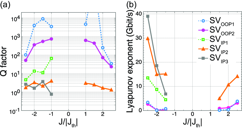
We also checked the tunability of chaos by current. The evaluated current density dependence of quality factors (Q factors) and Lyapunov exponents are shown in Fig. 7. $J/|J_{th}|$ represents the current density normalized by the threshold current density for each polarity of current. The Lyapunov exponents at $J/|J_{th}|=\pm 1$ are not shown because the too long interspike time interval against pulse width makes evaluation of Lyapunov exponent itself impossible and long simulations of 100 periods are not possible with our computational capacity. Both trends in Figs. 7(a) and (b) show that the degree of chaos is increased by increasing the magnitude of $J/|J_{th}|$. A cause of the increased degree of chaos at large $|J/J_{th}|$ can be the increased instability of m2 during the interspike time interval. Fluctuations of m2 strongly vary the angle between magnetizations $\hat{\theta}_{12}$ that gives the torque strength. Therefore, the switching of m1 will be complex through the dynamics of m2. The trend in Fig. 7 means that the degree of chaos can be tuned in a wide range by the dc current. The tunability of chaos by current is quite beneficial because it enables the control of chaos in real-time in a ready-made circuit.

Figure 7: (a) $J/|J_{th}|$ dependence of Q factor of interspike time interval and (b) Lyapunov exponent. Open circles on dotted lines are for SV_OOP1. Solid circles on solid lines are for SV_OOP2. Open squares on dotted lines are for SV_IP1. Solid triangles on solid lines are for SV_IP2. Solid squares on solid lines are for SV_IP3.

VIII conclusion

We proposed a simple way to imitate neuron spiking in high-magnetoresistance nanoscale spin valves where both magnetic layers are free and can be switched by spin torque. Our numerical-simulation results show that the windmill motion induced by spin torque in the proposed spintronic neurons gives rise to spikes whose shape and frequency can be tuned through the amplitude of injected dc current. We also found that these devices can exhibit chaotic oscillations. By evaluating the quality factors of interspike time intervals and Lyapunov exponents, as well as conducting Recurrence Quantification Analysis for the time evolutions of resistance, we demonstrate that the degree of chaos can be tuned in a wide range by engineering the magnetic stack and anisotropies and by changing the dc current. The degree of chaos increases when the anisotropy of the free layer changes from out-of-plane to in-plane. It also increases when the dipolar-field interaction between the free layers increases. The proposed spintronic neuron is a promising building block for hardware neuromorphic chips leveraging complex non-linear dynamics for computing.

Appendix A MODEL IN MICROMAGNETIC SIMULATIONS

In micromagnetic simulations, ${\bm{m}}_{i}=(m_{xi}$, $m_{yi}$, $m_{zi})$ of Eqs. (III) and (III) mean the unit magnetization vector of a unit cell at the position ${\bm{r}}_{i}$, ${\bm{m}}_{i}({\bm{r}}_{i})$. The simulations were conducted with the simulation code, SpinPM Spi . In micromagnetic simulations of this article, each magnetic layer is divided into unit cells with the area of 4 nm$\times$4 nm. In the third term on the right side of Eqs. (III) and (III), i.e., the Slonczewski-torque term, $x$ and $y$ components of ${\bm{r}}_{1}$ and ${\bm{r}}_{2}$ are the same.

In Eqs. (III) and (III), $\textbf{{H}}_{\rm eff}$ is the effective field expressed as

$$\textbf{{H}}_{\rm eff}=\textbf{{H}}_{\rm exch}+\textbf{{H}}_{\rm anis}+\textbf{{H}}_{\rm dip}+\textbf{{H}}_{\rm RKKY}.$$ (7)

$\textbf{{H}}_{\rm exch}$ represents the exchange field expressed as

$$\textbf{{H}}_{\rm exch}=\frac{2A}{\mu_{0}M_{\rm s}}\nabla^{2}\textbf{{m}}.$$ (8)

$A$ is the exchange constant. In the micromagnetic simulations, it is assumed to be $A=2\times 10^{-11}$ J/m in this article. $\textbf{{H}}_{\rm dip}$ represents the dipolar field. $\textbf{{H}}_{\rm dip}$ on the position ${\bm{r}}$ is expressed as

$$\textbf{{H}}_{\rm dip} =-\frac{M_{\rm s}}{4\pi}\int_{Vol}\left[\frac{\textbf{{m}}(\textbf{{r}}^{\prime})}{|\textbf{{r}}-\textbf{{r}}^{\prime}|^{3}}\right.$$

$$\hskip 62.59605pt-\left.\frac{3\left[\textbf{{m}}(\textbf{{r}}^{\prime})\cdot(\textbf{{r}}-\textbf{{r}}^{\prime})\right]}{|\textbf{{r}}-\textbf{{r}}^{\prime}|^{5}}(\textbf{{r}}-\textbf{{r}}^{\prime})\right]d\textbf{{r}}^{\prime}.$$ (9)

Here the integral is performed over the volume ($Vol$) including all magnetic layers. $\textbf{{H}}_{\rm RKKY}$ represents the RKKY coupling field expressed as

$$\textbf{{H}}_{\rm RKKY}=\frac{J_{\rm RKKY}}{\mu_{0}M_{\rm s}d}\nabla\left(\textbf{{m}}\cdot\textbf{{m}}_{{\rm A}}\right).$$ (10)

Here, $J_{\rm RKKY}$ is the exchange coupling constant. $\textbf{{H}}_{\rm RKKY}$ is considered only in the spin valve shown in Fig. 6(d). ${\bm{m}}_{\rm A}$ represents the unit magnetization vector of a ferromagnetic layer which is antiferromagnetically-coupled with m, and $J_{\rm RKKY}=-0.1$ mJ/m² is assumed. In the scalar product, $x$ and $y$ components of ${\bm{r}}$ in ${\bm{m}}({\bm{r}})$ and ${\bm{r}}_{\rm A}$ in ${\bm{m}}_{\rm A}({\bm{r}}_{\rm A})$ are the same.

References

- Merolla et al. (2014) Paul A. Merolla, John V. Arthur, Rodrigo Alvarez-Icaza, Andrew S. Cassidy, Jun Sawada, Filipp Akopyan, Bryan L. Jackson, Nabil Imam, Chen Guo, Yutaka Nakamura, Bernard Brezzo, Ivan Vo, Steven K. Esser, Rathinakumar Appuswamy, Brian Taba, Arnon Amir, Myron D. Flickner, William P. Risk, Rajit Manohar, and Dharmendra S. Modha, “A million spiking-neuron integrated circuit with a scalable communication network and interface,” Science 345, 668–673 (2014).
- Hoppensteadt and Izhikevich (1999) Frank C. Hoppensteadt and Eugene M. Izhikevich, “Oscillatory neurocomputers with dynamic connectivity,” Phys. Rev. Lett. 82, 2983–2986 (1999).
- Aonishi et al. (1999) Toru Aonishi, Koji Kurata, and Masato Okada, “Statistical mechanics of an oscillator associative memory with scattered natural frequencies,” Phys. Rev. Lett. 82, 2800–2803 (1999).
- Jaeger and Haas (2004) Herbert Jaeger and Harald Haas, “Harnessing nonlinearity: Predicting chaotic systems and saving energy in wireless communication,” Science 304, 78–80 (2004).
- Maass et al. (2002) Wolfgang Maass, Thomas Natschläger, and Henry Markram, “Real-time computing without stable states a new framework for neural computation based on perturbations,” Neural Computation 14, 2531–2560 (2002).
- Pickett et al. (2013) Matthew D. Pickett, Gilberto Medeiros-Ribeiro, and R. Stanley Williams, “A scalable neuristor built with mott memristors,” Nature Materials 12, 114–117 (2013).
- Segall et al. (2017) K. Segall, M. LeGro, S. Kaplan, O. Svitelskiy, S. Khadka, P. Crotty, and D. Schult, “Synchronization dynamics on the picosecond time scale in coupled josephson junction neurons,” Phys. Rev. E 95, 032220 (2017).
- Feng et al. (2008) X. L. Feng, C. J. White, A. Hajimiri, and M. L. Roukes, “A self-sustaining ultrahigh-frequency nanoelectromechanical oscillator,” Nature Nanotechnology 3, 342–346 (2008).
- Slonczewski (1996) J. C. Slonczewski, “Current-driven excitation of magnetic multilayers,” J. Magn. Magn. Mater. 159, L1–L7 (1996).
- Berger (1996) L. Berger, “Emission of spin waves by a magnetic multilayer traversed by a current,” Phys. Rev. B 54, 9353–9358 (1996).
- Kiselev et al. (2003) S. I. Kiselev, J. C. Sankey, I. N. Krivorotov, N. C. Emley, R. J. Schoelkopf, R. A. Buhrman, and D. C. Ralph, “Microwave oscillations of a nanomagnet driven by a spin-polarized current,” Nature 425, 380–383 (2003).
- Torrejon et al. (2017) Jacob Torrejon, Mathieu Riou, Flavio Abreu Araujo, Sumito Tsunegi, Guru Khalsa, Damien Querlioz, Paolo Bortolotti, Vincent Cros, Kay Yakushiji, Akio Fukushima, Hitoshi Kubota, Shinji Yuasa, Mark D. Stiles, and Julie Grollier, “Neuromorphic computing with nanoscale spintronic oscillators,” Nature 547, 428–431 (2017).
- Pikovsky (2003) Arkady Pikovsky, Synchronization A universal concept nonlinear sciences (Cambridge University Press, 2003).
- Buzsaki (2011) Gyorgy Buzsaki, Rhythms of the Brain (Oxford University Press, 2011).
- Gupta et al. (2016) Gaurav Gupta, Zhifeng Zhu, and Gengchiau Liang, “Switching based spin transfer torque oscillator with zero-bias field and large tuning-ratio,” arXiv:1611.05169 [cond-mat] (2016).
- Choi et al. (2016) R. Choi, J. A. Katine, S. Mangin, and E. E. Fullerton, “Current-induced pinwheel oscillations in perpendicular magnetic anisotropy spin valve nanopillars,” IEEE Transactions on Magnetics 52, 1–5 (2016).
- Thomas et al. (2017) L. Thomas, M. Benzaouia, S. Serrano-Guisan, G. Jan, S. Le, Y. Lee, H. Liu, J. Zhu, J. Iwata-Harms, R. Tong, Y. Yang, V. Sundar, S. Patel, J. Haq, D. Shen, R. He, V. Lam, J. Teng, P. Liu, A. Wang, T. Zhong, T. Torng, and P. Wang, “Spin transfer torque driven dynamics of the synthetic antiferromagnetic reference layer of perpendicular MRAM devices,” in 2017 IEEE International Magnetics Conference (INTERMAG) (2017) pp. 1–1.
- (18) SpinPM is a micromagnetic code developed by the Istituto P.M. srl (Torino, Italy - www.istituto-pm.it) based on a forth order Runge-Kutta numerical scheme with an adap-tative time-step control for the time integration.
- Slonczewski and Sun (2007) J. C. Slonczewski and J. Z. Sun, “Theory of voltage-driven current and torque in magnetic tunnel junctions,” Journal of Magnetism and Magnetic Materials Proceedings of the 17th International Conference on Magnetism, 310, 169–175 (2007).
- Softky and Koch (1993) W. R. Softky and C. Koch, “The highly irregular firing of cortical cells is inconsistent with temporal integration of random EPSPs,” J. Neurosci. 13, 334–350 (1993).
- Kumar et al. (2017) Suhas Kumar, John Paul Strachan, and R. Stanley Williams, “Chaotic dynamics in nanoscale NbO mott memristors for analogue computing,” Nature 548, 318–321 (2017).
- Appeltant et al. (2011) L. Appeltant, M. C. Soriano, G. Van der Sande, J. Danckaert, S. Massar, J. Dambre, B. Schrauwen, C. R. Mirasso, and I. Fischer, “Information processing using a single dynamical node as complex system,” Nature Communications 2, 468 (2011).
- Baibich et al. (1988) M. N. Baibich, J. M. Broto, A. Fert, F. Nguyen Van Dau, F. Petroff, P. Etienne, G. Creuzet, A. Friederich, and J. Chazelas, “Giant magnetoresistance of (001)Fe/(001)Cr magnetic superlattices,” Phys. Rev. Lett. 61, 2472–2475 (1988).
- Binasch et al. (1989) G. Binasch, P. Grünberg, F. Saurenbach, and W. Zinn, “Enhanced magnetoresistance in layered magnetic structures with antiferromagnetic interlayer exchange,” Phys. Rev. B 39, 4828–4830 (1989).
- Miyazaki and Tezuka (1995) T. Miyazaki and N. Tezuka, “Giant magnetic tunneling effect in Fe/Al2O3/Fe junction,” 139, L231–L234 (1995).
- Moodera et al. (1995) J. S. Moodera, Lisa R. Kinder, Terrilyn M. Wong, and R. Meservey, “Large magnetoresistance at room temperature in ferromagnetic thin film tunnel junctions,” Phys. Rev. Lett. 74, 3273–3276 (1995).
- Yuasa et al. (2004) Shinji Yuasa, Taro Nagahama, Akio Fukushima, Yoshishige Suzuki, and Koji Ando, “Giant room-temperature magnetoresistance in single-crystal Fe/MgO/Fe magnetic tunnel junctions,” Nat. Mater. 3, 868–871 (2004).
- Parkin et al. (2004) Stuart S. P. Parkin, Christian Kaiser, Alex Panchula, Philip M. Rice, Brian Hughes, Mahesh Samant, and See-Hun Yang, “Giant tunnelling magnetoresistance at room temperature with MgO (100) tunnel barriers,” Nat. Mater. 3, 862–867 (2004).
- Djayaprawira et al. (2005) David D. Djayaprawira, Koji Tsunekawa, Motonobu Nagai, Hiroki Maehara, Shinji Yamagata, Naoki Watanabe, Shinji Yuasa, Yoshishige Suzuki, and Koji Ando, “230% room-temperature magnetoresistance in CoFeB/MgO/CoFeB magnetic tunnel junctions,” Appl. Phys. Lett. 86, 092502 (2005).
- Myers et al. (1999) E. B. Myers, D. C. Ralph, J. A. Katine, R. N. Louie, and R. A. Buhrman, “Current-induced switching of domains in magnetic multilayer devices,” Science 285, 867–870 (1999).
- Mangin et al. (2006) S. Mangin, D. Ravelosona, J. A. Katine, M. J. Carey, B. D. Terris, and Eric E. Fullerton, “Current-induced magnetization reversal in nanopillars with perpendicular anisotropy,” Nat. Mater 5, 210–215 (2006).
- Stiles and Miltat (2006) Mark D. Stiles and Jacques Miltat, “Spin-transfer torque and dynamics,” in Spin Dynamics in Confined Magnetic Structures III, Topics in Applied Physics, Vol. 101, edited by Burkard Hillebrands and André Thiaville (Springer Berlin Heidelberg, 2006) pp. 225–308.
- Beleggia et al. (2005) M. Beleggia, M. De Graef, Y. T. Millev, D. A. Goode, and G. Rowlands, “Demagnetization factors for elliptic cylinders,” J. Phys. D: Appl. Phys. 38, 3333 (2005).
- Sun (2000) J. Z. Sun, “Spin-current interaction with a monodomain magnetic body: A model study,” Phys. Rev. B 62, 570–578 (2000).
- (35) Eric Arturo Montoya, Salvatore Perna, Yu-Jin Chen, Jordan A. Katine, Massimiliano d’Aquino, Claudio Serpico, and Ilya N. Krivorotov, “Magnetization reversal driven by low dimensional chaos in a nanoscale ferromagnet,” arXiv:1806.03383 [cond-mat] 1806.03383 .
- Eckmann et al. (1987) J.-P. Eckmann, S. Oliffson Kamphorst, and D. Ruelle, “Recurrence plots of dynamical systems,” Europhys. Lett. 4, 973 (1987).
- Marwan et al. (2007) Norbert Marwan, M. Carmen Romano, Marco Thiel, and Jürgen Kurths, “Recurrence plots for the analysis of complex systems,” Physics Reports 438, 237–329 (2007).
- Webber and Zbilut (1994) C. L. Webber and J. P. Zbilut, “Dynamical assessment of physiological systems and states using recurrence plot strategies,” Journal of Applied Physiology 76, 965–973 (1994).
- Marwan and Kurths (2002) Norbert Marwan and Jürgen Kurths, Nonlinear analysis of bivariate data with cross recurrence plots (2002).
- Wolf et al. (1985) Alan Wolf, Jack B. Swift, Harry L. Swinney, and John A. Vastano, “Determining lyapunov exponents from a time series,” 16, 285–317 (1985).