Towards Fast and Energy-Efficient Binarized Neural Network Inference on FPGA

Abstract.

Binarized Neural Network (BNN) removes bitwidth redundancy in classical CNN by using a single bit (-1/+1) for network parameters and intermediate representations, which has greatly reduced the off-chip data transfer and storage overhead. However, a large amount of computation redundancy still exists in BNN inference. By analyzing local properties of images and the learned BNN kernel weights, we observe an average of $\sim$78% input similarity and $\sim$59% weight similarity among weight kernels, measured by our proposed metric in common network architectures. Thus there does exist redundancy that can be exploited to further reduce the amount of on-chip computations.

Motivated by the observation, in this paper, we proposed two types of fast and energy-efficient architectures for BNN inference. We also provide analysis and insights to pick the better strategy of these two for different datasets and network models. By reusing the results from previous computation, much cycles for data buffer access and computations can be skipped. By experiments, we demonstrate that 80% of the computation and 40% of the buffer access can be skipped by exploiting BNN similarity. Thus, our design can achieve 17% reduction in total power consumption, 54% reduction in on-chip power consumption and 2.4$\times$ maximum speedup, compared to the baseline without applying our reuse technique. Our design also shows 1.9$\times$ more area-efficiency compared to state-of-the-art BNN inference design. We believe our deployment of BNN on FPGA leads to a promising future of running deep learning models on mobile devices.

1. Introduction

The thriving of Deep Neural Networks (DNN), especially Convolutional Neural Network (CNN), is empowered by the advance of hardware accelerators, such as GPU (NVIDIA Corporation, 2007), TPU (Jouppi et al., 2017), and neural network accelerators integrated into various embedded processors (Sim et al., 2016). The major challenges of accelerating classical CNNs, which are based on floating-point arithmetic, are (1) off-chip Dynamic Random-Access Memory (DRAM) access power overhead, and (2) on-chip data storage constraints. Many prior works have been proposed to accelerate CNNs by exploiting sparsity (Han et al., 2017) or leveraging data reuse (Chen et al., 2016).

Among all kinds of solutions to the above challenges, quantization with reduced bitwidth in network parameters and input data is one of the most promising approaches. Algorithms such as (Zhu et al., 2016; Zhou et al., 2017; Courbariaux and Bengio, 2016) have successfully reduced the bitwidth of network weights while maintaining a high precision for image classification tasks. In particular, Binary Neural Network (BNN), a binary quantized version of CNN, has been studied extensively since it can significantly alleviate the DRAM memory access overhead and on-chip storage constraints. In BNN, the multiplication and addition in traditional floating point CNN inference are replaced by more power-efficient, compact, and faster bit operations, which are suitable for reconfigurable logic like Field-Programmable Gate Array (FPGA). However, though the bitwidth in both computation and storage has been considerably reduced, the total number of Multiplication and ACcumulation (MAC) operations still remains the same. For example, binarized VGG-16 neural network  (Simonyan and Zisserman, 2014) has reduced the network storage by around 5$\times$ but it still requires many computations ( $\sim$15.5 Giga MAC operations) to do inference on one input image  (Liang et al., 2018b)(Umuroglu et al., 2017)(Kim et al., 2017).

To reduce the number of MAC operations, we leverage the key property of BNN: As the input and kernel weights of BNN are -1/+1, they both exhibit high similarity. Intuitively, the input similarity comes from the spatial continuity of the image to classify, and the kernel similarity comes from the correlation of features represented by different binarized weight kernels (Courbariaux et al., 2016). To prove this property of BNN, we studied the similarity of input and kernel across different applications and networks, as shown in Table 1. The kernel similarity is computed based on the re-ordering algorithm described in section  3.3. The average input and kernel similarity ratio is ranging from 78% $\sim$ 84% and 59% $\sim$ 64% for network models (Courbariaux and Bengio, 2016) (Lin et al., 2013). However, if the weights of BNN are binarized but the activations are finely quantized (Table 1), which is a favorable setting in many current works (Courbariaux et al., 2015), the kernel similarity is much higher than the input similarity. In other words, we see that the degree of these similarities highly depends on the dataset and network architectures.

Based on these observations, we propose an architecture of BNN accelerator that leverages input and kernel similarities to reduce the number of MAC operations at inference time. Instead of directly computing the XNOR between the input activation and kernel weights, we first check the input or kernel weight difference between the current and previous computation stage, which focuses on different image regions or different weight kernels, and then reuse the results from the previous computation. Thus, the data buffer access or MAC operations can be bypassed if there is no difference from the previous stage. Our analysis shows that 80% of the computation and 40% of the buffer access on average can be skipped in this way. As a result, our design can reduce the total power consumption by around 17% and on-chip power consumption by 54 % in comparison to the one without using our reuse method. Our design is also 1.9$\times$ more area-efficient compared to the state-of-the-art BNN accelerator.

In addition, we observed that similarites can vary for different applications. Therefore, we provide analysis and insights to pick the better one from our proposed two reuse strategies for different datasets and network models.

Table 1. Input and kernel similarity ratio across different networks and datasets. A=(8,4) means 8-bit fixed point activation input including 4-bit fractional part. LeNet-5 and NIN are trained on XNOR-Net (Rastegari et al., 2016).

Dataset	Network	Min Input Sim (%)	Avg Input Sim (%)	Max Input Sim(%)	Kernel Sim (%)
MNIST	LeNet-5	66.6	79.3	88.6	59.8
MNIST	LeNet-5, A=(8,4)	10.6	37.5	67.0	59.8
Cifar-10	BinaryNet	59.6	78.6	95.6	58.8
Cifar-10	BinaryNet, A=(8,4)	1.8	17.3	72.2	58.8
Cifar-10	NIN	51.3	83.9	97.2	64.5
Cifar-10	NIN, A=(8,4)	2.7	23.5	66.7	64.5

To sum up, we make the following contributions:

• We analyze the input and kernel similarity in BNN across different applications. We also show that the degree of similarity depends on datasets and network architectures and we generate insights to select the best strategy.

• To the best of our knowledge, we are the first to exploit input and kernel similarity to reduce computation redundancy to accelerate BNN inference. We propose two types of novel, scalable, and energy-efficient BNN accelerator design to leverage different types of similarity. Our comparison between these two accelerators provide guidelines to pick the best one or even combine them together.

• Our implementation indicates that by exploiting similarities in BNN, we can push the efficiency and speed of its inference to a higher level.

The code of this work will be made public online. The rest of this paper is organized as follows: Section 2 gives an introduction of CNN and BNN inference; Section 3 describes our motivation to exploit input and kernel similarity and presents our method; Section 4 provides the hardware architecture of the accelerator; Section 5 reports our experiments and findings; Section 6 reviews previous work on traditional accelerator design; finally, we discuss potential future work in Section 7 and conclude the paper in Section 8.

2. Background

2.1. Convolutional Neural Networks

Convolutional Neural Networks (CNNs) are commonly used for image processing, object recognition and video classification  (Simonyan and Zisserman, 2014). A convolutional layer implements a set of kernels to detect features in the input image. A kernel is defined by a set of weights $W$ and a bias term $B$. Each convolutional layer applies multiple kernels on the input where each kernel scans through the input in a sliding way, resulting in multiple output feature maps (ofmap). Note that, unlike what happens in Fully-Connected (FC) layers, the weights of a kernel are shared across different locations on the input. Formally, suppose the input vector is $X$ and weight vector of a kernel is $W$, then the ofmap $O$ of this convolution operation is the dot product between them, added by the bias $B$, and followed by a non-linear activation function $g(\cdot)$ as shown in Equation  1:

(1) $$O=g(W\cdot X+B)$$

In CNNs, a pooling layer is usually added after a convolutional layer. FC layers are often appended after several stacked convolutional blocks. During training, the ground-truth output serves as a supervision signal to learn parameters $W$ and $B$ by minimizing a loss function. After a CNN has been trained, the network inference is applied to the test image. Previous work  (Zhang et al., 2016) shows that the computation of the CNN inference is dominated by the convolution operation, which is our main focus in this work.

Thanks to the idea of weight sharing, lots of computation are actually not necessary because convolution is naturally a sliding-based operation. The goal of this paper is to reduce the computation cost of convolutions by exploiting what we have already computed so that we can reuse them instead of computing repeatedly.

2.2. Binarized Neural Networks

Recent studies identify that there is no need to employ full-precision weights and activations since CNN is highly fault-tolerant  (Sharma et al., 2018); we can preserve the accuracy of a neural network using quantized fixed-point values, which is called quantized neural network (QNN) (Hubara et al., 2016). An extreme case of QNN is Binarized Neural Network (BNN)  (Rastegari et al., 2016), which adopts weights and activations with only two possible values (e.g., -1 and +1). The most widely used binarization strategy is called deterministic binarization, as illustrated in Equation  2. This strategy is preferred because it is suitable for hardware accelerations.

(2) $$x_{b}=\text{Sign}(x)$$

Here, $x$ can be any weight or activation input and $x_{b}$ is its binarized version. It has been shown that input activation binarization causes much more degradation to the accuracy of BNN classification compared with weight binarization (Courbariaux et al., 2016; Zhou et al., 2016; Zhu et al., 2018). Thus we consider two BNN configurations: (i) Both input and weights are binarized. (ii) Input is quantized to fixed-point values and weights are binarized. These two configurations also affect our design choice and will be described in Sec 3.2. As for implementation of this paper, we mainly focus on accelerating a BNN model developed by Courbariaux et al. in (Courbariaux and Bengio, 2016). However, our proposed scheme can be employed on any BNN, which has convolution operations during inference phase. Throughout the rest of this paper, we represent the input activation vector $X$ of the BNN as $\text{IA}(h,w,c)$, corresponding to the horizontal index, vertical index, and channel index. We further denote the weight vector $W$ by $W(r,s,c,k)$, corresponding to horizontal index, vertical index, channel index and kernel index.

3. Design Principles

In this section, we first introduce the objective of our method with a key observation on BNN’s property (Sec 3.1), which drives our proposed reuse principle (Sec 3.2). Moreover, we solve an offline optimization problem to further improve the gain (Sec 3.3).

3.1. Motivation

To realize a design that can efficiently accelerate BNN inference, typically people tend to optimize an objective called throughput which can be described by frame per second (FPS) as Equation  3:

(3) $$\text{FPS}=\frac{\#\text{Multipliers}\times\text{Utilization}}{\#\text{Ops\_per\_image}}$$

where Utilization indicates the ratio of time for multipliers doing inference over the total runtime. To increase the FPS, previous BNN works seek to increase the number of multipliers by reducing the control overhead. Other works exploit a highly parallelized computation architecture that can increase the Utilization. But another orthogonal direction for increasing the FPS is by reducing the number of $Ops\_per\_image$, which has not been fully exploited in current works. In this paper, we notice that a large amount of computation redundancy exists in BNN inference. Thus, our approach aims to reduce the number of $Ops\_per\_image$ – that is to utilize the input or kernel similarities which will be discussed in section  3.2. Our work also has the advantage of reducing on-chip power consumption. Specifically, the data buffer access and computation power can be saved as a result of the reduced number of Ops_per_image.

3.2. Similarity Inspired Reuse Strategy

Recall that our objective is to reduce the number of Ops_per_image to maximize the throughput. Unlike floating-point values in CNNs, BNN has binarized weight and input after the model is trained. Thus, BNN has only two values (-1/+1), which means we have 50% chance of having the same value if we pick random two numbers in weight or input. In what follows, we introduce two types of similarity and show our statistical results.

Input similarity: Input similarity naturally exists in various datasets when we use BNN to classify images. Most natural images have spatial continuity and adjacent pixels are similar. In consequence, the binarized ofmaps are also very likely to be spatially similar.

Kernel similarity: kernel similarity comes from the affinity of features represented by different binarized weight kernels. It has been shown in literature that weight kernels of BNN are highly similar (only 42$\%$ are unique on Cifar-10 in (Courbariaux et al., 2016)). The kernel similarity can be further optimized by using the algorithm introduced in Section 3.3 which can be computed off-line.

Based on these properties, we did an experiment on multiple BNN models to evaluate the input and kernel similarities which are defined as Equation  4 and  5.

(4) $$\text{IA}(h,w,c)=\text{IA}(h,w-1,c),0<w\leq W_{m}$$

(5) $$W(r,s,c,k)=W(r,s,c,k-1),0<k\leq K$$

The input or weight similarity ratio is defined as the input or weight values that are subjected to Equation 4 and Equation 5 over the size of total input and weight values. The results are illustrated in Table  1. The reported kernel similarity is optimized by using the algorithm as described in section  3.3.

As we can see in Table  1, the BNN has different average similarity ratio in both weight and input across different models. For BinaryNet (Courbariaux and Bengio, 2016), the average input and kernel similarity are $\sim$78% and $\sim$58% respectively, which indicates a high computational redundancy in BNN inference and so does NIN on XNOR-Net (Rastegari et al., 2016). For BNN trained by XNOR-Net on MNIST, the average similarity ratio on input and weights are $\sim$79.3% and $\sim$59.8% respectively. We also observe that many of the BNN models are implemented with fixed-point input activations to maintain high classification accuracy (Zhou et al., 2016). For BNN with fixed-point input and binarized weight, the input similarity is much lower than kernel similarity as shown in Table  1. Therefore, which one is better varies case by case. The comparison and determination can be done off-line after the network and dataset are obtained.

Depends on the insights generated by our experiment results, we develop two types of neural networks acceleration strategies which exploits either weight or input similarity to reduce redundant computations. We now introduce two computation reuse strategies to leverage these two types of similarity respectively.

Figure 1. Method of exploiting input and kernel similarity. (1) shows the computation without using the reuse strategy. (2) illustrates the computation with reuse strategy. The computation of STAGE II reuse the computation result from STAGE I by exploiting (a) input similarity (b) kernel similarity

In Figure  1, we use a simple example to illustrate the idea of computation reuse. CNN inference involves multiple dot products between input and kernels and they are computed in a sequential manner. The two stages shown in Figure  1 represent two consecutive dot products during convolution. As shown in Figure  1 (1), the traditional way of computing dot product between the input pixels and different $1\times 1$ weight kernels is by doing bitwise XNOR and then popcounts the resulted vector for accumulation for both STAGE I and STAGE II. With the computation reuse strategy (Figure  1 (2)), we still compute the result in the traditional fashion in STAGE I. In STAGE II, instead of computing the dot product again in the traditional way, we can save computations by updating the result from STAGE I. This method can be applied to leverage either input or kernel similarity. Note that here we use $1\times 1$ kernel for intuitive illustration, but our reuse strategy can be easily extended to larger weight kernels using parallelism, such as $3\times 3$ kernels used in our experiments (Section  5).

The details of the two methods are further analyzed below.

Input Reuse: For input reuse, assume the computation of STAGE I is finished in Figure  1(2). For the next dot product computation in STAGE II, we can first check the difference between the current input (STAGE II) and the previous one (STAGE I). Then, we can update the previous result from STAGE I based on this difference. In this way, the number of required bitwise operations can be greatly reduced compared to the traditional way of computation if the inputs exhibit high similarity. The computation of similarity needs to be done only once, compared with directly computing dot product repeatedly. Besides, only a small subset of weight (colored ones shown in STAGE II of Figure  1(2)) needs to be read out from on-chip memory.

Weight Reuse: Different weight values at the same position of different kernels, i.e., weights at $(r,s,c,k_{i})$ and $(r,s,c,k_{j})$ ($k_{i}$ and $k_{j}$ denote the indices of two different kernels), exhibits high similarity. This similarity across different weight kernels can also be exploited in the similar way as the input reuse strategy. For the weight reuse strategy, the process of reuse shares the same principle with the input reuse. As shown in Figure  1 (b), instead of computing the difference between input activations, we first check the difference between kernels and then update the previous dot product result accordingly.

Moreover, we find that the original computation order of the dot product between input and kernels can be further optimized off-line to achieve high degree of kernel similarity ratio, which will be discussed below.

3.3. Improve Weight Reuse by Optimization

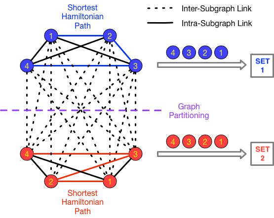
Figure 2. Graph optimization illustration to optimize convolution order of kernels.

1Given: A set of convolution kernels $V$ within a layer, and $K$ partitions required

2 Output: $K$ sets of optimized order of kernels where each set has size $|V|/K$

3 Construct a graph $G(V,E,W)$ where $w(v_{i},v_{j})=\#\text{Params}^{\text{Diff}}_{i,j}/\#\text{Params}_{i,j}$ (dissimilarity);

4 Partition $G$ into $K$ subgraphs by maximizing $\sum_{e_{ij}\in\text{inter-subgraph-links}}w(v_{i},v_{j})$, each denoted as $G_{k},k=1,...,K$;

5 for each $G_{k}$ do

6       Find the shortest Hamiltonian Path $H_{k}$ in $G_{k}$;

7      

8 end for

9Return: $K$ sets of optimized kernel order as $\left\{H_{k},k=1,2,...,K\right\}$;

Algorithm 1 Weight Reuse Optimization

Although regular weight reuse can accelerate BNN inference reasonably, we find that it is possible to optimize the weight reuse by re-ordering the convolution on kernels in each layer. In other words, the default computation order of kernels may not be good enough. Here we develop an algorithm to find a better order of convolutions using graph optimization. As shown in Fig. 2, we build a graph $G(V,E,W)$ where each vertex $v\in V$ corresponds to one kernel. Two vertices are connected by link $e\in E$ with weight $w\in W$ where $w$ represents degree of dissimilarity between two kernels. To find the optimal order of convolutions, we need to search for the scheduling where the total dissimilarity is minimized, i.e., total similarity is maximized.

3.3.1. Graph Partitioning.

We first partition the graph into several subgraphs. The reason is that our proposed architecture has limitations on the number of kernels for reverting in each computation unit (i.e., Set 1 and 2 in Fig. 2). Suppose there we partitioned all the kernels into $K$ subset, then each computation unit will work on $|V|/K$ kernels. To partition the original graph into $K$ subgraphs, we maximize the summed weight of links in between subgraphs. In other words, we maximize the dissimilarity in between group of kernels so that similarity is maximized within each group.

3.3.2. Sub-Graph Optimization.

For each subgraph containing $|V|/K$ vertices, we compute the shortest Hamiltonian path thus the accumulated dissimilarity is minimized along the path. Here we use a greedy approach to solve Hamiltonian path problem in an efficient way because the graph can be very large if there exists a lot of kernels within a layer (e.g., 1024), although non-greedy approach may be viable when the graph size is small, since this is optimized offline after BNN has been trained. The complete algorithm is shown in Algorithm 1.

After the above optimization, we can get the optimized order of convolution in terms of kernel indices for each computation unit. Then we will send this indexing map to the hardware in order to process it. In this design, in order to alleviate the hardware complexity and the overhead of the ofmaps reverting process, we put a limitation on $|V|/K$ to be 64. More complicated design to optimize partitions may be considered in future work.

4. Hardware Architecture

In this section, we introduce a hardware architecture that exploits the BNN similarity to save computations and memory accesses. Recall that we have two types of reuse strategies discussed in the above section and so we present two types of accelerators that leverage input and kernel similarity, respectively.

4.1. Input Reuse Accelerator

Figure 3. Block diagram of (a) input reuse accelerator and (b) weight reuse accelerator

The block diagram of the architecture that exploits the input similarity accelerator is shown in Figure 3 (a). For the input reuse accelerator, the execution has mainly three stages – data loading, computation, and accumulation. For the data loading stage, the input and weight data will be read from off-chip memory and be stored into the data buffer and weight memory banks (WBank). During the execution of a binarized convolution layer, the input data will be read from one data buffer and written to another equally size buffer. The read or write mode of data buffer A and B (Figure  3) will be switched for the computation of different layers so the input of each layer does not need to transfer back and forth between on-chip and off-chip memory.

During the computation stage, the entire system works in a producer and consumer fashion. The producer is the checking Engine (Chk) which is implemented as a bitwise C-by-C subtraction logic for checking the current input versus the previous one. For the computation of the first input during computation stage, which is corresponding to the STAGE I discussed in Section  3.2, Chk will broadcast the original input value and the Processing Elements (PE) will compute the result in the traditional way by using XNOR and popcount. For the rest of the input, we will use the reuse method for the computation, which is consistent with STAGE II mentioned in Section  3.2. During the reuse computation, Chk subtracts the current input with the previous one to check the difference. Once the checking is failed, the Chk will broadcast the subtraction result to all the PEs through a broadcasting bus. PE will read the weight out of the Wbank and scan the bus to find the different elements and update the reuse buffer which contains the result of last execution.

The different input values will be executed by $n$ different PEs simultaneously. Each PE is assigned with a reuse buffer, a Wbank, and an Output Activation bank (OAbank). The storage of weight is partitioned in kernel or $k$ dimensions, so that the ofmaps result will not interleave across different OAbanks. Once the current pixel has finished broadcasting, the accumulation stage will begin. The address generator and accumulator will collect the results in the reuse buffer and accumulate them into the corresponding position of OAbank.

4.1.1. Address Generator and Accumulator

The address generator calculates the destination address for different intermediate result in the reuse buffer. The OAbank accumulation controller will collect the result in reuse buffer and reduce them into the correct positions in OAbank which indicates by the address generator. The address of the ofmap $(h_{o},w_{o},c_{o})$ (subscript $o$ denotes output) of the given input locating at $(h,w,c)$ and weight locating at $(r,s,c,k)$ can be calculated as $(h-r,w-s,k)$ or $(h-r+1,w-s+1,k)$ if padding mode is enabled.

4.1.2. Batch Normalization Engine

Once the computation of the current layer is finished, the batch normalization engine will concatenate the ofmaps results from different OAbanks and normalize the output by subtracting the normalization factor before binarizing the value into -1/+1. Our strategy of doing batch normalization and pooling is similar to previous BNN acceleration work like (Umuroglu et al., 2017)(Zhao et al., 2017). Batch-normalization and activation functions are done together by comparing to the normalization factors across different ofmaps computed offline and then the pooling is done by using lightweight boolean AND operator. The entire batch normalization engine in our design for input similarity accelerator consumes 1541LUT and 432FF for a PE size of 8.

4.2. Weight Reuse Accelerator

For the weight reuse accelerator, the architecture is very similar to the input reuse accelerator. First, as is shown in Figure 3 (b), different lines of the input activation (IA) will be evenly distributed across PEs instead of different weight kernels for input reuse accelerators. But still, two equally-sized buffers will be assigned to each PE. The IA data will be read from and written into two separate buffers as the input reuse accelerator. Second, instead of broadcasting the input difference to PE like the input reuse accelerators, weight reuse accelerator broadcasts the difference between the weight kernels to PE.

We first pre-process the weights off-line by using the algorithm introduced in Section 3.3 to reorder the weight kernels with different $k$ dimensions to produce similarity. The hardware allows the weight kernel to be executed out-of-order in a given re-ordering range as we will revert the sequence of the ofmaps on-chip. Larger reordering range can achieve even higher degrees of similarity among weight kernels but also introduces higher ofmap reverting overhead. The sequence information of the permuted weight kernels needs to be loaded on-chip for reverting the ofmaps. But overall, assuming the reordering range is 64, the sequence information overhead is 10K bits which is less than 0.2% of the size of the weight kernels and thus can be ignored.

We also replace the representation of -1/+1 in weight kernel with ”same” (0) and ”different” (1), except for the first dot product computation. In this way, the on-chip checking process can bypass the subtraction logic. Once the computation begins, the weights will be loaded into the weight buffer and the input activation will be distributed to the IA buffers on-chip. The checking engine does not need to do subtraction as the weights have been pre-processed off-line in the representation of in ”different” (1) versus ”same” (0). The first weight kernel to be computed will still use the original value with XNOR and popcount for accumulation. It will also be stored in the checking engine as a weight base which will be continuously updated during the checking process. The goal of the weight base is to keep the latest version of the real weight value to recover the weight difference during the computation. For the rest of the computations, we begin to use the weight reuse strategy for computation. The Chk will scan the weight value to check the similarity. Once the similarity check fails in the computation, the Chk will generate the weight difference based on the weight base vector and broadcast the weight difference to all the PEs where different lines of the input activation are stored. In the meanwhile, the Chk will update the weight base which is the real weight data used for the following computation.

The address generator is still used for the calculation of a uniform address for PE reduction once a weight kernel finishes broadcasting. As the input is not duplicated in different IA buffer, some results in OAbank are partial sums which need to be further reduced in the last stage before the batch normalization and pooling. The final batch normalization engine will finish the last reduction before the batch normalization and ofmap reverting process. The final result will be stored back into the data buffer once the execution is finished. Overall, the design of weight reuse acceleration is a symmetric version of input reuse accelerator where we exploit kernel similarity across different. The differences between input reuse and weight reuse accelerator are mainly in the reduction and reverting logic. More complicated design can achieve better parallelization which is left for future work.

5. Evaluation

In this section, we evaluate our proposed reuse strategies on a real FPGA board. The following results show increased performance by using our method compared with benchmark BNN model in terms of speed and energy efficiency.

5.1. Prototype Implementation

To evaluate our design, we implement two types of BNN inference accelerators which exploits input and weight reuse strategies respectively for convolutional layers (conv). The process of decision-making between input or weight reuse strategy depends on the performance of the two types of accelerators on a given model. We test the design on the BinaryNet – an inference model for CIFAR-10 (Krizhevsky and Hinton, 2009) ($32\times 32$ color images) classification. The pre-trained BinaryNet (Courbariaux and Bengio, 2016) neural network is from the open-source code of (Zhao et al., 2017). The summary of the workload is listed in Table  2. The BinaryNet for CIFAR-10 model can achieve $11.19\%$ testing error. Our design can also be used to accelerate BNN models other than BinaryNet with arbitrary weight kernel size.

The prototype is implemented by using high-level synthesize tool Xilinx SDx 2018.1. The accelerated functions are written in high-level programming language. The SDx synthesize tool can automatically generate essential AXI bus for memory communication between off-chip memory and FPGA. The SDx tool also synthesizes the marked function into RTL and bitstream. During the inference, the CPU will awake the FPGA acceleration once the hardware function is called. Our design is implemented on the Xilinx Zynq ZCU104 board containing an ARM Cortex-A53 processor with a target clock frequency of 200MHz. As our design is scalable in the number of PEs, we configure the design with 8 PEs in the following experiments.

Table 2. Summary of the workload

layer	input dim $(h,w)$	weight dim $(r,s,c,k)$	weight size (Bits)	graph partition parameters $(V,K)$
conv1	32,32	3,3,128,128	144K	64,2
pool	32,32	-	-	-
conv2	16,16	3,3,128,256	288K	64,4
conv3	16,16	3,3,256,256	576K	64,4
pool	16,16	-	-	-
conv4	8,8	3,3,256,512	1.1M	64,8
conv5	8,8	3,3,512,512	2.3M	64,8
pool	8,8	-	-	-

5.2. Performance Analysis

5.2.1. Sensitivity to input similarity

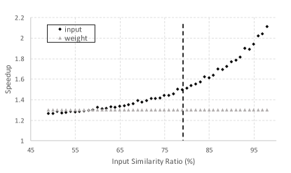
Figure 4. Performance of the accelerators as a function of the input and kernel similarity. The vertical dash line in the graph indicates the average input image similarity among the testing dataset. The baseline is the runtime of input reuse accelerator without using the reuse technique.

To show how we choose between the input and the weight reuse accelerator, we study the influence of input similarity ratio on the performance of the two designs. Figure 4 shows the speedup of accelerators as a function of the input similarity ratio defined in Section 3.3. The input reuse accelerator provides a variable speedup which depends on the similarity ratio of the input application. However, the weight reuse accelerator can provide a stable speedup which is based on the similarity ratio between weight kernels after re-ordering. As is shown by the vertical dash line in Figure 4, the speedup at the point of average input similarities of the input applications which is corresponding to the third row of Table  1, input reuse strategy can provide a better performance compared to weight reuse. Thus, we can conclude that for CIFAR-10 model, input reuse accelerator can provide a better performance and should be used for this BNN architecture. For BNN models with fixed-point input activations, as is shown in the 1 where the input is fixed-point value, the similarity ratio for input is low and the decision-making process may prefer weight reuse strategy in such case. The analysis for BNN models which prefer weight reuse is left for future work.

We also compare the performance of the input accelerator for different types of applications, ”rand” indicates the input image is random (-1/+1) series, while ”img” is the average performance of the testing images from CIFAR-10 testing dataset, ”max” is tested when all the pixels of the input image is in the same color, i.e., all the pixels in the classified input image are the same, ”w/o computation” indicates the runtime restricted by off-chip data transfer and CPU control overhead. Figure 5 shows the effect of these input applications versus speedup. For conv4 and conv5, the speedup of exploiting the input similarity is small and this is due to that the input activation size is small and weight size is large. We expect to see the bottleneck in these layers is in the off-chip memory bandwidth.

In terms of the speedup by weight reuse, we notice that the similarity ratio of kernel similarity cannot bring too much gain in the speedup. The detail of the speedup of weight re-ordering algorithm is shown in Figure  6. ”wt orig” indicates the performance of original weight order and ’wt re-order’ represents the performance of the acceleration applied with off-line reordered algorithm. By utilizing the re-ordering strategy, the inference can achieve 1.26 $\times$ speedup on average.

Figure 5. Speedup of the input similarity accelerator across different layers for different types of applications

To show the reduction in weight buffer access and the total number of operations by exploiting the BNN reuse technique, we study the reduction of weight buffer access and bitwise operations as is shown in Figure 7. The baseline is the weight buffer access and bit operations without using the input reuse technique. As the size of weights on-chip dominates the input activation size, we consider only the weight bank access in this experiment to approximate the total data buffer access in this analysis.

We observe that on average, the input reuse technique saves weight bank access by $40\%$ and bitwise operations by 80% for the testing images, which can lead to reduction in on-chip power consumption. The accelerator will bypass almost all the weight bank access and bitwise operations if the input application exhibits maximal similarity.

We can conclude that there is a high proportion of on-chip computation redundancy in BNN inference. And this property can be leveraged to reduce the on-chip power consumption and further accelerate the inference of BNN.

Table 3. Resource utilization and comparison to prior work.

	FPGA’16 (Qiu et al., 2016)	FPGA’16 (Suda et al., 2016)	FPGA’17(Zhao et al., 2017)	Our Design PE8	Our Design PE16
board	Zynq XC7Z045	Stratix-V GSD8	Zynq XC7Z020	Zynq XCZU7EV	Zynq XCZU7EV
clock(MHz)	150	120	147	200	200
precision (bit)	8-16	16	1-2	1-2	1-2
kLUTs	183	120*	46.9	45	72
FF	128K	no report	46K	13K	19K
DSPs	780	760*	3	5	1
BRAM	486	1377	94	112	1
GOPS (conv)	187.8	136.5	318.9	Rand 306.6 Img 411.4 Max 539.9	Rand 713.3 Img 917.7 Max 975.4
GOPS/kLUT	1.46	1.14	6.79	9.14	12.74
* refers to the approximation result from previous paper

Figure 6. Speedup of using the weight re-order algorithm. The baseline is the weight reuse architecture without using the reuse technique

Figure 7. Percentage of reduced weight bank access across different convolution layers

Figure 8. Percentage of reduced number of popcount across different convolution layers

5.3. Power Analysis

To further analyze the power savings in our accelerator, we study the power consumption which is measured at the socket by using a power monitor. The power consumption of programmable logic is calculated by subtracting the power measured while BNN is running with the power measured at idle stage. The measured results are averaged over a period of time while the accelerator is doing required inference.

Table 4. Power consumption of the programmable logic

	w/o reuse	w/o compute	img	max
Power (W)	0.36	0.21	0.30	0.23

Table 4 shows the power consumption of the programmable logic when FPGA is inferencing three different types of applications which are described above in Section  5.2. We also added a comparison column which shows the power consumption of data transfer without any on-chip computation. We can conclude that the input reuse strategy on average can reduce the total power consumption by $17\%$ and on-chip power consumption by $54\%$ compared to the baseline accelerator without exploiting the similarity reuse technique.

5.4. Comparison with Prior Work

We also compared our results with the state-of-the-art BNN design as shown in 3. As we focused on light-weight architecture for BNN acceleration, we choose a baseline with similar resource consumption for comparison and both of our architectures are for single-bit input and weight. We also put the result with floating point CNN accelerator  (Qiu et al., 2016) and  (Suda et al., 2016) here.

Our design is scalable with configurable number of PE. With a large amount of PEs, the on-chip computation will mostly be restricted by the memory bandwidth, the average giga-operations-per-second (GOPS) for testing image becomes closer to the ”max” GOPS when we scale the PE size to 16. Our result shows that with PE size of 8 and 16, the design achieves the 9.14 and 12.74GOPS/kLUT, which are 1.34$\times$ and 1.87$\times$ more area-efficient compared to our baseline. The power result is not fair to compare as our FPGA platform of implementation is not the same.

6. Related works

Binarized Neural Network: People have found that it is unnecessary to use floating weights and activations while preserving the accuracy of a neural network. The first approach is to use low-bitwidth fix-point numbers to approximate real values, which is called Quantized Neural Network (QNN) (Hubara et al., 2016). However, they cannot fully speed it up because we still need to live with costly operations on multiple bits.

Binarized Neural Network (BNN) was originally proposed in (Courbariaux et al., 2016) and has received a lot of attention in the research community since bit operations are fast and energy efficient compared to floating-point operations. They have shown the advantage of BNNs in terms of speed, memory usage and power consumption compared with traditional floating number CNN. Many recent works have been proposed to cure BNN’s optimization problem during training (Rastegari et al., 2016; Zhou et al., 2016; Courbariaux and Bengio, 2016). Recently people use ensemble strategy to build a strong binarized network to make BNN both accurate and robust (Zhu et al., 2018). In this work, we mainly focus on further accelerating BNN inference on FPGA, and our method can be applied to any state-of-the-art BNN architectures.

FPGA acceleration for CNN: FPGA acceleration of CNNs is gaining increasing attention due to the promising performance and cost efficiency. For instance, Zeng et al. (Zeng et al., 2018) proposed to employ frequency domain technique to accelerate floating point CNN. Escher et al. (Shen et al., 2017) proposed a design that accelerates CNN by optimizing the on-chip storage through identifying optimal batch size for CNNs. Previous work (Li et al., 2016) proposed a layer pipelined structure for accelerating large-scale CNN. Ma et al. (Ma et al., 2016) proposed a compiler design for a scalable RTL to accelerate CNN. Qiu et al. (Qiu et al., 2016) adopted singular values decomposition to reduce fully-connected layer bandwidth restriction. A recent study (Zhang et al., 2016) develops a uniform matrix multiplication to accelerate CNNs. Zhang et al. (Zhang et al., 2015) proposed the roofline model which illustrate the computation and memory bond for CNN acceleration and used the model to find the best configuration acceleration.

FPGA acceleration for BNN: Several recent studies explore FPGA acceleration of BNNs. FINN (Umuroglu et al., 2017) resolved the memory bond issue by storing all the parameters on-chip. Nakahara et al. (Nakahara et al., 2018) presented a modified BNN version of YOLOv2 to perform real-time localization and classification.  (Liang et al., 2018a) proposed a Resource-Aware Model for optimizing on-chip resource by quantized some part of the input activation. Kim et al. (Kim et al., 2017) proposed a kernel decomposition method for BNNs to reduce computation by half.

Li et al. (Li et al., 2017) developed an FPGA-based BNN accelerator by leveraging the look-up table (LUT) resources on FPGAs. In order to efficiently implement the normalization and binarization in BNNs with FPGA’s LUTs, the design merges the two into a single comparison operation. The study also performs a design space exploration in order to model throughput to improve acceleration performance. Although the design optimizes computation resource utilization by LUT-based computation, the performance is still susceptible to data access bottlenecks (Zhang et al., 2015).

ASIC acceleration for BNN: XNORBIN (Bahou et al., 2018) and Conti et al. (Conti et al., 2018) implemented Application-specific integrated circuit (ASIC) based BNN accelerators. Their designs adopted loop unrolling and data reuse to exploit the inherent parallelism of BNNs. However, the design simply maps BNN algorithms onto hardware. As a result, their performance improved over traditional neural network accelerations implementations is due to the efficiency of native BNN algorithms. YodaNN  (Andri et al., 2016) and BRein Memory  (Ando et al., 2018) are proposed ASIC accelerators for accelerating BNN inference.

Computation reuse for CNN: Computation reuse strategies have been proposed for DNN. Marc et al.  (Marc Riera, 2018) exploits input similarity between frames to reduce the computation of fixed point DNN inference. The reuse strategy quantizes the input first before checking the value with previous input. Thus, the method will sacrifice a little bit of classification precision. UCNN  (Hegde et al., 2018) quantizes the weight by using TTQ (or INQ) strategy, so only 3 (or 17) possible values of weight are available in the network. They sort the weights off-line based on weight values to factorize dot product and reduce computation power consumption.

These prior works on BNN and FPGA, ASIC for accelerating CNNs have enlightened the path of developing high-performance and energy-efficient neural network acceleration. To our knowledge, this is the first paper to exploit similarity in kernels and input activations to effectively accelerate BNNs on FPGA.

7. Discussion

Comparison between input and weight reuse: In this paper, we show better performance in speed and energy by using the two types of reuse strategies, i.e., input and weight reuse. From Table  1, we also notice their differences in different datasets and network models. Generally speaking, the input activation binarization is causing much more harm to performance over weight binarization in BNN, and many high-performance BNNs still prefer using floating or quantized input (Zhou et al., 2016). In such case, weight reuse seems to be a better strategy since it can guarantee a higher degree of similarity. But for BNN where input activation is binarized as well (Rastegari et al., 2016), input reuse is highly preferred for most image classification tasks. We believe more exploration can be made on smartly switching these two strategies and also studying whether the acceleration variance would cause problems in real-time applications or not.

Combination of both reuse strategies: Another important perspective brought by this paper is to study the mixing architecture which combines these two reuse strategies together in order to gain advantages from both. There may be extra overhead to realize this combination since the hardware architecture could be different. One of the promising next step is to design a more complicated architecture on FPGA that can efficiently accelerate inference by maximizing total similarities.

Improving current inference architecture: The ideal architecture to reduce computation redundancy should decrease the number of $Ops\_per\_image$ in Equation  3 without affecting the Utilization. Our proof-of-concept architecture is constrained by the off-chip memory bandwidth under some circumstances. Besides, the control overhead for the reduction must also be considered. This results in a small gap between the performance of our accelerator without using the reuse strategy and the-state-of-the-art design. In our future work, we will exploit the similarity without affecting the utilization of multipliers. It is also possible to combine the input or weight reuse strategy with some previous BNN acceleration techniques  (Umuroglu et al., 2017), for example, storing all the weights on-chip for resolving the memory issue. In addition, the design should remain in low control overhead which saves on-chip resource for more computation units.

8. Conclusions

In this paper, we propose a new FPGA-based BNN acceleration scheme, which incorporates both algorithm and hardware architecture design principles. Our design focuses on reducing latency and power consumption of BNNs by exploiting input and kernel similarities. We have shown that BNN inference has the property of high ratio of similarity in both input and kernel weights. The similarity of the input image comes from the spatial continuity between input pixels. Kernel similarity can be enhanced by applying to a proposed reordering algorithm. With different fixed-point representation for BNN input activation, either input or weight exhibits higher similarity ratio which can be exploited to reduce the bit operations and buffer access. By leveraging these two properties of the BNN, we proposed two types of accelerators, which can be applied to different situations. We also summarized the insights generated by comparing these two accelerators to assist strategy selection and combination. Our experiment shows that the power and speed of BNN inference can be largely improved through reducing computation redundancy. We believe this work makes an important step towards deploying neural networks to real-time applications.

References

- (1)
- Ando et al. (2018) K. Ando, K. Ueyoshi, K. Orimo, H. Yonekawa, S. Sato, H. Nakahara, S. Takamaeda-Yamazaki, M. Ikebe, T. Asai, T. Kuroda, and M. Motomura. 2018. BRein Memory: A Single-Chip Binary/Ternary Reconfigurable in-Memory Deep Neural Network Accelerator Achieving 1.4 TOPS at 0.6 W. IEEE Journal of Solid-State Circuits 53, 4 (April 2018), 983–994. https://doi.org/10.1109/JSSC.2017.2778702
- Andri et al. (2016) R. Andri, L. Cavigelli, D. Rossi, and L. Benini. 2016. YodaNN: An Ultra-Low Power Convolutional Neural Network Accelerator Based on Binary Weights. In 2016 IEEE Computer Society Annual Symposium on VLSI (ISVLSI). 236–241. https://doi.org/10.1109/ISVLSI.2016.111
- Bahou et al. (2018) Andrawes Al Bahou, Geethan Karunaratne, Renzo Andri, Lukas Cavigelli, and Luca Benini. 2018. XNORBIN: A 95 TOp/s/W Hardware Accelerator for Binary Convolutional Neural Networks. CoRR abs/1803.05849 (2018). arXiv:1803.05849 http://arxiv.org/abs/1803.05849
- Chen et al. (2016) Y. Chen, J. Emer, and V. Sze. 2016. Eyeriss: A Spatial Architecture for Energy-Efficient Dataflow for Convolutional Neural Networks. In 2016 ACM/IEEE 43rd Annual International Symposium on Computer Architecture (ISCA). 367–379.
- Conti et al. (2018) F. Conti, P. D. Schiavone, and L. Benini. 2018. XNOR Neural Engine: a Hardware Accelerator IP for 21.6 fJ/op Binary Neural Network Inference. IEEE Transactions on Computer-Aided Design of Integrated Circuits and Systems (2018), 1–1. https://doi.org/10.1109/TCAD.2018.2857019
- Courbariaux and Bengio (2016) Matthieu Courbariaux and Yoshua Bengio. 2016. BinaryNet: Training Deep Neural Networks with Weights and Activations Constrained to +1 or -1. CoRR abs/1602.02830 (2016). arXiv:1602.02830 http://arxiv.org/abs/1602.02830
- Courbariaux et al. (2015) Matthieu Courbariaux, Yoshua Bengio, and Jean-Pierre David. 2015. BinaryConnect: Training Deep Neural Networks with binary weights during propagations. CoRR abs/1511.00363 (2015). arXiv:1511.00363 http://arxiv.org/abs/1511.00363
- Courbariaux et al. (2016) Matthieu Courbariaux, Itay Hubara, Daniel Soudry, Ran El-Yaniv, and Yoshua Bengio. 2016. Binarized neural networks: Training deep neural networks with weights and activations constrained to+ 1 or-1. arXiv preprint arXiv:1602.02830 (2016).
- Han et al. (2017) Song Han, Junlong Kang, Huizi Mao, Yiming Hu, Xin Li, Yubin Li, Dongliang Xie, Hong Luo, Song Yao, Yu Wang, Huazhong Yang, and William (Bill) J. Dally. 2017. ESE: Efficient Speech Recognition Engine with Sparse LSTM on FPGA. In Proceedings of the 2017 ACM/SIGDA International Symposium on Field-Programmable Gate Arrays (FPGA ’17). ACM, New York, NY, USA, 75–84. https://doi.org/10.1145/3020078.3021745
- Hegde et al. (2018) Kartik Hegde, Jiyong Yu, Rohit Agrawal, Mengjia Yan, Michael Pellauer, and Christopher W Fletcher. 2018. UCNN: Exploiting Computational Reuse in Deep Neural Networks via Weight Repetition. ISCA’18 (2018).
- Hubara et al. (2016) Itay Hubara, Matthieu Courbariaux, Daniel Soudry, Ran El-Yaniv, and Yoshua Bengio. 2016. Quantized Neural Networks: Training Neural Networks with Low Precision Weights and Activations. CoRR abs/1609.07061 (2016). arXiv:1609.07061 http://arxiv.org/abs/1609.07061
- Jouppi et al. (2017) Norman P. Jouppi, Cliff Young, Nishant Patil, and David A. Patterson et al. 2017. In-Datacenter Performance Analysis of a Tensor Processing Unit. CoRR abs/1704.04760 (2017). arXiv:1704.04760 http://arxiv.org/abs/1704.04760
- Kim et al. (2017) Hyeonuk Kim, Jaehyeong Sim, Yeongjae Choi, and Lee-Sup Kim. 2017. A kernel decomposition architecture for binary-weight convolutional neural networks. In Proceedings of the 54th Annual Design Automation Conference 2017. ACM, 60.
- Krizhevsky and Hinton (2009) A. Krizhevsky and G. Hinton. 2009. Learning multiple layers of features from tiny images. Master’s thesis, Department of Computer Science, University of Toronto (2009).
- Li et al. (2016) Huimin Li, Xitian Fan, Li Jiao, Wei Cao, Xuegong Zhou, and Lingli Wang. 2016. A high performance FPGA-based accelerator for large-scale convolutional neural networks. In 2016 26th International Conference on Field Programmable Logic and Applications (FPL). 1–9. https://doi.org/10.1109/FPL.2016.7577308
- Li et al. (2017) Yixing Li, Zichuan Liu, Kai Xu, Hao Yu, and Fengbo Ren. 2017. A 7.663-TOPS 8.2-W Energy-efficient FPGA Accelerator for Binary Convolutional Neural Networks. In FPGA. 290–291.
- Liang et al. (2018a) Shuang Liang, Shouyi Yin, Leibo Liu, Wayne Luk, and Shaojun Wei. 2018a. FP-BNN. Neurocomput. 275, C (Jan. 2018), 1072–1086. https://doi.org/10.1016/j.neucom.2017.09.046
- Liang et al. (2018b) Shuang Liang, Shouyi Yin, Leibo Liu, Wayne Luk, and Shaojun Wei. 2018b. FP-BNN: Binarized neural network on FPGA. Neurocomputing 275 (2018), 1072–1086.
- Lin et al. (2013) Min Lin, Qiang Chen, and Shuicheng Yan. 2013. Network In Network. CoRR abs/1312.4400 (2013). arXiv:1312.4400 http://arxiv.org/abs/1312.4400
- Ma et al. (2016) Yufei Ma, N. Suda, Yu Cao, J. Seo, and S. Vrudhula. 2016. Scalable and modularized RTL compilation of Convolutional Neural Networks onto FPGA. In 2016 26th International Conference on Field Programmable Logic and Applications (FPL). 1–8. https://doi.org/10.1109/FPL.2016.7577356
- Marc Riera (2018) Antonio González Marc Riera, Jose Maria Arnau. 2018. Computation Reuse in DNNs by Exploiting Input Similarity. ISCA’18 (2018).
- Nakahara et al. (2018) Hiroki Nakahara, Haruyoshi Yonekawa, Tomoya Fujii, and Shimpei Sato. 2018. A Lightweight YOLOv2: A Binarized CNN with A Parallel Support Vector Regression for an FPGA. In Proceedings of the 2018 ACM/SIGDA International Symposium on Field-Programmable Gate Arrays (FPGA ’18). ACM, New York, NY, USA, 31–40. https://doi.org/10.1145/3174243.3174266
- NVIDIA Corporation (2007) NVIDIA Corporation. 2007. NVIDIA CUDA Compute Unified Device Architecture Programming Guide. NVIDIA Corporation.
- Qiu et al. (2016) Jiantao Qiu, Jie Wang, Song Yao, Kaiyuan Guo, Boxun Li, Erjin Zhou, Jincheng Yu, Tianqi Tang, Ningyi Xu, Sen Song, Yu Wang, and Huazhong Yang. 2016. Going Deeper with Embedded FPGA Platform for Convolutional Neural Network. In Proceedings of the 2016 ACM/SIGDA International Symposium on Field-Programmable Gate Arrays (FPGA ’16). ACM, New York, NY, USA, 26–35. https://doi.org/10.1145/2847263.2847265
- Rastegari et al. (2016) Mohammad Rastegari, Vicente Ordonez, Joseph Redmon, and Ali Farhadi. 2016. XNOR-Net: ImageNet Classification Using Binary Convolutional Neural Networks. CoRR abs/1603.05279 (2016). arXiv:1603.05279 http://arxiv.org/abs/1603.05279
- Sharma et al. (2018) H. Sharma, J. Park, N. Suda, L. Lai, B. Chau, V. Chandra, and H. Esmaeilzadeh. 2018. Bit Fusion: Bit-Level Dynamically Composable Architecture for Accelerating Deep Neural Network. In 2018 ACM/IEEE 45th Annual International Symposium on Computer Architecture (ISCA). 764–775. https://doi.org/10.1109/ISCA.2018.00069
- Shen et al. (2017) Y. Shen, M. Ferdman, and P. Milder. 2017. Escher: A CNN Accelerator with Flexible Buffering to Minimize Off-Chip Transfer. (April 2017), 93–100. https://doi.org/10.1109/FCCM.2017.47
- Sim et al. (2016) J. Sim, J. Park, M. Kim, D. Bae, Y. Choi, and L. Kim. 2016. 14.6 A 1.42 TOPS/W deep convolutional neural network recognition processor for intelligent IoE systems. In 2016 IEEE International Solid-State Circuits Conference (ISSCC). 264–265.
- Simonyan and Zisserman (2014) Karen Simonyan and Andrew Zisserman. 2014. Very Deep Convolutional Networks for Large-Scale Image Recognition. CoRR abs/1409.1556 (2014). arXiv:1409.1556 http://arxiv.org/abs/1409.1556
- Suda et al. (2016) Naveen Suda, Vikas Chandra, Ganesh Dasika, Abinash Mohanty, Yufei Ma, Sarma Vrudhula, Jae-sun Seo, and Yu Cao. 2016. Throughput-Optimized OpenCL-based FPGA Accelerator for Large-Scale Convolutional Neural Networks. In Proceedings of the 2016 ACM/SIGDA International Symposium on Field-Programmable Gate Arrays (FPGA ’16). ACM, New York, NY, USA, 16–25. https://doi.org/10.1145/2847263.2847276
- Umuroglu et al. (2017) Yaman Umuroglu, Nicholas J Fraser, Giulio Gambardella, Michaela Blott, Philip Leong, Magnus Jahre, and Kees Vissers. 2017. Finn: A framework for fast, scalable binarized neural network inference. In Proceedings of the 2017 ACM/SIGDA International Symposium on Field-Programmable Gate Arrays. ACM, 65–74.
- Zeng et al. (2018) Hanqing Zeng, Ren Chen, Chi Zhang, and Viktor Prasanna. 2018. A Framework for Generating High Throughput CNN Implementations on FPGAs. In Proceedings of the 2018 ACM/SIGDA International Symposium on Field-Programmable Gate Arrays (FPGA ’18). ACM, New York, NY, USA, 117–126. https://doi.org/10.1145/3174243.3174265
- Zhang et al. (2016) C. Zhang, Zhenman Fang, Peipei Zhou, Peichen Pan, and Jason Cong. 2016. Caffeine: Towards uniformed representation and acceleration for deep convolutional neural networks. In 2016 IEEE/ACM International Conference on Computer-Aided Design (ICCAD). 1–8. https://doi.org/10.1145/2966986.2967011
- Zhang et al. (2015) Chen Zhang, Peng Li, Guangyu Sun, Yijin Guan, Bingjun Xiao, and Jason Cong. 2015. Optimizing FPGA-based Accelerator Design for Deep Convolutional Neural Networks. In Proceedings of the 2015 ACM/SIGDA International Symposium on Field-Programmable Gate Arrays (FPGA ’15). ACM, New York, NY, USA, 161–170. https://doi.org/10.1145/2684746.2689060
- Zhao et al. (2017) Ritchie Zhao, Weinan Song, Wentao Zhang, Tianwei Xing, Jeng-Hau Lin, Mani Srivastava, Rajesh Gupta, and Zhiru Zhang. 2017. Accelerating binarized convolutional neural networks with software-programmable fpgas. In Proceedings of the 2017 ACM/SIGDA International Symposium on Field-Programmable Gate Arrays. ACM, 15–24.
- Zhou et al. (2017) Aojun Zhou, Anbang Yao, Yiwen Guo, Lin Xu, and Yurong Chen. 2017. Incremental Network Quantization: Towards Lossless CNNs with Low-Precision Weights. CoRR abs/1702.03044 (2017). arXiv:1702.03044 http://arxiv.org/abs/1702.03044
- Zhou et al. (2016) Shuchang Zhou, Yuxin Wu, Zekun Ni, Xinyu Zhou, He Wen, and Yuheng Zou. 2016. Dorefa-net: Training low bitwidth convolutional neural networks with low bitwidth gradients. arXiv preprint arXiv:1606.06160 (2016).
- Zhu et al. (2016) Chenzhuo Zhu, Song Han, Huizi Mao, and William J. Dally. 2016. Trained Ternary Quantization. CoRR abs/1612.01064 (2016). arXiv:1612.01064 http://arxiv.org/abs/1612.01064
- Zhu et al. (2018) Shilin Zhu, Xin Dong, and Hao Su. 2018. Binary Ensemble Neural Network: More Bits per Network or More Networks per Bit? arXiv preprint arXiv:1806.07550 (2018).