remarkRemark \newsiamremarkhypothesisHypothesis \newsiamthmclaimClaim \headersMaher Nouiehed, Jason Lee, and Meisam Razaviyayn \externaldocumentex_supplement
Convergence to Second-Order Stationarity for Constrained Non-Convex Optimization
Abstract
We consider the problem of finding an approximate second-order stationary point of a constrained non-convex optimization problem. We first show that, unlike the gradient descent method for unconstrained optimization, the vanilla projected gradient descent algorithm may converge to a strict saddle point even when there is only a single linear constraint. We then provide a hardness result by showing that checking -second order stationarity is NP-hard even in the presence of linear constraints. Despite our hardness result, we identify instances of the problem for which checking second order stationarity can be done efficiently. For such instances, we propose a dynamic second order Frank–Wolfe algorithm which converges to ()-second order stationary points in iterations. The proposed algorithm can be used in general constrained non-convex optimization as long as the constrained quadratic sub-problem can be solved efficiently.
1 Introduction
Designing efficient algorithms for non-convex optimization has recently been an active area of research, see [1, 6, 7, 8, 9, 10, 11, 14, 15, 30, 34]. For a general non-convex problem, even finding a local optimum of the objective function is in general NP-Hard [32]. Therefore, in practice, most existing algorithms converge to first or second order stationary points. The latter provides stronger guarantees as it constitutes a smaller subset of the critical points of the objective function that includes local and global optima. Moreover, when applied to functions with “nice” geometrical properties, the set of second order stationary points could even be the same as the set of global optima; see [2, 3, 5, 35, 39, 40, 41] for examples of such objective functions.
Most existing algorithms used for finding second order stationary points focus on unconstrained optimization problems. As a first order algorithm, [18] proposes a noisy-stochastic gradient descent method and shows convergence to the set of second-order stationary points, almost surely. Similarly, [28] uses stable manifold theorem to show that gradient descent with random initialization and sufficiently small constant step size converges to the latter set of second-order stationary points. More specifically, they show that the set of initial points that converge to a strict saddle point of the objective function is a measure zero set. Under the assumption that strict saddle property holds, the latter methods converge to a local optimum of the objective function. As a negative result, [17] constructs an example where the simple gradient descent can take exponential number of iterations to escape a strict saddle point. Motivated by this example, [24] proposes a perturbed form of gradient descent that can efficiently escape saddle points under strict saddle property.
Using higher order derivative information of the objective function, [7, 8, 15, 34, 37] propose trust region or cubic regularization methods for finding second order stationary points for unconstrained optimization problems. More specifically, the traditional trust region method [12, Algorithm 6.1.1] and cubic regularization methods, which are based on the work of [21, 34], are able to converge to second order stationary points. Moreover, [7, 8] proposed the Adaptive Regularization framework using Cubics, also known as (ARC), and established convergence to a second order stationary point. This method computes at each iteration an (approximate) global optimum for a local cubic model which resembles the behavior of the original objective function. They show that ARC requires iterations to converge to an -first-order stationary point, and iterations to reach an -second-order stationary point. Motivated by these rates, [15] designed a trust region method, entitled TRACE, which has the same iteration complexity bound as ARC. TRACE alters the acceptance criteria adopted in the traditional trust region method, and introduces a new mechanism for updating the radius of the trust region. In a more recent work, [13] developed an algorithm with a dynamic choice for direction and step-size. In particular, the dynamic algorithm decides on the step that offers a more significant predicted reduction in the objective value. The dynamic algorithm, ARC and TRACE methods fall under a more general framework that was proposed in [14]. This framework uses a set of generic conditions that need to be satisfied at each trial step, and converges to second order stationarity with optimal iteration complexity bound.
For constrained optimization problems, many recent papers propose algorithms that converge to first-order and second-order stationary points. For example, [26] proposed a Frank–Wolfe algorithm that converges to an -first order stationary point with complexity . Another work by [20] shows that projected gradient descent converges to an -first order stationary point with the same complexity bound. Convergence to second-order stationary points can be achieved by extending some of the aforementioned second or third order methods. For instance, [6] adapted the ARC method and showed that the worst-case function evaluation complexity for converging to an -first order stationary point is . Moreover, [10] showed that the same rate of convergence can be achieved for solving general smooth problems involving both non-convex equality and inequality constraints, using a cubic regularization method. In addition, a conceptual trust region method was proposed in [11] to compute an -approximate -th order stationary point in at most iterations. The iteration complexity bounds computed for these methods hide the per-iteration complexity of solving the sub-problem. These sub-problems are either quadratic or cubic constrained optimization problems, which are in general NP-complete; see section 4 in this paper.
Concurrent to this work, [31] proposed a general framework that yields convergence to an approximate -second order stationary point in at most iterations. This is achieved when the feasible set is convex and compact. In particular, the framework uses a first order method to converge to an approximate first order stationary point, and then computes a second order descent direction if it exists. However, as we show in Section 2, given any positive scalars and , the algorithm may converge to an approximate strict saddle point. More specifically, we provide a counterexample for which given any positive scalars applying the algorithm proposed in [31] finds an approximate strict saddle point. Since solving the quadratic sub-problem to optimality is NP-Hard, they suggest to approximately solve the sub-problems. In this paper, we show that, even for linear constraints, finding an approximate solution for these sub-problems is NP-Hard.
In addition to these second order methods, first order methods have also been used for finding second order stationary points of optimization problems with manifold constraints. The recent work [27] shows that manifold gradient descent converges to local minima under the strict saddle property. More recently, [22] established a similar result for a primal-dual optimization procedure implemented to solve linear equality constrained optimization problems. Unlike the linear equality constrained scheme, the convergence of first order algorithms to second-order stationarity is poorly understood in the presence of linear inequality constraints.
In this paper, we first provide an example that shows that projected gradient descent algorithm may converge to strict saddle points with positive probability even in the presence of a single linear constraint. We then discuss an NP-hardness result about solving the sub-problem of current second-order methods applied to constrained optimization problems. In addition, we provide a counterexample showing that current iterative second-order algorithms may get stuck near a strict saddle point. Motivated by this counterexample and inspired by the algorithms proposed in [13] and [26], we propose a second-order Frank–Wolfe algorithm that uses a dynamic choice for the direction and step-size. Moreover, our algorithm adopts a dynamic mechanism for escaping the region near strict saddle points that can be of independent interest. We show the algorithm converges to (-second order stationary points in iterations. Unlike the algorithms proposed in [26, 31], our algorithm does not require any boundedness assumption on the feasible set.
2 First and Second Order Stationarity
To understand the definitions of first and second order stationarity, we first consider the unconstrained optimization problem
| (1) |
where is a twice continuously differentiable function. We say a point is a first order stationary point of (1) if . Similarly, a point is said to be a second-order stationary point if and . Moreover, we say is a strict saddle point if it is a first-order stationary point but not a second-order stationary point. If all second order stationary points of the objective function are local optima, we say the function satisfies the strict saddle property. This property is satisfied in many practical objective functions; see [18, 25, 39, 40, 41]. In addition, if every local optima of the objective function is globally optimal, then finding the global optimum of the objective boils down to finding a second order stationary point; see [19, 29, 35, 38] for examples of such functions.
We now extend these definitions to the constrained optimization problem
| (2) |
where is a closed convex set. We say a point is a first order stationary point of (2) if for all , or equivalently if
| (3) |
Similarly, as defined in [4], we say a point is a second order stationary point of (2) if is a first order stationary point and
| (4) |
Moreover, we say that (2) satisfies the strict saddle property if every saddle point of the objective is not a second order stationary point. Notice that these definitions simplify to the corresponding unconstrained definitions when .
Motivated by (3) and (4), given a feasible point , we define the following first and second order stationarity measures
| (5) |
and
| (6) |
These optimality measures have been previously used in the literature [12, 6, 10, 36]. Notice that since is feasible, and . These optimality measures can be linked to the standard definitions in [4] by the following Lemma.
Lemma 2.1
If then
-
•
if and only if is a first order stationary point.
-
•
if and only if is a second order stationary point.
The above lemma motivates the following definition.
Definition 2.2
Approximate first and second order stationary points:
-
•
Given a positive scalar , a point is said to be an -first order stationary point of the optimization problem (2) if and .
-
•
Given positive scalars and , a point is said to be an -second order stationary point of the optimization problem (2) if , and .
For unconstrained optimization problems, -first order stationarity condition defined in 2.2 boils down to the classical condition . Similarly, -second order stationarity condition defined in 2.2 is equivalent to and . These are the standard definitions of approximate first and second order stationarity for unconstrained optimization [13, 15, 14, 34, 8].
Remark 2.3
As indicated in [36], there are two major differences between our definition of -second order stationarity and the definition used in [31]. Firstly, the definition used for approximate first and second order stationarity in [31] does not include the normalization constraints and in (5) and (6). Secondly, [31] uses the equality constraint in (6) instead of the inequality constraint . The significance of including the normalization constraints and using the inequality constraint are illustrated in [36].
Remark 2.4 (Continuity of )
While the continuity of was established in [6], to our knowledge, the question of whether is continuous remains unanswered. As a negative result, we provide a counterexample showing that is non-continuous. Consider the optimization problem
| (7) |
and the sequence of point
where and . Then,
Hence, as . Also,
where
As , one can easily check that the feasible set . Hence, . Moreover,
We have constructed a counterexample of a sequence of points , with . Therefore, is a non-continuous function. According to our definition 2.2, given any prescribed positive constants and and for sufficiently large , defined in our counterexample is an -second order stationary point. However, can be arbitrarily close to which is a first order stationary point but not a second-order stationary point. The former undesirable scenario can occur in practice when using the algorithm proposed in [31]. More specifically, applying the algorithm proposed in [31] to minimize the function (7) with initial point finds a point near the origin which is a first but not second order stationary point. To avoid the former undesirable scenario, we have to show that if the sequence of iterates computed by the algorithm and , then . We propose an algorithm with this former property in Section 5.
In the unconstrained scenario, it is well-known that gradient descent with random initialization converges to second order stationary points with probability one [28]. Moreover, there exist various efficient algorithms for finding an -second order stationary point of the objective function [34, 15, 13, 14, 7, 8]. In what follows, we study whether these results can be directly extended to the constrained scenario by answering the following questions:
Question 1: Does projected gradient descent with random initialization converge to second order stationary points with probability one? Question 2: Does there exist an efficient algorithm for finding an -second order stationary point of the general constrained optimization problem (2)?
3 Projected Gradient Descent with Random Initialization May Converge to Strict Saddle Points with Positive Probability
It is known that gradient descent with fixed step size can converge to an -first order stationary point in iterations for unconstrained smooth optimization problems [33]. Moreover, with random initialization, this method escapes strict saddle points for general smooth unconstrained optimization problems with probability one [28]. In the general constrained optimization problem (2), projected gradient descent algorithm is a natural replacement for gradient descent. The iterates of the projected gradient descent algorithm are obtained by
where is the step-size, is the iteration number, and is the projection operator onto the feasible set . A natural question about projected gradient descent is whether it has the same behavior as the
gradient descent algorithm. More specifically, can projected gradient descent escape strict saddle points? To answer this question, we provide an example where projected gradient descent fails to converge to second order stationary points even in the presence of a single linear constraint.
Consider the following optimization problem:
| (8) |
The landscape of the function and its corresponding negative gradient mapping are plotted in Figures 1a and 1b. Notice that the function has the following first and second order derivatives:

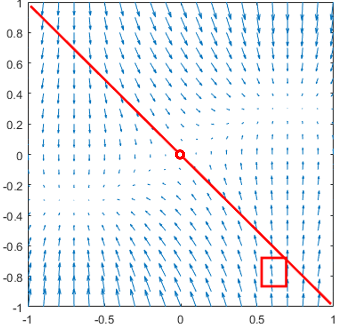
First of all, it is not hard to check that , , and for the feasible direction , we have . Hence, the point is a saddle point that is not second order stationary. Therefore, the origin is a strict saddle point. However, as one can see in Figure 1b, projected gradient descent algorithm may converge to the origin if initialized around the lower right corner of the figure. This observation is true for various step-size selection rules. To formalize this observation, in what follows, we show that projected gradient descent converges to the strict saddle point if initialized inside the red box in Figure 1b.
First, we show that if the sequence generated by projected gradient descent method intersects a subset of the boundary of the constraint in (8), then the algorithm will eventually converge to the origin.
Lemma 3.1
If for any , the iterate of the sequence generated by projected gradient descent method with constant step-size with applied to (8) satisfies
| (9) |
then converges to the origin.
Proof 3.2
Proof of this lemma is relegated to Appendix A.
It remains to show that there exists a non-zero measure region so that if we initialize the projected gradient descent algorithm in this region, the iterates converge to a point on the boundary satisfying the conditions in Lemma 3.1.
Theorem 3.3
For any given constant step-size with , there exists so that if we initialize in the set
then the projected gradient descent method with fixed step-size converges to the origin when applied to (8).
Proof 3.4
Proof of this Theorem is relegated to Appendix B.
This result shows that there is a positive probability that projected gradient descent with random initialization converges to a strict saddle point of the objective. Based on our example, we conjecture that even perturbed/stochastic projected gradient descent algorithm cannot help in escaping strict saddle points. Therefore, a natural question to ask is whether there exists a polynomial-time algorithm for finding an (approximate) second order stationary point. This question is the focus of the next section.
4 Finding or Checking (Approximate) Second Order Stationarity is NP-Hard Even in the Presence of Linear Constraints
The classical result of [32] shows that checking whether a point is a second-order stationary point of a non-convex quadratic optimization problem is in general NP-hard. This results was shown by considering the quadratic co-positivity problem
| (10) |
In particular, [32, Lemma 2] shows that, by adding a ball constraint , the optimal objective value of (10) is either or . Thus, checking whether is an -second order stationary point requires choosing . In that case [32, Theorem 2] shows that the problem is NP-Hard. Combining these two results, we conclude that checking whether is an -second order stationary point is NP-hard in . In this section, we show that even a less ambitious goal is NP-hard. More precisely, we show that checking -second order stationarity is NP-hard in .
Before proceeding to the result, let us define some notations. Let be a graph with the set of vertices and the set of edges . Also let be the cardinality of and be the adjacency matrix of graph . We define to be the set of co-positive matrices. We denote the all-one matrix of size by . We say graph has a stable set of size if it contains a subset of vertices, from which no two vertices in the subset are connected by an edge.
Lemma 4.1
Let be a graph with . Given a scalar with , define
Then the following are equivalent:
-
i.
-
ii.
contains a stable set of size
Proof 4.2
We first show that implies . By the definition of the set , the condition
implies that . Therefore, by [16, Lemma 4.1], contains a stable set of size .
To show the converse, we use [16, lemma 4.5]. Suppose that contains a stable set of size . By [16, lemma 4.1], . Moreover, by [16, lemma 4.5] it is far away from . In other words, there exists a such that
| (11) |
Let . If , we can clearly scale and reduce the objective value. Hence, . We now define,
By (11), we get that . If
| (12) |
then we have,
where the third equality holds by (12). This directly implies .
To complete the proof, we still need to show that
Assume the contrary, then we can define to be the minimizer
By the same previous argument, . Hence,
where the first and last equalities hold since , and the inequality holds by definition of . Hence, is not an optimal solution for
thus arriving to a contradiction.
The result of the above lemma directly implies the following theorem about the hardness of checking second order stationarity.
Theorem 4.3
For the co-positivity problem
| (13) |
there is no algorithm which can check whether is an -second order stationary point in polynomial time in , unless P = NP.
Proof 4.4
The resultt is an immediate consequence of Lemma 4.1.
Remark 4.5
The result in [32] shows that checking for -second order stationarity is NP-hard in . In other words, there is no algorithm which can check whether is an -second order stationarity point in polynomial time in , unless P=NP. The result of Theorem 4.3 is stronger as it shows that checking for -second order stationarity is NP-hard in .
This negative result shows that we should not expect to have a polynomial-time iterative descent algorithm which can converge to second order stationary points of general convex constrained optimization problems. If such an algorithm exists, one can run that algorithm from the initial point and see if it can find a point with negative objective value. This observation shows that in order to have a reasonable descent algorithm (with polynomial per-iteration complexity), we must put the general convex constrained case behind; and develop algorithms for special type of constraints. This transition is the focus of the next section.
5 Easy Instances of Finding Second Order Stationarity in Constrained Optimization: A Second Order Frank-Wolfe Algorithm
As discussed in previous sections, although designing polynomial time algorithms for finding second order stationary points is easy when the optimization problem is unconstrained, the same problem becomes very hard in the general convex constrained case. In particular, even for checking second order stationarity, one needs to (approximately) solve a quadratic constrained optimization problem (6), which is NP-hard as shown in Section 4. However, for some special constraint sets , the quadratic constrained optimization problem (6) can be solved efficiently. For example, when is formed by a fixed number of linear constraints, [23] presents a backtracking approach which can find the solution of (6) in polynomial-time. More precisely, by doing an exhaustive backtracking search on the set of constraints, one can find the solution of the problem
| (14) |
in polynomial-time when assuming that is small and one can afford a search which is exponentially large in .
Assuming that (14) can be solved efficiently for a given , a natural question to ask is as follows:
Assume that the constraint set is such that the quadratic optimization problem (14) can be solved efficiently. For such a constraint set , can we find an -second order stationary point of the general smooth optimization problem (2) efficiently?
In this section, we answer this question affirmatively by proposing a polynomial time algorithm for finding an second order stationary point of problem (2) assuming that a quadratic optimization problem of the form (14) can be solved efficiently at each iteration. The proposed algorithm can be viewed as a simple second order generalization of the Frank-Wolfe algorithm proposed in [26]. In particular, in addition to the first order Frank-Wolfe direction computed by solving (5) at , we also compute a second-order descent direction by solving (6) at each iteration. Then we dynamically choose the direction that potentially offers a more significant predicted reduction in the objective value. This dynamic method was used in [13] to design an algorithm for unconstrained optimization problems. They show convergence to -second-order stationary points with complexity . Our proposed algorithm adapts this method to the constrained scenario while maintaining the same convergence guarantees and complexity bounds.
Notations. Given a sequence of iterates computed by an algorithm for solving (2), we define where is defined in (5). Moreover, we define
| (15) |
where is positive scalar dynamically updated by the algorithm.
Throughout this section, we make the following standard assumptions.
Assumption 5.1
The objective function is twice continuously differentiable and bounded below by a scalar on . The constraint set is closed and convex. We assume that functions and are Lipschitz continuous with Lipschitz constants and , respectively. Furthermore, the gradient sequence is bounded such that there exists a scalar constant such that for all . Moreover, we assume that the Hessian sequence is bounded in norm, that is, there exists a scalar constant such that for all .
Moreover, we make the following assumption.
Assumption 5.2
There exists a constant such that if satisfies , then either or .
In simpler words, we assume that every first-order stationary point is either a second-order stationary point or has a feasible negative curvature direction satisfying . In the unconstrained scheme, this assumption implies that the absolute value of the smallest negative eigenvalue among all strict saddle points is bounded away from zero. If the smallest negative eigenvalue among strict saddle points can be arbitrarily close to zero, then given any prescribed positive constants and , an approximate strict saddle point can be confused with approximate second-order stationary points. Even in the case of first-order stationarity, if the norm of the gradient of non-critical points can be arbitrarily close to zero, then given any prescribed positive constant , iterative first-order algorithms can get stuck at these points. Next, we describe our proposed algorithm.
5.1 Algorithm Description
Let be the iterate in our algorithm at iteration . Given point , we define the following first order and second order descent directions
| (16) |
and
| (17) |
where is a positive scalar. Notice that in the unconstrained scenario, and is a feasible negative curvature direction. When , become the eigenvector corresponding to the leftmost eigenvalue of the Hessian matrix , which lead to the simple directions proposed in [13] for the unconstrained scenario.
The algorithm described below follows a dynamic strategy of choosing between and for all . The choice is done based on which direction predicts a larger reduction in the objective. If is always chosen, then the algorithm resembles Frank-Wolfe algorithm [26]. Hence, our algorithm can be seen as a second order extension of Frank-Wolfe algorithm. Moreover, the algorithm involves dynamic updates for the scalar . More specifically, the algorithm updates until the following conditions hold
| (18) |
where . The above conditions guarantee feasibility of next iterate and sufficient decrease in the objective value.
Require: , , , and .
5.2 Convergence Results
We first note that regardless of the direction we choose, the step size is either or , which by Cauchy Schwartz and conditions (18) are both less than or equal to . Thus, the iterates generated by the algorithm are always feasible. Also notice that, unlike the algorithms proposed in [26, 31], our algorithm does not require any boundedness assumption on the feasible set . Before proceeding to the proof of convergence of our algorithm, we first show the following essential Lemma.
Lemma 5.3
Proof 5.4
The proof is relegated to Appendix C.
The Lemma above indicates that if where is a strict saddle point, then there exists an such that is bounded below by a positive constant for all . Hence, if with and , then and for all . This is formally stated in the Corollary below.
Corollary 5.5
Consider a sequence of iterates generated by Algorithm 1 with . There exists such that if and . Then
for all .
Proof 5.6
By the continuity of [12], we get that . According to (20), we have
where is a monotone increasing function for with . Moreover, according to (19), we have
where is a monotone decreasing function for . Consider such that . By monotonicity of and , given , there exists with
and
Hence by definition of in 15, does not converge to zero which contradicts the assumption that . This completes the proof.
Theorem 5.7
Under Assumption 5.1,
In other words, any limit point of the iterates is a second order stationary point.
Proof 5.8
We start by showing that the algorithm exits the loop (Step 8) at every iteration . The claim is obvious when Step 9 tests True. We show that the claim holds when Step 9 tests False. Assume , then using second-order descent lemma [4] we obtain
| (21) |
where the fourth inequality holds since
Hence, if
| (22) |
conditions (18) are satisfied. This directly implies that Step 15 is reached and the algorithm exists the loop. We next show that (22) will be satisfied at every iteration . Assume the contrary, then
According to the definition of in (15),
| (23) |
where the first inequality holds since Step 9 tested False. By the update rule in Steps 17, . Therefore, and . However, if is not a second-order stationary point, which contradicts the convergence of to zero.
We have showed that (22) will be satisfied for every unless is a second-order stationary point. It follows that Step 15 or Step 11 is reached and the algorithm exists the loop. We next show that . To proceed with the proof, we show the following reduction bound in the objective value
Otherwise, Step 14 is reached and conditions (18) are satisfied. Hence, we get the following reduction bound in the objective value at every iteration
| (25) |
By summing over the iterations, we get
| (26) |
Hence, since is bounded below by , we have
Thus,
By Lemma 5.5, we get that every limit point of the iterates is a second order stationary point. This completes the proof.
The next result computes the worst-case complexity required to reach an -first order stationary point and to reach an -second order stationary point.
Theorem 5.9
Let , . The number of iterations required for Algorithm 1 to find an -first order stationary point is at most . Moreover, the number of iterations required to find an -second order stationary point is at most .
Proof 5.10
Let be the number of times Step 17 is reached. We first show .
Assume that
Then, by second-order descent lemma conditions (18) are satisfied which directly implies that Step 15 is reached and the algorithm exists the loop. Otherwise, if
then by the definition of we have
where the first inequality holds since Step 9 tested False.
It follows that
which implies that
| (27) |
Now define the index sets
Next we show bounds on and . First notice that the sufficient decrease bound (26) implies that
| (28) |
for every iteration . According to the bound (28), it is easy to show that the cardinality of the above two sets is bounded by
| (29) |
References
- [1] A. Anandkumar and R. Ge. Efficient approaches for escaping higher order saddle points in non-convex optimization. In Conference on Learning Theory, pages 81–102, 2016.
- [2] A. S. Bandeira, N. Boumal, and V. Voroninski. On the low-rank approach for semidefinite programs arising in synchronization and community detection. In Conference on Learning Theory, pages 361–382, 2016.
- [3] B. Barazandeh and M. Razaviyayn. On the behavior of the expectation-maximization algorithm for mixture models. arXiv preprint arXiv:1809.08705, 2018.
- [4] D. P. Bertsekas. Nonlinear programming. Athena scientific Belmont, 1999.
- [5] N. Boumal. Nonconvex phase synchronization. SIAM Journal on Optimization, 26(4):2355–2377, 2016.
- [6] C. Cartis, N. Gould, and P. L. Toint. An adaptive cubic regularization algorithm for nonconvex optimization with convex constraints and its function-evaluation complexity. IMA Journal of Numerical Analysis, 32(4):1662–1695, 2012.
- [7] C. Cartis, N. I. Gould, and P. L. Toint. Adaptive cubic regularisation methods for unconstrained optimization. part i: motivation, convergence and numerical results. Mathematical Programming, 127(2):245–295, 2011.
- [8] C. Cartis, N. I. Gould, and P. L. Toint. Adaptive cubic regularisation methods for unconstrained optimization. part ii: worst-case function-and derivative-evaluation complexity. Mathematical programming, 130(2):295–319, 2011.
- [9] C. Cartis, N. I. Gould, and P. L. Toint. On the evaluation complexity of cubic regularization methods for potentially rank-deficient nonlinear least-squares problems and its relevance to constrained nonlinear optimization. SIAM Journal on Optimization, 23(3):1553–1574, 2013.
- [10] C. Cartis, N. I. Gould, and P. L. Toint. On the evaluation complexity of constrained nonlinear least-squares and general constrained nonlinear optimization using second-order methods. SIAM Journal on Numerical Analysis, 53(2):836–851, 2015.
- [11] C. Cartis, N. I. Gould, and P. L. Toint. Second-order optimality and beyond: Characterization and evaluation complexity in convexly constrained nonlinear optimization. Foundations of Computational Mathematics, pages 1–35, 2017.
- [12] A. R. Conn, N. I. Gould, and P. L. Toint. Trust region methods, volume 1. Siam, 2000.
- [13] F. E. Curtis and D. P. Robinson. Exploiting negative curvature in deterministic and stochastic optimization. arXiv preprint arXiv:1703.00412, 2017.
- [14] F. E. Curtis, D. P. Robinson, and M. Samadi. An inexact regularized newton framework with a worst-case iteration complexity of o() for nonconvex optimization. arXiv preprint arXiv:1708.00475, 2017.
- [15] F. E. Curtis, D. P. Robinson, and M. Samadi. A trust region algorithm with a worst-case iteration complexity of o() for nonconvex optimization. Mathematical Programming, 162(1-2):1–32, 2017.
- [16] P. J. Dickinson and L. Gijben. On the computational complexity of membership problems for the completely positive cone and its dual. Computational optimization and applications, 57(2):403–415, 2014.
- [17] S. S. Du, C. Jin, J. D. Lee, M. I. Jordan, A. Singh, and B. Poczos. Gradient descent can take exponential time to escape saddle points. In Advances in Neural Information Processing Systems, pages 1067–1077, 2017.
- [18] R. Ge, F. Huang, C. Jin, and Y. Yuan. Escaping from saddle points—online stochastic gradient for tensor decomposition. In Conference on Learning Theory, pages 797–842, 2015.
- [19] R. Ge, J. D. Lee, and T. Ma. Matrix completion has no spurious local minimum. In Advances in Neural Information Processing Systems, pages 2973–2981, 2016.
- [20] S. Ghadimi, G. Lan, and H. Zhang. Mini-batch stochastic approximation methods for nonconvex stochastic composite optimization. Mathematical Programming, 155(1-2):267–305, 2016.
- [21] A. Griewank. The modification of newton’s method for unconstrained optimization by bounding cubic terms. Technical report, Technical report NA/12, 1981.
- [22] M. Hong, J. D. Lee, and M. Razaviyayn. Gradient primal-dual algorithm converges to second-order stationary solutions for nonconvex distributed optimization. arXiv preprint arXiv:1802.08941, 2018.
- [23] Y. Hsia and R.-L. Sheu. Trust region subproblem with a fixed number of additional linear inequality constraints has polynomial complexity. arXiv preprint arXiv:1312.1398, 2013.
- [24] C. Jin, R. Ge, P. Netrapalli, S. M. Kakade, and M. I. Jordan. How to escape saddle points efficiently. arXiv preprint arXiv:1703.00887, 2017.
- [25] K. Kawaguchi. Deep learning without poor local minima. In Advances in Neural Information Processing Systems, pages 586–594, 2016.
- [26] S. Lacoste-Julien. Convergence rate of frank-wolfe for non-convex objectives. arXiv preprint arXiv:1607.00345, 2016.
- [27] J. D. Lee, I. Panageas, G. Piliouras, M. Simchowitz, M. I. Jordan, and B. Recht. First-order methods almost always avoid saddle points. arXiv preprint arXiv:1710.07406, 2017.
- [28] J. D. Lee, M. Simchowitz, M. I. Jordan, and B. Recht. Gradient descent converges to minimizers. arXiv preprint arXiv:1602.04915, 2016.
- [29] H. Lu and K. Kawaguchi. Depth creates no bad local minima. arXiv preprint arXiv:1702.08580, 2017.
- [30] S. Lu, Z. Wei, and L. Li. A trust region algorithm with adaptive cubic regularization methods for nonsmooth convex minimization. Computational Optimization and Applications, 51(2):551–573, 2012.
- [31] A. Mokhtari, A. Ozdaglar, and A. Jadbabaie. Escaping saddle points in constrained optimization. arXiv preprint arXiv:1809.02162, 2018.
- [32] K. G. Murty and S. N. Kabadi. Some np-complete problems in quadratic and nonlinear programming. Mathematical programming, 39(2):117–129, 1987.
- [33] Y. Nesterov. Introductory lectures on convex optimization: A basic course, volume 87. Springer Science & Business Media, 2013.
- [34] Y. Nesterov and B. T. Polyak. Cubic regularization of newton method and its global performance. Mathematical Programming, 108(1):177–205, 2006.
- [35] M. Nouiehed and M. Razaviyayn. Learning deep models: Critical points and local openness. arXiv preprint arXiv:1803.02968, 2018.
- [36] M. Nouiehed and M. Razaviyayn. A trust region method for finding second-order stationarity in linearly constrained non-convex optimization. arXiv preprint arXiv:1904.06784, 2019.
- [37] C. W. Royer and S. J. Wright. Complexity analysis of second-order line-search algorithms for smooth nonconvex optimization. SIAM Journal on Optimization, 28(2):1448–1477, 2018.
- [38] J. Sun, Q. Qu, and J. Wright. When are nonconvex problems not scary? arXiv preprint arXiv:1510.06096, 2015.
- [39] J. Sun, Q. Qu, and J. Wright. A geometric analysis of phase retrieval. In Information Theory (ISIT), 2016 IEEE International Symposium on, pages 2379–2383. IEEE, 2016.
- [40] J. Sun, Q. Qu, and J. Wright. Complete dictionary recovery over the sphere i: Overview and the geometric picture. IEEE Transactions on Information Theory, 63(2):853–884, 2017.
- [41] J. Sun, Q. Qu, and J. Wright. Complete dictionary recovery over the sphere ii: Recovery by riemannian trust-region method. IEEE Transactions on Information Theory, 63(2):885–914, 2017.
Appendix A Proof of Lemma 3.1
For a given , let be the current iterate with . We first show that iterate generated by projected gradient descent satisfies
| (30) |
Then we show that
| (31) |
First note that if , then the result trivially holds. Assume that , we define
Since , the point is not feasible. By projecting to the feasible set , we obtain
| (32) |
Obviously (30) holds. We now show that
Let . This function has two global minima , and one global maximum . Hence,
| (33) |
Appendix B Proof of Theorem 3.3
Consider the initial point . If we can show that and , then using Lemma 3.1, we conclude that the sequence of iterates eventually converges to the origin. Thus it suffices to show that there exist an such that if
| (34) |
then the next iterate satisfies
| (35a) | |||
| (35b) | |||
The first condition (35a) is satisfied when the step-size is small enough. To prove (35b) we utilize the conditions in (34) to obtain the following inequalities
which implies that
| (36) |
Appendix C Proof of Lemma 5.3
Proof C.1
Consider satisfying and . By the convexity of , we get
Moreover, using Assumption 5.2, there exists such that
| (37) |
Case when :
| (38) |
where the first inequality holds by (37), Cauchy Shwartz, and -Lipschitzness of . The second inequality holds since and .
Case when :
| (39) |
where the second equality holds by our definition of , the first inequality holds by Cauchy Shwartz and the -Lipschitzness of , and the second inequality holds by (37) and since
Here since and by our choice of . Combining (38) and (39), we get that
Similarly, we show (20) by considering the following two cases.
Case when :
| (40) |
where the first inequality holds by Cauchy Shwartz and since . The second inequality holds by Assumption 5.2, -Lipschitzness of , and since .
Case when :
| (41) |
where the third equality holds by our definition of , and the first and second inequalities hold by Cauchy Shwartz, Assumption 5.1 and since . Here the third and fourth inequalities hold by -Lipschitzness of , Cauchy Shwartz and Assumption 5.2. Combining (40) and (41), we get that