A Comparison of I/O-Efficient Algorithms for Visibility Computation on Massive Grid Terrains

Abstract

Given a terrain $T$ and a viewpoint $v$, the visibility map or viewshed of $v$ is the set of grid points of $T$ that are visible from $v$. To decide whether a point $p$ is visible one needs to interpolate the elevation of the terrain along the line-of-sight (LOS) $vp$. Existing viewshed algorithms differ widely in what points they chose to interpolate, how many lines-of-sight they consider, and how they interpolate the terrain. These choices crucially affect the running time and accuracy of the algorithms. This paper describes I/O-efficient algorithms for computing visibility maps on massive grid terrains in a couple of different models.

First, we describe two algorithms that use the interpolation model of Van Kreveld. These algorithms sweep the terrain by rotating a ray around the viewpoint while maintaining the terrain profile along the ray. On a terrain of $n$ grid points, these algorithms run in $O(n\log n)$ time and $O(\mathsf{sort}(n))$ I/Os in the I/O-model of Aggarwal and Vitter. Second, we describe an algorithm which runs in $O(n)$ time and $O(\mathsf{scan}(n))$ I/Os, and is cache-oblivious. This algorithm sweeps the terrain centrifugally, growing a star-shaped region around the viewpoint while maintaining the approximate visible horizon of the terrain within the swept region.

Our last two algorithms use linear interpolation and the model of Franklin’s R3 algorithm, which in the literature is referred to as the “exact” algorithm. Our algorithms are based on computing and merging horizons, and we prove that the complexity of horizons on a grid of $n$ points with linear interpolation is $O(n)$, improving on the general $O(n\alpha(n))$ bound on triangulated terrains.

We present an experimental analysis of our algorithms on NASA SRTM data. All our algorithms are scalable to volumes of data that are over 50 times larger than main memory. Our main finding is that, in practice, horizons are significantly smaller than their theoretical worst case bound, which makes horizon-based approaches very fast. Our last two algorithms, which compute the most accurate viewshed, turn out to be very fast in practice, although their worst-case bound is inferior.

A preliminary version of this work appeared in Proceedings of the 17th ACM SIGSPATIAL Symp. of Geographic Information Systems (GIS 2009). Best-paper award, and in Proceedings of the 21st ACM SIGSPATIAL Symp. of Geographic Information Systems (GIS 2013).
Herman Haverkort, Department of Mathematics and Computer Science, Technische Universiteit Eindhoven, P.O. Box 513, 5600 MB Eindhoven, The Netherlands, cs.herman@haverkort.net.
Laura Toma, Department of Computer Science, Bowdoin College, 8650 College Station, Brunswick, ME 04011, USA, ltoma@bowdoin.edu.

1 Introduction

The computation of visibility is a fundamental problem on terrains and is at the core of many applications such as planning the placement of communication towers or watchtowers, planning of buildings such that they do not spoil anybody’s view, finding routes on which you can travel while seeing a lot or without being seen, and computing solar irradiation maps which can in turn be used in predicting vegetation cover. The basic problem is point-to-point visibility: Two points $a$ and $b$ on a terrain are visible to each other if the interior of their line-of-sight $ab$ (the line segment between $a$ and b) lies entirely above the terrain. Based on this one can define the viewshed: Given a terrain and an arbitrary (view)point $v$, not necessarily on the terrain, the visibility map or viewshed of $v$ is the set of all points in the terrain that are visible from $v$; see Figure 1. A variety of problems pertaining to visibility have been researched in computational geometry and computer graphics, as well as in geographic information science and geospatial engineering.

The key in defining and computing visibility is choosing a terrain model and an interpolation method. The most common terrain models are the grid and the TIN (triangular irregular network). A grid terrain is essentially a matrix of elevation values, representing elevations sampled from the terrain with a uniform grid; the x,y coordinates of the samples are not stored in a grid terrain, they are considered implicit w.r.t. to the corner of the grid. A TIN terrain consists of an irregular sample of points (x,y and elevation values), and a triangulation of these points is provided. Grid terrains are the most widely used in GIS because of their simplicity. Our algorithms in this paper discuss the computation of visibility maps on grid terrains.

To decide whether a point $p$ is visible on a given terrain model, one needs to interpolate the elevation along the line-of-sight $pv$ between the viewpoint $v$ and $p$ (more precisely, along the projection of the line-of-sight on the horizontal plane) and check whether the interpolated elevations are below the line of sight. Various algorithms differ in what and how many points they select to interpolate along the line-of-sight, and in the interpolation method used. These choices crucially affect the efficiency and accuracy of the algorithms.

In order to be useful in practice, viewshed algorithms need to be fast and scalable to very large terrains. The last decade witnessed an explosion in the availability of terrain data at better and better resolution. In 2002, for example, NASA’s Shuttle Radar Topography Mission (SRTM) acquired 30 m-resolution terrain data for the entire USA, in total approximately 10 terabytes of data. With more recent technology it is possible to acquire data at sub-meter resolution. This brings tremendous increases in the size of the datasets that need to be processed: Washington state at 1 m resolution, using 4 bytes for the elevation of each sample, would total 689 GiB of data; Ireland would be 262 GiB—only counting elevation samples on land. Data at this fine resolution has started to become available.

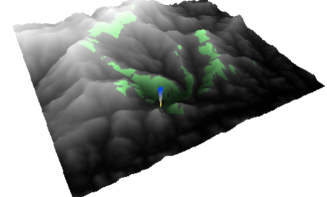
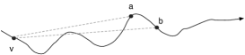
Figure 1: (a) The viewshed of a point on a grid terrain is shown in green. The viewpoint is marked in blue. (b) Two points on a terrain are visible to each other if the interior of their line-of-sight lies entirely above the terrain. Here $a$ is visible from $v$, but $b$ is not.

1.1 I/O-efficiency

Working with large terrains require efficient algorithms that scale well and are designed to minimize “I/O”: the swapping of data between main memory and disk. We assess the efficiency of algorithms in this paper not only by studying the number of computational steps they need and by measuring their running times in practical experiments, but also by studying how the number of I/O-operations grows with the input size. To this end we use the standard model defined by Aggarwal and Vitter [Aggarwal and Vitter (1988)]. In this model, a computer has a memory of size $M$ and a disk of unbounded size. The disk is divided into blocks of size $B$. Data is transferred between memory and disk by transferring complete blocks: transferring one block is called an “I/O”. Algorithms can only operate on data that is currently in main memory; to access the data in any block that is not in main memory, it first has to be copied from disk. If data in the block is modified, it has to be copied back to disk later, at the latest when it is evicted from memory to make room for another block. The I/O-efficiency of an algorithm can be assessed by analysing the number of I/Os it needs as a function of the input size $n$, the memory size $M$, and the block size $B$. The fundamental building blocks and bounds in the I/O-model are sorting and scanning: scanning $n$ consecutive records from disk takes $\mathsf{scan}(n)=\Theta(n/B)$ I/Os; sorting takes $\mathsf{sort}(n)=\Theta(\frac{n}{B}\log_{M/B}\frac{n}{B})$ I/Os in the worst case [Aggarwal and Vitter (1988)]. It is sometimes assumed that $M=\Omega(B^{2})$.

We distinguish cache-aware algorithms and cache-oblivious I/O-efficient algorithms: Cache-aware algorithms may use knowledge of $M$ and $B$, (and to some extent even control $B$) and they may use it to control which blocks are kept in memory and which blocks are evicted. Cache-oblivious algorithms, as defined by Frigo et al. [Frigo et al. (1999)], do not know $M$ and $B$ and cannot control which blocks are kept in memory: the caching policy is left to the hardware and the operating system. Nevertheless, cache-oblivious algorithms can often be designed and proven to be I/O-efficient [Frigo et al. (1999)]. The idea is to design the algorithm’s pattern of access to locations in files and temporary data structures such that effective caching is achieved by any reasonable general-purpose caching policy (such as least-recently-used replacement) for any values of $M$ and $B$. As a result, any bounds that can be proven on the I/O-efficiency of a cache-oblivious algorithm hold for any values of $M$ and $B$ simultaneously. Thus they do not only apply to the transfer of data between disk and main memory, but also to the transfer of data between main memory and the various levels of smaller caches. However, in practice, cache-oblivious algorithms cannot always match the performance of cache-aware algorithms that are tuned to specific values of $M$ and $B$ [Brodal et al. (2007)].

1.2 Problem definition

A terrain $T$ is a surface in three dimensions, such that any vertical line intersects $T$ in at most one point. The domain $D$ of $T$ is the projection of $T$ on a horizontal plane. The elevation angle of any point $q=(q_{x},q_{y},q_{z})$ with respect to a viewpoint $v=(v_{x},v_{y},v_{z})$ is defined as:

$$\textrm{ElevAngle}(q)=\arctan\frac{q_{z}-v_{z}}{\textrm{Dist}(q)},$$

where $\textrm{Dist}(q):=|(q_{x},q_{y})-(v_{x},v_{y})|$.

A point $u=(u_{x},u_{y},u_{z})$ is visible from $v$ if and only if the elevation angle of $u$ is higher than the elevation angle of any point of $T$ whose projection on the plane lies on the line segment from $(u_{x},u_{y})$ to $(v_{x},v_{y})$. We define the elevation angle of any point $(q_{x},q_{y})$ of $D$ as the elevation angle of the point $q=(q_{x},q_{y},q_{z})$ where the vertical line through $(q_{x},q_{y})$ intersects $T$.

In this paper we consider terrains that are represented by a set of $n$ points whose projections on $D$ form a regular rectangular grid. To decide whether a point $u$ is visible from a point $v$, we need to interpolate the elevation angle of points of $T$ whose projection on the plane lie along the line segment from $(u_{x},u_{y})$ to $(v_{x},v_{y})$.

We want to compute the following: given any terrain $T$ and any viewpoint $v=(v_{x},v_{y},v_{z})$, find which grid points of the terrain are visible to $v$ and which are not.

We assume the terrain is given as a matrix $Z$, stored row by row, where $Z_{ij}$ is the elevation of the point in row $i$ and column $j$. The output visibility map is a matrix $V$, stored row by row, in which $V_{ij}$ is $1$ if the point in row $i$ and column $j$ is visible, and $0$ otherwise.

For ease of presentation, throughout the rest of the paper we assume that the grid is square and has size $\sqrt{n}\cdot\sqrt{n}$ ; of course the actual implementations of our algorithms can handle rectangular grids as well.

1.3 Related work

The standard method for computing viewsheds on grid terrains is the algorithm R3 by Franklin and Ray [Franklin and Ray (1994)]. R3 determines the visibility of each point in the grid as follows: it computes the intersections between the horizontal projection of the line-of-sight and the horizontal and vertical grid lines, and computes the elevation of the terrain at these intersection points by linear interpolation. Since a line of sight intersects $O(\sqrt{n})$ grid lines, determining the visibility of a point takes $O(\sqrt{n})$ time. This is considered to be the standard model and R3 is considered to produce the “exact” viewshed [Izraelevitz (2003)]. However, as described by Franklin and Ray, R3 runs in $O(n\sqrt{n})$ time, which is too slow in practice, especially for multiple viewshed computations.

A variety of viewshed algorithms have been proposed that optimize R3 while approximating in some way the resulting viewshed: Some algorithms consider only a subset of the $O(n)$ lines-of-sight; others interpolate the line-of-sight only at a subset of the $O(\sqrt{n})$ intersection points with the grid lines; yet others have some other way of determining in $O(1)$ time whether a point in the grid is visible. The optimized viewshed algorithms run in $o(n\sqrt{n})$ time, most often $O(n)$. Examples are XDraw by Franklin and Ray [Franklin and Ray (1994)]; Backtrack by Izraelevitz [Izraelevitz (2003)]; R2 by Franklin and Ray [Franklin and Ray (1994)]; and van Kreveld’s radial sweep algorithm [van Kreveld (1996)]—below we describe briefly the results which are relevant to this paper.

The algorithm named R2, proposed by Franklin and Ray [Franklin and Ray (1994)], is an optimization of R3 that runs in $O(n)$ time. The idea of R2 is to examine the lines-of-sight only to the $O(\sqrt{n})$ grid points on the boundary of the grid; a grid point that is not on the boundary is considered to be visible if the nearest point of intersection between a grid line and one of the examined lines-of-sight is determined to be visible. Overall R2 is fast and, according to its authors, produces a good approximation of R3 that outweighs its loss in accuracy [Franklin and Ray (1994)].

The other algorithm, XDraw, computes the visibility of the grid points incrementally in concentric layers around the viewpoint, starting at the viewpoint and working its way outwards. For a grid point $v$ in layer $i$, the algorithm computes whether $v$ is visible, and what is the maximum height above the horizon along the line of sight to $v$. To do so, it determines which are the two grid points $q$ and $r$ in layer $i-1$ that are nearest to $\overline{pv}$, and then it estimates the maximum height above the horizon along $\overline{pv}$ by interpolating between the lines of sight to $q$ and $r$. Thus, the visibility of each point is determined in constant time per point. XDraw is faster than R3 and R2, due to the simplicity of the calculations, but it is also the least accurate [Franklin and Ray (1994)]. Izraelevitz [Izraelevitz (2003)] presented a generalization of XDraw that allows to user to set a parameter $k$, which is the number of previous layers that are taken into account when computing the visibility of a grid point.

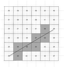
Figure 2: Van Kreveld’s model: (a) Each grid point represents a square cell centered at that point. The elevation angle of all points inside a cell is the same as the elevation angle of the center of the cell (the grid point). (b) To determine if two grid points are visible, we need to consider all cells that intersect the line segment beween the points.

Van Kreveld described a different approach for computing viewsheds on grids that could also be seen as an optimization of R3 [van Kreveld (1996)]. In his model the terrain is seen as a tessellation of square cells, where each cell is centered around a grid point and has the same view angle as the grid point throughout the cell, that is, the cell appears as a horizontal line segment to the viewer (Figure 2). This property allows for the viewshed to be computed in a radial sweep of the terrain in $O(n\lg n)$ time. Because cells have constant view angle, they can be stored in an efficient data structure as the ray rotates around the viewpoint. This data structure supports insertions of cells, deletions of cells, and visibility queries for a point along the ray in $O(\lg n)$ time per operation, and thus the whole viewshed can be computed while rotating the ray in $O(n\lg n)$ time.

The viewshed algorithms mentioned so far assume that the computation fits in memory and are not IO-efficient. I/O-efficient viewshed algorithms have been proposed by Magalhães et al. [Andrade et al. (2011)], Ferreira et al. [Ferreira et al. (2012)] and in our previous work [Haverkort et al. (2008), Fishman et al. (2009), Haverkort et al. (2013)]; we discuss these results below.

Haverkort, Toma and Zhuang [Haverkort et al. (2008)] presented the first IO-efficient viewshed algorithm using Van Kreveld’s model. Using a technique called distribution sweeping they turned Van Kreveld’s algorithm into an algorithm running in $O(n\log n)$ time and $O(\mathsf{sort}(n))$ I/Os, cache-obliviously. The authors also presented practical results showing that their algorithm scales well to large data and outperforms Van Kreveld’s algorithm running in (virtual) memory.

Subsequently, Magalhães et al. [Andrade et al. (2011)] and Ferreira et al. [Ferreira et al. (2012)] described I/O-efficient versions of Franklin’s R2 algorithm. The first algorithm runs in $O(n\log n)$ time and $O(\mathsf{sort}(n))$ I/Os [Andrade et al. (2011)]. As in R2, the idea is to evaluate lines-of-sight only to the points on the perimeter of the grid. To do this I/O-efficiently, the algorithm first copies all grid points from the input file row by row, annotating each point $p$ with the endpoints of the lines of sight whose evaluation requires the elevation of $p$. Next, all annotated points are sorted by line of sight. The algorithm then evaluates each line of sight, determining for each point on a line of sight whether it is visible or not, and writes the results to a file, in order of computation. As a result, the file contains the visibility map, ordered by line of sight. The last step is to sort this file into row-by-row order.

A further improved version of R2 was presented in [Ferreira et al. (2012)]. Here the idea is to partition the grid in blocks and run the (in-memory) version of the R2 algorithm modified so that it bypasses the VMM (virtual memory management) system, and instead it maintains a data structure of “active” blocks that constitute the block footprint of the algorithm. Whenever the line-of-sight intersects a block, that block is brought in main memory. Blocks are evicted using LRU policy. Their algorithm, TiledVS, consists of three passes: convert the grid to Morton order, compute visibility using the R2 algorithm, and convert the output grid from Morton order to row-major order. In practice, this algorithm is much faster than the one in [Andrade et al. (2011)], achieving on the order of 5,000 seconds on SRTM dataset of 7.6 billion points (SRTM1.region06, 28.4GiB using 4 bytes per elevation value) that is, .7$\mu$s per point. Another advantage of TiledVS is that its first step can be viewed as a preprocessing step common to all viewpoints and thus TiledVS computes the viewshed in only two passes over the grid.

The IO-efficient algorithms discussed above differ in how many points they chose to interpolate, how many lines-of-sight they consider, and how they interpolate the terrain. These choices affect both the running time and output of the algorithms. All algorithms described can be considered as approximations of R3 and make some assumptions that they exploit to improve efficiency. TiledVS derives its efficency in part from considering only $O(\sqrt{n})$ LOS’s instead of $O(n)$. Van Kreveld’s approach exploits crucially that cells have constant elevation angle across their azimuth range. Generalizing to linear interpolation is difficult: it would mean that cells have variable elevation angle across their azimuth tange, and one would need a kinetic data structure as active structure to store elevation angles that change in time.

To evaluate viewshed algorithms it is important to consider both efficiency of running time and accuracy of the computed viewshed. While efficiency is easy to compare, comparing accuracy is much harder. The straightforward way to assess accuracy is to compare the computed viewshed with ground truth data. Ideally one would consider a large sample of viewpoints, compute the viewshed from each one in turn, compare it with the real viewshed at that point, and aggregate the differences. Unfortunately, ground truth viewsheds are hard, if not impossible, to obtain.

The algorithms mentioned above assume grid terrains. For an overview of internal-memory algorithms for visibility computations on the second most common format of terrain elevation models, the triangular irregular network or TIN, we refer to  [Cole and Sharir (1989a), de Floriani and Magillo (1994), de Floriani and Magillo (1999)]. Visibility algorithms on TINs use the concept of a horizon or silhouette $\sigma$ of the terrain, which is the upper rim of the terrain, as it appears to a viewer at $v$. More formally, $\sigma_{T}$ is a function from azimuth angles (compass direction) to elevation angles, such that $\sigma_{T}(\alpha)$ is the maximum elevation angle of any point on the intersection of $T$ with the ray that extends from $v$ in direction $\alpha$. On a triangulated terrain, the horizon is equivalent to the upper envelope of the triangle edges of $T$, projected on an infinite vertical cylinder centered on the viewpoint; it has complexity $O(n\cdot\alpha(n))$, where $\alpha$ is the inverse Ackermann function [Cole and Sharir (1989a)]. Horizons have been used to solve various visibility-related problems on triangulated polyhedral terrains. For example, the visibility of all the vertices in a TIN can be computed in $O(n\alpha(n)\lg n)$ time [Cole and Sharir (1989a)]. A central idea in these solutions is that horizons can be merged in time that is linear in their size, and thus allow for efficient divide-and-conquer algorithms.

1.4 Our contributions

This paper describes IO-efficient algorithms for computing viewsheds on massive grid terrains in a couple of different models. Our first two algorithms work in Van Kreveld’s model, and sweep the terrain radially by rotating a ray around the viewpoint while maintaining the terrain profile along the ray. The difference between the two new algorithms is in the preprocessing before the sweep: the first algorithm, which we describe in Section 2, sorts the grid points in concentric bands around the viewpoint; the second algorithm, which we describe in Section 3, sorts the grid points into sectors around the viewpoint. Both algorithms run in $O(n\log n)$ time and $O(\mathsf{sort}(n))$ I/Os.

The third algorithm, io-centrifugal, which we describe in Section 4, uses a complementary approach and sweeps the terrain centrifugally. The algorithm is similar to XDraw: it grows a region around the viewpoint, while maintaining the horizon of the terrain within the region seen so far. To maintain the horizon efficiently, we represent it by a grid model itself: we maintain the maximum elevation angle (the “height”) of the horizon for a discrete set of regularly spaced azimuth angle intervals. The horizontal resolution of the horizon model is chosen to be similar to the horizontal resolution of the original terrain model, so that we maintain elevation angles for $\Theta(\sqrt{n})$ azimuth angle intervals. This allows a significant speed-up as compared to algorithms that process events at $\Theta(n)$ different azimuth angles, or work with horizons of linear complexity. Also, we note that this gives the algorithm the potential for higher accuracy than XDraw, which represents the horizon up to a given layer by only as many grid points as there are in that layer—which can be quite inaccurate close to the viewpoint. Another difference with XDraw is that our algorithm does not proceed layer by layer, but instead grows the region in a recursive, more I/O-efficient way; this results in a significant speed-up in practice. The centrifugal sweep algorithm runs in $O(n)$ time and $O(\mathsf{scan}(n))$ I/Os cache-obliviously, and is our fastest algorithm.

Our last two algorithms constitute an improved, IO-efficient version of Franklin’s R3 algorithm. We distinguish between two models (Figure 7), which we describe in Section 5: In the gridlines model we view the points in the input grid as connected by horizontal and vertical lines, and visibility is determined by evaluating the intersections of the line-of-sight with the grid lines using linear interpolation; this is the model underlying R3.

We also consider a slightly different model, the layers model, in which we view the points in the input grid to be connected in concentric layers around the viewpoint and visibility is determined by evaluating the intersections of the line-of-sight with these layers using linear interpolation. The layers model considers only a subset of the intersections considered by the gridlines model and therefore the viewshed generated will be larger (more optimistic) than the one generated with the gridlines model. Preliminary results ([Fishman et al. (2009)]) show that these differences are practically insignificant. The layers model is faster in practice, while having practically the same accuracy as the gridlines model.

We describe our last two algorithms, vis-iter and vis-dac, in Section 5. They are based on computing and merging horizons in an iterative or divide-and-conquer approach, respectively. Horizon-based algorithms for visibility problems have been described by de Floriani and Magillo [de Floriani and Magillo (1994)]. On a triangulated terrain $T$, the horizon is equivalent to the upper envelope of the triangle edges of $T$ as projected on a view screen, and has complexity $H(n)=O(n\cdot\alpha(n))$, where $n$ is the number of vertices in the TIN and $\alpha()$ is the inverse of the Ackerman function [Cole and Sharir (1989b)]. In Section  5.1 we show that we can prove a better bound for our setting: that is, we prove that the upper envelope of a set $S$ of line segments in the plane such that the widths of the segments do not differ in length by more than a factor $d$ has complexity $O(dn)$. From here we show that the horizon on a grid of $n$ points with linear interpolation has complexity $O(n)$ in the worst case.

In Section 6 we describe an experimental analysis and comparison of our algorithms on datasets up to 28 GB. All algorithms are scalable to volumes of data that are more than 50 times larger than the main memory. Our main finding is that, in practice, horizons are significantly smaller than their theoretical upper bound, which makes horizon-based algorithms unexpectedly fast. Our last two algorithms, which compute the most accurate viewshed, turn out to be very fast in practice, although their worst-case bound is inferior. We conclude in Section 7.

2 I/O-Efficient radial sweep

This section describes our first approach to computing a viewshed. It is loosely based on Van Kreveld’s radial sweep algorithm, which we present below.

The model. We consider that the terrain is represented by a set of $n$ points whose projections on $D$ form a regular grid with inter-point distance 1. Furthermore, we assume that each grid point $q=(q_{x},q_{y},q_{z})$ represents a square “cell” $D(q)$ on $D$ of size $1\times 1$, centered on $(q_{x},q_{y})$. For any given viewpoint $v$, we treat the terrain above $D(q)$ as if each point of $D(q)$ has elevation angle $\textrm{ElevAngle}(q)$. This is the interpolation method used by Van Kreveld [van Kreveld (1996)]. Determining whether a point $p$ is visible from viewpoint $v$ comes down to deciding whether there is any other grid point $q$ such that the square cell $D(q)$ intersects the line segment from $(v_{x},v_{y})$ to $(p_{x},p_{y})$ and $\textrm{ElevAngle}(q)\geq\textrm{ElevAngle}(p)$; see Figure 2.

2.1 Van Kreveld’s radial sweep algorithm

The basic idea of Van Kreveld’s algorithm [van Kreveld (1996)] is to rotate a half-line (ray) around the viewpoint $v$ and compute the visibility of each grid point in the terrain when the sweep line passes over it (see Figure 3). For this we maintain a data structure (the active structure) that, at any time in the process, stores the elevation angles for the cells currently intersected by the sweep line (the active cells). Three types of events happen during the sweep:

• enter events: When a cell starts being intersected by the sweep line, it is inserted in the active structure;

• center events: When a the sweep line passes over the grid point $q$ at the center of a cell, the active structure is queried to find out if $q$ is visible.

• exit events: When a cell stops being intersected by the sweep line, it is deleted from the active structure;

Thus, each cell in the grid has three associated events. Van Kreveld [van Kreveld (1996)] uses a balanced binary search tree for the active structure, in which the active cells are stored in order of increasing distance from the viewpoint. Because the cells are convex, this is always the same as ordering the active cells in order of increasing distance from the viewpoint to pothe grid points corresponding to the cells. With each cell we store its elevation angle. In addition, each node in the tree is augmented with the highest elevation angle in the subtree rooted at that node. A query if a point $q$ is visible is answered by checking if the active structure contains any cell that lies closer to the viewpoint than $q$ and has elevation angle at least $\mathrm{ElevAngle}(q)$: if yes, then $q$ is not visible, otherwise it is. Such a query can be answered in $O(\log n)$ time. To run the complete algorithm, we first generate and sort the $3n$ events by their azimuth angles (the sweep line directions at which they happen). Then we process the events in order of increasing azimuth angle. The whole algorithm runs in $O(n\log n)$ time.

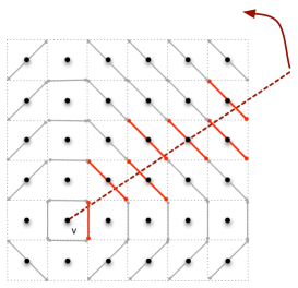
Figure 3: Van Kreveld algorithm. Cells will be present in the active structure as long as the sweep ray intersects the indicated diagonal.

In our previous work we adapted Van Kreveld’s algorithm to make it I/O-efficient [Haverkort et al. (2008)]. The first step was still to generate and sort the events. For each event we stored its location in the plane and its elevation angle. Using four bytes per coordinate, this resulted in an event stream of $36n$ bytes. For large $n$, this is a significant bottleneck.

2.2 A new I/O-efficient radial sweep algorithm

The main idea of our new radial sweep algorithm is therefore to avoid generating and sorting a fully specified event stream. The purpose of the event stream was to supply the azimuth angle and the elevation angle of the events in order. Note, however, that the azimuth angle of the events only depends on how the sweep progresses over the grid, but not on the elevation values stored in the input file. Only the elevation angles have to be derived from the input file.

Our ideas for making the sweep I/O-efficient are now the following. We can compute the azimuth angles of the events on the fly, without accessing the input file, instead of computing all events in advance. Only when processing an enter event corresponding to a grid point $q$, the elevation of $q$ needs to be retrieved in order to insert $\langle\mathrm{Dist}(q),\mathrm{ElevAngle}(q)\rangle$ into the active structure—for center events the elevation angle can then be found in the active structure and for exit events the elevation angle is not needed. To allow efficient retrieval of elevations for enter events, we pre-sort the elevation grid into lists of elevation values, stored in the order of the enter events that require them. Thus we can retrieve all elevation values in $O(\mathsf{scan}(n))$ I/Os during the sweep. Sorting the complete elevation grid into a single list would be relatively expensive (it would require several sorting passes); we avoid that by dividing the grid into concentric bands around the viewpoint, making one list of elevation values for each band. As long as the number of bands in small enough so that we can keep a read buffer of size $\Theta(B)$ for each band in memory during the sweep, we will still be able to retrieve all elevation values during the sweep in $\Theta(\mathsf{scan}(n))$ I/Os.

Notation. For ease of description, assume that the viewpoint $v$ is in the center of the grid at coordinates $(0,0,0)$ and the grid has size $(2m+1)\times(2m+1)$, where $m=(\sqrt{n}-1)/2$. The elevations of the grid points are given in a two-dimensional matrix $Z$ that is ordered row by row, with rows numbered from $-m$ to $m$ from north to south and columns numbered from $-m$ to $m$ from west to east. By $p(i,j)$ we denote the grid point $q=(q_{x},q_{y},q_{z})$ in row $i$ and column $j$ with coordinates $q_{x}=j$, $q_{y}=-i$ and $q_{z}=Z_{ij}$; by cell $(i,j)$ we denote the square $D(p(i,j))$. Let $\textsc{enter}(i,j)$ denote the azimuth angle of the enter event of cell $(i,j)$.

Description of the algorithm. We now describe our algorithm in detail. Let layer $l$ of the grid denote the set of grid points whose $L_{\infty}$-distance from the viewpoint, measured in the horizontal plane, is $l$. We divide the grid in concentric bands of width $w$ around the viewpoint. Band $k$ (denoted $B_{k}$), with $k>0$, contains all grid points of layers $(k-1)w+1$ up to $kw$, inclusive; so $p(i,j)$ would be found in band $\lceil\max(|i|,|j|)/w\rceil$ (see Figure 4). We choose $w=\Theta(\sqrt{M})$; more precisely, $w$ is the largest power of two such that the elevation and visibility values of a square tile of $(w+1)\cdot(w+1)$ points fit in one third of the memory.

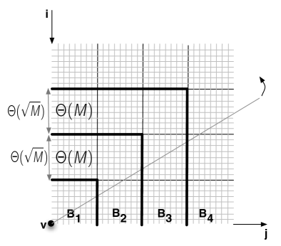
Figure 4: A layered radial sweep.

Our algorithm proceeds in three phases. The first phase is to generate, for each band $B_{k}$, a list $E_{k}$ containing the elevations of all points $p(i,j)$ in the band, ordered by increasing $\textsc{enter}(i,j)$ values (recall that $\textsc{enter}(i,j)$ denotes the azimuth angle of the enter event of the cell $(i,j)$). Points $p(i,j)$ with the same $\textsc{enter}(i,j)$ value are ordered secondarily by increasing distance $\mathrm{Dist}(i,j)$ from the viewpoint. The algorithm that builds the lists $E_{k}$ is given below. The basic idea is to read the grid points from the elevation grid going in counter-clockwise order around the viewpoint. This is achieved by maintaining a priority queue with points just in front of the sweep line; the priority queue is organised by the azimuth angles of the enter events corresponding to the points to be read. The queue is initialised with all points of $B_{k}$ that lie straight right of the viewpoint (Note: such a point $(0,j)$ will have its $\textsc{enter}(0,j)$ given by the south-west corner of its cell at $(1/2,j-1/2)$ which corresponds to an angle in the fourth quadrant $(3\pi/2,2\pi)$; we subtract $2\pi$ to bring it to $(-\pi/2,0)$; this guarantees that points straight right of the viewpoint are first in radial order). Then we extract points from the queue one by one in order of increasing $\textsc{enter}(i,j)$; when we extract a point, we read its elevation from the elevation grid, write the elevation value to $E_{k}$, and insert the next point from the same layer in the priority queue (this is the point above, to the left, below, or to the right, depending on which octant the current point is in). In this way, from neighbor to neighbor, all points are eventually reached. Below we describe the algorithm only for the first quadrant (Figure 4); the others are handled similarly.

Algorithm BuildBands:
for $k\leftarrow 1$ to $\lceil m/w\rceil$
do initialise empty list $E_{k}$ and priority queue $Q$
do for $j\leftarrow(k-1)\cdot w+1$ to $k\cdot w$
do do insert $\langle\textsc{enter}(0,j)-2\pi,0,j\rangle$ into $Q$
do while $E_{k}$ is not complete
do do $\langle\alpha,i,j\rangle\leftarrow Q$.deleteMin()
do do read $Z_{ij}$ from the grid and write it to $E_{k}$
do do if $-i<j$ (next cell is north)
do do then insert $\langle\textsc{enter}(i-1,j),i-1,j\rangle$ into $Q$
do do else (next cell is west)
do do then insert $\langle\textsc{enter}(i,j-1),i,j-1\rangle$ into $Q$
do clear $Q$

After constructing the lists $E_{k}$, the second phase of the algorithm starts: computing which points are visible. To do this we perform a radial sweep of all events in azimuth order. Again, we generate the events on the fly with the help of a priority queue, using only the horizontal location of the grid points. We use a priority queue to hold events in front of the sweep line, and an active structure to store the cells that currently intersect the sweep line, sorted by increasing distance from the viewpoint (as in Van Kreveld’s algorithm). The algorithm starts by inserting all enter events of the points straight to the right of the viewpoint into the priority queue. When the next event in the priority queue is an enter event for cell $(i,j)$, the algorithm inserts the corresponding center and exit events in the queue, as well as the enter event of the next cell in the same layer. In addition, it reads the elevation $Z_{ij}$ of $p(i,j)$ from the list of elevation values $E_{k}$ of the band $B_{k}$ that contains $p(i,j)$, and it inserts the cell $(i,j)$ in the active structure with key $\textrm{Dist}(i,j)$. When the next event in the priority queue is a center event for cell $(i,j)$, the algorithm queries the active structure for the visibility of the point with key $\textrm{Dist}(i,j)$. When the next event in the priority queue is an exit event for cell $(i,j)$, the algorithm deletes the element with key $\textrm{Dist}(i,j)$ from the active structure.

Algorithm ComputeVisibility:
Initialise empty active structure $A$ and priority queue $Q$
for $j\leftarrow 1$ to $m$
do insert $\langle\textsc{enter}(0,j)-2\pi,\textsc{enter},0,j\rangle$ into $Q$
for $k\leftarrow 1$ to $\lceil m/w\rceil$
do set read pointer of $E_{k}$ at the beginning
do initialise empty list $V_{k}$
while not all visibility values have been computed
do $\langle\alpha,\mathit{type},i,j\rangle\leftarrow Q$.deleteMin()
do if $\mathit{type}=\textsc{enter}$
do then insert $\langle\textsc{center}(i,j),\textsc{center},i,j\rangle$ in $Q$
do then insert $\langle\textsc{exit}(i,j),\textsc{exit},i,j\rangle$ into $Q$
do then if $|i|<j$ or $i=j>0$  (next cell is north)
do then then insert $\langle\textsc{enter}(i-1,j),\textsc{enter},i-1,j\rangle$ in $Q$
do then [… similar for west, south, and east …]
do then compute band number $k\leftarrow\lceil\max(|i|,|j|)/w\rceil$
do then $z\leftarrow$ the next unread value from $E_{k}$
do then $\beta\leftarrow\arctan(z/\mathrm{Dist}(i,j))$  ($=\mathrm{ElevAngle}(p(i,j))$)
do then insert $\langle\mathrm{Dist}(i,j),\beta\rangle$ into $A$
do else if $\mathit{type}=\textsc{center}$
do then compute band number $k\leftarrow\lceil\max(|i|,|j|)/w\rceil$
do then query $A$ if element with key $\mathrm{Dist}(i,j)$ is visible;
do then if yes, write 1 to $V_{k}$, otherwise write 0 to $V_{k}$
do else ($\mathit{type}=\textsc{exit}$)
do then delete element with key $\mathrm{Dist}(i,j)$ from $A$

The crux of the ComputeVisibility algorithm above is the following: when it needs to read $Z_{ij}$, it simply takes the next unread value from its band $E_{k}$. This is correct, because within each band $B_{k}$, the above algorithm requires the $Z_{ij}$ values in the order of the corresponding enter events, and this is exactly the order in which these values were put in $E_{k}$ by algorithm BuildBands. The output of the second phase is a number of lists $V_{k}$ with visibility values: one list for each band, in order of the azimuth angle of the grid points.

The third phase of the algorithm sorts the lists $V_{k}$ into one visibility map. To do so we run an algorithm that is more or less the reverse of algorithm BuildBands: we only need to swap the roles of reading and writing, and use azimuth values for center events instead of enter events.

Efficiency analysis. We will now argue that the above algorithm computes a visibility map in $O(n\log n)$ time and $O(\mathsf{scan}(n))$ I/Os under the assumption that the input grid is square, and we have $M\geq c_{1}\sqrt{n}$ and $M\geq c_{2}B^{2}$ for sufficiently large constants $c_{1}$ and $c_{2}$.

We start with the first phase: BuildBands. Consider the part of band $B_{1}$ which lies in the first quadrant. This part consists of all points $p(i,j)$ such that $0\leq-i\leq w$ and $0\leq j\leq w$ (except the viewpoint itself). It is a tile of size $(w+1)\cdot(w+1)$, which fits in one third of the main memory by definition of $w$. As the algorithm iterates through the points of $B_{1}$, it accesses their elevations, loading blocks from disk, until eventually the entire tile is in main memory, after which there are no subsequent I/O-operations on the input grid. The number of I/Os to access the tile is $O(w+w^{2}/B)=O(\sqrt{M}+M^{2}/B)$. By the assumption that $M=\Omega(B^{2})$, this is $O(M^{2}/B)=O(|B_{1}|/B)$, where $|B_{1}|$ denotes the number of grid points in $B_{1}$. In fact any band $B_{k}$ with $k\geq 1$ can be subdivided into $8k-4$ tiles of size at most $(w+1)\cdot(w+1)$, such that for any band, the sweep line will intersect at most two such tiles at any time (see Figure 4). Since a tile fits in at most one third of the memory, two tiles fit in memory together. Therefore the algorithm can process each band by reading tiles one by one, without ever reading the same tile twice. Thus each band $B_{k}$ is read in $O(\mathsf{scan}(|B_{k}|))$ I/Os, and algorithm BuildBands needs $O(\mathsf{scan}(n))$ I/Os in total to read the input. The output lists $E_{k}$ are written sequentially, taking $O(\mathsf{scan}(n))$ I/Os as well. It remains to discuss the operation of the priority queue. Note that at any time the priority queue stores one cell from each layer, and therefore it has size $m<\frac{1}{2}\sqrt{n}$; by assumption this is at most $\frac{1}{2}M/c_{1}$. Hence, for a sufficiently large value of $c_{1}$, the priority queue fits in memory together with the two tiles from the input file mentioned above (which each take at most one third of the memory). Thus the operation of the priority queue takes no I/O, but it will take $O(\log n)$ CPU-time per operation, and thus, $O(n\log n)$ time in total.

The second phase, ComputeVisibility, reads and writes each list $E_{k}$ and $V_{k}$ in a strictly sequential manner. There are $O(m/w)=O(\sqrt{n/M})$ bands. Under the assumption $M\geq c_{1}\sqrt{n}$ and $M\geq c_{2}B^{2}$, this is only $O(\sqrt{n/M})=O(\sqrt{n}/B)=O(M/B)$. This implies that, when $c_{1}$ and $c_{2}$ are sufficiently high constants, one block from each list $E_{k}$ or $V_{k}$ can reside in memory as a read or write buffer during the sweeping. Thus all lists $E_{k}$ and $V_{k}$ can be read and written in parallel in $O(\mathsf{scan}(n))$ I/Os in total. The priority queue and the active structure have size $O(\sqrt{n})$ and therefore fit in memory by the arguments given above, so the second phase needs $O(n\log n)$ time and $O(\mathsf{scan}(n))$ I/Os in total.

The third phase, sorting the output lists into a visibility grid, also takes $O(n\log n)$ time and $O(\mathsf{scan}(n))$ I/Os: the analysis is the same as for the first phase. Note that in practice, the number of visible points is often very small compared to the size of the grid. In that case it may be better to change the algorithm ComputeVisibility as follows: instead of writing the visibility values of all grid points to separate lists for each band and sorting these into a grid, we record only the visible grid points with their grid coordinates, write them to a single list $V$, sort this list, and produce a visibility map from the sorted output.

2.3 An algorithm for very large inputs

The above algorithm computes a visibility map in $\Theta(\mathsf{scan}(n))$ I/Os under the assumption that $M\geq c_{1}\sqrt{n}$, and $M\geq c_{2}B^{2}$ for sufficiently large constants $c_{1}$ and $c_{2}$. Note that $\mathsf{sort}(n)=\Theta(\mathsf{scan}(n))$ under these assumptions. The idea of a layered radial sweep can be extended to a recursive algorithm that runs in $O(\mathsf{sort}(n))$ I/Os for any $n$, without both these assumptions.

The idea is the following: we divide the problem into $\Theta(M/B)$ bands, scan the input to distribute the grid points into separate lists for each band, then compute visibility recursively in each band, and merge the results. More precisely, for each band we will compute a list of “locally” visible points and a “local” horizon: these are the points and the horizon that would be visible in absence of the terrain between the viewpoint and the band. The list of visible points is stored in azimuth order around the viewpoint. The horizon is a step function whose complexity is linear in the number of points of the terrain; it is also stored as a list of points in azimuth order around the viewpoint.

Now we can merge two adjacent bands as follows. Let $V_{1}$ and $H_{1}$ be the list of visible points and the horizon of the inner band, and let $V_{2}$ and $H_{2}$ be the list of visible points and the horizon of the outer band. The merge proceeds as follows. We scan these four lists in parallel, in azimuth order, and output two lists in azimuth order. First, a list of visible points containing all points of $V_{1}$, and all points $V_{2}$ that are visible above $H_{1}$. Second, the merged horizon: the upper envelope of $H_{1}$ and $H_{2}$. This correctly computes visibility because a point is visible if and only if is visible in its band, and is not occluded by any of the bands that are closer to $v$.

The idea of the merge step can be extended to merge $M/B$ bands, resulting in an algorithm that runs in $O(\mathsf{sort}(n))$ I/Os. To see why, observe that there are $\Theta(M/B)$ levels of recursion, and the base-case runs in linear time. Each band and its horizon have size $O(n/(M/B))$. The merging can be performed in linear time because it involves scanning of $\Theta(M/B)$ lists of size $\Theta(n/(M/B))$; a block from each list fits in memory and the total size of all lists is $\Theta(n)$. It remains to show that a horizon can be computed in linear time in a base-case band of width $\Theta(\sqrt{M})$. To see this, we note that a band consists of tiles of size $\sqrt{M}\cdot\sqrt{M}$, and the horizon can be computed tile by tile. The details are similar to ones already discussed, and we omit them.

Overall, we get a divide-and-conquer algorithm that can compute visibility in $\Theta(\mathsf{sort}(n))$ I/Os for any $n$, assuming $M\geq c_{2}B^{2}$. Because another algorithm with a theoretical I/O-efficiency of $O(\mathsf{sort}(n))$ was already known from our previous work [Haverkort et al. (2008)], this “new” divide-and-conquer algorithm is not particularly interesting. In practice such a recursive algorithm would probably never be needed: it would only be useful when $n$ would be at least as big as $(M/c_{1})^{2}$.

3 A radial sweep in sectors

This section describes our second algorithm for computing the visibility map of a point $v$. It does not achieve better asymptotic bounds on running time and I/Os than the algorithm from the previous section, but, as we will see in Section 6, it is faster. Like the algorithm from Section 2, our second algorithm sweeps the terrain radially around the viewpoint. As before, the azimuth angles of the events are computed on the fly using a priority queue. Elevation values of grid points are only needed when their enter events are processed. To make access to elevation values efficient, we first divide the elevation grid into sectors of $\Theta(M)$ grid points each—this is the main difference with the algorithm from the previous section, which divided the elevation grid into concentric bands.

The algorithm proceeds in three phases. First, for any pair of azimuth angles $\alpha,\beta$, let $S(\alpha,\beta)$ be the set of grid points whose corresponding enter events have azimuth angle at least $\alpha$ and less than $\beta$. The first phase of our algorithm starts by computing a set of azimuth angles $\alpha_{0}<...<\alpha_{s}$, where $\alpha_{0}=0$ and $\alpha_{s}=2\pi$, such that for any $1\leq k\leq s$ we have that the coordinates and elevation values of $S(\alpha_{k-1},\alpha_{k})$ fit in one third of the main memory. Note that this can be done without accessing the elevation grid: the algorithm only needs to know the size of the grid and the location of the viewpoint in order to be able to divide the full grid into memory-size sectors. We then scan the elevation grid and distribute the grid points based on their enter azimuth angle into lists: one list $E_{k}$ for each sector $S(\alpha_{k-1},\alpha_{k})$. (Cells straight right of the viewpoint need to be entered at the beginning of the sweep and are additionally put in $E_{1}$).

In the second phase we do the radial sweep as before, sector by sector, with two modifications: (i) whenever we enter a new sector $S(\alpha_{k-1},\alpha_{k})$, we load the complete list $E_{k}$ into memory and sort it by the azimuth angle of the enter events; (ii) we do not keep a list of visibility values per sector, but instead we write the row and column coordinates of the points that are found to be visible to a single list $L$.

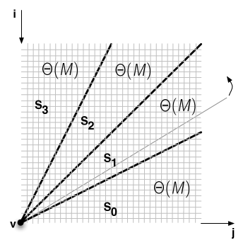
Figure 5: A radial sweep in sectors.

Finally, in the third phase we sort $L$ and scan it to produce a visibility map of the full grid. Thus the full algorithm is as follows:

Algorithm SectoredSweep:
First phase—distribution:
Compute sector boundaries $\alpha_{0},...,\alpha_{s}$ analytically such that each sector $S(\alpha_{k-1},\alpha_{k})$ fits in one third of the memory.
for $k\leftarrow 0$ to $s$
do initialise empty list $E_{k}$
for all points $p(i,j)$ in row-by-row order (except $v$)
do compute $k$ s.t. $\alpha_{k-1}\leq\textsc{enter}(i,j)<\alpha_{k}$
do read $Z_{ij}$ and write $\langle i,j,Z_{ij}\rangle$ to $E_{k}$
for all points $p(i,j)$ from $v$ (excl.) straight to the right
do read $Z_{ij}$ and write $\langle i,j,Z_{ij}\rangle$ to $E_{0}$
Second phase—sweep:
initialise empty active structure $A$ and priority queue $Q$
initialise empty output list $L$
for $j\leftarrow 1$ to $m$
do insert $\langle\textsc{enter}(0,j)-2\pi,\textsc{enter},0,j\rangle$ into $Q$
$k\leftarrow 1$; load $E_{1}$ in memory and sort it by $\textsc{enter}(i,j)$
while not all visibility values have been computed
do $\langle\alpha,\mathit{type},i,j\rangle\leftarrow Q$.deleteMin()
do if $\mathit{type}=\textsc{enter}$
do then if $E_{k}$ contains no more unread elements
do then then delete $E_{k}$; $k\leftarrow k+1$; load $E_{k}$ in memory
do then then sort $E_{k}$ and set read pointer at beginning
do then $z\leftarrow$ read the next unread value from $E_{k}$  (=$Z_{ij}$)
do then $\beta\leftarrow\arctan(z/\mathrm{Dist}(i,j))$  ($=\mathrm{ElevAngle}(p(i,j))$)
do then insert $\langle\mathrm{Dist}(i,j),\beta\rangle$ into $A$
do then insert $\langle\textsc{center}(i,j),\textsc{center},i,j\rangle$ in $Q$
do then insert $\langle\textsc{exit}(i,j),\textsc{exit},i,j\rangle$ into $Q$
do then if $|i|<j$ or $i=j>0$  (next cell is north)
do then then insert $\langle\textsc{enter}(i-1,j),\textsc{enter},i-1,j\rangle$ in $Q$
do then [… similar for west, south, and east …]
do else if $\mathit{type}=\textsc{center}$
do then query $A$ if element with key $\mathrm{Dist}(i,j)$ is visible;
do then if yes, write $\langle i,j\rangle$ to $L$
do else ($\mathit{type}=\textsc{exit}$)
do then delete element with key $\mathrm{Dist}(i,j)$ from $A$
Third phase—produce visibility map:
Sort $L$ lexicographically by row, column
Set read pointer of $L$ at the beginning
for all points $p(i,j)$ in row-by-row order
do if next element of $L$ is $(i,j)$
do then $V_{ij}\leftarrow 1$; advance read pointer of $L$
do else $V_{ij}\leftarrow 0$

Efficiency analysis. We will now briefly argue that the above algorithm computes a visibility map of the first quadrant in $O(n\log n)$ time and $O(\mathsf{scan}(n)+\mathsf{sort}(t))$ I/Os, where $t$ is the number of visible grid points, under the assumption that the input grid is square and $M^{2}/B\geq cn$ for a sufficiently large constant $c$.

The first phase of the algorithm reads the elevation grid once and writes elevation values to $O(n/M)=O(M/B)$ sector lists. Therefore we can keep, for each sector, one block of size $\Theta(B)$ in memory as a write buffer, and thus the first phase produces the sector lists in $O(\mathsf{scan}(n))$ I/Os. The running time of the first phase is $\Theta(n)$.

During the second phase, we read the sector lists one by one, in $O(\mathsf{scan}(n))$ I/Os in total. The priority queue and the active structure can be maintained in memory by the arguments given in the previous section. Creating and sorting $L$ takes $O(\mathsf{sort}(t))$ I/Os, after which it is scanned to produce a visibility map.

Thus the algorithm runs in $O(n\log n)$ time and $O(\mathsf{scan}(n)+\mathsf{sort}(t))$ I/Os.

An algorithm for very large inputs. When the assumption $M^{2}/B\geq cn$ does not hold, a radial sweep based on distribution into sectors is still possible: one can use the recursive distribution sweep algorithm from our previous work [Haverkort et al. (2008)] and apply the ideas described above to reduce the size of the event stream. The result is an algorithm that runs in $O(n\log n)$ time and $O(\mathsf{sort}(n))$ I/Os. We sketch the main ideas below.

First we note that, for large $n$, the “diagonal” of the grid is larger than $M$ and does not fit in a sector. The splitter values for sectors can still be computed without any I/O because they depend solely on the position $(i,j)$ of the points wrt $v$, and not on their elevation. For example, one could do a pass through the points in $\textsc{enter}(i,j)$ order using an I/O-efficient priority queue, in the same way as during the sweep, but without accessing the elevation. Using a counter we can keep track of the number of points processed, and output every $\Theta(M)$-th one as a splitter.

Given the splitters, we can proceed recursively: first distribute the grid into $\Theta(M/B)$ sectors, and then distribute each sector recursively until each sector has size $\Theta(M)$. This takes $\Theta(\log_{M/B}n)$ passes over the grid. Thus, distribution into $\Theta(M)$-sized sectors can be performed in $\Theta(\mathsf{sort}(n))$ I/Os. If $n>M^{2}$, the active structure does not fit in memory and the sweep of the sectors with a common active structure does not work, even though each sector is $\Theta(M)$. We need to refine the distribution to process carefully long cells that span more than one sector, so that we can process each sector individually. This can be done I/O-efficiently in $\Theta(\mathsf{sort}(n))$ I/Os and we refer to our previous algorithm for details [Haverkort et al. (2008)].

4 A centrifugal sweep algorithm

In this section we describe our third algorithm for computing the visibiliy map. It uses a complementary approach to the radial sweep in the previous sections and sweeps the terrain centrifugally, by growing a region $R$ around the viewpoint. This region is kept star-shaped around $v$: for any point $u$ inside $R$, the line segment from $(u_{x},u_{y})$ to $(v_{x},v_{y})$ lies entirely inside $R$. The idea is to grow $R$ point by point until it covers the complete grid, while maintaining the horizon $\sigma_{R}$ of $R$. Recall that the horizon $\sigma_{R}$ is a function from azimuth angles to elevation angles, such that $\sigma_{R}(\alpha)$ is the maximum elevation angle of any point on the intersection of $R$ with the ray that extends from $v$ in direction $\alpha$.

Whenever a new point $u$ is added to $R$, we decide whether it is visible. The star shape of $R$ guarantees that all points along the line of sight from $v$ to $u$ have already been added, so we can in fact decide whether $u$ is visible by determining whether $u$ is visible above the horizon of $R$ just before adding $u$ (see Figure 6). The key to a good performance is to have a way of growing $R$ that results in an efficient disk access pattern, and to have an efficient way of maintaining the horizon structure. Below we explain how to do this, given an elevation grid with a fixed number of bytes per grid point.

For ease of description, we remind the reader our notation: We assume that the viewpoint $v$ is in the center of the grid at coordinates $(0,0,0)$ and the grid has size $(2m+1)\times(2m+1)$, where $m=(\sqrt{n}-1)/2$. The elevations of the grid points are given in a two-dimensional array $Z$ that is ordered row by row, with rows numbered from $-m$ to $m$ from north to south and columns numbered from $-m$ to $m$ from west to east. By $p(i,j)$ we denote the grid point $q=(q_{x},q_{y},q_{z})$ in row $i$ and column $j$ with coordinates $q_{x}=j$, $q_{y}=-i$ and $q_{z}=Z_{ij}$; by cell $(i,j)$ we denote the square $D(p(i,j))$.

To maintain the horizon efficiently, we represent it by a grid model itself: more precisely, it is maintained in an array $S$ of $32m$ slots, where slot $i$ stores the highest elevation angle in $R$ that occurs within the azimuth angle range from $i\cdot 2\pi/32m$ to $(i+1)\cdot 2\pi/32m$.

For growing the region $R$ the idea is to do so cache-obliviously using a recursive algorithm. Initially we call this algorithm with the smallest square that contains the full grid and whose width is a power of two. When called on a square of size larger than one, it makes recursive calls on each of the four quadrants of the square, in order of increasing distance of the quadrants from $v$. For a square tile with upper left corner $(i,j)$ and width $s$, this distance $\mathrm{TileDist}(i,j,s)$ is the distance from $v$ to the closest point of the tile. This is determined as follows. Let $v_{i},v_{j}$ be the row and column of the viewpoint.

• when $i\leq v_{i}<i+s$ and $j\leq v_{j}+s$, then the tile contains $v$, and $\mathrm{TileDist}(i,j,s)=0$;

• otherwise, when $i\leq v_{i}<i+s$, the tile intersects the row that contains $v$, and $\mathrm{TileDist}(i,j,s)=\min(|i-v_{i}|,|i+s-1-v_{i}|)$;

• otherwise, when $j\leq v_{j}<j+s$, the tile intersects the column that contains $v$, and $\mathrm{TileDist}(i,j,s)=\min(|j-v_{j}|,|j+s-1-v_{j}|)$;

• otherwise, $\mathrm{TileDist}(i,j,s)=\min(|i-v_{i}|+|j-v_{j}|,|i-v_{i}|+|j+s-1-v_{j}|,|i+s-1-v_{i}|+|j-v_{j}|,|i+s-1-v_{i}|+|j+s-1-v_{j}|)$.

When called on a square of size 1, that is, a square that contains only a single grid point $p(i,j)$, we proceed as follows. We retrieve the elevation $Z_{ij}$ of $p(i,j)$ from the input file and compute its azimuth angle $\mathrm{AzimAngle}(p(i,j))$ and its elevation angle. $\mathrm{ElevAngle}(p(i,j))$. Then we check if $p(i,j)$ is visible: this is the case if and only if $p(i,j)$ appears higher above the horizon than the current horizon in the direction of $p(i,j)$; that is, if and only if $\mathrm{ElevAngle}(p(i,j))>S[\lfloor\mathrm{AzimAngle}(p(i,j))/2\pi\cdot 32m\rfloor]$. The visibility of $p(i,j)$ is recorded in the output grid $V$. Next we update the horizon to reflect the inclusion of $p(i,j)$ in $R$. To this end we check all slots in the horizon array whose azimuth angle range intersects the azimuth angle range of cell $(i,j)$; let ${\cal A}(p(i,j))$ denote this set of slots. For each slot of ${\cal A}(p(i,j))$ that currently stores an elevation angle lower than $\mathrm{ElevAngle}(p(i,j))$, we raise the elevation angle to $\mathrm{ElevAngle}(p(i,j))$. We thus have the following algorithm:

Algorithm CentrifugalSweep:
create horizon array $S[0..32m-1]$
for $k\leftarrow 0$ to $32m-1$ do $S[k]\leftarrow-\infty$
$s\leftarrow$ smallest power of two $\geq 2m+1$
$\textsc{SweepRecursively}(\mathit{-m,-m,s})$

Algorithm $\textsc{SweepRecursively}(i,j,s)$:
(Recursively computes visibility for the tile with upper left cell $(i,j)$ and width $s$)
if $s=1$
then $\alpha\leftarrow\mathrm{AzimAngle}(p(i,j))$
then $\beta\leftarrow\arctan(Z_{ij}/\mathrm{Dist}(i,j))$ ($=\mathrm{ElevAngle}(p(i,j))$)
then if $\beta>S[\lfloor\alpha/2\pi\cdot 32m\rfloor]$ then $V_{ij}\leftarrow 1$ else $V_{ij}\leftarrow 0$
then $\alpha^{-}\leftarrow$ smallest azimuth of any corner of cell $(i,j)$
then $\alpha^{+}\leftarrow$ largest azimuth of any corner of cell $(i,j)$
then for $k\leftarrow\lfloor\alpha^{-}/2\pi\cdot 32m\rfloor$ to $\lceil\alpha^{+}/2\pi\cdot 32m\rceil-1$
then do $S[k]\leftarrow\max(S[k],\beta)$
else Let $Q$ be the four subquadrants:
then $s\leftarrow s/2$
then $Q\leftarrow\{\langle i,j,s\rangle,\langle i+s,j,s\rangle,\langle i,j+s,s\rangle,\langle i+s,j+s,s\rangle\}$
then sort the elements $\langle i,j,s\rangle$ of $Q$ by incr. $\mathrm{TileDist}(i,j,s)$
then for $\langle i,j,s\rangle\in Q$
then do $\textsc{SweepRecursively}(i,j,s)$

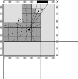
Figure 6: $R$ (dark shade) is a star-shaped region of the terrain (light shade) around $v$. The horizon of $R$ is maintained in array $S$. When $u$ is added to $R$, the elevation angles in the black slots of $S$ are updated.

4.1 Accuracy of the centrifugal sweep

Note that when the algorithm updates the horizon array, the elevation angle of $p(i,j)$ may be used to raise the elevation angles of a set of horizon array slots ${\cal A}(p(i,j))$, of which the total azimuth range may be slightly larger than that of the cell corresponding to $p(i,j)$—this is due to the rounding of the azimuth angles $\alpha^{-}$ and $\alpha^{+}$ in the algorithm. However, this is not a problem: The azimuth angles of grid points that lie next to each other (as seen from the viewpoint) differ by at least roughly $1/m$. The size of the horizon array is chosen such that its horizontal resolution is more than four times bigger: it divides the full range of azimuth angles from $0$ to $2\pi$ over $32m$ slots, each of which covers an azimuth angle range of $2\pi/32m<1/4m$. Therefore, if the resolution of the horizon array would be insufficient, then surely the resolution of the original elevation grid would not be sufficient.

4.2 Efficiency of the centrifugal sweep

The number of recursive calls made by the region-growing algorithm is $O(n)$. The only part of any recursive call that takes more than constant time is the updating of the horizon. We analyse this layer by layer, where this time layer $l$ is defined as the cells $(i,j)$ such that $|i|+|j|=l$. There are $O(\sqrt{n})$ layers, and on each layer, each of the $O(\sqrt{n})$ slots of the horizon array is updated at most twice. Thus the total time for updating the horizon is $O(n)$, and the complete algorithm runs in $O(n)$ time.

The number of I/Os under the tall-cache assumption ($M=\Omega(B^{2})$) can be analysed as follows. Let $w$ be the largest power of two such that the elevation and visibility values of a square tile of $w\times w$ points fit in half of the main memory. There are $O(n/w^{2})=O(n/M)$ recursive calls on tiles of this size, and for each of them the relevant blocks of the input and output files can be loaded in $O(w(w/B+1))=O(w^{2}/B+w)=O(M/B+\sqrt{M})=O(M/B)$ I/Os. Thus all I/O for reading and writing blocks of the input and output files can be done in $O(n/M\cdot M/B)=O(\mathsf{scan}(n))$ I/Os in total.

It remains to discuss the I/Os that are caused by swapping parts of the horizon array in and out of memory. To this end we distinguish (i) recursive calls on tiles of size $w\times w$ at distance at least $c\cdot\sqrt{n/M}$ from the viewpoint (for a suitable constant $c$), and (ii) calls on the remaining tiles around the viewpoint. For case (i), observe that each tile $G$ of size $w\times w$ at distance at least $c\cdot\sqrt{n/M}$ from the viewpoint has an azimuth range of $O(w/\sqrt{n/M})=O(M/\sqrt{n})$; since the horizon array has $O(\sqrt{n})$ slots, $G$ spans $O(M/\sqrt{n}\cdot\sqrt{n})=O(M)$ slots of the horizon array. Therefore, when $c$ is sufficiently large, the part of the horizon array that is relevant to the call on $G$ can be read into the remaining half of the main memory at once, using $O(\mathsf{scan}(M))$ I/Os. In total we get $O(n/M)\cdot O(\mathsf{scan}(M))=O(\mathsf{scan}(n))$ I/Os for reading and writing the horizon array in instances of case (i). For case (ii), note that we access the horizon array $O(n)$ times in total (as shown in our running time analysis above). Because the tiles of case (ii) contain only $O(n/M)$ grid points in total, the accesses to the horizon array are organised in $O(n/M)$ runs of consecutive horizon array slots. The total number of I/O-operations induced by these accesses is therefore $O(n/B+n/M)=O(\mathsf{scan}(n))$.

Adding it all up, we find that the centrifugal sweep algorithms runs in $O(n)$ time and $O(\mathsf{scan}(n))$ I/Os. The algorithm does not use or control $M$ and $B$ in any way: it is cache-oblivious. The I/O-efficiency analysis for the maintenance of the horizon array is purely theoretical as far as disk I/O is concerned: the complete horizon array easily fits in main memory for files up to several trillion grid points. However, the I/O-efficiency analysis also applies to the transfer of data between main memory and smaller caches.

5 An IO-efficient algorithm using linear interpolation

In this section we describe our last two algorithms for computing viewsheds, vis-iter and vis-dac. These algorithms use linear interpolation to evaluate the intersection of the line-of-sight with the grid lines, and constitute an improved, IO-efficient version of Franklin’s R3 algorithm.

Notation. Recall that the horizon $H_{v}$ (wrt to viewpoint $v$) is the upper rim of the terrain as it appears to a viewer at $v$. Suppose we recenter our coordinate system such that $v=(0,0,0)$, and consider a view screen around the viewer that consists of the Cartesian product of the vertical axis and the square with vertices $(1,0)$, $(0,1)$, $(-1,0)$ and $(0,-1)$. The projection of a point $p=(p_{x},p_{y},p_{z})$ towards $v$ onto the view screen has coordinates: $p/(|p_{x}|+|p_{y}|)$. Note that any line segment that does not cross the north-south or east-west axis through $v$, will appear as a line segment in the projection onto the view screen. We now define the horizon of the terrain as it appears in the projection. More precisely, for $t\in[0,2]$, we define the horizon $H_{v}(t)$ as the maximum value of $p_{z}/(|p_{x}|+|p_{y}|)$ over all terrain points $p$ such that $p_{x}/(|p_{x}|+|p_{y}|)=1-t$ and $p_{y}\leq 0$ (this defines the horizon of the terrain south of the viewpoint). For $t\in[2,4]$, we define the horizon $H_{v}(t)$ as the maximum value of $p_{z}/(|p_{x}|+|p_{y}|)$ over all terrain points $p$ such that $p_{x}/(|p_{x}|+|p_{y}|)=3+t$ and $p_{y}\geq 0$ (this defines the horizon of the terrain north of the viewpoint).

The model. We consider two models, shown in Figure 7: In the gridlines model the grid points are connected by vertical and horizontal lines in a grid, and visibility is determined by evaluating the intersections of the LOS with the grid lines. The gridlines model is the model used by R3. We also consider a slightly different model, the layers model, in which the grid points are connected in concentric layers around the viewpoint and visibility is determined by evaluating the intersections of the LOS with the layers. The layers model is a relaxation of the gridlines model because it considers only a subset of the intersections (obstacles) considerd by the gridlines model; any point visible from $v$ in the grid model is also visible in the layers model (but not the other way), and the viewshed generated by the grid model is a subset of the viewshed generated with the layers model.

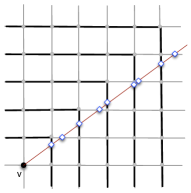
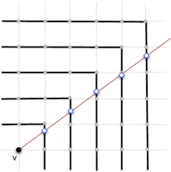
(a)	(b)

Figure 7: (a) The gridlines model: visibility is determined by the intersections of the LOS with all the grid lines. (b) The layers model: visibility is determined by the intersections of the LOS with the layers.

General idea and comparison to previous algorithms. Our algorithms vis-dac and vis-iter use an overall approach that is a combination of our radial sweep algorithm (Section 2) which partitions the grid into bands, and our centrifugal sweep algorithm (Section 4) which traverses the grid in layers around the viewpoint and maintains the horizon of the region traversed so far.

• Recall that the radial sweep algorithm from Section 2 consists of three phases: (1) partition the elevation grid in bands; (2) rotate the ray and compute visibility bands; (3) sort the visibility bands into a visibility grid. Phase 2 accesses data sequentially from all bands while the ray rotates around the viewpoint. The width of a band is chosen $w=\Theta(\sqrt{M})$. Our algorithms vis-iter and vis-dac have the same first and third phase, but in phase (2) they process the bands one at a time. The size of a band is set so that a band fits fully in memory.

• The centrifugal sweep algorithm Section 4 uses horizons which are stored discretized in an array. Our algorithms vis-iter and vis-dac use linear interpolation and therefore horizons are piecewise-linear functions and are stored as a list of $\{azimuth,zenith\}$ pairs with full precision.

We start by describing how to compute viewsheds in the layers model in Section 5.1 and 5.2; in Section 5.3 we show how our algorithms can be extended to the gridlines model while maintaining the same worst-case complexity.

5.1 An iterative algorithm: vis-iter

This section describes our first viewshed algorithm in the layers model, vis-iter. The main idea of vis-iter is to traverse the grid in layers around the viewpoint, one layer at a time, while maintaining the horizon of the region traversed so far. The horizon is maintained as a sequence of points $(t,H_{v}(t))$, sorted by $t$-coordinate, between which we interpolate linearly. When traversing a point $p$, the algorithm uses the maintained horizon to determine if $p$ is visible or invisible. In order to do this IO-efficiently, it divides the grid in bands around the viewpoint and processes one band at a time. The output visibility grid is generated band by band, and is sorted into a grid in the final phase of the algorithm. The size of the band is chosen such that a band fits in memory. Below we explain these steps in more detail.

Notation. The notation is the same as before and we review it for clarity: we ssume that the viewpoint $v$ is in the center of the grid at coordinates $(0,0,0)$ and the grid has size $(2m+1)\times(2m+1)$, where $m=(\sqrt{n}-1)/2$. The elevations of the grid points are given in a two-dimensional matrix $Z$ that is ordered row by row, with rows numbered from $-m$ to $m$ from north to south, and columns numbered from $-m$ to $m$ from west to east. By $p(i,j)$ we denote the grid point $q=(q_{x},q_{y},q_{z})$ in row $i$ and column $j$ with coordinates $q_{x}=j,q_{y}=-i$ and $q_{z}=Z_{ij}$.

For $l\geq 0$, let layer $l$ of the grid, denoted $L_{l}$, denote the set of grid points whose $L_{\infty}$-distance from the viewpoint, measured in the horizontal plane, is $l$. By definition, $L_{0}$ consists of only one point, $v$. We divide the grid in concentric bands around the viewpoint: For $k>0$, band $k$, denoted $B_{k}$, contains all points in layers $w_{k-1}$ (inclusive) to $w_{k}$ (exclusive), where $w_{k}(k\geq 0)$ denote the indices of layers corresponding to the band boundaries. Thus band $B_{1}$ contains all points in layers $w_{0}=1$ to $w_{1}$, and so on.

The algorithm starts with a preprocessing step which, given an arbitrary constant $K$, computes the band boundaries $w_{k}(k\geq 1)$ such that a band has size $\Theta(K)$ as follows: it cycles through each layer $i$ in the grid, computes (analytically) the number of points in that layer, and checks whether including this layer in the current band makes the band go over $K$ points. If yes, then layer $i$ marks the start of the next band. Otherwise, it adds the points in layer $i$ to the current band and continues.

The maximum size $K$ of a band is chosen such that a band fills roughly a constant fraction of memory, and each band is at least one layer wide. More precisely, we choose $K=c_{1}M$ and assume $\sqrt{n}\leq c_{1}M$, for a sufficiently small constant $c_{1}$ which will be defined more precisely later. Thus the number of bands, $N_{bands}$, is $O(N/M)$.

Once the band boundaries are set, the algorithm proceeds in three phases. The first phase is to generate, for each band $B_{k}$, a list $E_{k}$ containing the elevations of all points in the band. It does this by scanning the grid in row-column order: for each point $p(i,j)$, it calculates the index $k$ of the band that contains the point and writes $Z_{ij}$ to $E_{k}$. We note that the first phase writes the lists $E_{k}$ sequentially, and thus list $E_{k}$ contains the points in the order in which they are encountered during the (row-by-row) scan of the grid. The algorithm is given below.

Algorithm BuildBands:
load list containing band boundaries in memory
for $k\leftarrow 1$ to $N_{bands}$
do initialize empty list $E_{k}$
for $i\leftarrow-m$ to $m$
do for $j\leftarrow-m$ to $m$
do do read next elevation $Z_{ij}$ from grid
do do $k\leftarrow\textrm{band containing point }(i,j)$
do do append $Z_{ij}$ to $E_{k}$

Given the lists $E_{k}$, the second phase of the algorithm computes which points are visible. To do this it traverses the grid one band at a time, reading the list $E_{k}$ into memory. Once a band is in memory, it traverses it layer by layer from the viewpoint outward, counter-clockwise in each layer. The output of the second phase is a set of lists $V_{k}$ with visibility values, one list for each band. While traversing the grid in this fashion the algorithm maintains the horizon of the region encompassed so far. More precisely, let $L_{1,i}(i\geq 1)$ denote the set of points in layers $L_{1}$ through $L_{i}$. Before traversing the next layer $L_{i+1}$, the algorithm knows the horizon $H_{1,i}$ of $L_{1,i}$. While traversing the points in $L_{i+1}$, the algorithm determines for each point $p$ if it is above or below the horizon $H_{1,i}$ and records this in $V_{k}$. At the same time it updates $H_{1,i}$ on the fly to obtain $H_{1,i+1}$. To do so, the algorithm computes, for each point $p$, the projection $h$ onto the view screen of the line segment that connects $p$ to the previous point in the same layer, the algorithm computes the intersection of $h$ with the current horizon as represented by $H_{1,i}$, and then updates $H_{1,i}$ to represent the upper envelope of the current horizon and $h$. After traversing the entire grid in this manner, the set of points that have been marked visible during the traversal constitute the viewshed of $v$. The algorithm is given below only for the first octant; the other octants are handled similarly:

Algorithm VisBands-ITER:
$H_{1,0}\leftarrow\emptyset$
for $k\leftarrow 1$ to $N_{bands}$
do load list $E_{k}$ in memory
do create list $V_{k}$ in memory and initialize it as all invisible
do for $l\leftarrow w_{k-1}$ to $w_{k}$ //for each layer in the band
do do //traverse layer $l$ in ccw order
do do for $r\leftarrow 0$ to $-l$ //first octant
do do do get elevation $Z_{rl}$ of $p(r,l)$ from $E_{k}$
do do do determine if $Z_{rl}$ is above $H_{1,l-1}$
do do do if visible, set value $V_{rl}$ in $V_{k}$ as visible
do do do $h\leftarrow$ projection of $p(r-1,l)p(r,l)$
do do do merge $h$ into horizon $H_{1,l-1}$
do do $H_{1,l}\leftarrow H_{1,l-1}$

The third and final phase of the algorithm creates the visibility grid $V$ from the lists $V_{k}$. We note that in phase 2 the lists $V_{k}$ are stored in the same order as $E_{k}$, that is, the order in which the points in the band are encountered during a row-by-row scan of the grid; keeping points in this order is convenient because it saves an additional sort, and in the same time this is precisely the order in which they are needed by phase 3. Phase 3 is the reverse of phase 1: for each point $(i,j)$ in the grid in row-major order, it computes the band $k$ where it falls, accesses list $V_{k}$ to retrieve the visibility value of point $(i,j)$, and writes this value to the output grid $V$. The crux in this phase is that it simply reads the lists $V_{k}$ sequentially. The algorithm is given below:

Algorithm CollectBands:
load list containing band boundaries in memory
initialize empty list $V$
for $i\leftarrow-m$ to $m$
do for $j\leftarrow-m$ to $m$
do do $k\leftarrow\textrm{band containing point }(i,j)$
do do get value $V_{ij}$ of point $(i,j)$ from $V_{k}$
do do append $V_{ij}$ to list $V$

Efficiency analysis of vis-iter. We now analyze each phase in vis-iter under the assumption that $n\leq cM^{2}$ for a sufficiently small constant $c$. The pre-processing phase runs in $O(n)$ time and no I/O (does not access the grid). The output of this step is a list of $O(N_{bands})=O(n/M)$ band boundaries, which fits in memory assuming that $n\leq cM^{2}$ for a sufficiently small constant $c$.

The first phase, BuildBands, reads the points of the elevation grid in row-column order, which takes $O(n)$ time and $O(\mathsf{scan}(n))$ I/Os. With the list of band boundaries in memory, the band containing a point $(i,j)$ can be computed with, for example, binary search in $O(\lg n/M)=O(\lg n)$ time and no I/O. The lists $E_{k}$ are written to in sequential order. If one block from each band fits in memory, which happens when $n\leq cM^{2}/B$ for a sufficiently small constant $c$ (so that $N_{bands}=O(n/M)=O(M/B)$), then writing the lists $E_{k}$ directly takes $O(\mathsf{scan}(n))=O(\mathsf{sort}(n))$ I/Os (note that $O(\mathsf{sort}(n))$ and $O(\mathsf{scan}(n))$ are equal if $n=O(M^{2}/B)$). If we cannot keep one block of each band in memory, that is, $n>cM^{2}/B$, then we perform a hierarchical distribution as follows: we group the $N_{bands}$ bands in $O(M/B)$ super-bands, keep a write buffer of one block for each super-band in memory, distribute the points in the grid to these super-bands, and recurse on the super-bands to distribute the grid points to individual bands. A pass takes $O(\mathsf{scan}(n))$ I/Os, overall it takes $O(\log_{M/B}N_{bands})=O(\log_{M/B}N/M)$ passes, and thus the first phase has I/O-complexity $O(\mathsf{sort}(n))$. In total, the first phase takes $O(n\lg n)$ time and $O(\mathsf{sort}(n))$ I/Os.

The second phase, VisBands-ITER, takes as input the lists $E_{k}$ and computes the visibility bands $V_{k}$. We choose $K=c_{1}M$ such that the elevations $E_{k}$ and the visibility map $V_{k}$ of any band $B_{k}$ of size $K$ fits in 2/3 of the memory; the remaining 1/3 of the memory is saved for the horizon structure. While processing a band $B_{k}$ in the second phase, the points in $E_{k}$ and $V_{k}$ are not accessed sequentially. However, given the band boundaries, the location of any point in a band can be determined analytically, and thus the value (elevation or visibility) of any point in a band can be accessed in constant time, without any search structure, and without any I/O. Let us denote by $H_{tot}$ the total cumulative size of all partial horizons $H_{1,l}$: $H_{tot}=\sum_{l=1}^{\sqrt{n}}|H_{1,l}|$. The horizon $H_{1,l}$ is maintained as a list $\{(t,h)\}$ of horizontal and vertical coordinates on the view screen, sorted counter-clockwise (ccw) around the viewpoint. As the algorithm traverses a layer $l$ in ccw order, it also traverses $H_{1,l-1}$ in ccw order, and constructs $H_{1,l}$ in ccw order. To determine whether a point is above the horizon, it is compared with the last segment in the horizon; if the point is above the horizon, it is added to the horizon. Thus the traversal of a layer $l$ runs in $O(|L_{l}|+|H_{1,l-1}|+|H_{1,l}|)$ time. Over the entire grid, phase 2 runs in $O(\sum_{l}(|L_{l}|+|H_{1,l}|))=O(n+H_{tot})$ time. The IO-complexity of the second phase: The algorithm reads $E_{k}$ into memory, and writes $V_{k}$ to disk at the end. Over all the bands this takes $O(\mathsf{scan}(n))$ I/Os. If the horizon $H_{1,l}$ is small enough so that it fits in memory (for any $l$), then accessing the horizon does not use any IO. If the horizon does not fit in memory, we need to add the cost of traversing the horizon in ccw order, for every layer, $O(\mathsf{scan}(\sum_{l=1}^{\sqrt{n}}|H_{1,l}|))=\mathsf{scan}(H_{tot})$ I/Os.

Finally, the third phase, CollectBands, takes as input the lists $V_{k}$ and the list of band boundaries and writes the visibility map. For $n\leq cM^{2}$, the list of band boundaries fits in memory. For any point $(i,j)$ the band containing it can be computed in $O(\lg n)$ time and no IO. The bands $V_{k}$ store the visibility values in the order in which they are encountered in a (row-column) traversal of the grid. Thus, once the index $k$ of the band that contains point $(i,j)$ is computed, the visibility value of this point is simply the next value in $V_{k}$. As with step 1, we distinguish two cases: if the number of bands is such that one block from each band fit in memory, then this step runs in $O(n)$ time and $O(\mathsf{sort}(n))=O(\mathsf{scan}(n))$ I/Os. Otherwise, this step first performs a multi-level $M/B$-way merge of the bands into $O(M/B)$ super-bands so that one block from each can reside in main memory; in this case, the complexity of the step is $O(n\lg n)$ time and $O(\mathsf{sort}(n))$ I/Os. Putting everything together, we have the following:

Theorem 5.1

The algorithm vis-iter computes viewsheds in the layers model in $O(n\lg n+H_{tot})$ time and $O(\mathsf{sort}(n)+\mathsf{scan}(H_{tot}))$ I/Os, provided that $n\leq cM^{2}$ for a sufficiently small constant $c$.

Furthermore, if $n=O(M^{2}/B)$ and the partial horizons $H_{1,l}$ are small enough to fit in memory for any $l$, the overall IO complexity becomes $O(\mathsf{scan}(n))$ I/Os. We note that when $n=\Omega(M^{2})$ the algorithm can be adapted using standard techniques to run in the same bounds from Theorem 5.1; we do not detail on this because it has no relevance in practice.

Discussion. Phase 1 and 3 of the algorithm are very simple and perform a scanning pass over the grid and the bands, provided that $n\leq cM^{2}/B$: Phase 1 reads the input elevation grid sequentially and writes the elevation bands sequentially; Phase 3 reads the visibility bands sequentially and writes the visibility grid sequentially. We found this condition to be true in practice on our largest test grid ($28GB$) and with as little as $.5GB$ of RAM. With more realistic value of $M=8GB$ (and $B=16KB$), the condition is true for $n$ up to $10^{15}$ points. Thus, handling the sub-case $n\leq cM^{2}/B$ separately in the algorithm provides a simplification and a speed-up without restricting generality.

Phase 2, which scans partial horizons $H_{1,l}$ for every layer, runs in $O(n+H_{tot})$ time and $O(\mathsf{scan}(n+H_{tot}))$ I/Os. As we will prove below, in the worst case $|H_{1,l}|=\Theta(l^{2})$, and the running time of the second phase could be as high as $O(H_{tot})=O(\sum_{l=1}^{O(\sqrt{n})}\Theta(l^{2}))=O(n\sqrt{n})$, with handling the horizon dominating the running time. The worst-case complexity is high but, on the other hand, if $H_{1,l}$ are small, they fit in memory and the algorithm is fast. In particular if $H_{tot}$ is $O(n)$, then phase 2 is linear. This seems to be the case on all terrains and all viewpoints that we tried and may be a feature of realistic terrains. In Section 6 we’ll discuss our empirical findings in more detail.

Worst-case complexity of the horizon. Since the horizon is the upper envelope of the projections of grid line segments onto the view screen, its complexity is at most $O(n\alpha(n))$, where $n$ is the number of line segments [Hart and Sharir (1986), Wiernik and Sharir (1988)]. We will now show that we can prove a better bound for our setting. Let the width $\mathrm{width}(s)$ of a line segment $s$ be the length of its projection on a horizontal line. We need the following lemma.

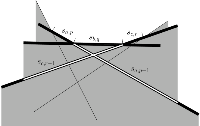
Figure 8: Illustration of the proof of Lemma 5.2. The white subsegments take the charge for $s_{b,q}$; together they are at least as wide as $s_{b}$, since they stick out from under $s_{b}$ on both sides.

Lemma 5.2

If $S$ is a set of $n$ line segments in the plane, such that the widths of the line segments of $S$ do not differ in length by more than a factor $d$, then the upper envelope of $S$ has complexity $O(dn)$.

Proof.

Let $s_{1},...,s_{n}$ be the segments of $S$. Each segment $s_{i}$ consists of a number of maximal subsegments such that the interior of each subsegment lies either entirely on or entirely below the upper envelope. Let the subsegments of $s_{i}$ be indexed by $s_{i,j}$, such that the subsegments of $s_{i}$ from left to right are indexed by consecutive values of $j$, and such that $s_{i,j}$ is part of the upper envelope if and only if $j$ is odd. Let $u_{1},...,u_{m}$ be the line segments of the upper envelope.

We consider two categories of line segments on the upper envelope: (i) segments that have at least one endpoint that is an endpoint of a segment of $S$; (ii) segments whose endpoints are no endpoints of segments in $S$.

Clearly, there can be only $O(n)$ segments of category (i), one segment to the left of each endpoint of a segment in $S$ and one segment to the right of each endpoint.

We analyze the number of segments of category (ii) with the following charging scheme. Given a segment $u_{h}=s_{b,q}$ of category (ii), let $s_{a,p}$ be the segment $u_{h-1}$ and let $s_{c,r}$ be the segment $u_{h+1}$. We charge $u_{h}$ to $s_{a,p+1}$ and $s_{c,r-1}$. Observe that with this scheme, each segment $s_{i,j}$ can only be charged twice, namely by the successor of $s_{i,j-1}$ on the upper envelope and by the predecessor of $s_{i,j+1}$ on the upper envelope. Since each segment $s_{i}$ has only one leftmost and only one rightmost subsegment, and each is charged at most twice (in fact, once), there are at most $O(n)$ segments of category (ii) that put charges on leftmost or rightmost subsegments. If neither $s_{a,p+1}$ is the rightmost subsegment of $s_{a}$ nor $s_{c,r-1}$ is the leftmost subsegment of $s_{c}$, then $s_{a}$ must appear on the upper envelope again somewhere to the right of the right end of $s_{b}$, and $s_{c}$ must appear on the upper envelope again somewhere to the left of the left end of $s_{b}$ (see Figure 8) Therefore $\mathrm{width}(s_{a,p+1})+\mathrm{width}(s_{c,r-1})>\mathrm{width}(s_{b})\geq\frac{1}{dn}\sum_{i=1}^{n}\mathrm{width}(s_{i})$. Since each subsegment is charged at most twice, the total length of subsegments charged is at most $2\sum_{i=1}^{n}\mathrm{width}(s_{i})$. Thus there are less than $2dn$ segments of category (ii) that put charges on subsegments that are not leftmost or rightmost. ∎

Note that the widths of the projections of the edges of layer $l$ on the view screen vary between $1/(l+1)$ and $1/(4l-2)$. Therefore, the widths of the projections of the edges of the $l/2$ outermost layers in a square region of $l$ layers around $v$ differ by less than a factor 8. Thus, from Lemma 5.2 we get:

Corollary 5.3

If $S$ consists of the $O(l^{2})$ edges of the $l/2$ outermost layers in a square region of $l$ layers around $v$, then the horizon of $S$ has complexity $O(l^{2})$.

Lemma 5.4

If $S$ and $T$ are two $x$-monotone polylines of $m$ and $n$ vertices, respectively, then the upper envelope of $S$ and $T$ has at most $2(m+n)$ vertices.

Proof.

There are two types of vertices on the upper envelope: vertices of $S$ or $T$, and intersection points between edges of $S$ and $T$. Clearly, there are at most $m+n$ vertices of the first type. Between any pair of vertices of the second type, there must be a vertex of the first type. Thus there are at most $m+n-1$ vertices of the second type. ∎

Theorem 5.5

If $S$ consists of $l$ layers in a square region around $v$, then the horizon of $S$ has complexity $O(l^{2})$ in the worst case.

Proof.

Let $T(l)$ be the complexity of the horizon of the innermost $l$ layers around $S$. By Lemma 5.4, $T(l)$ is at most twice the complexity of the horizon of the innermost $l/2$ layers, plus twice the complexity of the remaining $l/2$ layers. By Corollary 5.3, the latter is $O(l^{2})$, and therefore we have $T(l)\leq 2T(l/2)+O(l^{2})$. This solves to $T(l)=O(l^{2})$. ∎

5.2 A refined algorithm: vis-dac

This section describes our second algorithm for computing viewsheds in the layers model, vis-dac. vis-dac is a divide-and-conquer refinement of vis-iter and uses the same general steps: it splits the grid into bands, computes visibility one band at a time, and creates the visibility grid from the bands. The first phase (BuildBands) and last phase (CollectBands) are the same as in vis-iter; the only phase that is different is computing visibility in a band, VisBands-DAC, which aims to improve the time to merge horizons in a band using divide-and-conquer.

Similar to VisBands-Iter, VisBands-DAC processes the bands one at a time: for each band $k$ it loads list $E_{k}$ in memory, creates a visibility list $V_{k}$ and initializes it as all visible. It then marks as invisible all points that are below $H_{prev}$, where $H_{prev}$ represents the horizon of the first $k-1$ bands (more on this below). The bulk of the work in visBands-DAC is done by the recursive function Dac-Band, which computes and returns the horizon $H$ of $E_{k}$, and updates $V_{k}$ with all the points that are invisible inside $E_{k}$. This is described in detail below. Finally, the horizon $H$ is merged with $H_{prev}$ setting it up for the next band.

In order to mark as invisible the points in band $k$ that are below $H_{prev}$ we first sort the points in the band by azimuth angle and then scan them in this order while also scanning $H_{prev}$ (recall that $H_{prev}$ is stored in ccw order). Let $(a_{1}=0,h_{1}),(a_{2},h_{2})$ be the first two points in the horizon $H_{prev}$. For every point $p=(a,h)$ in $E_{k}$ with azimuth angle $a\in[a_{1},a_{2}]$, we check whether its height $h$ is above or below the height of segment $(a_{1},h_{1})(a_{2},h_{2})$ in $H_{prev}$. When we encounter a point in $E_{k}$ with $a>a_{2}$, we proceed to the next point in $H_{prev}$ and repeat.

The recursive algorithm DAC-Band takes as arguments an elevation band $E_{k}$, a visibility band $V_{k}$, and the indices $i$ and $j$ of two layers in this band ($w_{k-1}\leq i\leq j<w_{k}$). It computes visibility for the points in layers $i$ through $j$ (inclusive) in this band, and marks in $V_{k}$ the points that are determined to be invisible during this process. In this process it also computes and returns the horizon of layers $i$ through $j$ in this band. Dac-Band uses divide-and-conquer in a straightforward way: first it computes a “middle” layer $m,i\leq m\leq j$ between $i$ and $j$ that splits the points in layers $i$ through $j$ approximately in half. Then it computes visibility and the horizon recursively on each side of $m$; marks as invisible all points in the second half that fall below the horizon of the first half; and finally, merges the two horizons on the two sides and returns the result.

Algorithm Dac-Band($E_{k},V_{k},i,j$):
if $i==j$
if $h\leftarrow$ compute-layer-horizon(i)
if return $h$
else
else $m\leftarrow$ middle layer between $i$ and $j$
else $h_{1}\leftarrow\textsc{Dac-Band}(E_{k},V_{k},i,m)$
else $h_{2}\leftarrow\textsc{Dac-Band}(E_{k},V_{k},m+1,j)$
else mark invisible all points in $L_{m+1,j}$ that fall below $h_{1}$
else $h\leftarrow$ merge($h_{1},h_{2}$)
else return $h$

Efficiency analysis of vis-dac. The analysis of the first and last phase of vis-dac, buildBands and CollectBands, is the same as in Section 5.1. We now analyze VisBands-DAC. Recall that we can assume that $E_{k}$ and $V_{k}$ both fit in memory during this phase (see Section 5.1). The elevation and visibility of any point in a band can be accessed in $O(1)$ time, without any search structure and without any I/O. We denote $H^{B}_{1,i}$ the horizon of (the points in) the first $i$ bands; and by $H^{B}_{tot}=H^{B}_{1,1}+H^{B}_{1,2}+H^{B}_{1,3}+...=\sum_{i=1}^{N_{bands}}H^{B}_{1,i}$.

• Marking as invisible the points in $E_{k}$ that are below $H_{prev}$ (here $H_{prev}$ represents $H^{B}_{1,k-1}$): this can be done by first sorting $E_{k}$ and then scanning $H^{B}_{1,k-1}$ and $E_{k}$ in sync. Over the entire grid, this takes $O(n\lg n+H^{B}_{tot})$ CPU and $O(\mathsf{scan}(n)+\mathsf{scan}(H^{B}_{tot}))$ I/Os.

• Merging horizons: After Dac-band is called in a band, the returned horizon is merged with $H_{prev}$. Two horizons can be merged in linear time and I/Os. Over the entire grid this is $O(H^{B}_{tot})$ time and $O(\mathsf{scan}(H^{B}_{tot}))$ I/Os.

• Dac-band: This is a recursive function, with the running time given by the recurrence $T(k)=2T(k/2)+\texttt{merge cost + update cost}$, where $k$ is the number of points in the slice between layers $i$ and $j$ given as input. The base case computes the horizon of a layer $l$, which takes linear time wrt to the number of points in the layer. Summed over all the layers in the slice the base case takes $O(\sum_{l=i}^{j}|L_{l}|)=O(k)$ time and no I/O (band is in memory).

• The update time in Dac-band represents the time to mark as invisible all points in the second half that fall below the horizon $h_{1}$ of the first half. Recall that a band fits in memory and thus an input slice in Dac-Band fits in memory. If the band is sorted, the update can be done as above in $O(k+|h_{1}|)=O(k)$ time (by Theorem 5.5 we have $|h_{1}|=O(k)$).

• The merge time in Dac-band represents the time to merge the horizons $h_{1}$ and $h_{2}$ of the first and second half of the slice, respectively. This takes $O(|h_{1}|+|h_{2}|)=O(k)$ time.

• Putting it all together in the recurrence relation we get $T(k)=2T(k/2)+O(k)$, which solves to $O(k\lg k)$ time. Summed over all bands in the grid Dac-Band runs in $O(n\lg n)$ time and $O(\mathsf{scan}(n))$ I/Os.

Overall we have the following:

Theorem 5.6

The algorithm vis-dac computes viewsheds in the layers model in $O(n\lg n+H^{B}_{tot})$ time and $O(\mathsf{sort}(n)+\mathsf{scan}(H^{B}_{tot}))$ I/Os, provided that $n\leq cM^{2}$, for a sufficienly small constant $c$.

Discussion: The worst case complexity of $H^{B}_{tot}$ is $\sum_{i=1}^{N_{bands}}H^{B}_{1,i}=O(N_{bands}\cdot n)=O(n^{2}/M)$; This is an improvement over $O(n\sqrt{n})$ ( provided that $n\leq cM^{2}$). Consider a band that extends from layer $L_{i}$ to layer $L_{j}$ and contains $k$ points. The algorithm Dac-Band runs in $O(k\lg k)$ time, while the iterative algorithm VisBands-Iter scans iteratively through all cumulative horizons of the layers in the band $H_{1,i},H_{1,i+1},...$ and so on and runs in $O(k+|H_{1,i}|+|H_{1,i+1}|+...+|H_{1,j}|)$. When the horizons are small, vis-iter runs in $O(k)$ time and is faster than vis-dac. The divide-and-conquer merging is not justified unless the horizons are large enough to benefit from it.

5.3 The gridlines model

The algorithms vis-dac and vis-iter described in Section 5.1 and 5.2 above compute viewsheds in the layers model. Let $X_{i}$ denote the line segments connecting points at distance $i-1$ with points at distance $i$ (Figure 9). The set $X_{i}$ represents the additional “obstacles” in the $i$th layer that could intersect the LOS in the gridlines model. With this notation the horizon of the $i$th layer in the gridlines model is $H(L_{i})\cup H(X_{i})$. The algorithms vis-iter and vis-dac can be extended to compute viewsheds in the gridlines model—the only difference is that they compute the horizon of a layer as $H(L_{i})\cup H(X_{i})$ instead of $H(L_{i})$. Since $|X_{i}|=\Theta(|L_{i}|)$, the analysis and the bounds of the algorithms are the same in both models up to a constant factor. Our algorithms vis-iter and vis-dac, when using the gridlines model, compute the same viewshed as R3 [Franklin and Ray (1994)]. vis-dac’s upper bound of $O(n\lg n+n^{2}/M)$ is an improvement over R3’s bound of $O(n\sqrt{n})$, provided that $n\leq cM^{2}$.

The results on the worst-case complexity of the horizon in the layer model extend to the gridlines model. The extension is not entirely straightforward, because the differences in width in the projection between non-layer edges are larger than between layer edges. We defer the proof to the journal version of this paper.

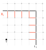
Figure 9: The segments contributing to a layer’s horizon in the gridlines model

6 Experimental results

In this section we describe the implementation details and the results of the experiments with our algorithms. We implemented the five algorithms described above: io-radial2 is the layered radial sweep algorithm described in Section 2; io-radial3 is the radial sweep algorithm from Section 3; io-centrifugal is the centrifugal sweep algorithm from Section 4; vis-iter and vis-dac are the two algorithms described in Section 5.2 and 5.1, respectively. We use as reference the algorithm from our previous work, io-radial1 [Haverkort et al. (2008)], which is also based on Van Kreveld’s model.

6.1 Implementation details

We start by reviewing the implementation details of our algorithms.

io-radial1 scans the elevation grid, creates 3 events for each cell and writes them to the event stream; with 12 bytes per event, the event stream is $36n$ bytes. It then sorts the event stream by azimuth angle. To sweep, it scans the event stream in order while using an active structure to keep track of the events that intersect the sweep line. During the sweep, the cells that are visible are written to a file. In the end, the file is sorted by location and written to the output grid. io-radial1 can function in a recursive mode if it determines that the active structure does not fit in memory. However in all datasets the active structure is small ($<$30 MiB) and completely fits in memory [Haverkort et al. (2008)].

io-radial2 performs 2 passes over the elevation grid. It first maps the elevation grid file in (virtual) memory and creates the sorted layers $E_{k}$. During this phase, the elevation grid and the sorted arrays $E_{k}$ are kept in memory, and io-radial2 relies on the virtual memory manager (VMM) to page in blocks from the elevation grid as necessary when accessing the points in band $k$. Note that the accesses to the elevation grid are not sequential (although they amount to $O(\mathsf{scan}(n))$ I/Os). To help the VMM we implemented the following strategy: whenever the current band needs to access an elevation from the grid, we load an entire square tile of $\Theta(M)$ points in memory, and keep track of the two most recent tiles. Once all $E_{k}$ are computed the elevation grid is freed. During the second phase (the sweep) the elevations are accessed sequentially from the bands $E_{k}$ and the output grid is kept in (virtual) memory as a bitmap grid.

io-radial3 also performs 2 (sequential) passes over the elevation grid. The first pass scans over the elevation grid and places each point $(i,j,Z_{ij})$ in its sector. Sectors are stored as streams on disk. The second pass sorts and sweep the points in one sector at a time by $\textsc{enter}(i,j)$. The output grid is kept in (virtual) memory as a bitmap grid. Except for the output grid, io-radial3 does not use the VMM.

io-radial1, io-radial2 and io-radial3 use the same data structures: a heap as a priority queue; a red-black tree for the active structure [Cormen et al. (2001)]; and the same in-memory sorting (optimized quicksort). For the largest terrains the priority queue and the active structure are at most 30MB and fit in memory.

io-centrifugal is implemented in one (non-sequential) pass over the elevation grid. The implementation is recursive, as described in Section 4. Theoretically the algorithm could run completely cache-obliviously with help of the VMM, but this turned out to be slow. Therefore we implemented a cache-aware version: whenever the recursion enters a tile $G$ of the largest size that fits in memory, we load the elevation values for the entire tile into memory; when the algorithm returns from the recursive call on $G$, the visibility values for $G$ are written to disk.

vis-iter performs two sequential passes over the elevation grid, and one over the visibility grid. The first pass reads the elevation grid and creates the bands, and the second pass loads the bands one by one in memory and computes the visibility bands. The horizon is maintained as an array of (azimuth, zenith) pairs, and is accessed sequentially; in all our experiments it never exceeded 200,000 points.

vis-dac implements a divide-and-conquer refinement of vis-iter. When when a band is loaded in memory, vis-dac will compute and merge the layers in the band in a way similar to mergesort, which leads to an improved upper bound for its time complexity. vis-dac and vis-iter share the same code. The user can switch between the two by turning on or off a flag that triggers the divide-and-conquer. There is another flag to select the model (gridlines or layers).

The implementations of all of our algorithms avoid taking square roots and arctangents, and do not store any angles. Instead of elevation angles, they use the signed squared tangents of elevation angles, and instead of azimuth angles, they use tangents of azimuth angles relative to the nearest axis direction (north, east, south, or west).

6.2 Platform

The algorithms are implemented in C and compiled with gcc/g++ 4.1.2 (with optimization level -O3). All experiments were run on HP 220 blade servers, with an Intel 2.83 GHz processor and a 5400 rpm SATA hard drive (the HP blade servers come only with this HD option). The machine is quad-core, but only one CPU was used. We ran experiments rebooting the machine with 512 MiB and 1 GiB of RAM. These sizes do not reflect current technology, and have been chosen in order to emphasize the scalability of the algorithms to a volume of data that is much larger than the amount of RAM available.

6.3 Datasets

The algorithms were tested on real terrains ranging up to over 7.6 billion elements, see Table 1 for some examples. The largest datasets are SRTM1 data, 30m resolution, available at http://www2.jpl.nasa.gov/srtm/.We selected these datasets because they are easily available, and are large. In practice it does not make sense to compute a viewshed on a very large area at low resolution; instead we would want to use a grid corresponding to a relatively small area at high resolution. We used SRTM data because it was easily and freely available, and served our goal to compare the algorithms.

On all datasets up to 4 GiB (Washington), viewshed timings were obtained by selecting several viewpoints uniformly on each terrain and taking the average time. For the larger datasets we chose a viewpoint approximately in the middle of the terrain. This gives a good indication of the algorithm’s performance, and we note that for all our algorithms the majority of the running time is spent handling the bands, and we expect that the total runing time will vary insignificantly with the position of the viewpoint.

Dataset	Size
	cols $\times$	rows	GiB
Cumberlands	8 704 $\times$	7 673	0.25
USA DEM 6	13 500 $\times$	18 200	0.92
USA DEM 2	11 000 $\times$	25 500	1.04
Washington	31 866 $\times$	33 454	3.97
SRTM1-region03	50 401 $\times$	43 201	8.11
SRTM1-region04	82 801 $\times$	36 001	11.10
SRTM1-region06	68 401 $\times$	111 601	28.44

Table 1: Sample datasets

6.4 Results

Figure 10 shows the total running times of all our algorithms with 512 MiB RAM. First, we note that all our algorithms, being based on I/O-efficient approaches, are scalable to data that is more than sixty times larger than the memory of the machine. This is in contrast with the performance of an internal-memory algorithm, which would start thrashing and could not handle terrains moderately larger than memory, as showed in [Haverkort et al. (2008)].

io-radial1, io-radial2 and io-radial3 are all based on radial sweeps of the terrain, and theoretically they all use $\Theta(\mathsf{sort}(n))$ I/Os. In practice, however, both our new algorithms are significantly faster than io-radial1. On Washington (3.97 GiB), io-radial1 runs in 32,364 seconds with 16% CPU, while io-radial2 runs in 13,780 seconds (22% CPU), and io-radial3 in 3,009 seconds (89% CPU). This is a speed-up factor of more than 10.

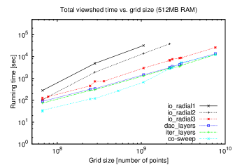
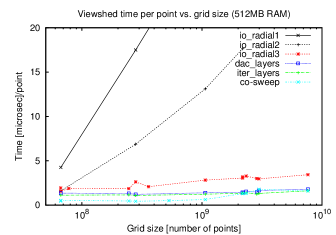
Figure 10: Running times with 512MB RAM. (a) Total time (log scale) with dataset size (log scale). (b) Total time per point.

Both io-radial2 and io-radial3 perform two passes over the elevation grid, however io-radial3 is much faster. On a machine with 512 MiB RAM, on SRTM-Region 3 (8.11 GiB), io-radial2 takes 37,982 seconds (16% CPU), while io-radial3 runs in 6,644 seconds (81% CPU). Overall, for io-radial2 roughly 20% of the time is CPU time, while for io-radial3 the CPU utilization is 80% or more. The difference may be explained by the fact that the first pass of io-radial2 is non-sequential (although it performs $O(n/B)$ I/Os), while both passes of io-radial3 are sequential. Another difference is that io-radial2 uses the VMM more than io-radial3.

Our third algorithm, io-centrifugal, is the fastest. It finishes a 28.4 GiB terrain (SRTM-Region 6) in 12,186 seconds (203 minutes), while io-radial2 takes 26,193 seconds (437 minutes). For io-radial3, 61% of this time is CPU time, while for io-centrifugal only 18%. The reason is that io-centrifugal does a single pass through the elevation grid. For any grid point $u$, the highest elevation angle of the $O(\sqrt{n})$ cells that may be on the line of sight from $v$ to $u$ is retrieved from the horizon array in $O(1)$ time, and the horizon array is maintained in $O(1)$ time per point on average. As a result, io-centrifugal is CPU-light and the bottleneck is loading the blocks of data into memory. io-radial3, on the other hand, is more computationally intensive—the highest elevation angle on the line of sight to $u$ needs to be retrieved from a red-black tree in $O(\log n)$ time, and that tree is maintained in $O(\log n)$ time per point. In addition, io-radial3 needs time to sort events.

One of our findings is that relying purely on VMM, even for a theoretically I/O-efficient data access, is slow. The analysis of the I/O-efficiency of both io-radial2 and io-centrifugal is based on the assumption that the VMM will automatically load tiles of size $\Theta(M)$ into memory in the optimal way, and that in practice the performance will not be very different (the theoretical foundations for this assumption were given by [Frigo et al. (1999)]). In practice this did not work out so well: a fully cache-oblivious, VMM-based implementation of io-centrifugal and io-radial2 turned out to be slow. By telling the algorithms explicitly when to load a memory-size block (and not using the VMM), we obtained significant speedups (without sacrificing I/O-efficiency for the levels of caching of which the algorithm remained oblivious, and without sacrificing CPU-efficiency). We believe that we could further improve the running time of io-centrifugal by having it manage the process of caching in memory the blocks of data that it needs to access from the grid on disk (write its own block manager with LRU policy).

Interestingly, our linear interpolation algorithms vis-iter and vis-dac are faster than io-radial3, and slightly slower than io-centrifugal. For all datasets we found that $n\leq cM^{2}/B$ for a sufficiently small constant $c$, which means that BuildBands and CollectBands run in a single pass over the data. Thus both algorithms perform two passes over the elevation grid, and a pass over the visibility grid to assemble to visibility bands. The total running time is split fairly evenly between the three phases. The actual visibility calculation runs at 100% CPU and represents $<$ 25% of the running time. More than 75% of the total time is spent reading or writing the bands.

In all our tests we found that the iterative algorithm vis-iter is consistently 10-20% faster than vis-dac. To understand this we investigated the size of the horizons computed by vis-dac and vis-iter: $H_{i}$, the horizon of layer $i$; and $H_{1,i}$, the horizon of the points in the first $i$ layers. Note that the number of grid points on level $i$ is $8i$, and the total number of points on levels $1$ through $i$ is $4i^{2}+4i+1=\Theta(i^{2})$. We know that $H_{i}=O(i)=O(\sqrt{n})$, and $H_{1,i}=O(i^{2})=O(n)$ (Theorem 5.5). We recorded $|H_{i}|$ and $|H_{1,i}|$ for each layer $i$ during the execution of vis-iter. Figure 11 shows the results for two datasets; the results for the other datasets look similar.

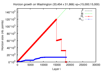
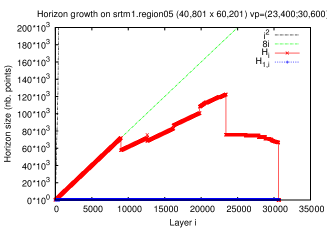
Figure 11: Horizon growth for a viewshed computation on datasets Washington and srtm1.region05

We see that $|H_{i}|$ is very close to its theoretical bound of $8i=\Theta(i)$. As $i$ gets larger the $i$th layers starts to fit only partially in the grid, and this causes $|H_{i}|$ to drop and have steep variations. The main finding is that for all datasets $H_{1,i}$ stays very small, far below its theoretical upper bound of $\Theta(i^{2})$. $H_{1,i}$ grows fast initially and then flattens out; For e.g. on Washington dataset (approx. 1 billion points), $|H_{1,i}|$ flattens at 13,452 points; and on srtm1.region05 (approx. 2.5 billion points), $|H_{1,i}|$ flattens at 460 points. All SRTM datasets have the horizon $H_{1,O(\sqrt{n})}$ between 132 and 32,689.

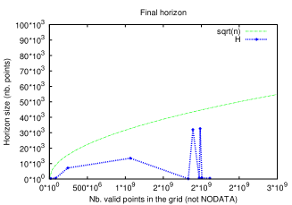
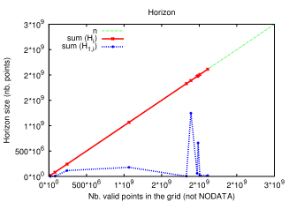
Figure 12: (a) Size of final grid horizon $|H_{1,O(\sqrt{n})}|$ with dataset size. (b) $\sum_{i=1}^{O(\sqrt{n})}|H_{1,i}|$ and $\sum_{i=1}^{O(\sqrt{n})}|H_{i}|$ with dataset size.

Given a dataset, we refer to the horizon $H_{1,O(\sqrt{n})}$ as its final horizon. Figure 12(a) shows the size of the final horizon for each dataset as function of the number of valid points in the grid —- this excludes the points in the grid that are labeled as nodata, and which are used for e.g. to label the water/ocean; these points do not affect the size of the horizon, as chains of nodata points are compressed into a single horizon segment. We see that the final horizon: (1) has a lot of variation especially for the larger SRTM datasets, jumping from low to high values. This is likely due to the position of the viewpoint and possibly the topology of the terrain; (2) the horizon stays small, below $\sqrt{n}$ for all datasets, far below its worst-case bound of $O(n)$.

Figure 12(b) shows the cumulative sums, $\sum_{i=1}^{O(\sqrt{n})}|H_{1,i}|$ and $\sum_{i=1}^{O(\sqrt{n})}|H_{i}|$, for each dataset, as a function of the number of valid points in the grid; we recorded these sums because they come up in the analysis of vis-iter and can shed light on its performance. In Figure 12 we see that $\sum_{i=1}^{O(\sqrt{n})}|H_{i}|$ grows indeed linearly with the number of valid points in the grid. The sum $\sum_{i=1}^{O(\sqrt{n})}|H_{1,i}|$ has a lot of variability similar with the final horizon shown in Figure 12 (a), and for all datasets stays far from its worst-case upper bound of $O(n\sqrt{n})$. We note that Figure 11 and 12 are based on a single viewpoint, but we expect the results will carry over.

Comparing to the work of Ferreira et al. [Ferreira et al. (2012)]: Their algorithm, TiledVS, also consists of three passes: convert the grid to Morton order, compute visibility using R2 algorithm, and convert the output grid from Morton order to row-major order. They report on the order of 5,000 seconds with TiledVS for SRTM1.region06, using a similar platform as ours and additional optimization like data compression. Assuming that this time includes all three passes, and modulo variations in setup, it is approx. 2.5 times faster than vis-iter. We note that TiledVS uses a different model and we believe our algorithms and their analysis are of independent interest.

7 Conclusion

In this paper we described new I/O-efficient algorithms for computing the visibility map of a point on a grid terrain using several different models. The algorithms are provably efficient in terms of the asymptotic growth behaviour of the number of I/Os, but at the same time are designed to exploit that the terrain model is a grid. This leads to much improved running times compared to our previous work [Haverkort et al. (2008)]. On the largest terrains, using as little as 512 MiB of memory, our algorithms perform at most two passes through the input data, and one pass through the output grid. We were able to compute viewsheds on a terrain of 28.4 GiB in 203 minutes with a laptop-speed hard-drive. The algorithms that compute (what is considered to be) the exact viewshed have inferior worst-case upper bounds, but in practice are faster than the radial-sweep algorithms due to the small size of horizons. We conclude that horizon-based algorithms emerge as a fast approach for computing viewsheds.

As avenues for future reesarch we mention the problem of proving a sub-linear bound for the expected complexity of a horizon, and obtaining an output-sensitive viewshed algorithm.

8 Acknowledgments

The authors thank DJ Merill for setting up and administering the platform used for the experiments. And former Bowdoin students Jeremy Fishman and Bob PoFang Wei for working on the earlier versions of this paper.

References

- Aggarwal and Vitter (1988) Aggarwal, A. and Vitter, J. S. 1988. The Input/Output complexity of sorting and related problems. Communications of the ACM 31, 9, 1116–1127.
- Andrade et al. (2011) Andrade, M. V. A., Magalhães, S. V. G., Magalhães, M. A., Franklin, W. R., and Cutler, B. M. 2011. Efficient viewshed computation on terrain in external memory. Geoinformatica 15, 2, 381–397.
- Brodal et al. (2007) Brodal, G. S., Fagerberg, R., and Vinther, K. 2007. Engineering a cache-oblivious sorting algorithm. J. Exp. Algorithmics 12, 2.2.
- Cole and Sharir (1989a) Cole, R. and Sharir, M. 1989a. Visibility problems for polyhedral terrains. J. Symb. Comput. 7, 1, 11–30.
- Cole and Sharir (1989b) Cole, R. and Sharir, M. 1989b. Visibility problems for polyhedral terrains. J. Symbolic Computation 7, 11–30.
- Cormen et al. (2001) Cormen, T. H., Leiserson, C. E., Rivest, R. L., and Stein, C. 2001. Introduction to Algorithms, second ed. The MIT Press, Cambridge, Mass.
- de Floriani and Magillo (1994) de Floriani, L. and Magillo, P. 1994. Visibility algorithms on digital terrain models. International Journal of Geographic Information Systems 8, 1, 13–41.
- de Floriani and Magillo (1999) de Floriani, L. and Magillo, P. 1999. Geographic Information Systems: Principles, Techniques, Managament and Applications. John Wiley and Sons, Chapter Intervisibility of Terrains, 543–556.
- Ferreira et al. (2012) Ferreira, C. R., Magalhães, S. V. G., Andrade, M., Franklin, W. R., and Pompermayer, A. M. 2012. More efficient terrain viewshed computation on massive datasets using external memory. In Proc. 20th ACM SIGSPATIAL Symp. Geographic Information Systems (GIS 2012). 169–172.
- Fishman et al. (2009) Fishman, J., Haverkort, H., and Toma, L. 2009. Improved visibility computations on massive grid terrains. In Proc. 17th ACM SIGSPATIAL Symp. Geographic Information Systems (GIS 2009). 121–130. Best paper award.
- Franklin and Ray (1994) Franklin, W. R. and Ray, C. 1994. Higher isn’t necessarily better: Visibility algorithms and experiments. In Proc. Symposium on Spatial Data Handling. 751–763.
- Frigo et al. (1999) Frigo, M., Leiserson, C. E., Prokop, H., and Ramachandran, S. 1999. Cache-oblivious algorithms. In Proc. IEEE Symposium on Foundations of Computer Science. 285–298.
- Hart and Sharir (1986) Hart, S. and Sharir, M. 1986. Nonlinearity of Davenport-Schinzel sequences and of generalized path compression schemes. Combinatorica 6, 151–177.
- Haverkort et al. (2013) Haverkort, H., Toma, L., and Wei, B. 2013. On io-efficient viewshed algorithms and their accuracy. In Proc. 21st ACM SIGSPATIAL Symp. Geographic Information Systems (GIS 2013). 24–33.
- Haverkort et al. (2008) Haverkort, H., Toma, L., and Zhuang, Y. 2008. Computing visibility on terrains in external memory. ACM Journal on Experimental Algorithmics 13, 1.5.1–1.5.23.
- Izraelevitz (2003) Izraelevitz, D. 2003. A fast algorithm for approximate viewshed computation. Photogrammetric Engineering and Remote Sensing 69, 7 (July), 767–774.
- van Kreveld (1996) van Kreveld, M. 1996. Variations on sweep algorithms: efficient computation of extended viewsheds and class intervals. In Proc. Symposium on Spatial Data Handling. 15–27.
- Wiernik and Sharir (1988) Wiernik, A. and Sharir, M. 1988. Planar realization of nonlinear Davenport-Schinzel sequences by segments. Discrete and Computational Geometry 3, 15–47.