Edge domain walls in ultrathin exchange-biased films

Abstract

We present an analysis of edge domain walls in exchange-biased ferromagnetic films appearing as a result of a competition between the stray field at the film edges and the exchange bias field in the bulk. We introduce an effective two-dimensional micromagnetic energy that governs the magnetization behavior in exchange-biased materials and investigate its energy minimizers in the strip geometry. In a periodic setting, we provide a complete characterization of global energy minimizers corresponding to edge domain walls. In particular, we show that energy minimizers are one-dimensional and do not exhibit winding. We then consider a particular thin film regime for large samples and relatively strong exchange bias and derive a simple and comprehensive algebraic model describing the limiting magnetization behavior in the interior and at the boundary of the sample. Finally, we demonstrate that the asymptotic results obtained in the periodic setting remain true in the case of finite rectangular samples.

1 Introduction

Ferromagnetic films and multilayers are fundamental nanostructures widely used in present day magnetoelectronics devices [39]. As such, they have been the subject of intensive investigations over the last two decades in the engineering, physics and applied mathematics communities [21, 1, 10, 15, 12]. Some of the highlights of these activities include the discoveries of giant magnetoresistance, spin-transfer torque, spin-orbit coupling and the spin-Hall effect [1, 4, 43, 17]. These new physical phenomena have lead to the design of such technological applications as magnetic sensors, actuators, high-density magnetic storage devices and non-volatile computer memory.

Surface and interfacial effects play a dominant role and are responsible for determining many properties of the nanostructured ferromagnetic materials [21, 10, 17]. These phenomena become increasingly important in the case of ultrathin films and multilayers. One basic example of such nanostructures is given by exchange-biased materials, which consist of a ferromagnetic film on top of an antiferromagnetic layer [36]. As a consequence of an exchange coupling between the two layers, the magnetization in the ferromagnetic film experiences a net bias induced by the magnetization at the interlayer interface, which furnishes the free layer with an effective unidirectional anisotropy. Additionally, nanostructure edges may also drastically change the equilibrium and the dynamic behaviors of the magnetization. For instance, the nanostructure edges often determine the mechanism of the magnetization reversal process [21, 14, 34]. However, despite the importance of edge effects there exist just a handful of rigorous analytical studies characterizing the magnetization behavior near the film edges [23, 25, 31, 27, 35].

Formation of edge domain walls is an important manifestation of edge effects observed in ferromagnetic films, double layers and exchange-biased materials [19, 20, 44, 41, 28, 9, 21, 10, 40]. Edge domain walls appear as the result of a competition between magnetostatic energy dominating near the edges and the anisotropy or bias field effects in the bulk, leading to a mismatch in the preferred magnetization directions near and far from the film edges. It is well known that in ultrathin ferromagnetic films without perpendicular magnetic anisotropy the magnetization prefers to stay almost entirely in the film plane. At the same time, the magnetization tends to stay parallel to the film edge even if the magnetocrystalline anisotropy or the bias field favor a different magnetization direction in the interior. This effect is due to the stray field energy which produces a significant contribution near the sample edges [23]. Inside the sample, the bias field and/or magnetocrystalline anisotropy dominate the micromagnetic energy, favoring a single domain state. When these effects are sufficiently strong, they may also influence the magnetization behavior close the sample boundary. As a result of the competition between the stray field and anisotropy/exchange bias energies, also taking into account the exchange energy, a transition layer near the edge, called edge domain wall, is formed. Although this simple phenomenological explanation gives an intuitive picture, apart from a few ansatz-based studies in the physics literature [19, 20, 37, 18] there is currently little quantitative understanding of this phenomenon.

The goal of this paper is to understand the formation of edge domain walls in exchange-biased materials, viewed as minimizers of the micromagnetic energy. We are interested in soft ultrathin ferromagnetic films in the presence of a strong exchange bias field. Our analysis is based on a reduced two-dimensional micromagnetic energy with magnetization vector constrained to lie in the film plane, which is well known to adequately describe the magnetization behavior in ultrathin ferromagnetic films [33, 23, 12]. Since we are concerned with the magnetization behavior near the edges, we consider one of the simplest and yet application relevant geometries, namely, that of a ferromagnetic strip. As described earlier, in this geometry the magnetization inside the strip aligns with the direction of the bias field, but at the edges it tends to align along the fixed edge direction. Typically, there is a misalignment between these two directions which, with the help of the exchange energy, results in the formation of a boundary layer near the edge (see Fig. 1). Let us stress that the situation considered here is very different from the case treated in [23], where the magnetization behavior at the boundary is controlled by the magnetization in the interior through the trace theorem. In larger ferromagnetic samples considered here the exchange energy does not impose enough control over magnetization variation. This results in the detachment of the trace of the interior magnetization profile from the magnetization at the sample boundary. In particular, the actual magnetization behavior at the boundary is determined in a non-trivial way through the competition of exchange bias, stray field and bulk exchange energies.

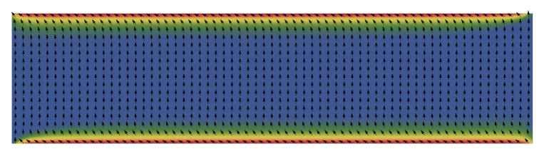
Figure 1: A remanent magnetization in an exchange-biased permalloy film (exchange constant $A=1.3\times 10^{-11}$ J/m, saturation magnetization $M_{s}=8\times 10^{5}$ A/m, exchange bias field $H=8.91\times 10^{3}$ A/m) with dimensions $3.46\mu$m$\times 0.87\mu$m$\times 6$nm. Result of a micromagnetic simulation, using the code developed in [33]. The bias field is pointing up. Edge domain walls exhibiting partial alignment of the magnetization with the sample edges may be seen at the top and the bottom boundary.

Our analysis of the above problem in nanomagnetism proceeds as follows. First, we introduce a two-dimensional model, see (2.4), which governs the magnetization behavior in exchange-biased ultrathin nanostructures and accounts for the presence of nanostructure edges. This model is an extension of a reduced thin film model introduced in the context of Ginzburg-Landau systems with dipolar repulsion that provides matching upper and lower bounds on the full three-dimensional energy for vanishing film thickness, together with universal error estimates [32]. Instead of treating the magnetization as a discontinuous vector field having length one inside and zero outside a three-dimensional sample, we consider a two-dimensional domain occupied by the film in the plane (viewed from the top) and introduce a narrow band near the film edge, comparable in size to the film thickness. In this band the magnetization is regularized for the stray field calculation, using a smooth cut-off function, see (2.3). Note that the magnetization behavior is asymptotically independent of the choice of the cutoff. We then proceed to analyse global energy minimizers associated with the energy in (2.4) in the presence of strong exchange bias in the direction normal to the strip edge.

We point out that the obtained non-convex, non-local, vectorial variational problem in full generality poses a formidable challenge to analysis. In particular, the system under consideration is known to exhibit winding magnetization configurations [9], which further complicates the situation. Nevertheless, within a periodic setting we are able to provide a complete characterization of global energy minimizers of the energy in (2.4). We first show that the energy minimizing configurations are one-dimensional, i.e., in those configurations the magnetization depends only on the distance to the edges. Furthermore, the magnetization vector does not exhibit winding and may rotate by at most 90 degrees away from the bias field direction. Thus, in the periodic setting the task of globally minimizing the energy (2.4) reduces to a particular one-dimensional variational problem. For the latter, we prove that there exist at most three minimizers, which are smooth solutions to a non-local Euler-Lagrange equation and possess $C^{2}$ regularity up to boundary, see Theorem 3.1.

We then consider a particular thin film regime, in which the sample lateral dimensions also go to infinity with an appropriate rate, while the exchange bias, bulk exchange and magnetostatic energies all balance near the strip edge, see (2.9), (2.11) and (2.12). Still within the periodic setting, we then derive a simple and comprehensive algebraic model describing the magnetization behavior in the interior and at the boundary of the ferromagnet in the regime of strong exchange bias in the limit as the film thickness goes to zero, see Theorem 3.2. This reduced model uniquely determines the magnetization trace at the film edge for the minimizers, see Theorem 3.3. We also show that after a blowup the magnetization profile near the edge converges uniformly to an explicit profile in (3.9). Finally, we demonstrate that the asymptotic results for the limit behavior of the energy and the average trace of the magnetization on the sample edges obtained in the periodic setting remain true in the case of rectangular domains, see Theorem 3.4.

Our proofs in the periodic setting rely on a sharp, strict lower bound for the energy in (2.4) of a two-dimensional magnetization configuration in terms of the energy in (4.26) evaluated on the averages along the direction of the strip of the component of the magnetization normal to the strip edge. For the magnetostatic part of the energy, the corresponding lower bound is obtained, using Fourier techniques. For the local part of the energy, we use its convexity as a function of that component in the absence of winding. The latter is ensured by the choice of the reconstruction of the magnetization vector from the average of its component in the direction normal to the edge. We note that this argument crucially uses the specific form of the exchange bias energy and does not apply in the case of the uniaxial anisotropy considered by us in [27]. Once the one-dimensional nature of the minimizers has been established, the derivation of the Euler-Lagrange equation and the regularity still requires a delicate analysis due to the fact that nonlocality remains intertwined with the rest of the terms, producing an integro-differential equation. Additionally, under our Lipschitz assumption on the cutoff function, which also allows to mimic films with tapering edges, the non-local term may produce singularities near the sample boundaries, limiting the regularity of the minimizers up to the boundary. Finally, using the Euler-Lagrange equation we are able to show that the tangential component of the magnetization in a minimizer does not change sign. This allows us to take advantage of the convexity of the one-dimensional energy as a function of the normal component under this condition to establish the precise multiplicity of the minimizers.

For our asymptotic analysis, we first remark that in our problem it is necessary to go beyond the magnetostatics contribution at the sample edges considered in [23]. Indeed, since the magnetization in the sample interior converges to a constant vector, the net magnetic line charge density at the strip edges is constant to the leading order. Therefore, one needs to perform an asymptotic expansion to extract the leading order non-trivial contribution associated with the charge distribution between the strip edge and the strip interior in the boundary layer near the edge. After subtracting the leading order constant, we deduce the asymptotic behavior of the minimal energy and the energy minimizers by establishing matching asymptotic upper and lower bounds on the energy. The lower bounds are a combination of the Modica-Mortola type bounds for the local part of the energy, while for the magnetostatic energy we use carefully chosen test potentials in a duality formulation that goes back to Brown [6]. In turn, the upper bounds rely on explicit Modica-Mortola transition layer profiles with an optimized boundary trace. Finally, we show that the presence of the additional edges parallel to the bias direction does not affect the asymptotic behavior of the energy for rectangular samples.

Our paper is organized as follows. In Sec. 2, we present the two-dimensional model analyzed throughout the paper and discuss the relevant scaling regime. In Sec. 3, we state our main results. In Sec. 4, we present the proof of Theorem 3.1 that characterizes the energy minimizers in the periodic setting. In Sec. 5, we present the proofs of Theorems 3.2 and 3.3 about the asymptotic behavior of the minimizers in the periodic setting in the considered regime. Finally, in Sec. 6, we present the proof of Theorem 3.4 about the asymptotics of the minimizers on a rectangular domain.

Acknowledgements.

R. G. Lund and C. B. Muratov were supported, in part, by NSF via grants DMS-1313687 and DMS-1614948. V. Slastikov would like to acknowledge support from EPSRC grant EP/K02390X/1 and Leverhulme grant RPG-2014-226.

2 Model

In this paper we investigate ultrathin ferromagnetic films with negligible magnetocrystalline anisotropy and in the presence of an exchange bias, which manifests itself as a Zeeman-like term in the energy. As our films of interest are only a few atomic layers thin, it is appropriate to model them using a two-dimensional micromagnetic framework. Furthermore, in the absence of perpendicular magnetic anisotropy the equilibrium magnetization vector is constrained to lie almost entirely in the film plane [11, 24, 16, 33]. Therefore, in the case of an extended film the magnetization state may be described by a map $m:\mathbb{R}^{2}\to\mathbb{S}^{1}$, with the associated energy (after a suitable rescaling) given by

$$E(m)=\frac{1}{2}\int_{\mathbb{R}^{2}}\Big{(}|\nabla m|^{2}+h|m-e_{2}|^{2}\Big{)}\,\mathrm{d}x+{\delta\over 8\pi}\int_{\mathbb{R}^{2}}\int_{\mathbb{R}^{2}}{\nabla\cdot m(x)\nabla\cdot m(y)\over|x-y|}\,\mathrm{d}x\,\mathrm{d}y.$$ (2.1)

Here, the terms in the order of appearance are: the exchange energy, the Zeeman-like exchange bias energy due to an adjacent fixed magnetic layer, and the stray field energy, respectively [21, 11, 36]. In writing (2.1) we measured lengths in the units of the exchange length and introduced the effective dimensionless film thickness $\delta>0$ that plays the role of the strength of the magnetostatic interaction. Also, we have introduced the dimensionless constant $h>0$ that characterizes the strength of the exchange bias along the vector $e_{2}$, the unit vector in the direction of the second coordinate axis. Note that due to rotational symmetry of the exchange and magnetostatic energies, the choice of the direction in the exchange bias term is arbitrary. Observe that by positive definiteness of the stray field term the unique global minimizer for the energy in (2.1) is given by the monodomain state $m(x)=e_{2}$.

2.1 Energy of a finite sample

We now turn our attention to films of finite extent, i.e., when the ferromagnetic material occupies a bounded domain in the plane, $D\subset\mathbb{R}^{2}$. One would naturally expect that the above model can be easily modified to describe the finite sample case by restricting the domains of integration to $D$. However, this is not the case as such a model would miss the contribution of the edge charges to the magnetostatic energy [23]. On the other hand, a simple extension of the magnetization $m$ from $D$ to the whole of $\mathbb{R}^{2}$ by zero and treating $\nabla\cdot m$ distributionally would not work in general, as in this case the magnetostatic energy becomes infinite unless the magnetization is tangential to the boundary $\partial D$ of the sample (for further discussion see [27]). This is due to the fact that a discontinuity in the normal component of the magnetization at the sample edge produces a divergent contribution to the magnetostatic energy. Physically, however, the magnetization near the edges of the film is smooth on the atomic scale, which for ultrathin films is comparable to the film thickness $\delta$. Therefore, we can introduce a regularization of the magnetization

$$m_{\delta}(x):=\eta_{\delta}(x)m(x)\qquad x\in D,$$ (2.2)

where

$$\eta_{\delta}(x):=\eta\left(\frac{\operatorname{dist}(x,\partial D)}{\delta}\right),$$ (2.3)

and $\eta\in C^{\infty}(\overline{\mathbb{R}}^{+})$ satisfies $\eta^{\prime}(t)>0$ for all $0<t<1$, $\eta(0)=0$ and $\eta(t)=1$ for all $t\geq 1$. This defines a Lipschitz cutoff at scale $\delta$ near $\partial D$ to smear the film edge on the scale of its thickness. The precise choice of the cutoff function will be unimportant. The two-dimensional micromagnetic energy modelling the ultrathin ferromagnetic film of finite extent is now defined as

$$E(m)=\frac{1}{2}\int_{D}\left(\left|\nabla m\right|^{2}+h\left|m-e_{2}\right|^{2}\right)\,\mathrm{d}x+\frac{\delta}{8\pi}\int_{D}\int_{D}\frac{\nabla\cdot m_{\delta}(x)\nabla\cdot m_{\delta}(y)}{\left|x-y\right|}\,\mathrm{d}x\,\mathrm{d}y.$$ (2.4)

This energy is the starting point of our investigation.

2.2 Energy in a periodic setting

We are also interested in a particular situation in which the domain has the shape of an infinite strip along the $x_{1}$ direction, of width $b>0$; this situation is not immediately covered by the previous discussion. We assume periodicity in $x_{1}$ with period $a>0$ and define the energy per period:

$$E^{\#}(m)=\frac{1}{2}\int_{D}\left(\left|\nabla m\right|^{2}+h\left|m-e_{2}\right|^{2}\right)\,\mathrm{d}x+\frac{\delta}{8\pi}\int_{D}\int_{\mathbb{R}\times(0,b)}\frac{\nabla\cdot m_{\delta}(x)\nabla\cdot m_{\delta}(y)}{\left|x-y\right|}\,\mathrm{d}y\,\mathrm{d}x,$$ (2.5)

where $D=(0,a)\times(0,b)$. Note that this energy is translationally invariant in the $x_{1}$-direction. In particular, one-dimensional magnetization configurations independent of $x_{1}$ are natural candidates for minimizers of $E^{\#}$. We point out that choosing the strip axis to lie along the direction $e_{1}$ (perpendicular to $e_{2}$) creates a competition between the exchange bias favoring $m$ to lie along $e_{2}$ and the shape anisotropy forcing $m$ to lie along $e_{1}$, which makes this configuration the most interesting one.

2.3 Connection to three-dimensional micromagnetics

Let us point out that the energy in (2.4) may also be justified in some regimes by considering suitable thin film limits of the full three-dimensional micromagnetic energy

$$\mathcal{E}(\mathbf{m})=\frac{1}{2}\int_{\Omega}\left(\left|\nabla\mathbf{m}\right|^{2}+h|\mathbf{m}-e_{2}|^{2}\right)\,\mathrm{d}x+\frac{1}{8\pi}\int_{\mathbb{R}^{3}}\int_{\mathbb{R}^{3}}\frac{\nabla\cdot\mathbf{m}(x)\nabla\cdot\mathbf{m}(y)}{\left|x-y\right|}\,\mathrm{d}x\,\mathrm{d}y,$$ (2.6)

where $\Omega\subset\mathbb{R}^{3}$ is the domain occupied by the material and $\mathbf{m}:\Omega\to\mathbb{S}^{2}$, with $\mathbf{m}$ extended by zero outside $\Omega$ and $\nabla\cdot m$ understood distributionally. Typically when considering thin films the domain $\Omega$ is taken to be a cylinder $\Omega=D\times(0,\delta)$, where $D\subset\mathbb{R}^{2}$ is the base of the film and $\delta$ is the film thickness [11]. In reality the film edges are never straight, but vary on the scale of the film thickness $\delta$, and averaging over the thickness we recover an analogue of the regularized magnetization $m_{\delta}$ introduced in (2.2) (for further discussion in a related context, see [32]). Indeed, when $0<\delta\lesssim 1$, the out-of-plane component of the magnetization $\mathbf{m}(x)\in\mathbb{S}^{2}$ is strongly penalized, forcing the magnetization to be restricted to the equator of $\mathbb{S}^{2}$, identified with $\mathbb{S}^{1}$. Furthermore, the magnetization vector will be effectively constant on the length scale $\delta$. Therefore, to the leading order in $\delta$ we will have

$$\mathbf{m}(x_{1},x_{2},x_{3})=(m(x_{1},x_{2}),0)\qquad m:\mathbb{R}^{2}\to\mathbb{S}^{1},$$ (2.7)

and $\mathcal{E}(\mathbf{m})\simeq E(m)\delta$, where $m_{\delta}$ in (2.4) is defined, using a cutoff function $\eta_{\delta}$ related to the shape of the film edge (see also [42]).

2.4 Thin film regime

We now introduce a particular asymptotic regime in which edge domain walls bifurcate from the monodomain state $m=e_{2}$ as global energy minimizers when the effective film thickness $\delta\to 0$. We note that for all other parameters fixed the minimizer of the two-dimensional energy in (2.4) or the three-dimensional energy in (2.6) would converge to the monodomain state (for a closely related result, see [32]). Therefore, in order to observe non-trivial minimizers in the thin film limit the lateral size of the ferromagnetic sample must diverge with an appropriate rate simultaneously with $\delta\to 0$. To capture this balance, we introduce a small parameter $\varepsilon>0$ corresponding to the inverse lateral size of the ferromagnetic sample, i.e., $\operatorname{diam}(D_{\varepsilon})=O(\varepsilon^{-1})$ and set $\delta=\delta_{\varepsilon}\to 0$ as $\varepsilon\to 0$. We also allow $h=h_{\varepsilon}$ to depend on $\varepsilon$. We then have a one-parameter family of functionals, parametrized by $\varepsilon$ and given by $E(m)=E_{\varepsilon}^{0}(m)$, where

$$E^{0}_{\varepsilon}(m)=\frac{1}{2}\int_{D_{\varepsilon}}\left(\left|\nabla m\right|^{2}+h_{\varepsilon}\left|m-e_{2}\right|^{2}\right)\,\mathrm{d}x+\frac{\delta_{\varepsilon}}{8\pi}\int_{\mathbb{R}^{2}}\int_{\mathbb{R}^{2}}\frac{\nabla\cdot m_{\delta_{\varepsilon}}(x)\nabla\cdot m_{\delta_{\varepsilon}}(y)}{\left|x-y\right|}\,\mathrm{d}x\,\mathrm{d}y,$$ (2.8)

with a slight abuse of notation, assuming the cutoff function in (2.3) is defined, using $D_{\varepsilon}$ instead of $D$. If we then rescale $D_{\varepsilon}$ to work on an $O(1)$ domain $D$, we obtain that $E^{0}_{\varepsilon}(m)=\varepsilon^{-1}E_{\varepsilon}(m(\cdot/\varepsilon))$, where

$$E_{\varepsilon}(m):=\frac{1}{2}\int_{D}\left(\varepsilon\left|\nabla m\right|^{2}+\frac{h_{\varepsilon}}{\varepsilon}\left|m-e_{2}\right|^{2}\right)\,\mathrm{d}x+\frac{\delta_{\varepsilon}}{8\pi}\int_{\mathbb{R}^{2}}\int_{\mathbb{R}^{2}}\frac{\nabla\cdot m_{\varepsilon\delta_{\varepsilon}}(x)\nabla\cdot m_{\varepsilon\delta_{\varepsilon}}(y)}{\left|x-y\right|}\,\mathrm{d}x\,\mathrm{d}y.$$ (2.9)

To proceed, we take, once again, the domain $D$ to be a rectangle, $D=(0,a)\times(0,b)$, and consider two magnetization configurations as competitors. The first one is the monodomain state $m^{(1)}=e_{2}$ and the second one is a profile $m^{(2)}$ in which the magnetization rotates smoothly from $e_{2}$ in $(0,a)\times(\varepsilon L_{\varepsilon},b-\varepsilon L_{\varepsilon})$ to $e_{1}$ at $x_{2}=0$ and $x_{2}=b$ within layers of width $\varepsilon L_{\varepsilon}$ near the top and bottom edges of $D$ such that $\varepsilon\delta_{\varepsilon}\ll\varepsilon L_{\varepsilon}\ll 1$. Note that while in the former the edge magnetic charges are concentrated within layers of thickness $\delta_{\varepsilon}$ (in the original, unscaled variables), in the latter the edge magnetic charges are spread within layers of width $L_{\varepsilon}$ (again, before rescaling).

It is not difficult to see that as $\varepsilon\to 0$ we have

$$E_{\varepsilon}(m^{(1)})\simeq{a\delta_{\varepsilon}\over 2\pi}|\ln\varepsilon\delta_{\varepsilon}|,\qquad E_{\varepsilon}(m^{(2)})\simeq a\left({c_{1}\over L_{\varepsilon}}+c_{2}h_{\varepsilon}L_{\varepsilon}\right)+{a\delta_{\varepsilon}\over 2\pi}|\ln\varepsilon L_{\varepsilon}|,$$ (2.10)

for some $c_{1,2}>0$ depending on the choice of the transition profile. Clearly, when the exchange bias field $h_{\varepsilon}=O(1)$ the first two terms give an $O(1)$ contribution to the energy $E_{\varepsilon}(m^{(2)})$. Therefore, in order for the energy of the edge charges $E(m^{(1)})$ in a monodomain state to be comparable with the local contributions to the energy of edge domain walls one needs to choose

$$\delta_{\varepsilon}={\lambda\over|\ln\varepsilon|},$$ (2.11)

for some $\lambda>0$ playing the role of the renormalized effective film thickness. Notice that this scaling has recently appeared in a different context in the studies of thin ferromagnetic films with perpendicular magnetic anisotropy [22]. At the same time, according to (2.10) the leading order contribution to the magnetostatic energy of the edge charges for the optimal choice of the edge domain wall width $L_{\varepsilon}=O(1)$ turns out to be the same as the energy of the monodomain state. Therefore, for $h_{\varepsilon}=O(1)$ it is not energetically advantageous to form edge domain walls. These walls would thus form at lower values of the exchange bias field $h_{\varepsilon}$.

In order to balance the energies of the two configurations above for $\delta_{\varepsilon}$ given by (2.11) and $h_{\varepsilon}\ll 1$, we need to evaluate the difference between the two at optimal wall width $L_{\varepsilon}=O(h_{\varepsilon}^{-1/2})$. Matching the wall energy $O(h_{\varepsilon}^{1/2})$ with the energy difference $O(\delta_{\varepsilon}\ln(L_{\varepsilon}/\delta_{\varepsilon}))$ then yields that one needs to choose

$$h_{\varepsilon}=\beta\left(\frac{\ln|\ln\varepsilon|}{|\ln\varepsilon|}\right)^{2},$$ (2.12)

for some $\beta>0$ playing the role of the renormalized field strength. The corresponding optimal choice of $L_{\varepsilon}$ is $L_{\varepsilon}=O(|\ln\varepsilon|/(\ln|\ln\varepsilon|))$. Furthermore, under (2.11) and (2.12) one would expect that a transition from the monodomain state to states containing edge domain walls takes place at some critical value of $\beta$ for fixed value of $\lambda$ as $\varepsilon\to 0$. Below we will show that this is indeed the case and identify the critical value of $\beta$.

3 Statement of results

We now proceed to formulate the main results of this paper. We begin with the simplest setting, namely that of a periodic magnetization on a strip oriented normally to the direction of the bias field as described in Sec. 2.2. Our main result here is the identification of one-dimensional edge domain wall profiles as unique global energy minimizers of the energy $E^{\#}$ irrespectively of the relationship between $a$, $b$, $\delta$ and $h$. Throughout the rest of this paper we always assume that $\delta<b/2$.

We start by defining the admissible class in which we will seek the minimizers of $E^{\#}$

$$\mathcal{A}^{\#}:=\{m\in H^{1}_{loc}(\mathbb{R}\times[0,b];\mathbb{S}^{1}):m(x_{1}+a,x_{2})=m(x_{1},x_{2})\},$$ (3.1)

and introduce the representation of the magnetization in $\mathcal{A}^{\#}$ in terms of the angle that $m$ makes with respect to the $x_{2}$-axis:

$$m=(-\sin\theta,\cos\theta).$$ (3.2)

We also define, for $\alpha\in(0,1)$, the one-dimensional half-Laplacian acting on $u\in C^{1,\alpha}([0,b])$ that vanishes at the endpoints, extended by zero to the rest of $\mathbb{R}$:

$$\left(-{d^{2}\over dx^{2}}\right)^{1/2}u(x):={1\over\pi}\mathchoice{{\vbox{\hbox{$\textstyle-$}}\kern-4.86108pt}}{{\vbox{\hbox{$\scriptstyle-$}}\kern-3.25pt}}{{\vbox{\hbox{$\scriptscriptstyle-$}}\kern-2.29166pt}}{{\vbox{\hbox{$\scriptscriptstyle-$}}\kern-1.875pt}}\!\int_{0}^{b}{u(x)-u(y)\over(x-y)^{2}}\,\mathrm{d}y+{bu(x)\over\pi x(b-x)}\qquad x\in(0,b).$$ (3.3)

Finally, with a slight abuse of notation we will use $\eta_{\delta}(x)$ to define the cutoff as a function of one variable, $x=x_{2}$ and extend it by zero outside $(0,b)$.

We have the following basic characterization of the minimizers of $E^{\#}$ over $\mathcal{A}^{\#}$.

Theorem 3.1.

There exist at most three minimizers $m$ of $E^{\#}$ over $\mathcal{A}^{\#}$. Each minimizer is one-dimensional, i.e., $m=m(x_{2})$, and symmetric with respect to the midline, i.e., $m(x_{2})=m(b-x_{2})$. Furthermore, $m_{2}(x_{2})\geq 0$ and $m_{1}(x_{2})$ is either identically zero or does not change sign. In addition, if $\theta$ is such that $m$ satisfies (3.2), then $\theta\in C^{\infty}(0,b)\cap C^{2}([0,b])$ and satisfies

$$0={d^{2}\theta\over dx^{2}}-h\sin\theta+{\delta\over 2}\eta_{\delta}\sin\theta\left(-{d^{2}\over dx^{2}}\right)^{1/2}\eta_{\delta}\cos\theta\qquad x\in(0,b),$$ (3.4)

together with $\theta^{\prime}(0)=\theta^{\prime}(b)=0$.

It is clear that $m=e_{2}$ is one possibility for a minimizer in Theorem 3.1, which corresponds to the monodomain state. Note that by (3.4) the state $m=e_{2}$ is always a critical point of the energy $E^{\#}$. Furthermore, it is easy to see that $m=e_{2}$ is a local minimizer of $E^{\#}$ if the Schrödinger-type operator

$$L=-{d^{2}\over dx^{2}}+V(x),\qquad V(x):=h-{\delta\over 2}\eta_{\delta}(x)\left(-{d^{2}\over dx^{2}}\right)^{1/2}\eta_{\delta}(x)$$ (3.5)

has only positive eigenvalues when $x\in(0,b)$. The monodomain state competes with a profile having $\theta=\theta(x_{2})\in(0,\frac{1}{2}\pi]$ and another, symmetric profile obtained by replacing $\theta$ with $-\theta$, both corresponding to the edge domain walls.

Remark 3.1.

Observe that by Theorem 3.1 the minimizers of $E^{\#}$ do not exhibit winding, i.e., the size of the range of $\theta$ associated with the minimizer does not reach or exceed $2\pi$. Notice that a priori winding cannot be excluded, since the nonlocal term in the energy may favor oscillations of $m$. In fact, winding will be required if the minimization of $E^{\#}$ is carried out over an admissible class with a prescribed non-zero winding number across the period along $x_{1}$.

We now turn to the regime described in Sec. 2.4, in which edge domain walls emerge as minimizers of $E^{\#}$. We begin by introducing a periodic version of the rescaled energy in (2.9):

$$E_{\varepsilon}^{\#}(m):=\frac{1}{2}\int_{D}\left(\varepsilon\left|\nabla m\right|^{2}+{h_{\varepsilon}\over\varepsilon}\left|m-e_{2}\right|^{2}\right)\,\mathrm{d}x+\frac{\delta_{\varepsilon}}{8\pi}\int_{D}\int_{\mathbb{R}\times(0,b)}\frac{\nabla\cdot m_{\varepsilon\delta_{\varepsilon}}(x)\nabla\cdot m_{\varepsilon\delta_{\varepsilon}}(y)}{\left|x-y\right|}\,\mathrm{d}y\,\mathrm{d}x.$$ (3.6)

This energy is still well defined on the admissible class $\mathcal{A}^{\#}$ for $D=(0,a)\times(0,b)$. We are going to completely characterize the minimizers of $E_{\varepsilon}^{\#}$ under the scaling assumptions in (2.11) and (2.12) as $\varepsilon\to 0$. In particular, we will show that for small enough $\beta$ the minimizers asymptotically consist of edge domain walls of width of order $\varepsilon L_{\varepsilon}$, where

$$L_{\varepsilon}:={|\ln\varepsilon|\over\ln|\ln\varepsilon|}.$$ (3.7)

To see this, let us drop the nonlocal term in (3.6) for the moment and consider a magnetization profile $m$ given by (3.2) with $\theta=\theta(x_{2})$ satisfying $\theta(0)=\theta_{0}\in(0,\frac{\pi}{2}]$. Then after the rescaling of $x_{2}$ by $\varepsilon L_{\varepsilon}$ and formally passing to the limit $\varepsilon\to 0$ we obtain the following local one-dimensional energy

$$E^{\infty}_{1d}(\theta):=\int_{0}^{\infty}\left(\frac{1}{2}|\theta^{\prime}|^{2}+\beta(1-\cos\theta)\right)\,\mathrm{d}x.$$ (3.8)

For $\theta_{0}$ fixed, this energy is explicitly minimized by

$$\theta_{\infty}(x)=4\arctan\left(e^{2\sqrt{\beta}(x_{0}-x)}\right),\qquad x_{0}={1\over 2\sqrt{\beta}}\ln\tan\left({\theta_{0}\over 4}\right),$$ (3.9)

and the corresponding minimal energy is given by

$$E^{\infty}_{1d}(\theta_{\infty})=8\sqrt{\beta}\sin^{2}\left({\theta_{0}\over 4}\right).$$ (3.10)

Indeed, using the Modica-Mortola trick [30] we find that

$$E^{\infty}_{1d}(\theta)\geq-2\sqrt{\beta}\int_{0}^{\infty}\sin\left({\theta\over 2}\right)\theta^{\prime}\,\mathrm{d}x+\frac{1}{2}\int_{0}^{\infty}\left[\theta^{\prime}+2\sqrt{\beta}\sin\left({\theta\over 2}\right)\right]^{2}\,\mathrm{d}x\geq E^{\infty}_{1d}(\theta_{\infty}),$$ (3.11)

and equality holds if and only if $\theta=\theta_{\infty}$.

We now define the function

$$F_{0}(n):=4\sqrt{\beta}\left(1-\sqrt{1+n\over 2}\right)+{\lambda\over 4\pi}(2n^{2}-1)\qquad n\in[0,1],$$ (3.12)

and observe that $F_{0}(\cos\theta_{0})=E^{\infty}_{1d}(\theta_{\infty})$ when $\lambda=0$. In the following we will show that, up to an additive constant, the minimum of $E^{\#}_{\varepsilon}$ may be bounded below as $\varepsilon\to 0$ by a multiple of $F_{0}(n_{\varepsilon})$, where $n_{\varepsilon}$ is the trace of the second component of the minimizer on the edge. Moreover, this lower bound turns out to be sharp in the limit, allowing to characterize the global energy minimizers of $E^{\#}_{\varepsilon}$ in terms of those of $F_{0}$. The latter can in principle be computed as roots of a cubic polynomial, resulting in a cumbersome explicit formula. Taking advantage of the fact that $F_{0}(n)$ is a strictly convex function of $n$, however, one can conclude that $F_{0}$ admits a unique minimizer for every $\lambda>0$ and $\beta>0$. We have the following result regarding the minimizers of $F_{0}$, whose proof is a simple calculus exercise.

Lemma 3.1.

Let $F_{0}(n)$ be defined by (3.12) and let $n_{0}=n_{0}(\beta,\lambda)$ be a minimizer of $F_{0}$ on $[0,1]$. Then $n_{0}$ is unique, and if

$$\beta_{c}:={\lambda^{2}\over\pi^{2}},$$ (3.13)

we have $n_{0}=1$ and $F_{0}(n_{0})={\lambda\over 4\pi}$ for all $\beta\geq\beta_{c}$, while $0<n_{0}<1$ and $F_{0}(n_{0})<{\lambda\over 4\pi}$ for all $\beta<\beta_{c}$.

We also remark that the bifurcation at $\beta=\beta_{c}$ can be seen to be transcritical, and that $n_{0}(\beta,\lambda)$ is monotone increasing in $\beta$ and goes to zero as $\beta\to 0$ with $\lambda>0$ fixed. The latter is consistent with the fact that the magnetization wants to align tangentially to the film edge when the energy at the edge is dominated by the stray field (see also [19, 20, 44, 37, 18, 11, 23, 27]).

Our next result gives an asymptotic relation between the energy of the minimizers of $E^{\#}_{\varepsilon}$ and that of the minimizers of $F_{0}$.

Theorem 3.2.

Let $\lambda>0$ and $\beta>0$. Assume $\delta_{\varepsilon}$ and $h_{\varepsilon}$ are given by (2.11) and (2.12). Then as $\varepsilon\to 0$ we have

$${|\ln\varepsilon|\over\ln|\ln\varepsilon|}\left(\min_{m\in\mathcal{A}^{\#}}E_{\varepsilon}^{\#}(m)-{a\lambda\over 2\pi}\right)\to 2a\min_{n\in[0,1]}F_{0}(n).$$ (3.14)

We note that since $\min_{m\in\mathcal{A}^{\#}}E_{\varepsilon}^{\#}$ is bounded in the limit as $\varepsilon\to 0$ and since the energy in (3.6) consists of the sum of three positive terms, we also get that $m_{\varepsilon}\to e_{2}$ in $L^{2}(D;\mathbb{R}^{2})$ for any minimizer $m_{\varepsilon}$ of $E_{\varepsilon}^{\#}$ (or even for any configuration with finite energy). However, much more can be said about the minimizers of $E^{\#}_{\varepsilon}$ in the limit $\varepsilon\to 0$, which is the content of our next theorem. Let $m_{\varepsilon}=(m_{\varepsilon,1},m_{\varepsilon,2})$ be a minimizer, which by Theorem 3.1 is one-dimensional, and define

$$\theta_{\varepsilon}(x):=-\arcsin m_{\varepsilon,1}(0,\varepsilon L_{\varepsilon}x)\qquad x\in(0,\varepsilon^{-1}L_{\varepsilon}^{-1}b),$$ (3.15)

where $L_{\varepsilon}$ is defined in (3.7). Then we have the following result.

Theorem 3.3.

Let $\lambda>0$ and $\beta>0$. Assume $\delta_{\varepsilon}$ and $h_{\varepsilon}$ are given by (2.11) and (2.12), let $m_{\varepsilon}$ be a minimizer of $E^{\#}$ over $\mathcal{A}^{\#}$, and let $\theta_{\varepsilon}$ be defined in (3.15). Then as $\varepsilon\to 0$ we have

$$|\theta_{\varepsilon}|\to\theta_{\infty}\ \text{in}\ H^{1}_{loc}(\overline{\mathbb{R}^{+}}),$$ (3.16)

where $\theta_{\infty}$ is given by (3.9) with $\theta_{0}=\arccos n_{0}$ and $n_{0}$ is as in Lemma 3.1. In particular, $m_{2,\varepsilon}(\cdot,0)\to n_{0}$. Moreover, convergence in (3.16) is uniform on $[0,\frac{1}{2}\varepsilon^{-1}L_{\varepsilon}^{-1}b]$.

We remark that in view of the reflection symmetry of the minimizers guaranteed by Theorem 3.1, the same conclusions hold in the vicinity of the top edge as well. We also note that by Theorem 3.3 and Lemma 3.1, there is a bifurcation from the monodomain state to a state containing edge domain walls as the energy minimizers at $\beta=\beta_{c}$ in the limit as $\varepsilon\to 0$, with $\theta_{\infty}=0$ for all $\beta\geq\beta_{c}$ and $\theta_{\infty}\not=0$ for all $\beta<\beta_{c}$.

We now go to the original problem on the rectangular domain described by the energy in (2.9). In our final theorem, we establish that both the energy of the minimizers and their average trace on the top and the bottom edges of the rectangle approach the same values as in the case of the minimizers in the periodic setting as $\varepsilon\to 0$.

Theorem 3.4.

Let $\lambda>0$ and $\beta>0$. Assume $\delta_{\varepsilon}$ and $h_{\varepsilon}$ are given by (2.11) and (2.12), and let $m_{\varepsilon}$ be a minimizer of $E_{\varepsilon}$ from (2.9) over $H^{1}(D;\mathbb{S}^{1})$. Then as $\varepsilon\to 0$ we have

$${|\ln\varepsilon|\over\ln|\ln\varepsilon|}\left(E_{\varepsilon}(m_{\varepsilon})-{a\lambda\over 2\pi}\right)\to 2aF_{0}(n_{0}),$$ (3.17)

where $n_{0}\in[0,1]$ is the unique minimizer of $F_{0}$ in (3.12). Furthermore, $m_{\varepsilon}(x)\to e_{2}$ for a.e. $x\in D$, and we have

$${1\over a}\int_{0}^{a}m_{2,\varepsilon}(t,0)\,\mathrm{d}t\to n_{0}\qquad\text{and}\qquad{1\over a}\int_{0}^{a}m_{2,\varepsilon}(t,b)\,\mathrm{d}t\to n_{0}.$$ (3.18)

The statement of the above theorem implies that when $D$ is a rectangle aligned with the direction of the preferred magnetization the minimal energy behaves asymptotically as twice the horizontal edge length times the energy of the one-dimensional edge domain wall, while the average trace of the minimizer at the top and bottom edges agrees with that in the one-dimensional edge domain wall. At the same time, the magnetization in the bulk tends to its preferred value $m=e_{2}$. This is consistent with the expectation that a one-dimensional boundary layer should form near the charged edges.

4 Proof of Theorem 3.1

First of all, existence of a minimizer $m\in\mathcal{A}^{\#}$ follows from the direct method of calculus of variations, using standard arguments. To prove that the minimizer is one-dimensional, for any admissible $m$ we define a competitor $\overline{m}=(\overline{m}_{1},\overline{m}_{2})$, where

$$\overline{m}_{2}(x_{1},x_{2}):={1\over a}\int_{0}^{a}m_{2}(t,x_{2})\,\mathrm{d}t,\qquad\overline{m}_{1}(x_{1},x_{2}):=\sqrt{1-\overline{m}_{2}^{2}(x_{1},x_{2})}.$$ (4.1)

We are now going to establish several useful results concerning $\overline{m}$.

Lemma 4.1.

Let $m\in\mathcal{A}^{\#}$ and let $\overline{m}$ be defined by (4.1). Then $\overline{m}\in\mathcal{A}^{\#}$,

$$\int_{D}|\nabla\overline{m}|^{2}\,\mathrm{d}x\leq\int_{D}|\nabla m|^{2}\,\mathrm{d}x,$$ (4.2)

and equality in the above expression holds if and only if $m$ is independent of $x_{1}$.

Proof.

Since $m(x)=(m_{1}(x),m_{2}(x))\in\mathbb{S}^{1}$ for a.e. $x\in D$, we have

$$m_{1}^{2}(x)+m_{2}^{2}(x)=1\qquad\text{for a.e.}\ x\in D.$$ (4.3)

Therefore, applying weak chain rule [26, Theorem 6.16] to the above expression yields

$$m_{1}\nabla m_{1}=-m_{2}\nabla m_{2}\qquad\text{a.e. in}\ D.$$ (4.4)

Combining (4.3) and (4.4), and using the fact that $\nabla m_{1}(x)=0$ for a.e. $x\in A\subseteq D$ whenever $m_{1}=0$ on $A$ and $|A|>0$ [26, Theorem 6.19], we have

$$|\nabla m(x)|=\begin{cases}{|\nabla m_{2}(x)|\over\sqrt{1-m_{2}^{2}}},&|m_{2}(x)|<1,\\ 0,&|m_{2}(x)|=1,\end{cases}\qquad\text{for a.e.}\ x\in D.$$ (4.5)

Note that this implies $\nabla m_{2}=0$ on the set $A$ as well. Then by monotone convergence theorem we can write

$$\int_{D}|\nabla m|^{2}\,\mathrm{d}x=\lim_{\varepsilon\to 0}\int_{D}{|\nabla m_{2}|^{2}\over 1+\varepsilon-m_{2}^{2}}\,\mathrm{d}x.$$ (4.6)

Now for $\varepsilon>0$ consider the function

$$F_{\varepsilon}(u,v):={v^{2}\over 1+\varepsilon-u^{2}}\qquad(u,v)\in[-1,1]\times\mathbb{R}.$$ (4.7)

By direct computation this function is convex for all $\varepsilon>0$. Therefore

$$\int_{D}{|\nabla m_{2}|^{2}\over 1+\varepsilon-m_{2}^{2}}\,\mathrm{d}x =\int_{D}{|\partial_{1}m_{2}|^{2}\over 1+\varepsilon-m_{2}^{2}}\,\mathrm{d}x+\int_{D}F_{\varepsilon}(m_{2},\partial_{2}m_{2})\,\mathrm{d}x$$

$$\geq\int_{D}F_{\varepsilon}(\overline{m}_{2},\partial_{2}\overline{m}_{2})\,\mathrm{d}x+\int_{D}\partial_{u}F_{\varepsilon}(\overline{m}_{2},\partial_{2}\overline{m}_{2})(m_{2}-\overline{m}_{2})\,\mathrm{d}x$$

$$\qquad\qquad+\int_{D}\partial_{v}F_{\varepsilon}(\overline{m}_{2},\partial_{2}\overline{m}_{2})(\partial_{2}m_{2}-\partial_{2}\overline{m}_{2})\,\mathrm{d}x.$$ (4.8)

At the same time, by Fubini’s theorem and the definition of $\overline{m}_{2}$ we have

$$\int_{D}\partial_{u}F_{\varepsilon}(\overline{m}_{2},\partial_{2}\overline{m}_{2})(m_{2}-\overline{m}_{2})\,\mathrm{d}x=\int_{0}^{b}\left(\partial_{u}F_{\varepsilon}(\overline{m}_{2},\partial_{2}\overline{m}_{2})\int_{0}^{a}(m_{2}-\overline{m}_{2})\,\mathrm{d}x_{1}\right)\,\mathrm{d}x_{2}=0,$$ (4.9)

and

$$\int_{D}\partial_{v}F_{\varepsilon}(\overline{m}_{2},\partial_{2}\overline{m}_{2})(\partial_{2}m_{2}-\partial_{2}\overline{m}_{2})\,\mathrm{d}x=\int_{0}^{b}\left(\partial_{v}F_{\varepsilon}(\overline{m}_{2},\partial_{2}\overline{m}_{2})\int_{0}^{a}(\partial_{2}m_{2}-\partial_{2}\overline{m}_{2})\,\mathrm{d}x_{1}\right)\,\mathrm{d}x_{2}$$

$$=\int_{0}^{b}\left(\partial_{v}F_{\varepsilon}(\overline{m}_{2},\partial_{2}\overline{m}_{2})\,\partial_{2}\int_{0}^{a}(m_{2}-\overline{m}_{2})\,\mathrm{d}x_{1}\right)\,\mathrm{d}x_{2}=0.$$ (4.10)

This yields

$$\int_{D}{|\nabla m_{2}|^{2}\over 1+\varepsilon-m_{2}^{2}}\,\mathrm{d}x\geq\int_{D}{|\nabla\overline{m}_{2}|^{2}\over 1+\varepsilon-\overline{m}_{2}^{2}}\,\mathrm{d}x.$$ (4.11)

We now argue by approximation and take $m^{\delta}\in C^{\infty}(\mathbb{R}\times[0,b];\mathbb{S}^{1})$ such that $m^{\delta}\to m$ in $H^{1}_{loc}(\mathbb{R}\times[0,b];\mathbb{R}^{2})$ as $\delta\to 0$ [2, 3]. Then we have $\overline{m}_{2}^{\delta}\in C^{\infty}(\mathbb{R}\times[0,b])$ as well. Turning to $\overline{m}_{1}^{\delta}$ defined in (4.1), observe that $\overline{m}_{1}^{\delta}\in C(\mathbb{R}\times[0,b])$. Furthermore, since $\overline{m}_{1}$ is a composition of a smooth non-negative function with the square root, we also have that $\overline{m}_{1}^{\delta}\in W^{1,\infty}(\mathbb{R}\times(0,b))$. Thus, $\overline{m}^{\delta}\in H^{1}_{loc}(\mathbb{R}\times[0,b])$, and by the arguments at the beginning of the proof we have

$$\int_{D}|\nabla\overline{m}^{\delta}|^{2}\,\mathrm{d}x=\lim_{\varepsilon\to 0}\int_{D}{|\nabla\overline{m}_{2}^{\delta}|^{2}\over 1+\varepsilon-|\overline{m}_{2}^{\delta}|^{2}}\,\mathrm{d}x.$$ (4.12)

Combining this equality with (4.6) and (4.11), we arrive at (4.2) for $m^{\delta}$ and $\overline{m}^{\delta}$. Passing to the limit $\delta\to 0$, by lower semicontinuity of $\int_{D}|\nabla\overline{m}^{\delta}|^{2}\,\mathrm{d}x$ we obtain that $\overline{m}_{1}\in H^{1}_{loc}(\mathbb{R}\times[0,b])$ and (4.2) holds. Furthermore, by construction $|\overline{m}|=1$, and $\overline{m}$ is independent of $x_{1}$, hence, $\overline{m}\in\mathcal{A}^{\#}$. Finally, if equality holds in (4.2) then we have $\int_{D}|\partial_{1}m_{2}|^{2}\,\mathrm{d}x=0$, yielding the rest of the claim. ∎

With a slight abuse of notation, from now we will frequently refer to $\overline{m}$ as a function of one variable, i.e., $\overline{m}=\overline{m}(x_{2})$, and extend it by zero for all $x_{2}\not\in(0,b)$. Similarly, we treat $\eta_{\delta}$ in (2.3) as a function of one variable, i.e., $\eta_{\delta}=\eta_{\delta}(x_{2})$, and extended it by zero for all $x_{2}\not\in(0,b)$ as well.

Lemma 4.2.

Let $m\in\mathcal{A}^{\#}$. Then

$$\int_{D}\int_{\mathbb{R}\times(0,b)}{\nabla\cdot m_{\delta}(x)\nabla\cdot m_{\delta}(y)\over|x-y|}\,\mathrm{d}x\,\mathrm{d}y\geq a\int_{\mathbb{R}}\int_{\mathbb{R}}{(\overline{m}_{2}(x)\eta_{\delta}(x)-\overline{m}_{2}(y)\eta_{\delta}(y))^{2}\over(x-y)^{2}}\,\mathrm{d}x\,\mathrm{d}y,$$ (4.13)

where $m_{\delta}$ is defined in (2.2) and $\overline{m}$ is given by (4.1). Moreover, equality holds if and only if $m_{2}(x)=\overline{m}_{2}(x)$ for a.e. $x\in D$.

Proof.

The proof proceeds via passing to Fourier space. For $n\in\mathbb{Z}$ and $\xi\in\mathbb{R}$, we define Fourier coefficients $c(n,\xi)\in\mathbb{R}^{2}$ as

$$c(n,\xi):=\int_{D}e^{-iq(n,\xi)\cdot x}m_{\delta}(x)\,\mathrm{d}x,$$ (4.14)

where $q(n,\xi):=(2\pi a^{-1}n,\xi)\in\mathbb{R}^{2}$. Then the inversion formula reads (see, e.g., [29, Section 4]):

$$m_{\delta}(x)={1\over 2\pi a}\sum_{n\in\mathbb{Z}}\int_{\mathbb{R}}e^{iq(n,\xi)\cdot x}c(n,\xi)\,\mathrm{d}\xi.$$ (4.15)

In terms of $c(n,\xi)$ the left-hand side of (4.13) may be written as

$$\int_{D}\int_{\mathbb{R}\times(0,b)}{\nabla\cdot m_{\delta}(x)\nabla\cdot m_{\delta}(y)\over|x-y|}\,\mathrm{d}x\,\mathrm{d}y={1\over a}\sum_{n\in\mathbb{Z}}\int_{\mathbb{R}}{|q(n,\xi)\cdot c(n,\xi)|^{2}\over|q(n,\xi)|}\,\mathrm{d}\xi.$$ (4.16)

Keeping only the $n=0$ contribution in the right-hand side, we, therefore, have

$$\int_{D}\int_{\mathbb{R}\times(0,b)}{\nabla\cdot m_{\delta}(x)\nabla\cdot m_{\delta}(y)\over|x-y|}\,\mathrm{d}x\,\mathrm{d}y\geq{1\over a}\int_{\mathbb{R}}|\xi|\,|c_{2}(0,\xi)|^{2}\,\mathrm{d}\xi.$$ (4.17)

Passing back to real space, with the help of the integral formula for the $\mathring{H}^{1/2}(\mathbb{R})$ norm [13] we obtain (4.13). Finally, by (4.15) and (4.16) the inequality in (4.13) is strict, unless $m_{2}=\overline{m}_{2}$ almost everywhere. ∎

Having obtained the above auxiliary results for $\overline{m}$, we now proceed to the proof of our first theorem.

Proof of Theorem 3.1.

Let $m\in\mathcal{A}^{\#}$ be a minimizer of $E^{\#}$. By Lemmas 4.1 and 4.2, we have $E^{\#}(m)\geq E^{\#}(\overline{m})$, where $\overline{m}$ is defined in (4.1). In particular, this inequality is in fact an equality, and by Lemma 4.1 we have $m=m(x_{2})$. Moreover, by Lemma 4.2 we have $E^{\#}(m)=aE^{\#}_{1d}(m)$, where

$$E^{\#}_{1d}(m):=\frac{1}{2}\int_{0}^{b}\left(|m^{\prime}|^{2}+h|m-e_{2}|^{2}\right)\,\mathrm{d}x+{\delta\over 8\pi}\int_{\mathbb{R}}\int_{\mathbb{R}}{(m_{2}(x)\eta_{\delta}(x)-m_{2}(y)\eta_{\delta}(y))^{2}\over(x-y)^{2}}\,\mathrm{d}x\,\mathrm{d}y,$$ (4.18)

with the usual abuse of notation that $m$ and $\eta_{\delta}$ are treated as functions of one variable in the right-hand side of (4.18), and $m_{2}\eta_{\delta}$ has been extended by zero outside $(0,b)$.

We now claim that $m_{2}(x_{2})\geq 0$ for all $x_{2}\in(0,b)$. Indeed, taking $\widetilde{m}:=(m_{1},|m_{2}|)\in\mathcal{A}^{\#}$ as a competitor, we have $|\nabla\widetilde{m}|=|\nabla m|$ and

$$\int_{\mathbb{R}}\int_{\mathbb{R}}{(m_{2}(x)\eta_{\delta}(x)-m_{2}(y)\eta_{\delta}(y))^{2}\over(x-y)^{2}}\,\mathrm{d}x\,\mathrm{d}y\geq\int_{\mathbb{R}}\int_{\mathbb{R}}{(\widetilde{m}_{2}(x)\eta_{\delta}(x)-\widetilde{m}_{2}(y)\eta_{\delta}(y))^{2}\over(x-y)^{2}}\,\mathrm{d}x\,\mathrm{d}y,$$ (4.19)

where the last inequality follows from the fact that the integrand in the right-hand side of (4.19) is pointwise no greater than that in its left-hand side. On the other hand, since $|m-e_{2}|^{2}=2-2m_{2}$, we have $E^{\#}_{1d}(m)>E^{\#}_{1d}(\widetilde{m})$, unless $\widetilde{m}(x_{2})=m(x_{2})$ for all $x_{2}\in(0,b)$.

Now that we established that $m_{2}\geq 0$, we may define $\theta(x_{2}):=-\arcsin m_{1}(x_{2})\in[-\frac{\pi}{2},\frac{\pi}{2}]$, so that $m$ satisfies (3.2). Then we can rewrite the energy of the minimizer as

$$E^{\#}_{1d}(m)=\int_{0}^{b}\left(\frac{1}{2}|\theta^{\prime}|^{2}+h(1-\cos\theta)\right)\,\mathrm{d}x+{\delta\over 8\pi}\int_{\mathbb{R}}\int_{\mathbb{R}}{(\cos\theta(x)\eta_{\delta}(x)-\cos\theta(y)\eta_{\delta}(y))^{2}\over(x-y)^{2}}\,\mathrm{d}x\,\mathrm{d}y,$$ (4.20)

where in the exchange energy we approximated $\theta$ by functions bounded away from $\pm\frac{\pi}{2}$ and passed to the limit with the help of monotone convergence theorem. In particular, from boundedness of the right-hand side of (4.20) it follows that $\theta\in H^{1}(0,b)$. Therefore, $\theta$ satisfies the weak form of (3.4) (for further details, see [7, 8]). At the same time, since $\eta_{\delta}\cos\theta\in H^{1}(\mathbb{R})$ by weak product and chain rules [5, Corollaries 8.10 and 8.11], and the operator $(-d^{2}/dx^{2})^{1/2}$ is a bounded linear operator from $H^{1}(\mathbb{R})$ to $L^{2}(\mathbb{R})$, we also have $\theta^{\prime\prime}\in L^{2}(0,b)$, and, hence, $\theta\in C^{1,1/2}([0,b])$. In particular, we can use the formula in (3.3) to compute the non-local term in (3.4).

We now apply a bootstrap argument to establish further interior regularity of $\theta$. Note that this result is not immediate, since the function $\eta_{\delta}$ extended by zero to the whole real line is only Lipschitz continuous. Nevertheless, for every $x\in I$ where $I\Subset(0,b)$ is open we can introduce a partition of unity whereby we have

$$\left(-{d^{2}\over dx^{2}}\right)^{1/2}\eta_{\delta}(x)\cos\theta(x)={1\over\pi}\mathchoice{{\vbox{\hbox{$\textstyle-$}}\kern-4.86108pt}}{{\vbox{\hbox{$\scriptstyle-$}}\kern-3.25pt}}{{\vbox{\hbox{$\scriptscriptstyle-$}}\kern-2.29166pt}}{{\vbox{\hbox{$\scriptscriptstyle-$}}\kern-1.875pt}}\!\int_{\mathbb{R}}{\eta_{\delta}(x)\cos\theta(x)-\eta_{\delta}(y)\cos\theta(y)\chi(y)\over(x-y)^{2}}\,\mathrm{d}y$$

$$\qquad-{1\over\pi}\int_{\mathbb{R}}{\eta_{\delta}(y)\cos\theta(y)(1-\chi(y))\over(x-y)^{2}}\,\mathrm{d}y,$$ (4.21)

where $\chi\in C^{\infty}_{c}(\mathbb{R})$ is such that $\chi\equiv 1$ in $I$ and $\text{supp}(\chi)\subset(0,b)$. Taking the distributional derivative of the right-hand side in (4) and using the fact that now $\eta_{\delta}\chi\cos\theta\in H^{2}(\mathbb{R})$, we get that the left-hand side of (4) is in $H^{1}(I)$. Applying the bootstrap argument locally, we thus obtain that $\theta\in H^{3}_{loc}(0,b)$ and, hence, $\theta\in C^{\infty}(0,b)$, and (3.4) holds classically for all $x\in(0,b)$. Once the latter is established, we obtain the boundary condition $\theta^{\prime}(0)=\theta^{\prime}(b)=0$ via integration by parts.

To establish higher regularity of $\theta$ near the boundary, we estimate the nonlocal term, using the fact that $\eta_{\delta}\in C^{\infty}([0,b])$ and $\theta^{\prime}\in C^{1/2}([0,b])$. For $x\in(0,b)$ let $u(x):=\eta_{\delta}(x)\cos\theta(x)$. Notice that

$$|u(x)|\leq Cx(b-x),$$ (4.22)

for some $C>0$. Focusing on the first term in the right-hand side of (3.3), with the help of Taylor formula we can write for $x\in(0,\frac{1}{2}b)$:

$$\left|\mathchoice{{\vbox{\hbox{$\textstyle-$}}\kern-4.86108pt}}{{\vbox{\hbox{$\scriptstyle-$}}\kern-3.25pt}}{{\vbox{\hbox{$\scriptscriptstyle-$}}\kern-2.29166pt}}{{\vbox{\hbox{$\scriptscriptstyle-$}}\kern-1.875pt}}\!\int_{0}^{b}{u(x)-u(y)\over(x-y)^{2}}\,\mathrm{d}y\right|\leq\left|\mathchoice{{\vbox{\hbox{$\textstyle-$}}\kern-4.86108pt}}{{\vbox{\hbox{$\scriptstyle-$}}\kern-3.25pt}}{{\vbox{\hbox{$\scriptscriptstyle-$}}\kern-2.29166pt}}{{\vbox{\hbox{$\scriptscriptstyle-$}}\kern-1.875pt}}\!\int_{0}^{2x}{u(x)-u(y)\over(x-y)^{2}}\,\mathrm{d}y\right|+\left|\int_{2x}^{b}{u(x)-u(y)\over(x-y)^{2}}\,\mathrm{d}y\right|$$

$$\leq\int_{0}^{2x}{|u^{\prime}(\xi_{1})-u^{\prime}(x)|\over|x-y|}\,\mathrm{d}y+\int_{2x}^{b}{|u^{\prime}(\xi_{2})|\over|x-y|}\,\mathrm{d}y$$

$$\leq Cx^{1/2}+C\ln(2b/x),$$ (4.23)

for some $C>0$, where $|\xi_{1}-x|<|x-y|$ and $\xi_{2}\in(x,y)$. Combining this with (4.22) yields

$$\left|\eta_{\delta}(x)\left(-{d^{2}\over dx^{2}}\right)^{1/2}\eta_{\delta}(x)\cos\theta(x)\right|\leq Cx(1+x^{1/2}+\ln x^{-1}),$$ (4.24)

for some $C>0$ and all $x$ sufficiently small. Thus, the expression in the left-hand side of (4.24) is continuous and vanishes at $x=0$. By the same argument, the same holds true near $x=b$. Using this fact, from (3.4) we conclude that $\theta\in C^{2}([0,b])$.

We now prove that there are at most three minimizers of $E^{\#}$ in $\mathcal{A}^{\#}$. Let $m$ be a minimizer associated with $\theta\in H^{1}(0,b)$. Then by (4.20) the function $\widetilde{m}\in\mathcal{A}^{\#}$ associated with $\tilde{\theta}=|\theta|$ is also a minimizer. In particular, $\tilde{\theta}\in C^{2}([0,b])$ and solves (3.4) classically. Now, suppose that there exists a point $x_{0}\in[0,b]$ such that $\tilde{\theta}(x_{0})=0$. By regularity of $\tilde{\theta}$ in the interior or homogeneous Neumann boundary conditions we then also have $\tilde{\theta}^{\prime}(x_{0})=0$. We now apply a maximum principle type argument based on the uniqueness of the solution of the initial value problem for (3.4) considered as an ordinary differential equation with the nonlocal term treated as a given function of $x\in[0,b]$:

$$\theta^{\prime\prime}(x)=c(x)\sin\theta(x),\quad c(x):=h-{\delta\over 2}\eta_{\delta}(x)\left(-{d^{2}\over dx^{2}}\right)^{1/2}\eta_{\delta}(x)\cos\theta(x).$$ (4.25)

Indeed, by the argument in the preceding paragraph the function $c(x)$ is continuous on $[0,b]$. Therefore, if $\tilde{\theta}(x)$ vanishes for some $x_{0}\in[0,b]$ we have $\tilde{\theta}\equiv 0$ on $[0,b]$. Alternatively, $\tilde{\theta}>0$ for all $x\in[0,b]$, which means that $\theta$ does not change sign.

To conclude the proof of the multiplicity of the minimizers, observe that in view of the above we need to show that there is at most one minimizer $\theta\in(0,{\pi\over 2}]$ of the right-hand side of (4.20). In this case we can rewrite the energy in terms of $m_{2}<1$:

$$E^{\#}_{1d}(m)=\frac{1}{2}\int_{0}^{b}\left({|m_{2}^{\prime}|^{2}\over 1-m_{2}^{2}}+2h(1-m_{2})\right)\,\mathrm{d}x+{\delta\over 8\pi}\int_{\mathbb{R}}\int_{\mathbb{R}}{(m_{2}(x)\eta_{\delta}(x)-m_{2}(y)\eta_{\delta}(y))^{2}\over(x-y)^{2}}\,\mathrm{d}x\,\mathrm{d}y.$$ (4.26)

By inspection this energy is convex. Furthermore, the last term in (4.26) is strictly convex in view of the fact that $m_{2}\eta_{\delta}$ vanishes identically outside $(0,b)$. Thus, there is at most one minimizer with $m_{1}>0$. If such a minimizer exists, then by reflection symmetry the function $\widetilde{m}:=(-m_{1},m_{2})$ is also a minimizer, which is the only minimizer with $\widetilde{m}_{1}<0$. Finally, the symmetry of the minimizer with respect to reflections $x_{2}\to b-x_{2}$ follows from the invariance of the energy in (4.26) with respect to such reflections. ∎

5 Proof of Theorems 3.2 and 3.3

In view of the result in Theorem 3.1, it suffices to consider the minimizers of a suitably rescaled version of the one-dimensional energy in (4.26) when $m_{2}<1$:

$$E^{\#}_{\varepsilon,1d}(m):=\frac{1}{2}\int_{0}^{b}\left({\varepsilon|m_{2}^{\prime}|^{2}\over 1-m_{2}^{2}}+{2h_{\varepsilon}\over\varepsilon}(1-m_{2})\right)\,\mathrm{d}x+{\delta_{\varepsilon}\over 8\pi}\int_{\mathbb{R}}\int_{\mathbb{R}}{(m_{2}(x)\eta_{\varepsilon\delta_{\varepsilon}}(x)-m_{2}(y)\eta_{\varepsilon\delta_{\varepsilon}}(y))^{2}\over(x-y)^{2}}\,\mathrm{d}x\,\mathrm{d}y.$$ (5.1)

Let us also define a rescaled version of this energy, up to an additive constant:

$$F_{\varepsilon,1d}(m) :=\frac{1}{2}\int_{0}^{\varepsilon^{-1}L_{\varepsilon}^{-1}b}\left({|m_{2}^{\prime}|^{2}\over 1-m_{2}^{2}}+2\beta(1-m_{2})\right)\,\mathrm{d}x-{\lambda|\ln\varepsilon|\over 2\pi\ln|\ln\varepsilon|}$$

$$\qquad\qquad+{\lambda\over 8\pi\ln|\ln\varepsilon|}\int_{\mathbb{R}}\int_{\mathbb{R}}{(m_{2}(x)\widetilde{\eta}_{\delta_{\varepsilon}/L_{\varepsilon}}(x)-m_{2}(y)\widetilde{\eta}_{\delta_{\varepsilon}/L_{\varepsilon}}(y))^{2}\over(x-y)^{2}}\,\mathrm{d}x\,\mathrm{d}y,$$ (5.2)

where $\widetilde{\eta}_{\delta_{\varepsilon}/L_{\varepsilon}}(x):=\eta(L_{\varepsilon}\min(x,\varepsilon^{-1}L_{\varepsilon}^{-1}b-x)/\delta_{\varepsilon})$. Using these definitions, we have

$$E^{\#}_{\varepsilon,1d}(m)={\lambda\over 2\pi}+{\ln|\ln\varepsilon|\over|\ln\varepsilon|}F_{\varepsilon,1d}(m(\cdot/(\varepsilon L_{\varepsilon})).$$ (5.3)

With these notations, proving Theorem 3.2 is equivalent to showing that $\min F_{\varepsilon,1d}(m(\cdot/(\varepsilon L_{\varepsilon}))$ converges to $2F_{0}(n_{0})$ as $\varepsilon\to 0$, where the minimization is done over

$$\mathcal{A}_{\varepsilon}^{1d}:=H^{1}((0,\varepsilon^{-1}L_{\varepsilon}^{-1}b);\mathbb{S}^{1}).$$ (5.4)

Below we show that this is indeed the case by establishing the matching upper and lower bounds for $\min F_{\varepsilon,1d}$.

To proceed, we separate the energy $F_{\varepsilon,1d}$ into the local and the non-local parts:

$$F_{\varepsilon,1d}(m)=F_{\varepsilon,1d}^{MM}(m)+F_{\varepsilon,1d}^{S}(m),$$ (5.5)

where

$$F_{\varepsilon,1d}^{MM}(m):=\frac{1}{2}\int_{0}^{\varepsilon^{-1}L_{\varepsilon}^{-1}b}\left({|m_{2}^{\prime}|^{2}\over 1-m_{2}^{2}}+2\beta(1-m_{2})\right)\,\mathrm{d}x$$ (5.6)

is the Modica-Mortola type energy and

$$F_{\varepsilon,1d}^{S}(m):={\lambda\over 8\pi\ln|\ln\varepsilon|}\int_{\mathbb{R}}\int_{\mathbb{R}}{(m_{2}(x)\widetilde{\eta}_{\delta_{\varepsilon}/L_{\varepsilon}}(x)-m_{2}(y)\widetilde{\eta}_{\delta_{\varepsilon}/L_{\varepsilon}}(y))^{2}\over(x-y)^{2}}\,\mathrm{d}x\,\mathrm{d}y-{\lambda|\ln\varepsilon|\over 2\pi\ln|\ln\varepsilon|}$$ (5.7)

is the stray field energy, up to an additive constant. Note that using the standard Modica-Mortola trick [30], one obtains a lower bound for $F_{\varepsilon,1d}^{MM}$.

Lemma 5.1.

Let $m=(m_{1},m_{2})\in\mathcal{A}_{\varepsilon}^{1d}$ with $0\leq m_{2}<1$. Then for every $R\in(0,\varepsilon^{-1}L_{\varepsilon}^{-1}b/2]$ and every $r\in[0,R]$ we have

$$F_{\varepsilon,1d}^{MM}(m)\geq 4\sqrt{\beta}\left(1-\sqrt{1+m_{2}(r)\over 2}\right)+4\sqrt{\beta}\left(1-\sqrt{1+m_{2}(\varepsilon^{-1}L_{\varepsilon}^{-1}b-r)\over 2}\right)$$

$$-8\sqrt{\beta}\left(1-\sqrt{1+m_{2}(R)\over 2}\right).$$ (5.8)

In order to obtain the upper and lower bounds on the stray field energy we prove the following lemma that offers two characterizations of the one-dimensional fractional homogeneous Sobolev norm. Here, by $\mathring{H}^{1}(\mathbb{R}^{2})$ we understand the space of functions in $L^{2}_{loc}(\mathbb{R}^{2})$ whose distributional gradient is in $L^{2}(\mathbb{R}^{2};\mathbb{R}^{2})$.

Lemma 5.2.

Let $u\in H^{1}(\mathbb{R})$ and have compact support. Then

1. $$\frac{1}{4\pi}\int_{\mathbb{R}}\int_{\mathbb{R}}{(u(x)-u(y))^{2}\over(x-y)^{2}}\,\mathrm{d}x\,\mathrm{d}y={1\over 2\pi}\int_{\mathbb{R}}\int_{\mathbb{R}}\ln|x-y|^{-1}u^{\prime}(x)u^{\prime}(y)\,\mathrm{d}x\,\mathrm{d}y.$$ (5.9)

$$\frac{1}{4\pi}\int_{\mathbb{R}}\int_{\mathbb{R}}{(u(x)-u(y))^{2}\over(x-y)^{2}}\,\mathrm{d}x\,\mathrm{d}y=-\min_{v\in\mathring{H}^{1}(\mathbb{R}^{2})}\left(\int_{\mathbb{R}}\int_{\mathbb{R}}|\nabla v(x,z)|^{2}\,\mathrm{d}x\,\mathrm{d}z+2\int_{\mathbb{R}}v(x,0)u^{\prime}(x)\,\mathrm{d}x\right).$$ (5.10)

Proof.

For the proof of (5.9), we refer to the Appendix in [27]. To obtain (5.10), we first note that the minimum in the right-hand side of (5.10) is attained. Indeed, considering the elements of the homogeneous Sobolev space $\mathring{H}^{1}(\mathbb{R}^{2})$ as equivalence classes of functions modulo additive constants makes this space into a Banach space [38], and by coercivity and strict convexity of the expression in the brackets we hence get existence of a unique minimizer (up to an additive constant). Note that the integrals in the right-hand side of (5.10) are unchanged when an arbitrary constant is added to $v$, and that $v(\cdot,0)\in L^{2}_{loc}(\mathbb{R})$ is well defined as the trace of a Sobolev function.

The minimizer $v_{0}\in\mathring{H}^{1}(\mathbb{R}^{2})$ of the expression in the right-hand side of (5.10) solves the following Poisson type equation

$$\Delta v_{0}=u^{\prime}(x)\delta(z)\qquad\text{in}\ \mathcal{D}^{\prime}(\mathbb{R}^{2}),$$ (5.11)

where $\delta(\cdot)$ is the one-dimensional Dirac delta-function. Therefore, $v_{0}$ is easily seen to be (again, up to an additive constant)

$$v_{0}(x,z)={1\over 2\pi}\int_{\mathbb{R}}u^{\prime}(y)\ln\sqrt{(x-y)^{2}+z^{2}}\,\,\mathrm{d}y.$$ (5.12)

In particular, since $u^{\prime}$ has compact support and, therefore, integrates to zero over $\mathbb{R}$, we have an estimate for the function $v_{0}$ in (5.12):

$$|v_{0}(x,z)|\leq{C\over\sqrt{x^{2}+z^{2}}}\qquad|\nabla v_{0}(x,z)|\leq{C\over x^{2}+z^{2}},$$ (5.13)

for some $C>0$ and all $x^{2}+z^{2}$ large enough. Furthermore, it is not difficult to see that $v_{0}\in C^{1/2}(\mathbb{R}^{2})$:

$$|v(x_{1},z_{1})-v(x_{2},z_{2})|^{2}\leq{1\over 16\pi^{2}}\int_{\mathbb{R}}|u^{\prime}(y)|^{2}\,\mathrm{d}y\int_{\mathbb{R}}\ln^{2}\left\{{(y-x_{1})^{2}+z_{1}^{2}\over(y-x_{2})^{2}+z_{2}^{2}}\right\}\,\mathrm{d}y,$$ (5.14)

where we used Cauchy-Schwarz inequality, and the last integral may be dominated by $C(|x_{1}-x_{2}|+|z_{1}-z_{2}|)$ for some universal $C>0$.

We now multiply both parts of (5.11) by $v_{0}$ and integrate over $\mathbb{R}^{2}$. After integrating by parts and taking into account (5.13), we obtain

$$\int_{\mathbb{R}}\int_{\mathbb{R}}|\nabla v_{0}(x,z)|^{2}\,\mathrm{d}x\,\mathrm{d}z=-\int_{\mathbb{R}}v_{0}(x,0)u^{\prime}(x)\,\mathrm{d}x.$$ (5.15)

From this, we get

$$\min_{v\in\mathring{H}^{1}(\mathbb{R}^{2})}\left(\int_{\mathbb{R}}\int_{\mathbb{R}}|\nabla v(x,z)|^{2}\,\mathrm{d}x\,\mathrm{d}z+2\int_{\mathbb{R}}v(x,0)u^{\prime}(x)\,\mathrm{d}x\right)=\int_{\mathbb{R}}v_{0}(x,0)u^{\prime}(x)\,\mathrm{d}x.$$ (5.16)

Finally, combining (5.9), (5.12) and (5.16), we obtain (5.10). ∎

Using the definition of $F_{\varepsilon,1d}^{S}(m)$ and Lemma 5.2, we arrive at the following lower bound for the stray field energy.

Lemma 5.3.

Let $m\in\mathcal{A}_{\varepsilon}^{1d}$. Then

$$F^{S}_{\varepsilon,1d}(m)\geq-{\lambda|\ln\varepsilon|\over 2\pi\ln|\ln\varepsilon|}-{\lambda\over 2\ln|\ln\varepsilon|}\int_{\mathbb{R}}\int_{\mathbb{R}}|\nabla v(x,z)|^{2}\,\mathrm{d}x\,\mathrm{d}z$$

$$-{\lambda\over\ln|\ln\varepsilon|}\int_{0}^{\varepsilon^{-1}L_{\varepsilon}^{-1}b}v(x,0)\left(m_{2}(x)\widetilde{\eta}_{\delta_{\varepsilon}/L_{\varepsilon}}(x)\right)^{\prime}\,\mathrm{d}x,$$ (5.17)

for every $v\in\mathring{H}^{1}(\mathbb{R}^{2})$, where $v(\cdot,0)$ is understood in the sense of trace.

We will also find useful the following basic upper bound for the minimum energy.

Lemma 5.4.

There exists $C>0$ such that

$$\min_{m\in\mathcal{A}_{\varepsilon}^{1d}}F_{\varepsilon,1d}(m)\leq C,$$ (5.18)

for all $\varepsilon$ sufficiently small. Furthermore, if $F_{\varepsilon,1d}$ is minimized by $m=e_{2}$, then the reverse inequality also holds.

Proof.

The proof is obtained by testing the energy with $m=e_{2}$. Then $F_{\varepsilon,1d}^{MM}(m)=0$, and by Lemma 5.2 we have

$$4\pi\lambda^{-1}\ln|\ln\varepsilon|F_{\varepsilon,1d}^{S}(m)+2|\ln\varepsilon| =\int_{0}^{b\over\varepsilon L_{\varepsilon}}\int_{0}^{b\over\varepsilon L_{\varepsilon}}\ln|x-y|^{-1}\widetilde{\eta}_{\delta_{\varepsilon}/L_{\varepsilon}}^{\prime}(x)\widetilde{\eta}_{\delta_{\varepsilon}/L_{\varepsilon}}^{\prime}(y)\,\mathrm{d}x\,\mathrm{d}y$$

$$=2\int_{0}^{b\over\varepsilon\delta_{\varepsilon}}\int_{0}^{b\over\varepsilon\delta_{\varepsilon}}\ln|x-y|^{-1}\eta^{\prime}(x)\eta^{\prime}(y)\,\mathrm{d}x\,\mathrm{d}y$$

$$\qquad-2\int_{0}^{b\over\varepsilon\delta_{\varepsilon}}\int_{0}^{b\over\varepsilon\delta_{\varepsilon}}\ln|x-y|^{-1}\eta^{\prime}(x)\eta^{\prime}(\varepsilon^{-1}\delta_{\varepsilon}^{-1}b-y)\,\mathrm{d}x\,\mathrm{d}y$$

$$\leq C+2\ln(\varepsilon^{-1}\delta_{\varepsilon}^{-1}b)\leq 2|\ln\varepsilon|+2\ln|\ln\varepsilon|+C^{\prime},$$ (5.19)

for some $C,C^{\prime}>0$ and all $\varepsilon\ll 1$, where we took into account (2.11). This inequality is equivalent to (5.18). Finally, if $m=e_{2}$ is the minimizer, the matching asymptotic lower bound then follows. ∎

Proof of Theorem 3.2..

Let $m_{\varepsilon}$ be a minimizer of $F_{\varepsilon,1d}$ over $\mathcal{A}_{\varepsilon}^{1d}$. Note that in view of Lemma 5.4 and Theorem 3.1 we may assume that $m_{2,\varepsilon}<1$. With the help of the rescalings introduced earlier, proving Theorem 3.2 amounts to establishing that

$$2F_{0}(n_{0})\leq\liminf_{\varepsilon\to 0}F_{\varepsilon,1d}(m_{\varepsilon})\leq\limsup_{\varepsilon\to 0}F_{\varepsilon,1d}(m_{\varepsilon})\leq 2F_{0}(n_{0}),$$ (5.20)

where $n_{0}\in[0,1]$ is the minimizer of $F_{0}$ from Lemma 3.1. The proof proceeds in four steps.

Step 1: Construction of a test potential. We first establish the liminf inequality in (5.20). Focusing on the stray field energy, we use Lemma 5.3 with the test function $v\in\mathring{H}^{1}(\mathbb{R}^{2})$ constructed as follows. For $n_{\varepsilon}:=m_{\varepsilon,2}(\delta_{\varepsilon}/L_{\varepsilon})$, define

$$v_{1}(\rho):=\begin{cases}-{n_{\varepsilon}\over 2\pi}\ln\left({b\over 2\varepsilon\delta_{\varepsilon}}\right),&0\leq\rho\leq\delta_{\varepsilon}/L_{\varepsilon},\\ -{n_{\varepsilon}\over 2\pi}\ln\left({b\over 2\varepsilon L_{\varepsilon}\rho}\right),&\delta_{\varepsilon}/L_{\varepsilon}\leq\rho\leq b/(2\varepsilon L_{\varepsilon}),\\ 0,&\rho\geq b/(2\varepsilon L_{\varepsilon}),\end{cases}$$ (5.21)

and

$$v_{2}(\rho):=\begin{cases}{n_{\varepsilon}-1\over 2\pi}\ln\left({b\over 2\varepsilon L_{\varepsilon}}\right),&0\leq\rho\leq 1,\\ {n_{\varepsilon}-1\over 2\pi}\ln\left({b\over 2\varepsilon L_{\varepsilon}\rho}\right),&1\leq\rho\leq b/(2\varepsilon L_{\varepsilon}),\\ 0,&\rho\geq b/(2\varepsilon L_{\varepsilon}),\end{cases}$$ (5.22)

We then define, for all $(x,z)\in\mathbb{R}^{2}$, the test potential

$$v(x,z):=v_{1}\left(\sqrt{x^{2}+z^{2}}\right)+v_{2}\left(\sqrt{x^{2}+z^{2}}\right)\\ -v_{1}\left(\sqrt{(\varepsilon^{-1}L_{\varepsilon}^{-1}b-x)^{2}+z^{2}}\right)-v_{2}\left(\sqrt{(\varepsilon^{-1}L_{\varepsilon}^{-1}b-x)^{2}+z^{2}}\right).$$ (5.23)

Clearly, $v$ is admissible. Furthermore, in view of the symmetry of $m_{\varepsilon}$ guaranteed by Theorem 3.1 we have

$$\int_{0}^{\varepsilon^{-1}L_{\varepsilon}^{-1}b}v(x,0)\left(m_{\varepsilon,2}(x)\widetilde{\eta}_{\delta_{\varepsilon}/L_{\varepsilon}}(x)\right)^{\prime}\,\mathrm{d}x=2\int_{0}^{\varepsilon^{-1}L_{\varepsilon}^{-1}b/2}v(x,0)\left(m_{\varepsilon,2}(x)\widetilde{\eta}_{\delta_{\varepsilon}/L_{\varepsilon}}(x)\right)^{\prime}\,\mathrm{d}x.$$ (5.24)

Similarly, we have

$$\int_{\mathbb{R}}\int_{\mathbb{R}}|\nabla v(x,z)|^{2}\,\mathrm{d}x\,\mathrm{d}z=2\int_{\mathbb{R}}\int_{-\infty}^{\varepsilon^{-1}L_{\varepsilon}^{-1}b/2}|\nabla v(x,z)|^{2}\,\mathrm{d}x\,\mathrm{d}z$$

$$=4\pi\int_{0}^{\varepsilon^{-1}L_{\varepsilon}^{-1}b/2}|\nabla v_{1}(\rho)+\nabla v_{2}(\rho)|^{2}\rho\,\mathrm{d}\rho.$$ (5.25)

Carrying out the integration in polar coordinates yields

$$\int_{\mathbb{R}}\int_{\mathbb{R}}|\nabla v(x,z)|^{2}\,\mathrm{d}x\,\mathrm{d}z=4\pi\int_{\delta_{\varepsilon}/L_{\varepsilon}}^{1}|\nabla v_{1}(\rho)|^{2}\rho\,\mathrm{d}\rho+4\pi\int_{1}^{\varepsilon^{-1}L_{\varepsilon}^{-1}b/2}|\nabla v_{1}(\rho)+\nabla v_{2}(\rho)|^{2}\rho\,\mathrm{d}\rho$$

$$={n_{\varepsilon}^{2}\over\pi}\ln\left({L_{\varepsilon}\over\delta_{\varepsilon}}\right)+{1\over\pi}\ln\left({b\over 2\varepsilon L_{\varepsilon}}\right).$$ (5.26)

Step 2: Computation of the potential energy. We now write, using the definition of the potential $v$ in (5.23):

$$\int_{0}^{\varepsilon^{-1}L_{\varepsilon}^{-1}b/2}v(x,0)\left(m_{\varepsilon,2}(x)\widetilde{\eta}_{\delta_{\varepsilon}/L_{\varepsilon}}(x)\right)^{\prime}\,\mathrm{d}x\\ =\int_{0}^{\varepsilon^{-1}L_{\varepsilon}^{-1}b/2}v_{1}(x)\left(m_{\varepsilon,2}(x)\widetilde{\eta}_{\delta_{\varepsilon}/L_{\varepsilon}}(x)\right)^{\prime}\,\mathrm{d}x+\int_{0}^{\varepsilon^{-1}L_{\varepsilon}^{-1}b/2}v_{2}(x)\left(m_{\varepsilon,2}(x)\widetilde{\eta}_{\delta_{\varepsilon}/L_{\varepsilon}}(x)\right)^{\prime}\,\mathrm{d}x.$$ (5.27)

With the help of the definition of $v_{1}$ in (5.21), we have for the first term in the right-hand side of (5.27):

$$\int_{0}^{\varepsilon^{-1}L_{\varepsilon}^{-1}b/2}v_{1}(x)\left(m_{\varepsilon,2}(x)\widetilde{\eta}_{\delta_{\varepsilon}/L_{\varepsilon}}(x)\right)^{\prime}\,\mathrm{d}x=v_{1}(0)n_{\varepsilon}+\int_{\delta_{\varepsilon}/L_{\varepsilon}}^{\varepsilon^{-1}L_{\varepsilon}^{-1}b/2}v_{1}(x)m_{\varepsilon,2}^{\prime}(x)\,\mathrm{d}x$$

$$=v_{1}(0)n_{\varepsilon}+\int_{\delta_{\varepsilon}/L_{\varepsilon}}^{1}v_{1}(x)m_{\varepsilon,2}^{\prime}(x)\,\mathrm{d}x+\int_{1}^{\varepsilon^{-1}L_{\varepsilon}^{-1}b/2}v_{1}(x)m_{\varepsilon,2}^{\prime}(x)\,\mathrm{d}x$$

$$=(v_{1}(0)-v_{1}(1))n_{\varepsilon}+v_{1}(1)m_{\varepsilon,2}(1)+\int_{\delta_{\varepsilon}/L_{\varepsilon}}^{1}(v_{1}(x)-v_{1}(1))m_{\varepsilon,2}^{\prime}(x)\,\mathrm{d}x$$

$$+\int_{1}^{\varepsilon^{-1}L_{\varepsilon}^{-1}b/2}v_{1}(x)m_{\varepsilon,2}^{\prime}(x)\,\mathrm{d}x$$

$$=(v_{1}(0)-v_{1}(1))n_{\varepsilon}+v_{1}(1)+\int_{\delta_{\varepsilon}/L_{\varepsilon}}^{1}(v_{1}(x)-v_{1}(1))m_{\varepsilon,2}^{\prime}(x)\,\mathrm{d}x$$

$$+\int_{1}^{\varepsilon^{-1}L_{\varepsilon}^{-1}b/2}v_{1}^{\prime}(x)(1-m_{\varepsilon,2}(x))\,\mathrm{d}x,$$ (5.28)

where in the last line we used integration by parts. Similarly, with the help of the definition of $v_{2}$ in (5.22) we have for the second term in the right-hand side of (5.27):

$$\int_{0}^{\varepsilon^{-1}L_{\varepsilon}^{-1}b/2}v_{2}(x)\left(m_{\varepsilon,2}(x)\widetilde{\eta}_{\delta_{\varepsilon}/L_{\varepsilon}}(x)\right)^{\prime}\,\mathrm{d}x=v_{2}(1)m_{\varepsilon,2}(1)+\int_{1}^{\varepsilon^{-1}L_{\varepsilon}^{-1}b/2}v_{2}(x)m_{\varepsilon,2}^{\prime}(x)\,\mathrm{d}x$$

$$=v_{2}(1)+\int_{1}^{\varepsilon^{-1}L_{\varepsilon}^{-1}b/2}v_{2}^{\prime}(x)(1-m_{\varepsilon,2}(x))\,\mathrm{d}x,$$ (5.29)

again, using integration by parts. Combining the two formulas above yields

$$\int_{0}^{\varepsilon^{-1}L_{\varepsilon}^{-1}b/2}v(x,0)\left(m_{\varepsilon,2}(x)\widetilde{\eta}_{\delta_{\varepsilon}/L_{\varepsilon}}(x)\right)^{\prime}\,\mathrm{d}x=v_{1}(1)+v_{2}(1)+(v_{1}(0)-v_{1}(1))n_{\varepsilon}\\ +\int_{\delta_{\varepsilon}/L_{\varepsilon}}^{1}(v_{1}(x)-v_{1}(1))m_{\varepsilon,2}^{\prime}(x)\,\mathrm{d}x+\int_{1}^{\varepsilon^{-1}L_{\varepsilon}^{-1}b/2}(v_{1}^{\prime}(x)+v_{2}^{\prime}(x))(1-m_{\varepsilon,2}(x))\,\mathrm{d}x.$$ (5.30)

Finally, recalling the precise definitions of $v_{1}$ and $v_{2}$, we obtain

$$\int_{0}^{\varepsilon^{-1}L_{\varepsilon}^{-1}b/2}v(x,0)\left(m_{\varepsilon,2}(x)\widetilde{\eta}_{\delta_{\varepsilon}/L_{\varepsilon}}(x)\right)^{\prime}\,\mathrm{d}x=-{1\over 2\pi}\ln\left({b\over 2\varepsilon L_{\varepsilon}}\right)-{n_{\varepsilon}^{2}\over 2\pi}\ln\left({L_{\varepsilon}\over\delta_{\varepsilon}}\right)$$

$$+{n_{\varepsilon}\over 2\pi}\int_{\delta_{\varepsilon}/L_{\varepsilon}}^{1}m_{\varepsilon,2}^{\prime}(x)\ln x\,\mathrm{d}x+{1\over 2\pi}\int_{1}^{\varepsilon^{-1}L_{\varepsilon}^{-1}b/2}{1-m_{\varepsilon,2}(x)\over x}\,\mathrm{d}x.$$ (5.31)

Step 3: Lower bound. We now estimate the left-hand side of (5), using Young’s inequality:

$$\int_{0}^{\varepsilon^{-1}L_{\varepsilon}^{-1}b/2}v(x,0)\left(m_{\varepsilon,2}(x)\widetilde{\eta}_{\delta_{\varepsilon}/L_{\varepsilon}}(x)\right)^{\prime}\,\mathrm{d}x\leq-{1\over 2\pi}\ln\left({b\over 2\varepsilon L_{\varepsilon}}\right)-{n_{\varepsilon}^{2}\over 2\pi}\ln\left({L_{\varepsilon}\over\delta_{\varepsilon}}\right)$$

$$+{1\over 4\pi}\int_{\delta_{\varepsilon}/L_{\varepsilon}}^{1}\left(\ln^{2}x+|m_{2,\varepsilon}^{\prime}(x)|^{2}\right)\,\mathrm{d}x+{1\over 2\pi}\int_{1}^{\varepsilon^{-1}L_{\varepsilon}^{-1}b/2}(1-m_{\varepsilon,2}(x))\,\mathrm{d}x$$

$$\leq-{1\over 2\pi}\ln\left({b\over 2\varepsilon L_{\varepsilon}}\right)-{n_{\varepsilon}^{2}\over 2\pi}\ln\left({L_{\varepsilon}\over\delta_{\varepsilon}}\right)+C\left(1+F_{\varepsilon,1d}^{MM}(m_{\varepsilon})\right),$$ (5.32)

for some $C>0$ independent of $\varepsilon\ll 1$. Thus, according to Lemma 5.3 and (5), we have

$$F_{\varepsilon,1d}^{S}(m_{\varepsilon})\geq-{\lambda|\ln\varepsilon|\over 2\pi\ln|\ln\varepsilon|}+{\lambda\over 2\pi\ln|\ln\varepsilon|}\ln\left({b\over 2\varepsilon L_{\varepsilon}}\right)+{\lambda n_{\varepsilon}^{2}\over 2\pi\ln|\ln\varepsilon|}\ln\left({L_{\varepsilon}\over\delta_{\varepsilon}}\right)$$

$$-{C\over\ln|\ln\varepsilon|}\left(1+F_{\varepsilon,1d}^{MM}(m_{\varepsilon})\right),$$ (5.33)

again, for some $C>0$ independent of $\varepsilon\ll 1$. Recalling (2.11) and (3.7), this translates into

$$F_{\varepsilon,1d}^{S}(m_{\varepsilon})\geq-{\lambda\over 2\pi}+{\lambda n_{\varepsilon}^{2}\over\pi}-{C\over\ln|\ln\varepsilon|}\left(1+F_{\varepsilon,1d}^{MM}(m_{\varepsilon})\right).$$ (5.34)

Therefore, for any $\alpha\in(0,\frac{1}{2})$ and all $\varepsilon$ small enough we can write

$$F_{\varepsilon,1d}(m_{\varepsilon})=F_{\varepsilon,1d}^{MM}(m_{\varepsilon})+F_{\varepsilon,1d}^{S}(m_{\varepsilon})\geq(1-\alpha)\left[F_{\varepsilon,1d}^{MM}(m_{\varepsilon})+{\lambda\over 2\pi}(2n_{\varepsilon}^{2}-1)\right]-C\alpha,$$ (5.35)

for some $C>0$ independent of $\varepsilon$ and $\alpha$.

Now, applying Lemma 5.1 we arrive at

$$F_{\varepsilon,1d}(m_{\varepsilon})\geq 2(1-\alpha)F_{0}(n_{\varepsilon})-8\sqrt{\beta}\left(1-\sqrt{1+m_{2,\varepsilon}(R)\over 2}\right)-C\alpha,$$ (5.36)

for any $R\in(0,\varepsilon^{-1}L_{\varepsilon}^{-1}b/2]$ and $C>0$ independent of $\varepsilon\ll 1$, $\alpha$ and $R$. At the same time, using Lemma 5.4 and (5.36) we obtain

$$\beta\int_{0}^{\varepsilon^{-1}L_{\varepsilon}^{-1}b}(1-m_{2,\varepsilon})\,\mathrm{d}x\leq F_{\varepsilon,1d}^{MM}(m_{\varepsilon})\leq C,$$ (5.37)

for some $C>0$ and all $\varepsilon\ll 1$. Therefore, there exists $R_{\varepsilon}\in[\varepsilon^{-1}L_{\varepsilon}^{-1}b/4,\varepsilon^{-1}L_{\varepsilon}^{-1}b/2]$ such that, choosing $R=R_{\varepsilon}$ we have $m_{\varepsilon,2}(R)\geq 1-4C\varepsilon L_{\varepsilon}/(\beta b)$, so that the next-to-last term in (5.36) can be absorbed into the last term. Thus, we have

$$F_{\varepsilon,1d}(m_{\varepsilon})\geq 2(1-\alpha)\min_{n\in[0,1]}F_{0}(n)-C\alpha,$$ (5.38)

for some $C>0$ independent of $\alpha$ and $\varepsilon$, for all $\varepsilon$ small enough, and the liminf inequality follows by sending $\alpha\to 0$.

Step 4: Upper bound. Finally, we derive an asymptotically matching upper bound for the energy. We use the truncated optimal Modica-Mortola profile at the edges as a test configuration. More precisely, for $K>1$ and $\varepsilon$ sufficiently small, we define $m\in\mathcal{A}_{\varepsilon}^{1d}$ satisfying (3.2) with $\theta(x)=\bar{\theta}(\min(x,b/(\varepsilon L_{\varepsilon})-x))$, where

$$\bar{\theta}(x):=\begin{cases}\theta_{0},&0\leq x\leq{\delta_{\varepsilon}\over L_{\varepsilon}},\\ 4\arctan\left(e^{-2\sqrt{\beta}\left(x-{\delta_{\varepsilon}\over L_{\varepsilon}}\right)}\tan{\theta_{0}\over 4}\right),&{\delta_{\varepsilon}\over L_{\varepsilon}}\leq x\leq K+{\delta_{\varepsilon}\over L_{\varepsilon}},\\ 4\arctan\left(e^{-2K\sqrt{\beta}}\tan{\theta_{0}\over 4}\right)\left[1-\eta\left({x\over K}-1-{\delta_{\varepsilon}\over KL_{\varepsilon}}\right)\right],&K+{\delta_{\varepsilon}\over L_{\varepsilon}}\leq x\leq 2K+{\delta_{\varepsilon}\over L_{\varepsilon}},\\ 0,&2K+{\delta_{\varepsilon}\over L_{\varepsilon}}\leq x\leq{b\over 2\varepsilon L_{\varepsilon}},\end{cases}$$ (5.39)

and $\theta_{0}=\arccos n_{0}$, where $n_{0}$ is the unique minimizer of $F_{0}(n)$ in Lemma 3.1. By the argument leading to the case of equality in (3.11), we obtain

$$F_{\varepsilon,1d}^{MM}(m) =8\sqrt{\beta}\left(1-\sqrt{1+n_{0}\over 2}\right)-8\sqrt{\beta}\left(1-\sqrt{1+\cos\left(\bar{\theta}\big{(}K+{\delta_{\varepsilon}\over L_{\varepsilon}}\big{)}\right)\over 2}\right)$$

$$+2\beta(1-n_{0}){\delta_{\varepsilon}\over L_{\varepsilon}}+\int_{\delta_{\varepsilon}\over L_{\varepsilon}}^{K+{\delta_{\varepsilon}\over L_{\varepsilon}}}\left(|\bar{\theta}^{\prime}|^{2}+2\beta(1-\cos\bar{\theta})\right)\,\mathrm{d}x.$$ (5.40)

Thus, we have

$$F_{\varepsilon,1d}^{MM}(m)\leq 8\sqrt{\beta}\left(1-\sqrt{1+n_{0}\over 2}\right)+{C\ln|\ln\varepsilon|\over|\ln\varepsilon|^{2}}+CKe^{-4K\sqrt{\beta}},$$ (5.41)

for some $C>0$ independent of $\varepsilon$ and $K$ and all $\varepsilon$ sufficiently small.

Turning now to the stray field energy, with the help of Lemma 5.2 we can write

$$F_{\varepsilon,1d}^{S}(m) =-{\lambda|\ln\varepsilon|\over 2\pi\ln|\ln\varepsilon|}$$

$$+{\lambda\over 4\pi\ln|\ln\varepsilon|}\int_{0}^{b\over\varepsilon L_{\varepsilon}}\int_{0}^{b\over\varepsilon L_{\varepsilon}}\ln{|x-y|^{-1}\over\varepsilon L_{\varepsilon}}\left(m_{2}(x)\widetilde{\eta}_{\delta_{\varepsilon}/L_{\varepsilon}}(x)\right)^{\prime}\left(m_{2}(y)\widetilde{\eta}_{\delta_{\varepsilon}/L_{\varepsilon}}(y)\right)^{\prime}\,\mathrm{d}x\,\mathrm{d}y,$$ (5.42)

where we took into account that inserting a constant factor to the argument of the logarithm does not change the stray field energy. With the help of the definition of $m$, this is equivalent to

$$F_{\varepsilon,1d}^{S}(m) =-{\lambda|\ln\varepsilon|\over 2\pi\ln|\ln\varepsilon|}$$

$$+{\lambda\over 2\pi\ln|\ln\varepsilon|}\int_{0}^{2K+{\delta_{\varepsilon}\over L_{\varepsilon}}}\int_{0}^{2K+{\delta_{\varepsilon}\over L_{\varepsilon}}}\ln{|x-y|^{-1}\over\varepsilon L_{\varepsilon}}\left(m_{2}(x)\widetilde{\eta}_{\delta_{\varepsilon}/L_{\varepsilon}}(x)\right)^{\prime}\left(m_{2}(y)\widetilde{\eta}_{\delta_{\varepsilon}/L_{\varepsilon}}(y)\right)^{\prime}\,\mathrm{d}x\,\mathrm{d}y$$

$$+{\lambda\over 2\pi\ln|\ln\varepsilon|}\int_{0}^{2K+{\delta_{\varepsilon}\over L_{\varepsilon}}}\int_{{b\over\varepsilon L_{\varepsilon}}-2K-{\delta_{\varepsilon}\over L_{\varepsilon}}}^{b\over\varepsilon L_{\varepsilon}}\ln{|x-y|^{-1}\over\varepsilon L_{\varepsilon}}\left(m_{2}(x)\widetilde{\eta}_{\delta_{\varepsilon}/L_{\varepsilon}}(x)\right)^{\prime}\left(m_{2}(y)\widetilde{\eta}_{\delta_{\varepsilon}/L_{\varepsilon}}(y)\right)^{\prime}\,\mathrm{d}x\,\mathrm{d}y.$$ (5.43)

Observe that the integral in the last line of (5) is bounded above by a constant independent of $\varepsilon$ and $K$ for all $\varepsilon$ sufficiently small. Therefore, we now concentrate on estimating the remaining terms in (5).

We can write the integral in the second line in (5) as follows:

$$\int_{0}^{2K+{\delta_{\varepsilon}\over L_{\varepsilon}}} \int_{0}^{2K+{\delta_{\varepsilon}\over L_{\varepsilon}}}\ln{|x-y|^{-1}\over\varepsilon L_{\varepsilon}}\left(m_{2}(x)\widetilde{\eta}_{\delta_{\varepsilon}/L_{\varepsilon}}(x)\right)^{\prime}\left(m_{2}(y)\widetilde{\eta}_{\delta_{\varepsilon}/L_{\varepsilon}}(y)\right)^{\prime}\,\mathrm{d}x\,\mathrm{d}y$$

$$=n_{0}^{2}\int_{0}^{\delta_{\varepsilon}\over L_{\varepsilon}}\int_{0}^{\delta_{\varepsilon}\over L_{\varepsilon}}\ln{|x-y|^{-1}\over\varepsilon L_{\varepsilon}}\widetilde{\eta}_{\delta_{\varepsilon}/L_{\varepsilon}}^{\prime}(x)\widetilde{\eta}_{\delta_{\varepsilon}/L_{\varepsilon}}^{\prime}(y)\,\mathrm{d}x\,\mathrm{d}y$$

$$+2n_{0}\int_{\delta_{\varepsilon}\over L_{\varepsilon}}^{2K+{\delta_{\varepsilon}\over L_{\varepsilon}}}\int_{0}^{\delta_{\varepsilon}\over L_{\varepsilon}}\ln{|x-y|^{-1}\over\varepsilon L_{\varepsilon}}\widetilde{\eta}_{\delta_{\varepsilon}/L_{\varepsilon}}^{\prime}(x)m_{2}^{\prime}(y)\,\mathrm{d}x\,\mathrm{d}y$$

$$+\int_{\delta_{\varepsilon}\over L_{\varepsilon}}^{2K+{\delta_{\varepsilon}\over L_{\varepsilon}}}\int_{\delta_{\varepsilon}\over L_{\varepsilon}}^{2K+{\delta_{\varepsilon}\over L_{\varepsilon}}}\ln{|x-y|^{-1}\over\varepsilon L_{\varepsilon}}m_{2}^{\prime}(x)m_{2}^{\prime}(y)\,\mathrm{d}x\,\mathrm{d}y=:I_{1}+I_{2}+I_{3}.$$ (5.44)

For the first integral, we have

$$I_{1}=n_{0}^{2}\ln{1\over\varepsilon\delta_{\varepsilon}}+n_{0}^{2}\int_{0}^{1}\int_{0}^{1}\ln|x-y|^{-1}\eta^{\prime}(x)\eta^{\prime}(y)\,\mathrm{d}x\,\mathrm{d}y\leq n_{0}^{2}\ln{1\over\varepsilon\delta_{\varepsilon}}+C,$$ (5.45)

for some $C>0$ independent of $\varepsilon$ and $K$ and all $\varepsilon$ sufficiently small. At the same time, noting that $m_{2}^{\prime}(x+\delta_{\varepsilon}L_{\varepsilon}^{-1})\geq 0$ for all $0<x<2K$, we get

$$I_{2}\leq 2n_{0}(1-n_{0})\ln{1\over\varepsilon L_{\varepsilon}}+2n_{0}\int_{0}^{2K}\ln|y|^{-1}m_{2}^{\prime}(y+\delta_{\varepsilon}L_{\varepsilon}^{-1})\,\mathrm{d}y\leq 2n_{0}(1-n_{0})\ln{1\over\varepsilon L_{\varepsilon}}+C,$$ (5.46)

again, for some $C>0$ independent of $\varepsilon$ and $K$ and all $\varepsilon$ sufficiently small. Finally, for the third integral we have

$$I_{3}=(1-n_{0})^{2}\ln{1\over\varepsilon L_{\varepsilon}}+\int_{\delta_{\varepsilon}\over L_{\varepsilon}}^{2K+{\delta_{\varepsilon}\over L_{\varepsilon}}}\int_{\delta_{\varepsilon}\over L_{\varepsilon}}^{2K+{\delta_{\varepsilon}\over L_{\varepsilon}}}\ln|x-y|^{-1}m_{2}^{\prime}(x)m_{2}^{\prime}(y)\,\mathrm{d}x\,\mathrm{d}y$$

$$\leq(1-n_{0})^{2}\ln{1\over\varepsilon L_{\varepsilon}}+CK,$$ (5.47)

once again, for some $C>0$ independent of $\varepsilon$ and $K$ and all $\varepsilon$ sufficiently small.

We now put all the obtained estimates together:

$$I_{1}+I_{2}+I_{3}\leq\ln{1\over\varepsilon L_{\varepsilon}}+n_{0}^{2}\ln{L_{\varepsilon}\over\delta_{\varepsilon}}+CK.$$ (5.48)

Then, recalling the definitions in (2.11) and (3.7) and combining the estimate in (5.48) with the one in (5.41), we arrive at

$$F_{\varepsilon,1d}(m)\leq 8\sqrt{\beta}\left(1-\sqrt{1+n_{0}\over 2}\right)+{\lambda\over 2\pi}(2n_{0}^{2}-1)+{C\ln|\ln\varepsilon|\over|\ln\varepsilon|^{2}}+CKe^{-4K\sqrt{\beta}}+{CK\over\ln|\ln\varepsilon|},$$ (5.49)

for some $C>0$ independent of $\varepsilon$ and $K$ and all $\varepsilon$ sufficiently small. Taking the limsup as $\varepsilon\to 0$, therefore, yields

$$\limsup_{\varepsilon\to 0}F_{\varepsilon,1d}(m)\leq 2F_{0}(n_{0})+CKe^{-4K\sqrt{\beta}}.$$ (5.50)

Finally, the result follows by sending $K\to\infty$. ∎

Proof of Theorem 3.3.

As in the proof of Theorem 3.2, we consider minimizers $m_{\varepsilon}$ of $F_{\varepsilon,1d}$ and write $F_{\varepsilon,1d}^{MM}(m_{\varepsilon})$ in the form

$$F_{\varepsilon,1d}^{MM}(m_{\varepsilon})=\int_{0}^{\varepsilon^{-1}L_{\varepsilon}^{-1}b}\left(\frac{1}{2}|\theta_{\varepsilon}^{\prime}|^{2}+\beta(1-\cos\theta_{\varepsilon})\right)\,\mathrm{d}x.$$ (5.51)

Also, without loss of generality we may assume that $\theta_{\varepsilon}\geq 0$. Then with the help of the estimate in (5.34) we can write

$$F_{\varepsilon,1d}(m_{\varepsilon})\geq\frac{1}{2}F_{\varepsilon,1d}^{MM}(m_{\varepsilon})-C,$$ (5.52)

for some $C>0$ independent of $\varepsilon\ll 1$. On the other hand, by (5.20) we know that the left-hand side of (5.52) is bounded independently of $\varepsilon\ll 1$, which, in turn, implies that

$$\|\theta_{\varepsilon}^{\prime}\|_{L^{2}(0,\varepsilon^{-1}L_{\varepsilon}^{-1}b)}\leq C.$$ (5.53)

Now, pick a sequence of $\varepsilon_{k}\to 0$ as $k\to\infty$. Then, up to a subsequence (not relabeled) we have $\theta_{\varepsilon_{k}}\rightharpoonup\bar{\theta}$ in $H^{1}_{loc}(\overline{\mathbb{R}}^{+})$ and locally uniformly by the estimate in (5.53). At the same time, using (5.35) and the Modica-Mortola trick [30], we have

$$F_{\varepsilon_{k},1d}(m_{\varepsilon_{k}})\geq(1-\alpha)\Bigg{[}4\sqrt{\beta}\int_{0}^{\varepsilon_{k}^{-1}L_{\varepsilon_{k}}^{-1}b/2}\sin\left({\theta_{\varepsilon_{k}}\over 2}\right)|\theta_{\varepsilon_{k}}^{\prime}|\,\mathrm{d}x\\ +\int_{0}^{\varepsilon_{k}^{-1}L_{\varepsilon_{k}}^{-1}b/2}\left[|\theta_{\varepsilon_{k}}^{\prime}|-2\sqrt{\beta}\sin\left({\theta_{\varepsilon_{k}}\over 2}\right)\right]^{2}\,\mathrm{d}x+{\lambda\over 2\pi}(2n_{\varepsilon_{k}}^{2}-1)\Bigg{]}-C\alpha,$$ (5.54)

for some $C>0$ and any $\alpha\in(0,\frac{1}{2})$, for all $k$ sufficiently large. Here we used the reflection symmetry of the minimizers and defined $n_{\varepsilon_{k}}:=m_{\varepsilon_{k},2}(\delta_{\varepsilon_{k}}/L_{\varepsilon_{k}})$. As in the proof of Theorem 3.2, we can find $R_{k}\in(\alpha^{-3},2\alpha^{-3})$ such that $\theta_{\varepsilon_{k}}(R_{k})<\alpha$ for all $\alpha$ sufficiently small. Then from (5.54) we obtain

$$F_{\varepsilon_{k},1d}(m_{\varepsilon_{k}}) \geq(1-\alpha)\Bigg{[}-4\sqrt{\beta}\int_{0}^{R_{k}}\sin\left({\theta_{\varepsilon_{k}}\over 2}\right)\theta_{\varepsilon_{k}}^{\prime}\,\mathrm{d}x+4\sqrt{\beta}\int_{R_{k}}^{\varepsilon_{k}^{-1}L_{\varepsilon_{k}}^{-1}b/2}\sin\left({\theta_{\varepsilon_{k}}\over 2}\right)|\theta_{\varepsilon_{k}}^{\prime}|\,\mathrm{d}x$$

$$\qquad+\int_{0}^{R_{k}}\left[\theta_{\varepsilon_{k}}^{\prime}+2\sqrt{\beta}\sin\left({\theta_{\varepsilon_{k}}\over 2}\right)\right]^{2}\,\mathrm{d}x+{\lambda\over 2\pi}(2n_{\varepsilon_{k}}^{2}-1)\Bigg{]}-C\alpha$$

$$=(1-\alpha)\Bigg{[}2F_{0}[n_{\varepsilon_{k}}]-8\sqrt{\beta}\left(1+\sqrt{1+\cos\theta_{\varepsilon_{k}}(R_{k})\over 2}\right)$$

$$\qquad+8\sqrt{\beta}\left(1+\sqrt{1+\cos\theta_{\varepsilon_{k}}(0)\over 2}\right)-8\sqrt{\beta}\left(1+\sqrt{1+\cos\theta_{\varepsilon_{k}}(\delta_{\varepsilon_{k}}/L_{\varepsilon_{k}})\over 2}\right)$$

$$\qquad+4\sqrt{\beta}\int_{R_{k}}^{\varepsilon_{k}^{-1}L_{\varepsilon_{k}}^{-1}b/2}\sin\left({\theta_{\varepsilon_{k}}\over 2}\right)|\theta_{\varepsilon_{k}}^{\prime}|\,\mathrm{d}x$$

$$\qquad+\int_{0}^{R_{k}}\left[\theta_{\varepsilon_{k}}^{\prime}+2\sqrt{\beta}\sin\left({\theta_{\varepsilon_{k}}\over 2}\right)\right]^{2}\,\mathrm{d}x\Bigg{]}-C\alpha.$$ (5.55)

In view of the definition of $R_{k}$ the term involving $\cos\theta_{\varepsilon_{k}}(R_{k})$ in (5) may be absorbed into the last term for all $\alpha$ sufficiently small. Similarly, by (5.53) and Sobolev embedding the second line in the right-hand side of (5) may be bounded by $(\delta_{\varepsilon_{k}}/L_{\varepsilon_{k}})^{1/2}$ and, hence, absorbed into the last term as well for all $k$ sufficiently large depending on $\alpha$. Thus, taking into account that $F_{\varepsilon_{k},1d}(m_{\varepsilon_{k}})\to 2F_{0}(n_{0})$ as $k\to\infty$, we obtain for all $k$ large enough

$$(1-\alpha)^{-1}F_{0}(n_{0})+C\alpha \geq F_{0}(n_{\varepsilon_{k}})+2\sqrt{\beta}\int_{R_{k}}^{\varepsilon_{k}^{-1}L_{\varepsilon_{k}}^{-1}b/2}\sin\left({\theta_{\varepsilon_{k}}\over 2}\right)|\theta_{\varepsilon_{k}}^{\prime}|\,\mathrm{d}x$$

$$\qquad+\frac{1}{2}\int_{0}^{R_{k}}\left[\theta_{\varepsilon_{k}}^{\prime}+2\sqrt{\beta}\sin\left({\theta_{\varepsilon_{k}}\over 2}\right)\right]^{2}\,\mathrm{d}x.$$ (5.56)

We now observe that by minimality of $F_{0}(n_{0})$ both integrals in the right-hand side of (5) are bounded above by $C\alpha$, for some $C>0$ independent of $\alpha$ and $k$. In particular, this implies that the total variation of $\cos(\theta_{\varepsilon_{k}}/2)$ on $(R_{k},\frac{1}{2}\varepsilon_{k}^{-1}L_{\varepsilon_{k}}^{-1}b)$ is bounded by $C\alpha$, and in view of the fact that $\theta_{\varepsilon_{k}}(R_{k})<\alpha$ we conclude that $\theta_{\varepsilon_{k}}(x)<C\alpha$ for all $x\in[2\alpha^{-3},\frac{1}{2}\varepsilon_{k}^{-1}L_{\varepsilon_{k}}^{-1}b]$ for some $C>0$ independent of $\alpha$ and $k$ for all $k$ sufficiently large. On the other hand, sending $\alpha\to 0$ on a sequence and extracting a further subsequence (not relabeled), we conclude that

$$\theta_{\varepsilon_{k}}^{\prime}+2\sqrt{\beta}\sin\left({\theta_{\varepsilon_{k}}\over 2}\right)\to 0\ \text{in}\ L^{2}_{loc}(\overline{\mathbb{R}^{+}}),$$ (5.57)

as $k\to\infty$. Testing the left-hand side of (5.57) against $\phi\in C^{\infty}_{c}(\mathbb{R}^{+})$ and passing to the limit, we then conclude that $\bar{\theta}$ satisfies

$${d\bar{\theta}\over dx}+2\sqrt{\beta}\sin\left({\bar{\theta}\over 2}\right)=0\ \text{in}\ \mathcal{D}^{\prime}(\mathbb{R}^{+}).$$ (5.58)

In particular, since $\bar{\theta}\in C(\overline{\mathbb{R}^{+}})$, we have that $\bar{\theta}(x)$ also satisfies (5.58) classically for all $x>0$. Finally, by strict convexity of $F_{0}$ we can also conclude that $n_{\varepsilon_{k}}\to n_{0}$ as $k\to\infty$. Therefore, we have

$$\arccos n_{0}=\lim_{k\to\infty}\arccos n_{\varepsilon_{k}}=\lim_{k\to\infty}\theta_{\varepsilon_{k}}(\delta_{\varepsilon_{k}}/L_{\varepsilon_{k}})=\bar{\theta}(0).$$ (5.59)

Thus, $\bar{\theta}=\theta_{\infty}$, where the latter is given by (3.9) with $\theta_{0}=\arccos n_{0}$. Combining this with the uniform closeness of $\theta_{k_{\varepsilon}}(x)$ to zero far from $x=0$ and the asymptotic decay of $\theta_{\infty}(x)$ for large $x>0$ then yields uniform convergence of $\theta_{k_{\varepsilon}}$ to $\theta_{\infty}$ on $[0,\frac{1}{2}\varepsilon_{k}^{-1}L_{\varepsilon_{k}}^{-1}b]$. From (5.57) we conclude that this convergence is also strong in $H^{1}_{loc}(\overline{\mathbb{R}^{+}})$. Finally, in view of the uniqueness of $\bar{\theta}$ the limit does not depend on the choice of the subsequence and, hence, is a full limit. ∎

6 Proof of Theorem 3.4

The proof follows closely the arguments in Sec. 5, except that we can no longer reduce the problem to studying a one-dimensional profile due to lack of translational symmetry in the $x_{1}$-direction. Therefore, we need to incorporate the relevant corrections to the upper and lower bounds in the proof of Theorem 3.2 and show that they are indeed negligible in comparison with the limit energy $F_{0}$.

As in Sec. 5, for $\widetilde{D}_{\varepsilon}:=\varepsilon^{-1}L_{\varepsilon}^{-1}D$ and $m\in\mathcal{A}_{\varepsilon}$, where

$$\mathcal{A}_{\varepsilon}:=H^{1}(\widetilde{D}_{\varepsilon};\mathbb{S}^{1}),$$ (6.1)

we introduce

$$F_{\varepsilon}(m) :=\frac{1}{2}\int_{\widetilde{D}_{\varepsilon}\cap\{|m_{2}|<1\}}{|\nabla m_{2}|^{2}\over 1-m_{2}^{2}}\,\mathrm{d}x+\beta\int_{\widetilde{D}_{\varepsilon}}(1-m_{2})\,\mathrm{d}x-{\lambda a\over 2\pi\varepsilon}$$

$$\qquad\qquad+{\lambda\over 8\pi\ln|\ln\varepsilon|}\int_{\widetilde{D}_{\varepsilon}}\int_{\widetilde{D}_{\varepsilon}}{\nabla\cdot\widetilde{m}_{\delta_{\varepsilon}/L_{\varepsilon}}(x)\nabla\cdot\widetilde{m}_{\delta_{\varepsilon}/L_{\varepsilon}}(y)\over|x-y|}\,\mathrm{d}x\,\mathrm{d}y,$$ (6.2)

where $\widetilde{m}_{\delta_{\varepsilon}/L_{\varepsilon}}(x):=m(x)\widetilde{\eta}_{\delta_{\varepsilon}/L_{\varepsilon}}(x)$, with $\widetilde{\eta}_{\delta_{\varepsilon}/L_{\varepsilon}}(x):=\eta(\text{dist}(x,\partial\widetilde{D}_{\varepsilon})L_{\varepsilon}/\delta_{\varepsilon})$. Then, for $m\in H^{1}(D;\mathbb{S}^{1})$ the connection between $F_{\varepsilon}$ and the original energy $E_{\varepsilon}$ is given by

$$E_{\varepsilon}(m)={\lambda a\over 2\pi}+\varepsilon F_{\varepsilon}(m(\cdot/(\varepsilon L_{\varepsilon})),$$ (6.3)

which follows by a straightforward rescaling and applying the weak chain rule [26, Theorem 6.16] to the identity $|m|^{2}=1$. Therefore, the first statement of Theorem 3.4 is equivalent to

$${\varepsilon|\ln\varepsilon|\over\ln|\ln\varepsilon|}\min_{m\in\mathcal{A}_{\varepsilon}}F_{\varepsilon}(m)\to 2a\min_{n\in[0,1]}F_{0}(n)\quad\text{as}\quad\varepsilon\to 0.$$ (6.4)

As in the proof of Theorem 3.2, we split the rescaled energy into the local and the non-local parts

$$F_{\varepsilon}(m)=F_{\varepsilon}^{MM}(m)+F_{\varepsilon}^{S}(m),$$ (6.5)

where

$$F_{\varepsilon}^{MM}(m):=\frac{1}{2}\int_{\widetilde{D}_{\varepsilon}\cap\{|m_{2}|<1\}}{|\nabla m_{2}|^{2}\over 1-m_{2}^{2}}\,\mathrm{d}x+\beta\int_{\widetilde{D}_{\varepsilon}}(1-m_{2})\,\mathrm{d}x,$$ (6.6)

and

$$F_{\varepsilon}^{S}(m):={\lambda\over 8\pi\ln|\ln\varepsilon|}\int_{\widetilde{D}_{\varepsilon}}\int_{\widetilde{D}_{\varepsilon}}{\nabla\cdot\widetilde{m}_{\delta_{\varepsilon}/L_{\varepsilon}}(x)\nabla\cdot\widetilde{m}_{\delta_{\varepsilon}/L_{\varepsilon}}(y)\over|x-y|}\,\mathrm{d}x\,\mathrm{d}y-{\lambda a\over 2\pi\varepsilon}.$$ (6.7)

We begin by stating an analog of Lemma 5.1 in the case of a rectangular domain.

Lemma 6.1.

Let $m=(m_{1},m_{2})\in\mathcal{A}_{\varepsilon}$ and let $\overline{m}=(\overline{m}_{1},\overline{m}_{2})$ be defined as

$$\overline{m}_{2}(x_{1},x_{2}):={\varepsilon L_{\varepsilon}\over a}\int_{0}^{\varepsilon^{-1}L_{\varepsilon}^{-1}a}m_{2}(t,x_{2})\,\,\mathrm{d}t,\qquad\overline{m}_{1}(x_{1},x_{2}):=\sqrt{1-\overline{m}_{2}^{2}(x_{1},x_{2})}.$$ (6.8)

Then $\overline{m}\in\mathcal{A}_{\varepsilon}\cap C(\widetilde{D}_{\varepsilon})$, and for every $R\in(0,\varepsilon^{-1}L_{\varepsilon}^{-1}b/2]$ and every $r\in(0,R)$ there holds

$${\varepsilon L_{\varepsilon}F_{\varepsilon}^{MM}(m)\over a}\geq 4\sqrt{\beta}\left.\left(1-\sqrt{1+\overline{m}_{2}\over 2}\right)\right|_{x_{2}=r}+4\sqrt{\beta}\left.\left(1-\sqrt{1+\overline{m}_{2}\over 2}\right)\right|_{x_{2}=\varepsilon^{-1}L_{\varepsilon}^{-1}b-r}$$

$$-8\sqrt{\beta}\left.\left(1-\sqrt{1+\overline{m}_{2}\over 2}\right)\right|_{x_{2}=R}.$$ (6.9)

Proof.

Since $m\in H^{1}(\widetilde{D}_{\varepsilon};\mathbb{S}^{1})$, its trace on $\widetilde{D}_{\varepsilon}\cap\{x_{2}=t\}$ is well-defined for every $t\in(0,\varepsilon^{-1}L_{\varepsilon}^{-1}b)$. Arguing by approximation, we have $\overline{m}_{2}\in H^{1}(\widetilde{D}_{\varepsilon})\cap C(\widetilde{D}_{\varepsilon})$, in view of the one-dimensional character of $\overline{m}_{2}$. Furthermore, arguing exactly as in the proof of Lemma 4.1, we also obtain that $\overline{m}\in\mathcal{A}_{\varepsilon}\cap C(\widetilde{D}_{\varepsilon})$ and

$$\int_{\widetilde{D}_{\varepsilon}}|\nabla m|^{2}\,\mathrm{d}x\geq\int_{\widetilde{D}_{\varepsilon}}|\nabla\overline{m}|^{2}\,\mathrm{d}x=\int_{\widetilde{D}_{\varepsilon}\cap\{|\overline{m}_{2}|<1\}}{|\nabla\overline{m}_{2}|^{2}\over 1-\overline{m}_{2}^{2}}\,\mathrm{d}x.$$ (6.10)

In particular, since $\overline{m}$ is independent of $x_{1}$, it may be chosen to be continuous in $\widetilde{D}_{\varepsilon}$.

By (6.10) we have

$$F_{\varepsilon}^{MM}(m)\geq\frac{1}{2}\int_{\widetilde{D}_{\varepsilon}\cap\{|\overline{m}_{2}|<1\}}{|\nabla\overline{m}_{2}|^{2}\over 1-\overline{m}_{2}^{2}}\,\mathrm{d}x+\beta\int_{\widetilde{D}_{\varepsilon}}(1-\overline{m}_{2})\,\mathrm{d}x.$$ (6.11)

Therefore, using the Modica-Mortola trick [30], for every $\delta\in(0,1)$ we obtain

$$F_{\varepsilon}^{MM}(m)\geq\frac{1}{2}\int_{\widetilde{D}_{\varepsilon}\cap\{|\overline{m}_{2}|<1\}}{|\nabla\overline{m}_{2}|^{2}\over 1-\overline{m}_{2}^{2}}\,\mathrm{d}x+\beta\int_{\widetilde{D}_{\varepsilon}\cap\{|\overline{m}_{2}|<1\}}(1-\overline{m}_{2})\,\mathrm{d}x$$

$$\geq\sqrt{2\beta}\int_{\widetilde{D}_{\varepsilon}\cap\{\overline{m}_{2}>-1+\delta\}}{|\nabla\overline{m}_{2}|\over\sqrt{1+\overline{m}_{2}}}\,\,\mathrm{d}x=\sqrt{8\beta}\int_{\widetilde{D}_{\varepsilon}}\left|\nabla\left(\sqrt{1+\overline{m}_{2}^{\delta}}-\sqrt{2}\right)\right|\,\,\mathrm{d}x,$$ (6.12)

where $\overline{m}_{2}^{\delta}:=\max(-1+\delta,\overline{m}_{2})\in H^{1}(\widetilde{D}_{\varepsilon})$ and we used weak chain rule [26, Theorem 6.16] and the fact that $\nabla\overline{m}_{2}^{\delta}=0$ on $\{\overline{m}_{2}^{\delta}=-1+\delta\}\cup\{\overline{m}_{2}^{\delta}=1\}$ [26, Theorem 6.19]. Thus, in view of continuity of $\overline{m}_{2}^{\delta}$ we get (with a slight abuse of notation)

$${\varepsilon L_{\varepsilon}F_{\varepsilon}^{MM}(m)\over a} \geq\sqrt{8\beta}\int_{0}^{\varepsilon^{-1}L_{\varepsilon}^{-1}a}\left|\left(\sqrt{2}-\sqrt{1+\overline{m}_{2}^{\delta}(x_{2})}\right)^{\prime}\right|\,\,\mathrm{d}x_{2}\geq\sqrt{8\beta}\int_{r}^{R}\left(\sqrt{2}-\sqrt{1+\overline{m}_{2}^{\delta}(x_{2})}\right)^{\prime}\,\mathrm{d}x_{2}$$

$$-\sqrt{8\beta}\int_{R}^{\varepsilon^{-1}L_{\varepsilon}^{-1}a-r}\left(\sqrt{2}-\sqrt{1+\overline{m}_{2}^{\delta}(x_{2})}\right)^{\prime}\,\mathrm{d}x_{2},$$ (6.13)

which yields the rest of the claim in view of arbitrariness of $\delta$. ∎

Lower bound for the stray field.

In order to get the required estimates for the lower bound, we have to extend the definition of the test potential in a suitable way. Using the same arguments as in the periodic case we have a similar lower bound for the stray field energy:

$$F^{S}_{\varepsilon}(m)\geq-\frac{\lambda}{2\ln|\ln\varepsilon|}\int_{\mathbb{R}^{3}}|\nabla v|^{2}\,\mathrm{d}x-\frac{\lambda}{\ln|\ln\varepsilon|}\int_{{\widetilde{D}_{\varepsilon}}}v(x_{1},x_{2},0)\nabla\cdot\widetilde{m}_{\delta_{\varepsilon}/L_{\varepsilon}}\,\mathrm{d}x-{\lambda a\over 2\pi\varepsilon}$$ (6.14)

for every $v\in\mathring{H}^{1}(\mathbb{R}^{3})$. We also define

$$n^{-}_{\varepsilon} :=\frac{\varepsilon L_{\varepsilon}}{a}\int_{0}^{a\varepsilon^{-1}L_{\varepsilon}^{-1}}\widetilde{m}_{\delta_{\varepsilon}/L_{\varepsilon},2}(t,{\delta_{\varepsilon}}/{L_{\varepsilon}})\,\,\mathrm{d}t,$$ (6.15)

$$n^{+}_{\varepsilon} :=\frac{\varepsilon L_{\varepsilon}}{a}\int_{0}^{a\varepsilon^{-1}L_{\varepsilon}^{-1}}\widetilde{m}_{\delta_{\varepsilon}/L_{\varepsilon},2}(t,b/(\varepsilon L_{\varepsilon})-{\delta_{\varepsilon}}/{L_{\varepsilon}})\,\,\mathrm{d}t.$$ (6.16)

The construction of the potential is done in the same way as before with the only difference that we now do not have the reflection symmetry for $\widetilde{m}_{\delta_{\varepsilon}/L_{\varepsilon},2}$ and have to consider different distributions of charges near the bottom and the top boundaries. We will carry out the calculation only near the bottom boundary, the other calculation is completely analogous. To avoid cumbersome notation, we will suppress the superscript “$-$” throughout the argument.

We would like to find a suitable test potential $v$ that vanishes for $x_{2}>b/(2\varepsilon L_{\varepsilon})$ to obtain an appropriate asymptotic lower bound. Let us define $v$ as follows: for $x_{1}\in(0,\varepsilon^{-1}L_{\varepsilon}^{-1}a)$ we define

$$v(x_{1},x_{2},x_{3}):=v_{1}\left(\sqrt{x_{2}^{2}+x_{3}^{2}}\right)+v_{2}\left(\sqrt{x_{2}^{2}+x_{3}^{2}}\right),$$ (6.17)

where $v_{1}$ and $v_{2}$ are as in (5.21) and (5.22), respectively, while for $x_{1}\in(-\infty,0)$ we extend the definition of $v$ as

$$v(x_{1},x_{2},x_{3}):=v_{1}\left(\sqrt{x_{1}^{2}+x_{2}^{2}+x_{3}^{2}}\right)+v_{2}\left(\sqrt{x_{1}^{2}+x_{2}^{2}+x_{3}^{2}}\right).$$ (6.18)

Finally, for $x_{1}\in(\varepsilon^{-1}L_{\varepsilon}^{-1}a,+\infty)$ we extend the definition of $v$ as

$$v(x_{1},x_{2},x_{3}):=v_{1}\left(\sqrt{\left(\varepsilon^{-1}L_{\varepsilon}^{-1}a-x_{1}\right)^{2}+x_{2}^{2}+x_{3}^{2}}\right)+v_{2}\left(\sqrt{\left(\varepsilon^{-1}L_{\varepsilon}^{-1}a-x_{1}\right)^{2}+x_{2}^{2}+x_{3}^{2}}\right)$$ (6.19)

It is clear that $v\in\mathring{H}^{1}(\mathbb{R}^{3})$, and we can compute $I:=\int_{\mathbb{R}^{3}}|\nabla v|^{2}\,\mathrm{d}x$ explicitly. First, we split this integral into three parts:

$$I=\int_{(-\infty,0)\times\mathbb{R}^{2}}|\nabla v|^{2}\,\mathrm{d}x+\int_{(0,\varepsilon^{-1}L_{\varepsilon}^{-1}a)\times\mathbb{R}^{2}}|\nabla v|^{2}\,\mathrm{d}x+\int_{(\varepsilon^{-1}L_{\varepsilon}^{-1}a,+\infty)\times\mathbb{R}^{2}}|\nabla v|^{2}\,\mathrm{d}x.$$ (6.20)

It is clear that the first and the last integrals in the above expression coincide and the second integral was already essentially computed in (5). Due to the symmetry of $v$ it is not difficult to see that

$$\int_{(-\infty,0)\times\mathbb{R}^{2}}|\nabla v|^{2}\,\mathrm{d}^{3}x=2\pi\int_{0}^{\varepsilon^{-1}L_{\varepsilon}^{-1}b/2}\left(\frac{\partial v_{1}}{\partial r}+\frac{\partial v_{2}}{\partial r}\right)^{2}r^{2}\,\mathrm{d}r=\frac{1}{2\pi}\left(n_{\varepsilon}^{2}-1+\frac{b}{2\varepsilon L_{\varepsilon}}-\frac{\delta_{\varepsilon}n_{\varepsilon}^{2}}{L_{\varepsilon}}\right).$$ (6.21)

Therefore, we obtain

$$I={an_{\varepsilon}^{2}\over 2\pi\varepsilon L_{\varepsilon}}\ln\left({L_{\varepsilon}\over\delta_{\varepsilon}}\right)+{a\over 2\pi\varepsilon L_{\varepsilon}}\ln\left({b\over 2\varepsilon L_{\varepsilon}}\right)+\frac{1}{\pi}\left(n_{\varepsilon}^{2}-1+\frac{b}{2\varepsilon L_{\varepsilon}}-\frac{\delta_{\varepsilon}n_{\varepsilon}^{2}}{L_{\varepsilon}}\right).$$ (6.22)

Next we compute

$$J:=\int_{{\widetilde{D}_{\varepsilon}}}v(x_{1},x_{2},0)\,\nabla\cdot\widetilde{m}_{\delta_{\varepsilon}/L_{\varepsilon}}\,\mathrm{d}x.$$ (6.23)

Note that for $x_{1}\in(0,\varepsilon^{-1}L_{\varepsilon}^{-1}a)$ our function $v(x_{1},x_{2},0)$ depends only on $x_{2}$, and $\widetilde{m}_{\delta_{\varepsilon}/L_{\varepsilon}}$ vanishes at the boundary of $\widetilde{D}_{\varepsilon}$. Therefore, with a slight abuse of notation we have

$$J=\int_{0}^{\varepsilon^{-1}L_{\varepsilon}^{-1}a}\int_{0}^{\varepsilon^{-1}L_{\varepsilon}^{-1}b/2}v(x_{2},0)\left(\partial_{1}\widetilde{m}_{\delta_{\varepsilon}/L_{\varepsilon},1}(x_{1},x_{2})+\partial_{2}\widetilde{m}_{\delta_{\varepsilon}/L_{\varepsilon},1}(x_{1},x_{2})\right)\,\,\mathrm{d}x_{1}\,\mathrm{d}x_{2}\\ =\frac{a}{\varepsilon L_{\varepsilon}}\int_{0}^{\varepsilon^{-1}L_{\varepsilon}^{-1}b}v(x_{2},0)\partial_{2}\overline{m}_{\delta_{\varepsilon}/L_{\varepsilon},2}(x_{2})\,\,\mathrm{d}x_{2},$$ (6.24)

where $\overline{m}_{\delta_{\varepsilon}/L_{\varepsilon},2}(x_{2}):=\frac{\varepsilon L_{\varepsilon}}{a}\int_{0}^{\varepsilon^{-1}L_{\varepsilon}^{-1}a}\widetilde{m}_{\delta_{\varepsilon}/L_{\varepsilon},2}(x_{1},x_{2})\,\,\mathrm{d}x_{1}$. Using the same arguments as for the periodic case, we obtain a formula analogous to (5), with $m_{\varepsilon,2}$ replaced by $\overline{m}_{\delta_{\varepsilon}/L_{\varepsilon},2}$:

$$\int_{0}^{\varepsilon^{-1}L_{\varepsilon}^{-1}b/2}v(x_{2},0)\left(\overline{m}_{\delta_{\varepsilon}/L_{\varepsilon},2}(x_{2})\right)^{\prime}\,\mathrm{d}x_{2}=-{1\over 2\pi}\ln\left({b\over 2\varepsilon L_{\varepsilon}}\right)-{n_{\varepsilon}^{2}\over 2\pi}\ln\left({L_{\varepsilon}\over\delta_{\varepsilon}}\right)$$

$$+{n_{\varepsilon}\over 2\pi}\int_{\delta_{\varepsilon}/L_{\varepsilon}}^{1}\left(\overline{m}_{\delta_{\varepsilon}/L_{\varepsilon},2}(x_{2})\right)^{\prime}\ln x_{2}\,\mathrm{d}x_{2}+{1\over 2\pi}\int_{1}^{\varepsilon^{-1}L_{\varepsilon}^{-1}b/2}{1-\overline{m}_{\delta_{\varepsilon}/L_{\varepsilon},2}(x_{2})\over x_{2}}\,\mathrm{d}x_{2}.$$ (6.25)

We now would like to obtain an analog of (5) and need to estimate the last two terms in the right-hand side of (6). The first term can be bounded as follows:

$$\Bigg{|}{n_{\varepsilon}\over 2\pi}\int_{\delta_{\varepsilon}/L_{\varepsilon}}^{1} \left(\overline{m}_{\delta_{\varepsilon}/L_{\varepsilon},2}(x_{2})\right)^{\prime}\ln x_{2}\,\mathrm{d}x_{2}\Bigg{|}\leq\frac{\varepsilon L_{\varepsilon}}{2\pi a}\left|\int_{0}^{\varepsilon^{-1}L_{\varepsilon}^{-1}a}\int_{\delta_{\varepsilon}/L_{\varepsilon}}^{1}\partial_{2}m_{2}(x_{1},x_{2})\widetilde{\eta}_{\delta_{\varepsilon}/L_{\varepsilon}}(x_{1})\ln x_{2}\,\mathrm{d}x_{2}\,dx_{1}\right|$$

$$\leq\frac{\varepsilon L_{\varepsilon}}{4\pi a}\int_{0}^{\varepsilon^{-1}L_{\varepsilon}^{-1}a}\int_{\delta_{\varepsilon}/L_{\varepsilon}}^{1}\left(|\partial_{2}m_{2}(x_{1},x_{2})|^{2}+|\ln x_{2}|^{2}\right)\,\mathrm{d}x_{2}\,dx_{1}\leq\frac{\varepsilon L_{\varepsilon}}{2\pi a}F_{\varepsilon}^{MM}(m)+C,$$ (6.26)

for some universal $C>0$. Similarly, we can obtain

$${1\over 2\pi} \int_{1}^{\varepsilon^{-1}L_{\varepsilon}^{-1}b/2}{1-\overline{m}_{\delta_{\varepsilon}/L_{\varepsilon},2}(x_{2})\over x_{2}}\,\mathrm{d}x_{2}=\frac{\varepsilon L_{\varepsilon}}{2\pi a}\int_{0}^{\varepsilon^{-1}L_{\varepsilon}^{-1}a}\int_{1}^{\varepsilon^{-1}L_{\varepsilon}^{-1}b/2}{1-m_{2}(x_{1},x_{2})\widetilde{\eta}_{\delta_{\varepsilon}/L_{\varepsilon}}(x_{1})\over x_{2}}\,\mathrm{d}x_{2}\,\,\mathrm{d}x_{1}$$

$$\leq\frac{\varepsilon L_{\varepsilon}}{2\pi a}\int_{\delta_{\varepsilon}/L_{\varepsilon}}^{\varepsilon^{-1}L_{\varepsilon}^{-1}a-\delta_{\varepsilon}/L_{\varepsilon}}\int_{1}^{\varepsilon^{-1}L_{\varepsilon}^{-1}b/2}{1-m_{2}(x_{1},x_{2})\over x_{2}}\,\mathrm{d}x_{2}\,\,\mathrm{d}x_{1}+{2\varepsilon\delta_{\varepsilon}\over\pi a}\ln\left({b\over 2\varepsilon L_{\varepsilon}}\right)$$

$$\qquad\leq\frac{\varepsilon L_{\varepsilon}}{2\pi\beta a}F_{\varepsilon}^{MM}(m)+C,$$ (6.27)

for some universal $C>0$, provided that $\varepsilon$ is small enough independently of $m$. Thus, after some straightforward algebra we arrive at the following bound for $J$:

$$J\leq-\frac{a}{2\pi\varepsilon L_{\varepsilon}}\left[\ln\left({b\over 2\varepsilon L_{\varepsilon}}\right)+n_{\varepsilon}^{2}\ln\left({L_{\varepsilon}\over\delta_{\varepsilon}}\right)\right]+C\left(\frac{1}{\varepsilon L_{\varepsilon}}+F_{\varepsilon}^{MM}(m)\right),$$ (6.28)

for some $C>0$ and all $\varepsilon$ small enough independent of $m$.

Using the estimates for $I$ and $J$ above, and combining them with the estimates for the similarly defined potential that vanishes for $x_{2}<b/(2\varepsilon L_{\varepsilon})$, after some tedious algebra we obtain the following asymptotic lower bound for the stray field energy:

$$F^{S}_{\varepsilon}(m)\geq\frac{\lambda a\ln|\ln\varepsilon|}{2\pi\varepsilon|\ln\varepsilon|}\Big{(}|n_{\varepsilon}^{-}|^{2}+|n_{\varepsilon}^{+}|^{2}-1\Big{)}-{C\over\ln|\ln\varepsilon|}\left(F_{\varepsilon}^{MM}(m)+\frac{\ln|\ln\varepsilon|}{\varepsilon|\ln\varepsilon|}\right).$$ (6.29)

Upper bound for stray field.

To derive an asymptotically sharp upper bound for the nonlocal energy, we want to estimate from above the integral

$$W:={\lambda\over 8\pi\ln|\ln\varepsilon|}\int_{\widetilde{D}_{\varepsilon}}\int_{\widetilde{D}_{\varepsilon}}{\nabla\cdot\widetilde{m}_{\delta_{\varepsilon}/L_{\varepsilon}}(x)\nabla\cdot\widetilde{m}_{\delta_{\varepsilon}/L_{\varepsilon}}(y)\over|x-y|}\,\mathrm{d}x\,\mathrm{d}y,$$ (6.30)

where $\widetilde{m}_{\delta_{\varepsilon}/L_{\varepsilon}}(x):=m_{\varepsilon}(x)\widetilde{\eta}_{\delta_{\varepsilon}/L_{\varepsilon}}(x)$, and choose the test sequence

$$m_{\varepsilon}(x_{1},x_{2}):=\left(\sqrt{1-m_{\varepsilon,2}^{2}(x_{2})},m_{\varepsilon,2}(x_{2})\right),$$ (6.31)

in which $m_{\varepsilon,2}$ is as defined by the one-dimensional construction in Sec. 5. We then obtain that $W={\lambda\over 8\pi\ln|\ln\varepsilon|}I$, where

$$I=I_{1}+I_{2}+I_{3}:=\int_{\widetilde{D}_{\varepsilon}}\int_{\widetilde{D}_{\varepsilon}}\frac{\partial_{1}\widetilde{\eta}_{\delta_{\varepsilon}/L_{\varepsilon}}(x_{1},x_{2})m_{\varepsilon,1}(x_{2})\ \partial_{1}\widetilde{\eta}_{\delta_{\varepsilon}/L_{\varepsilon}}(\xi_{1},\xi_{2})m_{\varepsilon,1}(\xi_{2})}{|x-\xi|}\,\mathrm{d}x\,\,\mathrm{d}\xi\\ +\int_{\widetilde{D}_{\varepsilon}}\int_{\widetilde{D}_{\varepsilon}}\frac{\partial_{2}(\widetilde{\eta}_{\delta_{\varepsilon}/L_{\varepsilon}}(x_{1},x_{2})m_{\varepsilon,2}(x_{2}))\ \partial_{2}(\widetilde{\eta}_{\delta_{\varepsilon}/L_{\varepsilon}}(\xi_{1},\xi_{2})m_{\varepsilon,2}(\xi_{2}))}{|x-\xi|}\,\mathrm{d}x\,\,\mathrm{d}\xi\\ +2\int_{\widetilde{D}_{\varepsilon}}\int_{\widetilde{D}_{\varepsilon}}\frac{\partial_{1}\widetilde{\eta}_{\delta_{\varepsilon}/L_{\varepsilon}}(x_{1},x_{2})m_{\varepsilon,1}(x_{2})\ \partial_{2}(\widetilde{\eta}_{\delta_{\varepsilon}/L_{\varepsilon}}(\xi_{1},\xi_{2})m_{\varepsilon,2}(\xi_{2}))}{|x-\xi|}\,\mathrm{d}x\,\,\mathrm{d}\xi.$$ (6.32)

We see that the middle integral $I_{2}$ is asymptotically equivalent to the one computed in the periodic case. Therefore, it is enough to estimate the first and the last integrals and show that they only give a negligible contribution into the stray field energy in the limit.

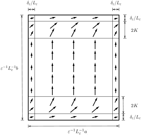
Figure 2: Schematics of the truncated test magnetization configuration $\widetilde{m}_{\delta_{\varepsilon}/L_{\varepsilon}}$ used in the upper bound construction of Sec. 6.

We now estimate the first intergal $I_{1}$. Using the definition of $\widetilde{\eta}_{\delta_{\varepsilon}/L_{\varepsilon}}$ we obtain that $\partial_{1}\widetilde{\eta}_{\delta_{\varepsilon}/L_{\varepsilon}}(x_{1},x_{2})=0$ for $\delta_{\varepsilon}L_{\varepsilon}^{-1}<x_{1}<\varepsilon^{-1}L_{\varepsilon}^{-1}b-\delta_{\varepsilon}L_{\varepsilon}^{-1}$. Moreover, outside this interval $|\partial_{1}\widetilde{\eta}_{\delta_{\varepsilon}/L_{\varepsilon}}(x_{1},x_{2})|\leq L_{\varepsilon}/\delta_{\varepsilon}$. We also know that $m_{\varepsilon,1}(x_{2})=0$ for $x_{2}\in(0,\delta_{\varepsilon}/L_{\varepsilon})\cup(2K+\delta_{\varepsilon}/L_{\varepsilon},\varepsilon^{-1}L_{\varepsilon}^{-1}b-2K-\delta_{\varepsilon}/L_{\varepsilon})\cup(\varepsilon^{-1}L_{\varepsilon}^{-1}b-\delta_{\varepsilon}/L_{\varepsilon})$, where $K$ is the same constant as in the one-dimensional construction. Therefore, by direct computation we can estimate for all $\varepsilon$ sufficiently small

$$I_{1}\leq C\left(\frac{L_{\varepsilon}}{\delta_{\varepsilon}}\right)^{2}\int_{0}^{2K+\delta_{\varepsilon}L_{\varepsilon}^{-1}}\int_{0}^{2K+\delta_{\varepsilon}L_{\varepsilon}^{-1}}\int_{0}^{\delta_{\varepsilon}L_{\varepsilon}^{-1}}\int_{0}^{\delta_{\varepsilon}L_{\varepsilon}^{-1}}{\,\mathrm{d}x_{1}\,\mathrm{d}\xi_{1}\,\mathrm{d}x_{2}\,\mathrm{d}\xi_{2}\over\sqrt{(x_{1}-\xi_{1})^{2}+(x_{2}-\xi_{2})^{2}}}\leq CK\ln\left(\frac{L_{\varepsilon}}{\delta_{\varepsilon}}\right),$$ (6.33)

for some universal $C>0$. Similarly, the last integral $I_{3}$ can be estimated as

$$I_{3}\leq C\left(\frac{L_{\varepsilon}}{\delta_{\varepsilon}}\right)\int_{\delta_{\varepsilon}L_{\varepsilon}^{-1}}^{2K+\delta_{\varepsilon}L_{\varepsilon}^{-1}}\int_{0}^{\varepsilon^{-1}L_{\varepsilon}^{-1}a}\int_{0}^{2K+\delta_{\varepsilon}L_{\varepsilon}^{-1}}\int_{0}^{\delta_{\varepsilon}L_{\varepsilon}^{-1}}\frac{\,\mathrm{d}x_{1}\,\mathrm{d}x_{2}\,\mathrm{d}\xi_{1}\,\mathrm{d}\xi_{2}}{\sqrt{(x_{1}-\xi_{1})^{2}+(x_{2}-\xi_{2})^{2}}}\\ +\left(\frac{L_{\varepsilon}}{\delta_{\varepsilon}}\right)^{2}\int_{0}^{\delta_{\varepsilon}L_{\varepsilon}^{-1}}\int_{0}^{\varepsilon^{-1}L_{\varepsilon}^{-1}a}\int_{0}^{2K+\delta_{\varepsilon}L_{\varepsilon}^{-1}}\int_{0}^{\delta_{\varepsilon}L_{\varepsilon}^{-1}}\frac{\,\mathrm{d}x_{1}\,\mathrm{d}x_{2}\,\mathrm{d}\xi_{1}\,\mathrm{d}\xi_{2}}{\sqrt{(x_{1}-\xi_{1})^{2}+(x_{2}-\xi_{2})^{2}}}\leq CK\ln\left(\frac{1}{\varepsilon}\right),$$ (6.34)

again, for some universal $C>0$ and all $\varepsilon$ small enough.

Proof of Theorem 3.4..

We can combine the lower bounds for $F_{\varepsilon}^{MM}$ and $F_{\varepsilon}^{S}$ and proceed in the same way as in the one-dimensional case. There is a slight mismatch, as the definition of $n_{\varepsilon}^{\pm}$ uses the average of $\widetilde{m}_{\delta_{\varepsilon}/L_{\varepsilon},2}$, while the lower bound (6.1) for $F_{\varepsilon}^{MM}$ uses $\overline{m}_{\varepsilon,2}$. However, we observe that

$$\left|\frac{\varepsilon L_{\varepsilon}}{a}\int_{0}^{\varepsilon^{-1}L_{\varepsilon}^{-1}a}\widetilde{m}_{\delta_{\varepsilon}/L_{\varepsilon},2}(x_{1},x_{2})\,\mathrm{d}x_{1}-\overline{m}_{\varepsilon,2}(x_{2})\right|\\ \leq\frac{\varepsilon L_{\varepsilon}}{a}\int_{0}^{\varepsilon^{-1}L_{\varepsilon}^{-1}a}|m_{\varepsilon,2}(x_{1},x_{2})|(1-\tilde{\eta}_{\delta_{\varepsilon}/L_{\varepsilon}}(x_{1},x_{2}))\,\,\mathrm{d}x_{1}\leq C\varepsilon\delta_{\varepsilon},$$ (6.35)

for some $C>0$ independent of $\varepsilon$, and, therefore, asymptotically we can interchange the average of $\widetilde{m}_{\delta_{\varepsilon}/L_{\varepsilon},2}$ with $\overline{m}_{\varepsilon,2}$ in the formula in (6.1) and arrive at the full lower bound as in the one-dimensional case. Using in addition the upper bound construction, the proof of (3.17) follows exactly as in the proof of Theorem 3.2 with the help of Lemma 6.1. Convergence of $m_{\varepsilon}$ to $e_{2}$ trivially follows from positivity of the stray field energy and boundedness of $E_{\varepsilon}(m_{\varepsilon})$ as $\varepsilon\to 0$.

Assuming $m_{\varepsilon}$ is a minimizer of $E_{\varepsilon}$, in the same way as in the proof of the Theorem 3.2 it follows that $n_{\varepsilon}^{-}\to n_{0}$ and $n_{\varepsilon}^{+}\to n_{0}$, therefore we have

$$\overline{m}_{\delta_{\varepsilon}/L_{\varepsilon},2}({\delta_{\varepsilon}}/{L_{\varepsilon}})\to n_{0}\quad\hbox{ and }\quad\overline{m}_{\delta_{\varepsilon}/L_{\varepsilon},2}({b}/({\varepsilon L_{\varepsilon}})-{\delta_{\varepsilon}}/{L_{\varepsilon}})\to n_{0}.$$ (6.36)

Using the inequality in (6.35) and recalling (6.4), we obtain the desired result. ∎

References

- [1] S. D. Bader and S. S. P. Parkin. Spintronics. Ann. Rev. Cond. Mat. Phys., 1:71–88, 2010.
- [2] F. Bethuel and X. M. Zheng. Density of smooth functions between two manifolds in Sobolev spaces. J. Funct. Anal., 80:60–75, 1988.
- [3] J. Bourgain, H. Brezis, and P. Mironescu. Lifting in Sobolev spaces. J. Anal. Math., 80:37–86, 2000.
- [4] A. Brataas, A. D. Kent, and H. Ohno. Current-induced torques in magnetic materials. Nature Mat., 11:372–381, 2012.
- [5] H. Brezis. Functional Analysis, Sobolev Spaces and Partial Differential Equations. Springer, 2011.
- [6] W. F. Brown. Micromagnetics. Interscience Tracts of Physics and Astronomy 18. Interscience Publishers (Wiley & Sons), 1963.
- [7] A. Capella, C. Melcher, and F. Otto. Wave-type dynamics in ferromagnetic thin films and the motion of Néel walls. Nonlinearity, 20:2519—2537, 2007.
- [8] M. Chermisi and C. B. Muratov. One-dimensional Néel walls under applied external fields. Nonlinearity, 26:2935–2950, 2013.
- [9] H. S. Cho, C. Hou, M. Sun, and H. Fujiwara. Characteristics of 360∘-domain walls observed by magnetic force microscope in exchange-biased NiFe films. J. Appl. Phys., 85:5160–5162, 1999.
- [10] C. L. Dennis, R. P. Borges, L. D. Buda, U. Ebels, J. F. Gregg, M. Hehn, E. Jouguelet, K. Ounadjela, I. Petej, I. L. Prejbeanu, and M. J. Thornton. The defining length scales of mesomagnetism: A review. J. Phys. – Condensed Matter, 14:R1175–R1262, 2002.
- [11] A. DeSimone, R. V. Kohn, S. Müller, and F. Otto. Magnetic microstructures—a paradigm of multiscale problems. In ICIAM 99 (Edinburgh), pages 175–190. Oxford Univ. Press, 2000.
- [12] A. DeSimone, R. V. Kohn, S. Müller, and F. Otto. Recent analytical developments in micromagnetics. In G. Bertotti and I. D. Mayergoyz, editors, The Science of Hysteresis, volume 2 of Physical Modelling, Micromagnetics, and Magnetization Dynamics, pages 269–381. Academic Press, Oxford, 2006.
- [13] E. Di Nezza, G. Palatucci, and E. Valdinoci. Hitchhiker’s guide to the fractional Sobolev spaces. Bull. Sci. Math., 136:521–573, 2012.
- [14] W. E, W. Ren, and E. Vanden-Eijnden. Energy landscape and thermally activated switching of submicron-sized ferromagnetic elements. J. Appl. Phys., 93:2275–2282, 2003.
- [15] J. Fidler and T. Schrefl. Micromagnetic modelling—the current state of the art. J. Phys. D: Appl. Phys., 33:R135–R156, 2000.
- [16] C. J. Garcia-Cervera and W. E. Effective dynamics for ferromagnetic thin films. J. Appl. Phys., 90:370–374, 2001.
- [17] F. Hellman et al. Interface-induced phenomena in magnetism. Rev. Mod. Phys., 89:025006, 2017.
- [18] S. Hirono, K. Nonaka, and I. Hatakeyama. Magnetization distribution analysis in the film edge region under a homogeneous field. J. Appl. Phys., 60:3661–3670, 1986.
- [19] R. M. Hornreich. 90 magnetization curling in thin films. J. Appl. Phys., 34:1071–1072, 1963.
- [20] R. M. Hornreich. Magnetization curling in tapered edge films. J. Appl. Phys., 35:816–817, 1964.
- [21] A. Hubert and R. Schäfer. Magnetic Domains. Springer, Berlin, 1998.
- [22] H. Knüpfer, C. B. Muratov, and F. Nolte. Magnetic domains in thin ferromagnetic films with strong perpendicular anisotropy. Preprint: arXiv:1702.01980, 2017.
- [23] R. V. Kohn and V. V. Slastikov. Another thin-film limit of micromagnetics. Arch. Ration. Mech. Anal., 178:227–245, 2005.
- [24] R. V. Kohn and V.V. Slastikov. Effective dynamics for ferromagnetic thin films: a rigorous justification. Proc. R. Soc. Lond. Ser. A, 461:143–154, 2005.
- [25] M. Kurzke. Boundary vortices in thin magnetic films. Calc. Var. Partial Differential Equations, 26:1–28, 2006.
- [26] E. H. Lieb and M. Loss. Analysis. American Mathematical Society, Providence, RI, 2010.
- [27] R. G. Lund, C. B. Muratov, and V. V. Slastikov. One-dimensional in-plane edge domain walls in ultrathin ferromagnetic films. Nonlinearity, 31:728–754, 2018.
- [28] R. Mattheis, K. Ramstöck, and J. McCord. Formation and annihilation of edge walls in thin-film permalloy strips. IEEE Trans. Magn., 33:3993–3995, 1997.
- [29] V. Milisic and U. Razafison. Weighted Sobolev spaces for the Laplace equation in periodic infinite strips. arXiv:1302.4253, 2013.
- [30] L. Modica. The gradient theory of phase transitions and the minimal interface criterion. Arch. Rational Mech. Anal., 98:123–142, 1987.
- [31] R. Moser. Boundary vortices for thin ferromagnetic films. Arch. Ration. Mech. Anal., 174:267–300, 2004.
- [32] C. B. Muratov. A universal thin film model for Ginzburg-Landau energy with dipolar interaction. Preprint: arXiv:1702.01986, 2017.
- [33] C. B. Muratov and V. V. Osipov. Optimal grid-based methods for thin film micromagnetics simulations. J. Comp. Phys., 216:637–653, 2006.
- [34] C. B. Muratov and V. V. Osipov. Theory of domain walls in thin ferromagnetic films. J. Appl. Phys., 104:053908 pp. 1–14, 2008.
- [35] C. B. Muratov and V. V. Slastikov. Domain structure of ultrathin ferromagnetic elements in the presence of Dzyaloshinskii-Moriya interaction. Proc. R. Soc. Lond. Ser. A, 473:20160666, 2016.
- [36] J. Nogues, J. Sort, V. Langlais, V. Skumryev, S. Surinach, J. S. Munoz, and M. D. Baro. Exchange bias in nanostructures. Phys. Rep., 422:65–117, 2005.
- [37] K. Nonaka, S. Hirono, and I. Hatakeyama. Magnetostatic energy of magnetic thin-film edge having volume and surface charges. J. Appl. Phys., 58:1610–1614, 1985.
- [38] C. Ortner and E. Süli. A note on linear elliptic systems on . arXiv:1202.3970v3, 2012.
- [39] G. A. Prinz. Magnetoelectronics. Science, 282:1660–1663, 1998.
- [40] G. O. G. Rebouças, A. S. W. T. Silva, Ana L. Dantas, R. E. Camley, and A. S. Carriço. Magnetic hysteresis of interface-biased flat iron dots. Phys. Rev. B, 79:104402, 2009.
- [41] M. Rührig, W. Rave, and A. Hubert. Investigation of micromagnetic edge structures of double-layer permalloy films. J. Magn. Magn. Mater., 84:102–108, 1990.
- [42] V. V. Slastikov. Micromagnetics of thin shells. Math. Models Methods Appl. Sci., 15:1469–1487, 2005.
- [43] A. Soumyanarayanan, N. Reyren, A. Fert, and C. Panagopoulos. Emergent phenomena induced by spin–orbit coupling at surfaces and interfaces. Nature, 539:509–517, 2016.
- [44] R. H. Wade. Some factors in easy axis magnetization of permalloy films. Phil. Mag., 10:49–66, 1964.