Fundraising and vote distribution: a non-equilibrium statistical approach

Abstract

The number of votes correlates strongly with the money spent in a campaign, but the relation between the two is not straightforward. Among other factors, the output of a ballot depends on the number of candidates, voters, and available resources. Here, we develop a conceptual framework based on Shannon entropy maximization and Superstatistics to establish a relation between the distributions of money spent by candidates and their votes. By establishing such a relation, we provide a tool to predict the outcome of a ballot and to alert for possible misconduct either in the report of fundraising and spending of campaigns or on vote counting. As an example, we consider real data from a proportional election with $6323$ candidates, where a detailed data verification is virtually impossible, and show that the number of potential misconducting candidates to audit can be reduced to only nine.

In an effort towards fair electoral processes, regulations and reforms are constantly on the agenda of many countries around the world Secretary General (2009). To avoid that the decision-making process is dominated by wealth and influence, the most pertinent processes to legislate are arguably fundraising and spending for Democracy and Assistance (2002). Different countries have different rules, but in general, candidates and parties are the ones that report on the financial details of their own campaigns, what raises obvious doubts over the veracity of the reported data. As the number of collected votes correlates with the money spent in the campaign Melo et al. (2018), establishing a quantitative relation between the distribution of votes and financial resources among the candidates is instrumental to raise flags about possible misconduct.

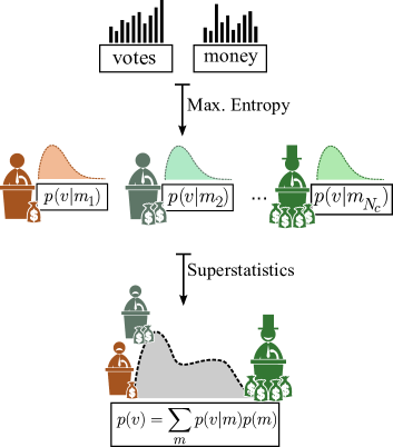
Figure 1: By employing the principle of maximum entropy under the constraints of a fixed number of voters and candidates, we derive the conditional probability $p(v|m_{i})$, that a candidate $i$ receives $v$ votes, provided that $i$ spends an amount of money $m_{i}$ in the campaign. Since the amount of money spent usually differ from candidate to candidate, the final distribution of votes should depend on the distribution of money spent. A formalism based on Superstatistics Beck and Cohen (2003) is then used to establish a relation between these two distributions. 

Within some regulated boundaries, several individuals or institutions can contribute financially to a campaign. The value of the contribution is very subjective, depending on their interests and on the economic and political conjecture Jacobson (1978); Morton and Cameron (1992); Gerber (2004); Gordon et al. (2007). Thus, predicting the distribution of funds raised and money spent in a campaign from “first principles” is likely a hopeless endeavor, challenging the verification of the reported data. In sharp contrast, the distribution of votes among candidates is well studied. It is known to differ for proportional and plural elections, and to depend on the country, number of candidates, and money spent in campaigns Costa Filho et al. (1999, 2003); Castellano et al. (2009); Mantovani et al. (2011, 2013); Bokányi et al. (2018). Different models were developed to explain this distribution Melo et al. (2018); Moreira et al. (2006); Araújo et al. (2010); Fernández-Gracia et al. (2014); Calvão et al. (2015); Borghesi et al. (2012); Fortunato and Castellano (2007) as well as methodologies to identify vote-counting irregularities Lehoucq (2003); Alvarez et al. (2009); Deckert et al. (2011); Klimek et al. (2012); Beber and Scacco (2012); Enikolopov et al. (2013). Here we propose an approach based on the Shannon entropy maximization and Superstatistics to disclose a relation between the distribution of financial resources declared by candidates and the distribution of their votes in proportional elections.

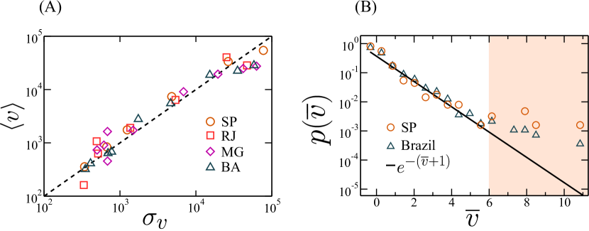
Figure 2: Empirical data for the 2014 election for federal deputies in Brazil, which counted $6323$ candidates, roughly $140$ million voters, and more than $280$ million dollars of total investment in campaigns. (A) The average number as a function of the standard deviation of votes per candidate at the state level, for the top four populated Brazilian states, namely, São Paulo (SP, circles), Rio de Janeiro (RJ, squares), Minas Gerais (MG, diamonds), and Bahia (BA, triangles). For each state, candidates were grouped by the amount of money that they officially declared to have spent in their campaigns. The dashed line corresponds to a linear behavior. (B) Distribution of rescaled number of votes $\bar{v}=(v-\langle v\rangle)/\sigma_{v}$ for São Paulo (blue triangles) and the entire country of Brazil (black circles), where $\langle v\rangle$ and $\sigma_{v}$ are the average and standard deviation of the number of votes received by the candidates in the same interval (logarithmic binning) of money spent. The (red)-dashed line corresponds to $p(v)=\exp(-\bar{v}-1)$, as predicted by Eq. (5), if we assume $Z(m)=\mu$. Following the prediction given by Eq. (5) from our theoretical approach, the distribution of votes for more than $99\%$ of the candidates follows an exponential distribution. However, it is remarkable that the number of candidates with votes that deviate more than $6\sigma_{v}$ (highlighted region) from the average is higher than expected, suggesting the existence of outliers. 

Given a certain amount of money $m_{i}$ spent by a candidate $i$ in the campaign, the conditional probability for $i$ to receive $v$ votes is $p(v|m_{i})$. Since the money spent is heterogeneously distributed among candidates, the probability $p(v)$ that a candidate receives $v$ votes is given by,

$$p(v)=\sum_{m=0}^{m_{\mathrm{max}}}p(v|m)p(m)\ \ ,$$ (1)

where $p(m)$ is the probability that a candidate spends an amount of money $m$ in the campaign and $m_{\mathrm{max}}$ is the maximum amount of money that can be spent (see Fig. 1). For simplicity, we have considered that $m$ is a discrete variable and a multiple of $\Delta m$, where $\Delta m$ is the “price of a vote”. Equation (1) is the basis of Superstatistics for non-equilibrium systems Beck and Cohen (2003), a theoretical framework developed to describe the thermal fluctuations of an ensemble of particles at different effective thermostat temperatures and consequently different weights for each configuration. Analogously, in an election, the amount of money spent differs from candidate to candidate and thus also the probability that they receive a certain number of votes. As a consequence, the variable $m$ is the analogue for elections of the thermostat temperature in a thermal system.

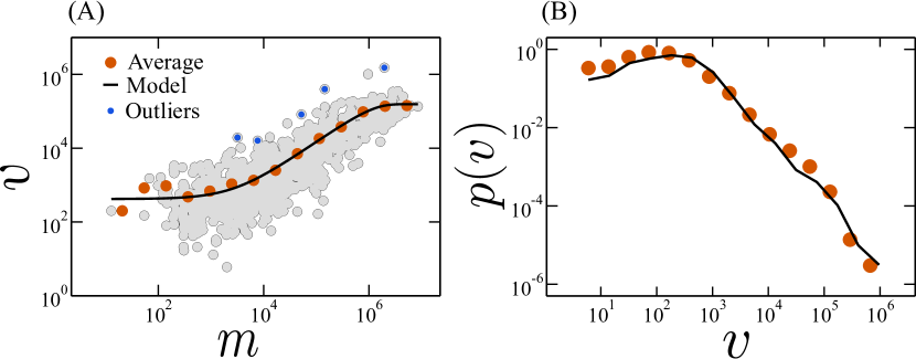
Figure 3: Results for the 2014 election for federal deputies in the state of São Paulo, Brazil, with $1364$ candidates, more than $32$ million voters, and about $58$ million dollars of total investment in the campaigns. (A) Number of votes as a function of the money spent in the campaign for all candidates (gray dots) and the average value within each money group (blue-dark dots). The (red-)solid line is obtained by a least-squares fit of Eq. (7) to the average data, taking $\Delta m$ as a free parameter. The black circles are outliers, which we defined as the candidates with a number of votes that deviate more than $6\sigma_{v}$ from the average. (B) Distribution of the number of votes per candidate. The (red) dots were obtained from the data and the solid line was calculated from the distribution of money spent in the campaign. Precisely, the solid line is obtained by randomly assigning a number of votes $v$ for each candidate from the distribution given by Eq. (5), where $m$ is the amount of money officially declared to have been spent in the campaign. The obtained curve is remarkably consistent with the empirical data over more than five orders of magnitude. 

To calculate $p(v|m)$, let us consider a proportional election with $N_{c}$ candidates and $N_{v}$ voters. Based on the principle of maximum entropy Jaynes (1957), $p(v|m)$ should maximize the Shannon entropy,

$$S=-\sum_{i=1}^{N_{c}}\sum_{v=v_{0}}^{m_{i}/\Delta m}p(v|m_{i})\ln[p(v|m)]\ \ ,$$ (2)

where $v_{0}$ and $m_{i}/\Delta m$ are the minimum and maximum number of votes that the candidate $i$ can receive. For simplicity, hereafter we assume that $v_{0}$ is the same for all candidates. At this point, two constraints need to be imposed, as both the number of candidates $N_{c}$ and voters $N_{v}$ are fixed (see Fig. 1). In this way, the first constraint is then,

$$\sum_{i=0}^{N_{c}}\sum_{v=v_{0}}^{m_{i}/\Delta m}p(v|m_{i})=N_{c}\ \ ,$$ (3)

which ensures the normalization of $p(v|m)$, while the second one is,

$$\sum_{i=0}^{N_{c}}\sum_{v=v_{0}}^{m_{i}/\Delta m}vp(v|m_{i})=N_{v}\ \ .$$ (4)

By maximizing $S$ subjected to Eqs. (3) and (4), we obtain

$$p(v|m)=\frac{1}{Z(m)}e^{-\mu v}\ \ ,$$ (5)

where $Z(m)$ is a normalization factor that depends on $m$ and it is the analogue of the partition function in a thermal system, given by,

$$Z(m)=\frac{e^{\mu(1-v_{0})}-e^{-\mu m/\Delta m}}{e^{\mu}-1}\ \ ,$$ (6)

where $\mu$ is the Lagrange multiplier related to the second constraint (Eq. (4)). Since the number of votes is limited, $p(v|m)$ decays exponentially for $v\in[v_{0},m/\Delta m]$ and it is zero otherwise.

In order to verify if the distribution predicted by Eq. (5) is compatible with real data, we consider the 2014 election for federal deputies in Brazil, using the dataset available in Ref. dat . Each state has its own ballot, with different candidates and voters. Countrywide, this is an election with $6323$ candidates, roughly $140$ million voters, and more than $280$ million dollars invested in campaigns. We first analyze the results for the top four populated Brazilian states, namely, São Paulo, Rio de Janeiro, Minas Gerais, and Bahia. These states have each more than $10$ million voters and between $239$ (Bahia) and $1364$ (São Paulo) candidates. For each state, we grouped the candidates by the amount of money that they reported to have spent in their campaigns. Figure 2A shows the average number of votes $\langle v\rangle$ received by a candidate as a function of the standard deviation $\sigma_{v}$ for each money group. For most data point, the results are consistent with a linear behavior (dashed line) as expected for an exponential distribution, where the average and standard deviation are always equal. To verify the functional dependence of the distribution, in Fig. 2B shows the distribution of votes, rescaled as $\bar{v}=(v-\langle v\rangle)/\sigma_{v}$, where $\langle v\rangle$ and $\sigma_{v}$ is the average and standard deviation of the number of votes per candidate in the same interval (logarithmic binning) of money spent. The distribution clearly follows the predicted exponential behavior of Eq. (5) for more than $99\%$ of the candidates. However, for $\bar{v}>6$ the distribution deviates from the predicted one (highlighted region in Fig. 2B). There are nine candidates in this region in the entire country, with five of them running in São Paulo. This is remarkable, as the theory predicts five in the entire country and only one in São Paulo. This observation raises doubts about these outliers and it could therefore call for a detailed analysis and validation of their reported data about the campaign founding.

From the partition function (6), the average number of votes received by a candidate that spent $m$ money in the campaign is,

$$\langle v\rangle=v_{0}+\frac{1}{e^{\mu}-1}+\frac{1-v_{0}+m/\Delta m}{1-e^{\mu(1-v_{0}+m/\Delta m)}}\ \ .$$ (7)

The value of $\mu$ is obtained by imposing the second constraint (Eq. (4)) and considering $\Delta m$ as a free parameter. Figure 3A shows the number of votes per candidate against the money spent in the campaign (gray circles) and the average value for candidates in the same money group (orange circles), where the circles in blue correspond to the outliers. The solid line in Fig. 3A is the non-linear fit of Eq. 7 to the numbers of votes of all candidates as a function of their financial resources, which gives $\Delta m=2.07$. As shown, the excellent agreement between this fit and the averaged data points extends over four orders of magnitude, with deviations found only for candidates with very scarce resources, a fact that can be explained as follows. For simplicity, we have considered that the minimum number of votes $v_{0}$ is the same for all candidates, obtained by assuming that $v_{0}$ equals the average number of votes for candidates who spent less than $1200$ dollars Melo et al. (2018). In general, however, every candidate has a different $v_{0}$, depending on several factors such as, his/her party, visibility, and social status.

Through Eq. (5), it is also possible to predict, from the reported amount of money spent by each campaign, the distribution of votes for an election. As an example, let us consider again the election in the state of São Paulo. Figure 3B shows the distribution of the number of votes (red dots) obtained by each candidate. To predict the distribution of votes for this election, we assigned randomly a number of votes to each candidate from a distribution given by Eq. (5), with $m$ equal to the amount of money spent in the campaign, as declared by the candidate. The solid line in Fig. 3B is the predicted outcome, which is in excellent agreement with the empirical data. Once more, in the proposed framework, $\Delta m$ is a free parameter that relates to the amount of money spent by a candidate campaign and the maximum number of votes that it can receive. Its value was estimated by fitting Eq. (7), as explained before.

Conclusions. We have shown, using the principle of maximum entropy, that the distribution of votes received by a candidate should follow an exponential distribution parameterized by the amount of money that was spent in her/his campaign. This prediction is consistent with real data from a very large proportional election, with $6323$ candidates. Furthermore, as the money spent in a campaign is heterogeneously distributed among candidates, we developed a framework based on superstatistics to establish the relation between the distribution of money spent and of votes. Within this framework, it was possible to predict the outcome of a ballot from the distribution of money spent, and identify potential cases of misconduct either in the report of fundraising and spending or on vote counting.

For several proportional elections, the distribution of votes per candidate is fat tailed Chatterjee et al. (2013), what has motivated an enthusiastic discussion about the underlying mechanism Castellano et al. (2009). As our theoretical approach shows, for an election, if all candidates spent the same amount of money in their campaigns, the expected distribution of votes would be exponential. So, the fat-tailed distribution is a consequence of an heterogeneous distribution of resources. This is consistent with the reported power-law distribution of money spent by candidates in the same elections Melo et al. (2018).