An FE-dABCD algorithm for elliptic optimal control problems with constraints on the gradient of the state and control.

Abstract

In this paper, elliptic control problems with integral constraint on the gradient of the state and box constraints on the control are considered. The optimal conditions of the problem are proved. To numerically solve the problem, we use the First discretize, then optimize approach. Specifically, we discretize both the state and the control by piecewise linear functions. To solve the discretized problem efficiently, we first transform it into a multi-block unconstrained convex optimization problem via its dual, then we extend the inexact majorized accelerating block coordinate descent (imABCD) algorithm to solve it. The entire algorithm framework is called finite element duality-based inexact majorized accelerating block coordinate descent (FE-dABCD) algorithm. Thanks to the inexactness of the FE-dABCD algorithm, each subproblems are allowed to be solved inexactly. For the smooth subproblem, we use the generalized minimal residual (GMRES) method with preconditioner to slove it. For the nonsmooth subproblems, one of them has a closed form solution through introducing appropriate proximal term, another is solved combining semi-smooth Newton (SSN) method. Based on these efficient strategies, we prove that our proposed FE-dABCD algorithm enjoys $O(\frac{1}{k^{2}})$ iteration complexity. Some numerical experiments are done and the numerical results show the efficiency of the FE-dABCD algorithm.

1 Introduction

Optimal control problems with constraints on the gradient of the state have a wide range of important applications. For instance, in cooling processes or structured optimization when high stresses have to be avoided. In cooling processes, constraints on the gradient of the state play an important role in practical applications where solidification of melts forms a critical process. In order to accelerate the production, it is highly desirable to speed up the cooling processes while avoiding damage of the products caused by large material stresses. Cooling frequently is described by systems of partial differential equations involving the temperature as a system variable, so that large (Von Mises) stresses in the optimization can be kept small by imposing bounds on the gradient of the temperature (see Wollner2013A ; Nther2011Elliptic ).

Optimal control problems with constraints on the gradient of the state have caused much attention. For optimal control problems with pointwise constraints on the gradient of the state, there are some existing works on the optimal conditions Casas1993Optimal , discretization Deckelnick2014A and error analysis Wollner2013A ; Nther2011Elliptic ; Deckelnick2014A . Since the Lagrange multiplier corresponding to the pointwise constraint on the gradient of the state in general only represents a regular Borel measure (see Casas1993Optimal ), the complementarity condition in the optimal conditions cannot be written into a pointwise form, which brings some difficulties and reduces flexibility of the numerical realization. As we know, although this difficulty can be solved by some common regularization approaches such as Lavrentiev regularization Meyer2006Optimal ; Pr2007On ; Chen2016A and Moreau-Yosida regularization hintermuller2006feasible ; hintermuller2006path ; Itoa2003Semi ; Kunisch2010Optimal , the efficiency of these regularization approaches usually depends on the choice of the regularization parameters, which will also bring some difficulties. To relax the pointwise constraint, in this paper, as a model problem we consider the following elliptic PDE-constrained optimal control problem with box constraints on the control and integral constraint on the gradient of state.

$$\qquad\left\{\begin{aligned} \min\limits_{(y,u)\in Y\times U}\ \ J(y,u)&=\frac{1}{2}\|y-y_{d}\|_{L^{2}(\mathrm{\Omega})}^{2}+\frac{\alpha}{2}\|u\|_{L^{2}(\mathrm{\Omega})}^{2}\\ {\mathrm{s.t.}}\qquad\quad\ \ \mathcal{A}y&=u+f\quad\mathrm{in}\ \mathrm{\Omega},\\ y&=0\qquad\quad\mathrm{on}\ \mathrm{\Gamma},\\ \nabla y&\in\mathcal{K},\\ u&\in\mathcal{W},\end{aligned}\right. \mathrm{P}$$ ()

where $Y:=H_{0}^{1}(\mathrm{\Omega})$, $U:=L^{2}(\mathrm{\Omega})$, $\mathrm{\Omega}\subseteq\mathbb{R}^{n}\ (n=2,3)$ is a convex, open and bounded domain with $C^{1,1}$- or polygonal boundary $\mathrm{\Gamma}$; the desired state $y_{d}\in L^{2}(\mathrm{\Omega})$ and $f\in L^{2}(\mathrm{\Omega})$ are given; $a,\ b\in\mathbb{R}$ and $\alpha>0$ are given parameters; $\mathcal{K}=\{\mathbf{z}\in{L^{2}(\bar{\mathrm{\Omega}})}^{n}|\int_{\mathrm{\Omega}}|\mathbf{z}(x)|^{2}dx\leq\delta\}$ is a closed convex subset of ${L^{2}(\mathrm{\Omega})}^{n}$ with nonempty interior, $\mathcal{W}=\{v\in L^{\infty}(\mathrm{\Omega})|\ a\leq v\leq b\quad\mathrm{a.e.}\ x\in\mathrm{\Omega}\}$ is a nonempty convex closed subset of $U$; $\mathcal{A}$ is a uniformly elliptic operator

$$(\mathcal{A}y)(x):=-\sum^{n}_{i,j=1}\partial_{x_{j}}(a_{ij}y_{x_{i}})+c_{0}y,$$ (1)

where $a_{ij}$, $c_{0}\in L^{\infty}(\mathrm{\Omega})$, $c_{0}\geq 0$, $a_{ij}=a_{ji}$ and there is a constant $\theta>0$ such that

$$\sum_{i,j=1}^{n}a_{ij}(x)\xi_{i}\xi_{j}\geq\theta\|\xi\|^{2}\quad\mathrm{for\ a.a.}\ x\in\mathrm{\Omega}\ \mathrm{and}\ \xi\in\mathbb{R}^{n}.$$

We use $|\cdot|$ to denote the Euclidean norm, use ${\rm{(\cdot,\cdot)}}$ to denote the inner product in $L^{2}(\mathrm{\Omega})$ and use $\|\cdot\|$ to denote the corresponding norm.

Remark 1

Although we assume that the operator $\mathcal{A}$ is a uniformly elliptic operator and Dirichlet boundary condition $y=0$ holds, we would like to point out that our considerations can also carry over to parabolic operators and more general boundary conditions of Robin type

$$\partial_{n}y+\gamma y=g\qquad\mathrm{on}\ \mathrm{\Gamma},$$

where $g\in L^{2}(\mathrm{\Gamma})$ is given and $\gamma\in L^{\infty}(\mathrm{\Gamma})$ is a nonnegative coefficient.

To numerically solve problem ($\mathrm{P}$), there are two possible ways. One is called First discretize, then optimize, another is called First optimize, then discretize Collis2002Analysis . Independently of where discretization is located, the resulting finite dimensional equations are quite large. Hence, both cases require us to consider proposing an efficient algorithm based on the structure of the problem. In this paper, we use the First discretize, then optimize approach. With respect to the discrete methods, we use the full discretization method, in which both the state and control are discretized by piecewise linear functions.

As we know, there are many first order algorithms being used to solve finite dimensional large scale optimization fast, such as iterative soft thresholding algorithms (ISTA) Blumensath2008Iterative , fast iterative soft thresholding algorithms (FISTA) Beck2009A , accelerated proximal gradient (APG)-based method jiang2012inexact ; toh2010accelerated and alternating direction method of multipliers (ADMM) li2015qsdpnal ; li2016schur ; Chen2016A . Motivated by the success of these first order algorithms, an APG method in function space (called Fast Inexact Proximal (FIP) method) was proposed to solve the elliptic optimal control problem involving $L^{1}$-control cost in schindele2016proximal . It is known that whether the APG method is efficient depends closely on whether the step-length is close enough to the Lipschitz constant, however, the Lipschitz constant is not easy to estimate in usual, which largely limits the efficiency of APG method. Recently, an inexact heterogeneous ADMM (ihADMM) algorithm was proposed and used to solve optimal control problems with $L^{1}$-control cost in Song2017A . Simultaneously, the authors also extended it to optimal control problems with $L^{2}$-control cost in Song2016A and Lavrentiev-regularized state-constrained optimal control problem in Chen2016A . It is known that its iteration scheme is simple and each subproblem can be solved efficiently. However, ihADMM algorithm only has $O(\frac{1}{k})$ iteration complexity.

Most of the papers mentioned above are devoted to solving the primal problem. However, Song et al. Song2018An proposed an duality-based approach for PDE-constrained sparse optimization, which reformulated the problem as a multi-block unconstrained convex composite minimization problem and proposed a sGS-imABCD algorithm to solve the problem. Motivated by it, we consider solving ($\mathrm{P}$) via its dual. We find that we can also reformulate our problem as a multi-block unconstrained convex optimization problem and take advantage of the structure of it to construct an efficient algorithm to solve it efficiently and fast. Specifically, it is shown in Section 4.1 that the dual problem of discretization version of ($\mathrm{P}$) can be written as

$$\min\limits_{p,\lambda,\mu}\ F(p,\lambda,\mu)= \frac{1}{2}\|{K_{h}}^{T}p+\lambda-M_{h}y_{d}\|_{{M_{h}^{-1}}}^{2}+\frac{1}{2\alpha}\|M_{h}p-\mu\|_{{M_{h}^{-1}}}^{2}$$ (2)

$$+\delta^{*}_{\mathcal{C}}(\lambda)+\delta^{*}_{\mathcal{S}}(\mu)+(M_{h}f,p)-\frac{1}{2}\|y_{d}\|_{M_{h}}^{2},$$

where $p$, $\lambda$, $\mu\in{\mathbb{R}}^{n}$ and for any given nonempty, closed convex subset $B$ of ${\mathbb{R}}^{n}$, $\delta_{B}(\cdot)$ denotes the indicator function of $B$. That is to say

$$\delta_{B}(x)=\left\{\begin{aligned} &1,\qquad&x\in B,\\ &\infty,&x\notin B.\end{aligned}\right.$$ (3)

Based on inner product, the conjugate of $\delta_{B}(\cdot)$ is defined as follows

$$\delta_{B}^{*}(y) =\sup_{x}\ \{(y,x)-\delta_{B}(x)\},$$ (4)

$$=\sup_{x\in B}\ (y,x).$$

It is easy to see that (2) is a multi-block unconstrained minimization problem including two non-smooth terms, which are decoupled. In this case, block coordinate descent (BCD) method (see Grippo2000On ; Sardy2000Block ; Tseng1993Dual ; Tseng2001Convergence ) is top-priority and appropriate. Combining BCD method and the acceleration technique in APG will result in accelerated block coordinate descent (ABCD) method. It is a natural idea that we use ABCD method to solve (2), however, the convergence property of $3$ block ABCD method can not be promised (see Chambolle2015A ). Fortunately, in our problem, $\lambda$ and $\mu$ can be seen as one block because of the important fact that $\lambda$ and $\mu$ are decoupled. Then (2) can be seen as an unconstrained convex optimization problem with coupled objective functions of the following form

$$\min_{v,w}\ f(v)+g(w)+\phi(v,w).$$ (5)

For unconstrained convex optimization problems with coupled objective functions of form (5), an accelerated alternative descent (AAD) algorithm was proposed in Chambolle2015A to solve it for the situation that the joint objective function $\phi$ is quadratic. However, the AAD method does not take the inexactness of the solutions of the associated subproblems into account. It is known that, in some case, exactly computing the solution of each subproblem is either impossible or extremely expensive. Sun et al. Sun2015An proposed an inexact accelerated block descent (iABCD) method to solve least squares semidefinite programming (LSSDP) via its dual, whose basic idea is first reducing the two block nonsmooth terms into one through applying the Danskin-type theorem and then using APG method to solve the reduced problem. However, for the situation that the subproblem with respect to $w$ could not be solved exactly, Danskin-type theorem can no longer be used to reduce two block nonsmooth terms into one.

To overcome the bottlenecks above, an inexact majorized accelerated block coordinate descent (imABCD) method was proposed in (cui2016, , Chapter 3). Under suitable assumptions and certain inexactness criteria, the author proved that the imABCD method enjoys $O(\frac{1}{k^{2}})$ iteration complexity. Motivated by its success, in this paper, we propose a finite element duality-based inexact majorized accelerating block coordinate descent (FE-dABCD) algorithm. One distinctive feature of our proposed method is that it employs a majorization technique, which gives us a lot of freedoms to flexibly choose different proximal terms for different subproblems. Moreover, thanks to the inexactness of our proposed method, we have the essential flexibility that the inner subproblems are allowed to be solved only approximately. We would like to emphasize that these flexibilities are essential. First, the flexibility of choosing proximal terms makes each problem maintain good structure and can be solved efficiently. In addition, with some simple and implementable error tolerance criteria, the cost for inexactly solving the subproblems can be greatly reduced, which further contributes to the efficiency of the proposed method. Specifically, we can see from the content in Section 4.3 that the smooth subproblem, i.e. $p$-subproblem, is a $2*2$ block saddle point system, which can be solved efficiently by some Krylov-based methods with preconditioner, such as the generalized minimal residual (GMRES) method with preconditioner. As for the nonsmooth subproblems, i.e. subproblems with regard to $\lambda$ and $\mu$, the $\lambda$-subproblem has a closed form solution through introducing an appropriate proximal term and the $\mu$-subproblem is solved by combining semi-smooth Newton (SSN) method efficiently. Moreover, the $O(\frac{1}{k^{2}})$ iteration complexity of the FE-dABCD algorithm is also proved.

The rest of this article is structured as follows. In Section 2, we will discuss the optimal conditions of problem ($\mathrm{P}$). Then we will consider its discretization in Section 3. Section 4 will give a duality-based approach to transform the discretized problem into a multi-block unconstrained convex optimization problem. Then a brief sketch of the imABCD method will be given and our proposed FE-dABCD algorithm will be described in details. Some numerical experiments will be given in Section 5 to verify the efficiency of the proposed algorithm. Finally, we will make a simple summary in Section 6.

2 Optimal Conditions

For the existence and uniqueness of the solution of the PDE equation in problem ($\mathrm{P}$)

$$\left\{\begin{aligned} \mathcal{A}y&=u+f\quad\mathrm{in}\ \mathrm{\Omega},\\ y&=0\qquad\quad\mathrm{on}\ \mathrm{\Gamma},\end{aligned}\right.$$ (6)

where $\mathcal{A}$ is defined by (1), the following theorem holds.

Theorem 2.1

(Hinze2009Optimization, , Theorem 1.23) For each $u\in L^{2}(\mathrm{\Omega})$, there exists a unique weak solution $y_{u}\in H^{1}_{0}(\mathrm{\Omega})$ of (6) and satifies

$$\|y_{u}\|_{H^{1}(\mathrm{\Omega})}\leq C_{1}(\|u\|_{L^{2}(\mathrm{\Omega})}+\|f\|_{L^{2}(\mathrm{\Omega})}),$$

where $C_{1}$ depends only on $a_{ij}$, $c_{0}$, $\mathrm{\Omega}$.

The weak formulation of (6) is given by

$${\rm{Find}}\ y\in H^{1}_{0}(\mathrm{\Omega}):\quad a(y,v)=(u+f,v)_{L^{2}(\mathrm{\Omega})}\quad\forall v\in H^{1}_{0}(\mathrm{\Omega})$$ (7)

with the bilinear form

$$a(y,v)=\int_{\mathrm{\Omega}}\ \left(\sum^{n}_{i,j=1}a_{ij}y_{x_{i}}v_{x_{j}}+c_{0}yv\right)dx.$$ (8)

The differentiability of the relation between the control and the state can be readily deduced from the implicit function theorem.

Theorem 2.2

(Casas1993Optimal, , Theorem 2) The mapping $F:L^{2}(\mathrm{\Omega})\rightarrow H^{1}_{0}(\mathrm{\Omega})$ defined by $F(u)=y_{u}$ is of class $C^{1}$ and for every $u$, $v\in L^{2}(\mathrm{\Omega})$ the element $z=DF(u)\cdot v$ is the unique solution of the Dirichlet problem

$$\left\{\begin{aligned} \mathcal{A}z&=v\qquad\mathrm{in}\ \mathrm{\Omega},\\ z&=0\qquad\mathrm{on}\ \mathrm{\Gamma}.\end{aligned}\right.$$ (9)

Taking a minimizing sequence and arguing in the standard way, we obtain the existence of a solution for the optimal control problem ($\mathrm{P}$):

Theorem 2.3

(Hinze2009Optimization, , Theorem 1.43) Assuming the existence of a feasible control (i.e. a control $u\in\mathcal{W}$ such that $\nabla y\in\mathcal{K}$), then problem ($\mathrm{P}$) has a unique solution.

To prove the optimality conditions for ($\mathrm{P}$), we first introduce the following theorem about the existence of Lagrange multiplier.

Theorem 2.4

(Casas1993BOUNDARY, , Theorem 5.2) Let $U$ and $Z$ be two Banach spaces and let $K\subset U$ and $C\subset Z$ be two convex subsets, $C$ having a nonempty interior. Let $\bar{u}\in K$ be a solution of the optimization problem:

$$\left\{\begin{aligned} &\min\ J(u)\\ &u\in K\quad{\rm{and}}\quad G(u)\in C,\end{aligned}\right.$$

where $J:U\rightarrow(-\infty,+\infty]$ and $G:U\rightarrow Z$ are G$\hat{a}$teaux differentiable at $\bar{u}$. Then there exist a real number $\bar{\lambda}\geq 0$ and an element $\bar{\mu}\in Z^{\prime}$ such that

$$\bar{\lambda}+\|\bar{\mu}\|_{Z^{{}^{\prime}}}>0,$$ (10a)

$$\langle\bar{\mu},z-G(\bar{u})\rangle\ \leq\ 0,\quad\forall z\in C,$$ (10b)

$$\langle\bar{\lambda}J^{\prime}(\bar{u})+[DG(\bar{u})]^{*}\bar{\mu},u-\bar{u}\rangle\ \geq 0,\quad\forall u\in K.$$ (10c)

Moreover, $\bar{\lambda}$ can be taken equal to $1$ if the following condition of Slater type is satisfied:

$$\exists u_{0}\in K\quad such\ that\quad G(\bar{u})+DG(\bar{u})\cdot(u_{0}-\bar{u})\in C^{\circ}.$$ (11)

The next theorem establishes the optimality conditions for ($\mathrm{P}$).

Theorem 2.5

Let $\bar{u}$ be a solution of problem ($\mathrm{P}$), then there exist a real number $\bar{\lambda}\geq 0$ and elements $\bar{y}\in H^{1}_{0}(\mathrm{\Omega})$, $\bar{p}\in H^{1}_{0}(\mathrm{\Omega})$ and $\bar{\mu}\in{L^{2}(\mathrm{\Omega})}^{n}$ satisfying

$$\bar{\lambda}+\|\bar{\mu}\|_{{L^{2}(\mathrm{\Omega})}^{n}}>0,$$ (12)

$$\langle\mathcal{A}\bar{y},z\rangle=\langle\bar{u},z\rangle+\langle f,z\rangle,\quad\forall z\in H_{0}^{1}(\mathrm{\Omega}),$$ (13)

$$\langle\bar{p},\mathcal{A}z\rangle=\bar{\lambda}\langle\bar{y}-y_{d},z\rangle+\langle\bar{\mu},\nabla z\rangle,\quad\forall z\in H_{0}^{1}(\mathrm{\Omega}),$$ (14)

$$\langle\bar{\mu},z-\nabla\bar{y}\rangle\leq 0\qquad\forall z\in\mathcal{K},$$ (15)

$$\int_{\Omega}(\bar{p}+\bar{\lambda}\alpha\bar{u})(u-\bar{u})\ dx\geq 0\qquad\forall u\in\mathcal{W}.$$ (16)

Moreover, if the following Slater condition is verified

$$\exists u_{0}\in\mathcal{W}\quad such\ that\quad(\nabla\bar{y}+\nabla z_{0})\in\mathcal{K}^{\circ},$$

where $z_{0}$ is the solution of the following Dirichlet problem

$$\left\{\begin{aligned} \mathcal{A}z_{0}&=u_{0}-\bar{u}\qquad\mathrm{in}\ \mathrm{\Omega},\\ z_{0}&=0\qquad\qquad\ \mathrm{on}\ \mathrm{\Gamma},\end{aligned}\right.$$

then the system (12)-(16) is satisfied with $\bar{\lambda}=1$.

Proof

Applying Theorem 2.4 with $U$ as the control space, $Z={L^{2}(\mathrm{\Omega})}^{n}$, $J$ the functional to minimize, $G=\nabla\cdot F$, which is differential (Theorem 2.2), $K$ the convex set $\mathcal{W}$ of $U$ and $C$ the convex set $\mathcal{K}$ of ${L^{2}(\mathrm{\Omega})}^{n}$.

Then from (10b) and (10c), we deduce the existence of $\bar{\lambda}$ and $\bar{\mu}$ satisfying (12) and (15). Now we take $\bar{y}=y_{\bar{u}}$ and $\bar{p}$ the unique solution of (14). Then it remains to prove inequality (16), which is done by using the corresponding inequality (10c). $\forall v\in U$, let us take $z=DF(\bar{u})\cdot v\in H^{1}_{0}(\mathrm{\Omega})$ as a solution of

$$\left\{\begin{aligned} \mathcal{A}z&=v\qquad\mathrm{in}\ \mathrm{\Omega},\\ z&=0\qquad\mathrm{on}\ \mathrm{\Gamma}.\end{aligned}\right.$$

Then we derive that

$$\ \bar{\lambda}J^{\prime}(\bar{u})\cdot v+\langle[DG(\bar{u})]^{*}\bar{\mu},v\rangle$$ (17)

$$= \ \bar{\lambda}\int_{\Omega}(\bar{y}-y_{d})z\ dx+\bar{\lambda}\alpha\int_{\Omega}\bar{u}v\ dx+\langle\bar{\mu},DG(\bar{u})\cdot v\rangle,$$

$$= \ \bar{\lambda}\int_{\Omega}(\bar{y}-y_{d})z\ dx+\bar{\lambda}\alpha\int_{\Omega}\bar{u}v\ dx+\langle\bar{\mu},\nabla z\rangle,$$

$$= \ \int_{\Omega}\bar{p}\mathcal{A}z\ dx+\bar{\lambda}\alpha\int_{\Omega}\bar{u}v\ dx,$$

$$= \ \int_{\Omega}(\bar{p}+\bar{\lambda}\alpha\bar{u})v\ dx.$$

Then from (10c), we get

$$\int_{\Omega}(\bar{p}+\bar{\lambda}\alpha\bar{u})(u-\bar{u})\ dx=\langle\bar{\lambda}J^{\prime}(\bar{u})+[DG(\bar{u})]^{*}\bar{\mu},u-\bar{u}\rangle\ \geq 0,\quad\forall u\in\mathcal{W}.$$ (18)

Moreover, if there exists $u_{0}\in\mathcal{W}$ such that $(\nabla\bar{y}+\nabla z_{0})\in\mathcal{K}^{\circ}$, where $z_{0}$ is the solution of the following Dirichlet problem

$$\left\{\begin{aligned} \mathcal{A}z_{0}&=u_{0}-\bar{u}\qquad\mathrm{in}\ \mathrm{\Omega},\\ z_{0}&=0\qquad\qquad\ \mathrm{on}\ \mathrm{\Gamma}.\end{aligned}\right.$$

We know from Theorem 2.2 that $z_{0}=DF(\bar{u})\cdot(u_{0}-\bar{u})$, then

$$\nabla\bar{y}+\nabla z_{0}=\nabla\cdot F(\bar{u})+\nabla\cdot DF(\bar{u})\cdot(u_{0}-\bar{u})=G(\bar{(}u))+DG(\bar{u})\cdot(u_{0}-\bar{u})\in\mathcal{K}^{\circ},$$

which means the condition of Slater type (11) holds, then $\bar{\lambda}$ can be taken to 1. $\Box$

3 Finite Element Discretization

In order to tackle ($\mathrm{P}$) numerically, we discretize both the state $y$ and the control $u$ by continuous piecewise linear functions. Let us introduce a family of regular triangulations $\{T_{h}\}_{h>0}$ of $\mathrm{\Omega}$, i.e. $\bar{\mathrm{\Omega}}=\bigcup_{T\in T_{h}}\bar{T}$. With each element $T\in T_{h}$, we associate two parameters $\rho(T)$ and $R(T)$, where $\rho(T)$ denotes the diameter of the set $T$ and $R(T)$ is the diameter of the largest ball contained in $T$. The mesh size of $T_{h}$ is defined by $h=\max_{T\in T_{h}}\rho(T)$. We suppose the following standard assumption holds (see hinze2010variational , Hinze2009Optimization ).

Assumption 1

(Regular and quasi-uniform triangulations) The domain $\mathrm{\Omega}$ is a open bounded and convex subset of $R^{n}$, $n=2,3$ and its boundary $\Gamma$ is a polygon ($n=2$) or a polyhedron (n=3). Moreover, there exist two positive constants $\rho$ and $R$ such that

$$\frac{\rho(T)}{R(T)}\leq R,\quad\frac{h}{\rho(T)}\leq\rho$$

hold for all $T\in T_{h}$ and all $h>0$. Let us define ${\bar{\mathrm{\Omega}}}_{h}=\bigcup_{T\in T_{h}}{T}$, and let $\mathrm{\Omega}_{h}\in\mathrm{\Omega}$ and $\mathrm{\Gamma}_{h}$ denote its interior and its boundary, respectively. In the case that $\mathrm{\Omega}$ has a $C^{1,1}$-boundary $\mathrm{\Gamma}$, we assume that $\bar{\mathrm{\Omega}}_{h}$ is a convex and that all boundary vertices of $\bar{\mathrm{\Omega}}_{h}$ are contained in $\mathrm{\Gamma}$, such that

$$|\mathrm{\Omega}\backslash{\mathrm{\Omega}}_{h}|\leq ch^{2},$$

where $|\cdot|$ denotes the measure of the set and $c>0$ is a constant.

Let $Z_{h}=\mathrm{span}\{\phi_{1},\phi_{2},...,\phi_{N_{h}}\}$ be the finite dimensional subspace, then

$$y_{h}(x)=\sum_{i=1}^{N_{h}}y_{i}\phi_{i}(x),\quad u_{h}(x)=\sum_{i=1}^{N_{h}}u_{i}\phi_{i}(x),$$ (19)

$$\nabla y_{h}(x)=\sum_{i=1}^{N_{h}}y_{i}\nabla\phi_{i}(x)=\left[\begin{array}[]{c}\sum_{i=1}^{N_{h}}y_{i}\frac{\partial\phi_{i}(x)}{\partial x_{1}}\\ \vdots\\ \sum_{i=1}^{N_{h}}y_{i}\frac{\partial\phi_{i}(x)}{\partial x_{n}}\end{array}\right],$$ (20)

$$\|\nabla y_{h}(x)\|^{2}=\sum_{j=1}^{n}\|\sum_{i=1}^{N_{h}}y_{i}\frac{\partial\phi_{i}(x)}{\partial x_{j}}\|^{2}=\sum_{j=1}^{n}y^{T}D_{j}y=\|y\|_{D_{h}}^{2},$$ (21)

where $y=(y_{1},y_{2},...,y_{N_{h}})^{T}$, $u=(u_{1},u_{2},...,u_{N_{h}})^{T}$, $D_{j}=\left(\int_{\mathrm{{\Omega_{h}}}}\frac{\partial\phi_{i}(x)}{\partial x_{j}}\cdot\frac{\partial\phi_{l}(x)}{\partial x_{j}}dx\right)_{i,l=1}^{N_{h}},\ j=1,\cdots,n$, $D_{h}=\sum_{j=1}^{n}D_{j}$. We define the following matrices

$${K_{h}}=\left(a(\phi_{i},\phi_{j})\right)_{i,j=1}^{N_{h}}\quad{\rm{and}}\quad{M_{h}}=\left(\int_{\mathrm{\Omega}_{h}}\phi_{i}\cdot\phi_{j}\ dx\right)_{i,j=1}^{N_{h}},$$ (22)

where ${K_{h}}$ and ${M_{h}}$ denote the finite element stiffness matrix and mass matrix respectively. Let

$$y_{d,h}(x)=\sum\limits_{i=1}^{N_{h}}y_{d}^{i}\phi_{i}(x),\quad f_{h}(x)=\sum\limits_{i=1}^{N_{h}}f_{i}\phi_{i}(x)$$ (23)

be the nodal projection of $y_{d}(x)$, $f(x)$ onto $Z_{h}$, where $y_{d}^{i}=y_{d}(x^{i})$, $f_{i}=f(x^{i})$. Then the discretized problem can be rewritten into the following matrix-vector form

$$\qquad\left\{\begin{aligned} \min\limits_{y,u\in\mathbb{R}^{N_{h}}}\ \ J(y,u)&=\frac{1}{2}\|y-y_{d}\|_{M_{h}}^{2}+\frac{\alpha}{2}\|u\|_{M_{h}}^{2}\\ {\mathrm{s.t.}}\qquad\ \ K_{h}y&=M_{h}u+M_{h}f\\ y\in\mathcal{C}&=\{z\in{\mathbb{R}}^{N_{h}}|\ \|z\|^{2}_{D_{h}}\leq\delta\},\\ u\in\mathcal{S}&=\{z\in{\mathbb{R}}^{N_{h}}|\ a\leq z\leq b\}.\end{aligned}\right. \mathrm{P}_{h}$$ ()

4 A FE-dABCD algorithm

In this part, we could see that the discretized version of original problem can be reformulated into a multi-block unconstrained convex optimization problem via its dual. Then we first focus on the inexact majorized accelerate block coordinate descent (imABCD) method which was proposed by Cui in (cui2016, , Chapter 3) for a general class of problems and then explain how we extend it to our problem with some strategies according to the structure of the problem.

4.1 A duality-based approach

We introduce two artificial variables $z$ and $w$, then ($\mathrm{P}_{h}$) can be transformed into the following problem

$$\qquad\left\{\begin{aligned} \min\limits_{y,u,z,w\in\mathbb{R}^{N_{h}}}\ \ J(y,u)&=\frac{1}{2}\|y-y_{d}\|_{M_{h}}^{2}+\frac{\alpha}{2}\|u\|_{M_{h}}^{2}+\delta_{\mathcal{C}}(z)+\delta_{\mathcal{S}}(w)\\ {\mathrm{s.t.}}\qquad\quad\ K_{h}y&=M_{h}u+M_{h}f,\\ y&=z,\\ u&=w,\end{aligned}\right. \mathrm{\widetilde{P}}_{h}$$ ()

whose Lagrangian function is

$$L(y,u,z,w;p,\lambda,\mu)= \ \frac{1}{2}\|y-y_{d}\|_{M_{h}}^{2}+\frac{\alpha}{2}\|u\|_{M_{h}}^{2}+\delta_{\mathcal{C}}(z)+\delta_{\mathcal{S}}(w)$$ (24)

$$+(K_{h}y-M_{h}u-M_{h}f,p)+(y-z,\lambda)+(u-w,\mu),$$

$$= \ \underbrace{\frac{1}{2}\|y-y_{d}\|_{M_{h}}^{2}+(K_{h}y,p)+(y,\lambda)}_{L_{1}}$$

$$+\underbrace{\frac{\alpha}{2}\|u\|_{M_{h}}^{2}-(M_{h}u,p)+(u,\mu)}_{L_{2}}$$

$$+\underbrace{(-z,\lambda)+\delta_{\mathcal{C}}(z)}_{L_{3}}+\underbrace{(-w,\mu)+\delta_{\mathcal{S}}(w)}_{L_{4}}-(M_{h}f,p),$$

where $p$, $\lambda$ and $\mu$ are Lagrangian multipliers associated with the three equality constraints respectively. Then the dual problem of ($\mathrm{\widetilde{P}}_{h}$) is

$$\max\limits_{p,\lambda,\mu}\ \min\limits_{y,u,z,w}\ L(y,u,z,w;p,\lambda,\mu)$$ (25)

Let us focus on $\min\limits_{y,u,z,w}\ L(y,u,z,w;p,\lambda,\mu)$ first, we have

$$\left\{\begin{aligned} \nabla_{y}L_{1}\ =&\ M_{h}(y-y_{d})+K_{h}^{T}p+\lambda=0,\\ \nabla_{u}L_{2}\ =&\ \alpha M_{h}u-{M_{h}}^{T}p+\mu=0,\\ \min_{z}\ L_{3}=&\ \min_{z}\ \{(-z,\lambda)+\delta_{\mathcal{C}}(z)\},\\ =&-\max_{z}\ \{(z,\lambda)-\delta_{\mathcal{C}}(z)\}=-\delta^{*}_{\mathcal{C}}(\lambda),\\ \min_{w}\ L_{4}=&\ \min_{w}\ \{(-w,\mu)+\delta_{\mathcal{S}}(w)\},\\ =&-\max_{w}\ \{(w,\mu)-\delta_{\mathcal{S}}(w)\}=-\delta^{*}_{\mathcal{S}}(\mu).\end{aligned}\right.$$ (26)

Above we use the concept of conjugate function. The conjugate function of $f$ is defined by

$$f^{*}(x)=\sup_{y}\ \{(x,y)-f(y)\}.$$ (27)

Insert (26) to $L(y,u,z,w;p,\lambda,\mu)$ we can get

$$\min\limits_{y,u,z,w}\ L(y,u,z,w;p,\lambda,\mu)$$

$$= \min\limits_{y,u,z,w}\ \frac{1}{2}\|M_{h}(y-y_{d})+{K_{h}}^{T}p+\lambda\|_{M_{h}^{-1}}^{2}-\frac{1}{2}\|{K_{h}}^{T}p+\lambda-M_{h}y_{d}\|_{M_{h}^{-1}}^{2}+\frac{1}{2}\|y_{d}\|_{M_{h}}^{2}$$

$$\qquad\quad+\frac{\alpha}{2}\|M_{h}u-\frac{1}{\alpha}M_{h}p+\frac{1}{\alpha}\mu\|_{M_{h}^{-1}}^{2}-\frac{1}{2\alpha}\|M_{h}p-\mu\|_{M_{h}^{-1}}^{2}$$

$$\qquad\quad+\delta_{\mathcal{C}}(z)-(z,\lambda)+\delta_{\mathcal{S}}(w)-(w,\mu)-(M_{h}f,p),$$

$$= -\frac{1}{2}\|{K_{h}}^{T}p+\lambda-M_{h}y_{d}\|_{M_{h}^{-1}}^{2}-\frac{1}{2\alpha}\|M_{h}p-\mu\|_{M_{h}^{-1}}^{2}$$

$$-\delta^{*}_{\mathcal{C}}(\lambda)-\delta^{*}_{\mathcal{S}}(\mu)-(M_{h}f,p)+\frac{1}{2}\|y_{d}\|_{M_{h}}^{2}.$$

Then (25) is transformed into

$$\max\limits_{p,\lambda,\mu} -\frac{1}{2}\|{K_{h}}^{T}p+\lambda-M_{h}y_{d}\|_{{M_{h}^{-1}}}^{2}-\frac{1}{2\alpha}\|M_{h}p-\mu\|_{M_{h}^{-1}}^{2}$$ (28)

$$-\delta^{*}_{\mathcal{C}}(\lambda)-\delta^{*}_{\mathcal{S}}(\mu)-(M_{h}f,p)+\frac{1}{2}\|y_{d}\|_{M_{h}}^{2},$$

which is equivalent to

$$\min\limits_{p,\lambda,\mu}\ F(p,\lambda,\mu)= \frac{1}{2}\|{K_{h}}^{T}p+\lambda-M_{h}y_{d}\|_{{M_{h}^{-1}}}^{2}+\frac{1}{2\alpha}\|M_{h}p-\mu\|_{{M_{h}^{-1}}}^{2} \mathrm{D\widetilde{P}}_{h}$$ ()

$$+\delta^{*}_{\mathcal{C}}(\lambda)+\delta^{*}_{\mathcal{S}}(\mu)+(M_{h}f,p)-\frac{1}{2}\|y_{d}\|_{M_{h}}^{2},$$

which is a multi-block unconstrained optimization problem. Thus, accelerated block coordinate descent (ABCD) method is preferred and appropriate. We will expend the imABCD algorithm, which was proposed in (cui2016, , Chapter 3), to our problem and employ some strategies according to the structure of our problem to solve it efficiently. We will give the details about the algorithm in the following part.

4.2 Inexact majorized ABCD algorithm

It is well known that taking the inexactness of the solutions of associated subproblems into account is important for the numerical implementation. Thus, let us give a brief sketch of the imABCD method for a general class of unconstrained, multi-block convex optimization problems with coupled objective function

$$\min_{v,w}\ \theta(v,w):=f(v)+g(w)+\phi(v,w),$$ (29)

where $f:\mathcal{V}\rightarrow(-\infty,+\infty]$ and $g:\mathcal{W}\rightarrow(-\infty,+\infty]$ are two convex functions (possibly nonsmooth), $\phi:\mathcal{V}\times\mathcal{W}\rightarrow(-\infty,+\infty]$ is a smooth convex function, and $\mathcal{V}$, $\mathcal{W}$ are real finite dimensional Hilbert spaces. To tackle with the general model (29), some more conditions and assumptions on $\phi$ are required.

Assumption 2

The convex function $\phi:\mathcal{V}\times\mathcal{W}\rightarrow(-\infty,+\infty]$ is continuously differentiable with Lipschitz contunous gradient.

Let us denote $z:=(v,w)\in\mathcal{V}\times\mathcal{W}$. Hiriart-Urruty and Nguyen provided a second order Mean-Value Theorem (see (Hiriart1984Generalized, , Theorem 2.3)) for $\phi$, which states that for any $z^{\prime}$ and $z$ in $\mathcal{V}\times\mathcal{W}$, there exists $z^{\prime\prime}\in[z^{\prime},z]$ and a self-adjoint positive semidefinite operator $\mathcal{G}\in{\partial}^{2}(z^{\prime\prime})$ such that

$$\phi(z)=\phi(z^{\prime})+\langle\nabla\phi(z^{\prime}),z-z^{\prime}\rangle+\frac{1}{2}\|z^{\prime}-z\|_{\mathcal{G}}^{2},$$ (30)

where ${\partial}^{2}(z^{\prime\prime})$ denotes the Clarke’s generalized Hessian at given $z^{\prime\prime}$ and $[z^{\prime},z]$ denotes the line segment connecting $z^{\prime}$ and $z$. Under Assumption 2, it is obvious that there exist two self-adjoint positive semidefinite linear operators $\mathcal{Q}$ and $\hat{\mathcal{Q}}:\mathcal{V}\times\mathcal{W}\rightarrow\mathcal{V}\times\mathcal{W}$ such that for any $z\in\mathcal{V}\times\mathcal{W}$,

$$\mathcal{Q}\preceq\mathcal{G}\preceq\hat{\mathcal{Q}},\qquad\forall\mathcal{G}\in{\partial}^{2}(z).$$ (31)

Thus, for any $z$, $z^{\prime}\in\mathcal{V}\times\mathcal{W}$, it holds

$$\phi(z)\geq\phi(z^{\prime})+\langle\nabla\phi(z^{\prime}),z-z^{\prime}\rangle+\frac{1}{2}\|z^{\prime}-z\|_{\mathcal{Q}}^{2}$$ (32)

and

$$\phi(z)\leq\hat{\phi}(z;z^{\prime}):=\phi(z^{\prime})+\langle\nabla\phi(z^{\prime}),z-z^{\prime}\rangle+\frac{1}{2}\|z^{\prime}-z\|_{\hat{\mathcal{Q}}}^{2}.$$ (33)

Furthermore, we decompose the operators $\mathcal{Q}$ and $\hat{\mathcal{Q}}$ into the following block structures

$$\mathcal{Q}z:=\left(\begin{array}[]{cc}\mathcal{Q}_{11}&\mathcal{Q}_{12}\\ \mathcal{Q}_{21}^{*}&\mathcal{Q}_{22}\\ \end{array}\right)\left(\begin{array}[]{c}v\\ w\\ \end{array}\right),\quad\hat{\mathcal{Q}}z:=\left(\begin{array}[]{cc}\hat{\mathcal{Q}}_{11}&\hat{\mathcal{Q}}_{12}\\ \hat{\mathcal{Q}}_{21}^{*}&\hat{\mathcal{Q}}_{22}\\ \end{array}\right)\left(\begin{array}[]{c}v\\ w\\ \end{array}\right),\quad\forall z=(v,w)\in\mathcal{V}\times\mathcal{W}$$ (34)

and assume $\mathcal{Q}$ and $\hat{\mathcal{Q}}$ satisfy the following conditions.

Assumption 3

(cui2016, , Assumption 3.1) There exist two self-adjoint positive semidefinite linear operators $\mathcal{D}_{1}:\mathcal{V}\rightarrow\mathcal{V}$ and $\mathcal{D}_{2}:\mathcal{W}\rightarrow\mathcal{W}$ such that

$$\hat{\mathcal{Q}}:=\mathcal{Q}+{\rm{Diag}}(\mathcal{D}_{1},\mathcal{D}_{2}).$$ (35)

Furthermore, $\hat{\mathcal{Q}}$ satisfies that $\hat{\mathcal{Q}}_{11}\succ 0$ and $\hat{\mathcal{Q}}_{22}\succ 0$.

Now we present the inexact majorized ABCD algorithm for the general problem (29) as follow.

Algorithm 1 An inexact majorized ABCD algorithm for (29)

Input: $(v^{1},w^{1})=({\tilde{v}}^{0},{\tilde{w}}^{0})\in{\rm{dom}}(f)\times{\rm{dom}}(g)$. Let $\{\epsilon_{k}\}$ be a summable sequence of nonnegative numbers, and set $t_{1}=1$, $k=1$.
Output: $({\tilde{v}}^{k},{\tilde{w}}^{k})$
Iterative until convergence:

Step 1

Choose error tolerance $\delta^{k}_{v}\in\mathcal{V}$, $\delta^{k}_{w}\in\mathcal{W}$ such that

$$\max{\{\delta^{k}_{v},\delta^{k}_{w}\}}\leq\epsilon_{k}.$$

Compute

$$\left\{\begin{aligned} {\tilde{v}}^{k}&=\arg\min_{v\in\mathcal{V}}\ \{f(v)+\hat{\phi}(v,w^{k};v^{k},w^{k})-\langle\delta^{k}_{v},v\rangle\},\\ {\tilde{w}}^{k}&=\arg\min_{w\in\mathcal{W}}\ \{g(w)+\hat{\phi}({\tilde{v}}^{k},w;v^{k},w^{k})-\langle\delta^{k}_{w},w\rangle\}.\end{aligned}\right.$$

Step 2

Set $t_{k+1}=\frac{1+\sqrt{1+4t_{k}^{2}}}{2}$ and $\beta=\frac{t_{k}-1}{t_{k+1}}$, compute

$$v^{k+1}={\tilde{v}}^{k}+\beta_{k}({\tilde{v}}^{k}-{\tilde{v}}^{k-1}),\quad w^{k+1}={\tilde{w}}^{k}+\beta_{k}({\tilde{w}}^{k}-{\tilde{w}}^{k-1}).$$

As for the convergence result of the imABCD algorithm, we can refer to the following theorem.

Theorem 4.1

(cui2016, , Theorem 3.2) Suppose that Assumption 3 holds and the solution set $\mathrm{\Omega}$ of the problem (29) is non-empty. Let $z^{*}=(v^{*},w^{*})\in\mathrm{\Omega}$. Assume that $\sum\limits^{\infty}_{k=1}k\epsilon_{k}<\infty$. Then the sequence $\{{\tilde{z}}^{k}\}:=\{({\tilde{v}}^{k},{\tilde{w}}^{k})\}$ generated by the Algorithm 1 satisfies that

$$\theta({\tilde{z}}^{k})-\theta(z^{*})\leq\frac{2\|{\tilde{z}}^{0}-z^{*}\|_{\mathscr{S}}^{2}+c_{0}}{(k+1)^{2}},\qquad\forall k\geq 1,$$

where $c_{0}$ is a constant number and $\mathscr{S}:={\rm{Diag}}(\mathcal{D}_{1},\mathcal{D}_{2}+\mathcal{Q}_{22})$.

4.3 An FE-dABCD algorithm for ($\mathrm{D\widetilde{P}}_{h}$)

Although at first glance, ($\mathrm{D\widetilde{P}}_{h}$) is a $3$ block unconstrained convex optimization problem, fortunately, $\lambda$ and $\mu$ can be seen as one block because of the important fact that $\lambda$ and $\mu$ are decoupled. Seeing $p$ as $v$, $(\lambda,\mu)$ as $w$ and regarding $(M_{h}f,p)$ as $f(v)$, $\delta^{*}_{\mathcal{C}}(\lambda)+\delta^{*}_{\mathcal{S}}(\mu)$ as $g(w)$, $\frac{1}{2}\|{K_{h}}^{T}p+\lambda-M_{h}y_{d}\|_{{M_{h}^{-1}}}^{2}+\frac{1}{2\alpha}\|M_{h}p-\mu\|_{M_{h}^{-1}}^{2}-\frac{1}{2}\|y_{d}\|_{M_{h}}^{2}$ as $\phi(v,w)$ in (29) and Algorithm 1, we first focus on applying imABCD algorithm to ($\mathrm{D\widetilde{P}}_{h}$). Since $\phi$ is quadratic, we can take

$$\mathcal{Q}=\left[\begin{array}[]{ccccc}K_{h}{M_{h}}^{-1}K_{h}^{T}+\frac{1}{\alpha}M_{h}&&K_{h}M_{h}^{-1}&&-\frac{1}{\alpha}I\\ &&&&\\ M_{h}^{-1}K_{h}^{T}&&M_{h}^{-1}&&0\\ &&&&\\ -\frac{1}{\alpha}I&&0&&\frac{1}{\alpha}M_{h}^{-1}\\ \end{array}\right],$$ (36)

where

$$\mathcal{Q}_{11}=K_{h}{M_{h}}^{-1}K_{h}^{T}+\frac{1}{\alpha}M_{h},\quad\mathcal{Q}_{22}=\left[\begin{array}[]{ccc}M_{h}^{-1}&&0\\ 0&&\frac{1}{\alpha}M_{h}^{-1}\\ \end{array}\right].$$ (37)

In addition, we assume that there exist two self-adjoint positive semidefinite operators $\mathcal{D}_{1}$ and $\mathcal{D}_{2}$ such that Assumption 3 holds, which implies that we should majorize $\phi(p,\lambda,\mu)$ at $z^{\prime}=(p^{\prime},\lambda^{\prime},\mu^{\prime})$ as

$$\phi(z)\leq\hat{\phi}(z;z^{\prime})=\phi(z)+\frac{1}{2}\|p-p^{\prime}\|_{\mathcal{D}_{1}}^{2}+\frac{1}{2}\left\Arrowvert\left(\begin{array}[]{c}\lambda\\ \mu\\ \end{array}\right)-\left(\begin{array}[]{c}\lambda^{\prime}\\ \mu^{\prime}\\ \end{array}\right)\right\Arrowvert_{\mathcal{D}_{2}}^{2}.$$ (38)

Based on the content above, we give the framework of imABCD for ($\mathrm{D\widetilde{P}}_{h}$).

Algorithm 2 An inexact majorized ABCD algorithm for ($\mathrm{D\widetilde{P}}_{h}$)

Input: $(p^{1},\lambda^{1},\mu^{1})=({\tilde{p}}^{0},{\tilde{\lambda}}^{0},{\tilde{\mu}}^{0})\in{\mathbb{R}}^{N_{h}}\times{\rm{dom}}(\delta^{*}_{\mathcal{C}})\times{\rm{dom}}(\delta^{*}_{\mathcal{S}})$. Let $\{\epsilon_{k}\}$ be a summable sequence of nonnegative numbers, and set $t_{1}=1$, $k=1$.
Output: $({\tilde{p}}^{k},{\tilde{\lambda}}^{k},{\tilde{\mu}}^{k})$
Iterative until convergence:

Step 1

Choose error tolerance $\delta^{k}_{p}$, $\delta^{k}_{\lambda}$ and $\delta^{k}_{\mu}$ such that

$$\max{\{\delta^{k}_{p},\delta^{k}_{\lambda},\delta^{k}_{\mu}\}}\leq\epsilon_{k}.$$

Compute

$${\tilde{p}}^{k} =\arg\min_{p}\ \left\{(M_{h}f,p)+{\phi}(p,\lambda^{k},\mu^{k})+\frac{1}{2}\|p-p^{k}\|_{\mathcal{D}_{1}}^{2}-\langle\delta^{k}_{p},p\rangle\right\},$$

$$({\tilde{\lambda}}^{k},{\tilde{\mu}}^{k}) =\arg\min_{(\lambda,\mu)}\ \left\{\delta^{*}_{\mathcal{C}}(\lambda)+\delta^{*}_{\mathcal{S}}(\mu)+{\phi}({\tilde{p}}^{k},\lambda,\mu)\right.$$

$$\qquad\qquad\quad+\left.\frac{1}{2}\left\Arrowvert\left(\begin{array}[]{c}\lambda\\ \mu\\ \end{array}\right)-\left(\begin{array}[]{c}\lambda^{k}\\ \mu^{k}\\ \end{array}\right)\right\Arrowvert_{\mathcal{D}_{2}}^{2}-\langle\delta^{k}_{\lambda},\lambda\rangle-\langle\delta^{k}_{\mu},\mu\rangle\right\}$$

Step 2

Set $t_{k+1}=\frac{1+\sqrt{1+4t_{k}^{2}}}{2}$ and $\beta=\frac{t_{k}-1}{t_{k+1}}$, compute

$$p^{k+1}={\tilde{p}}^{k}+\beta_{k}({\tilde{p}}^{k}-{\tilde{p}}^{k-1}),\quad{\lambda}^{k+1}={\tilde{{\lambda}}}^{k}+\beta_{k}({\tilde{{\lambda}}}^{k}-{\tilde{{\lambda}}}^{k-1}),\quad{\mu}^{k+1}={\tilde{{\mu}}}^{k}+\beta_{k}({\tilde{{\mu}}}^{k}-{\tilde{{\mu}}}^{k-1}).$$

As we know, appropriate operators $\mathcal{D}_{1}$ and $\mathcal{D}_{2}$ are important for both the theory analysis and numerical implementation. Thus what we concern most now is how to choose the operators $\mathcal{D}_{1}$ and $\mathcal{D}_{2}$. In the view of numerical efficiency, the general principle is that in the premise of Assumption 3, both $\mathcal{D}_{1}$ and $\mathcal{D}_{2}$ should be as small as possible to get larger step-lengths and make the corresponding subproblems easy to solve.

First, let us focus on the choice for operator $\mathcal{D}_{1}$. Without the proximal term $\frac{1}{2}\|p-p^{\prime}\|_{\mathcal{D}_{1}}^{2}$ and the error term $\langle\delta^{k}_{p},p\rangle$, let $F_{1}(p,\lambda^{k},\mu^{k})=(M_{h}f,p)+{\phi}(p,\lambda^{k},\mu^{k})$, then

$$\nabla_{p}F_{1}({\tilde{p}}^{k},{\lambda}^{k},{\mu}^{k})$$ (39)

$$= K_{h}{M_{h}^{-1}}({K_{h}}^{T}{\tilde{p}}^{k}-M_{h}y_{d}+{\lambda}^{k})+\frac{1}{\alpha}(M_{h}{\tilde{p}}^{k}-{\mu}^{k})+M_{h}f=0.$$

Combining (26) and (39) we can derive that

$$\left\{\begin{aligned} -K_{h}{\tilde{y}}^{k}+\frac{1}{\alpha}(M_{h}{\tilde{p}}^{k}-\mu^{k})+M_{h}f&=0,\\ M_{h}({\tilde{y}}^{k}-y_{d})+K_{h}^{T}{\tilde{p}}^{k}+\lambda^{k}&=0.\end{aligned}\right.$$ (40)

$$\Leftrightarrow\left[\begin{array}[]{cc}\frac{1}{\alpha}M_{h}&-K_{h}\\ {K_{h}}^{T}&M_{h}\\ \end{array}\right]\left[\begin{array}[]{c}{\tilde{p}}^{k}\\ {\tilde{y}}^{k}\\ \end{array}\right]=\left[\begin{array}[]{c}\frac{1}{\alpha}\mu^{k}-M_{h}f\\ M_{h}y_{d}-\lambda^{k}\\ \end{array}\right].$$ (41)

As we see, $p$-subproblem can be transformed into a $2*2$ block saddle point linear system, which can be solved by GMRES with preconditioner efficiently. So we only need set $\mathcal{D}_{1}=0$.

Next, for the choice of operator $\mathcal{D}_{2}$, the following facts about proximal operator

$$\mathrm{prox}_{f}(x)=\arg\min_{y}\ \left\{f(y)+\frac{1}{2}\|y-x\|^{2}\right\},$$ (42)

will be used in the following. For proximal operator (42), there hold

$$\mathrm{prox}_{f}(x)+\mathrm{prox}_{f^{*}}(x)=x$$ (43)

and

$$\mathrm{prox}_{\frac{f}{\sigma}}(x)+\frac{1}{\sigma}\mathrm{prox}_{\sigma f^{*}}(\sigma x)=x,$$ (44)

where $f^{*}$ is the conjugate function of $f$ defined as (27).

Without the proximal term ${{\frac{1}{2}}}\left\Arrowvert\left(\begin{array}[]{c}\lambda\\ \mu\\ \end{array}\right)-\left(\begin{array}[]{c}\lambda^{k}\\ \mu^{k}\\ \end{array}\right)\right\Arrowvert_{\mathcal{D}_{2}}^{2}$ and the error terms $\langle\delta^{k}_{\lambda},\lambda\rangle$ and $\langle\delta^{k}_{\mu},\mu\rangle$, the subproblem with regard to $(\lambda,\mu)$ will be

$$({\tilde{\lambda}}^{k},{\tilde{\mu}}^{k})=\arg\min_{(\lambda,\mu)} \left\{\delta^{*}_{\mathcal{C}}(\lambda)+\delta^{*}_{\mathcal{S}}(\mu)+\frac{1}{2\alpha}\|M_{h}{\tilde{p}}^{k}-\mu\|_{M_{h}^{-1}}^{2}\right.$$ (45)

$$\ \left.+\frac{1}{2}\|{K_{h}}^{T}{\tilde{p}}^{k}+\lambda-M_{h}y_{d}\|_{{M_{h}^{-1}}}^{2}\right\}.$$

It is not difficult to see from (45) that $\lambda$ and $\mu$ are decoupled, which means we can compute ${\tilde{\lambda}}^{k}$ and ${\tilde{\mu}}^{k}$ through the following two optimization problems respectively

$${\tilde{\lambda}}^{k}= \arg\min_{\lambda}\ \left\{\delta^{*}_{\mathcal{C}}(\lambda)+\frac{1}{2}\|{K_{h}}^{T}{\tilde{p}}^{k}+\lambda-M_{h}y_{d}\|_{{M_{h}^{-1}}}^{2}\right\},$$ (46)

$$= \arg\min_{\lambda}\ \left\{\delta^{*}_{\mathcal{C}}(\lambda)+\frac{1}{2}\|\lambda-g^{k}\|_{{M_{h}^{-1}}}^{2}\right\},$$

and

$${\tilde{\mu}}^{k}=\arg\min_{\mu}\ \left\{\delta^{*}_{\mathcal{S}}(\mu)+\frac{1}{2\alpha}\|{M_{h}\tilde{p}}^{k}-\mu\|_{M_{h}^{-1}}^{2}\right\},$$ (47)

where $g^{k}=M_{h}y_{d}-{K_{h}}^{T}{\tilde{p}}^{k}$.

To make (46) have a closed form solution, a natural choice is to add a proximal term $\frac{1}{2}\|{\lambda}-{\lambda}^{k}\|_{\sigma I-M_{h}^{-1}}^{2}$, where $\sigma$ is chosen such that $\sigma I-M_{h}^{-1}$ is a positive semidefinite matrix. Then,

$${\tilde{\lambda}}^{k}= \arg\min_{\lambda}\ \left\{\delta^{*}_{\mathcal{C}}(\lambda)+\frac{1}{2}\|\lambda-g^{k}\|_{{M_{h}^{-1}}}^{2}+\frac{1}{2}\|{\lambda}-{\lambda}^{k}\|_{\sigma I-M_{h}^{-1}}^{2}\right\},$$ (48)

$$= \arg\min_{{\lambda}}\ \left\{\delta^{*}_{\mathcal{C}}(\lambda)+\frac{\sigma}{2}{\lambda}^{T}{\lambda}-{\lambda}^{T}({M_{h}^{-1}}{g^{k}}+(\sigma I-M_{h}^{-1}){{{\lambda}}^{k}})\right\},$$

$$= \arg\min_{\lambda}\ \left\{\frac{1}{\sigma}\delta^{*}_{\mathcal{C}}(\lambda)+\frac{1}{2}\|\lambda-d^{k}\|^{2}\right\},$$

$$= \ \mathrm{prox}_{\frac{\delta^{*}_{\mathcal{C}}}{\sigma}}(d^{k}),$$

$$= \ d^{k}-\frac{1}{\sigma}\mathrm{prox}_{\sigma\delta_{\mathcal{C}}}(\sigma d^{k}).$$

In the last formula in (48), $d^{k}=\frac{1}{\sigma}y_{d}+{\lambda}^{k}-\frac{1}{\sigma}M_{h}^{-1}(K_{h}^{T}{\tilde{p}}^{k}+{\lambda}^{k})$, which can be get by solving the following linear system

$$M_{h}d^{k}=\frac{1}{\sigma}M_{h}y_{d}+M_{h}{\lambda}^{k}-\frac{1}{\sigma}(K_{h}^{T}{\tilde{p}}^{k}+{\lambda}^{k})$$ (49)

and $\mathrm{prox}_{\sigma\delta_{\mathcal{C}}}(\sigma d^{k})$ can be computed as follows

$$\mathrm{prox}_{\sigma\delta_{\mathcal{C}}}(\sigma d^{k}) =\arg\min_{z}\ \left\{\sigma\delta_{\mathcal{C}}(z)+\frac{1}{2}\|z-\sigma d^{k}\|^{2}\right\},$$ (50)

$$=\arg\min_{z\in\mathcal{C}}\ \frac{1}{2\sigma}\|z-\sigma d^{k}\|^{2},$$

$$=\mathrm{\Pi}_{\mathcal{C}}(\sigma d^{k}),$$

where $\mathrm{\Pi}_{\mathcal{C}}$ denotes the projection operator to set $\mathcal{C}$. So

$$\tilde{\lambda}^{k}=d^{k}-\frac{1}{\sigma}\mathrm{\Pi}_{\mathcal{C}}(\sigma d^{k}).$$ (51)

For the computation of projection to set $\mathcal{C}$, please refer to Subsection 4.5.

Here we would like to point out that to make $\sigma I-M_{h}^{-1}$ positive semidefinite, $\sigma$ has to be not less than the biggest eigenvalue of $M_{h}^{-1}$. However in practice, the biggest eigenvalue of $M_{h}^{-1}$ will not be easy to compute when $h$ is very small, which means the choice of appropriate $\sigma$ is not easy. To avoid the computation of the biggest eigenvalue, we utilize the lump mass matrix $W_{h}$ defined by

$$W_{h}={\rm{diag}}\left(\int_{\mathrm{\Omega}_{h}}\ \phi_{i}(x)\ dx\right)^{N_{h}}_{i=1},$$ (52)

which is a diagonal matrix. For the mass matrix $M_{h}$ and the lump mass matrix $W_{h}$, the following proposition hold.

Proposition 1

(Wathen1987Realistic, , Table 1) $\forall$ $z\in\mathbb{R}^{N_{h}}$, the following inequalities hold:

$$\|z\|^{2}_{M_{h}}\leq\|z\|^{2}_{W_{h}}\leq c_{n}\|z\|^{2}_{M_{h}},\quad where\quad c_{n}=\left\{\begin{aligned} &4\quad if\quad n=2,\\ &5\quad if\quad n=3.\end{aligned}\right.$$

We can derive from Proposition 1 that $\forall$ $z\in\mathbb{R}^{N_{h}}$,

$$\|z\|^{2}_{W_{h}^{-1}}\leq\|z\|^{2}_{M_{h}^{-1}}\leq c_{n}\|z\|^{2}_{W_{h}^{-1}},\quad where\quad c_{n}=\left\{\begin{aligned} &4\quad if\quad n=2,\\ &5\quad if\quad n=3.\end{aligned}\right.$$

It is clear that $c_{n}W_{h}^{-1}-{{M_{h}^{-1}}}$ is positive semidefinite. Also, in fact, each principle diagonal element of $W_{h}$ is twice as the counterpart of $M_{h}$, so $W_{h}$ is a diagonal matrix with positive principle diagonal elements. Let $\omega_{m}$ be the inverse of the smallest principle diagonal element of $W_{h}$, then we can set $\sigma=c_{n}\omega_{m}$.

To make (47) have a closed form solution, similar to the discussion about the $\lambda$-subproblem, setting $\frac{1}{2\alpha}\|\mu-\mu^{k}\|_{\sigma I-{{M_{h}^{-1}}}}^{2}$, where $\sigma=c_{n}\omega_{m}$, as the proximal term is a natural choice. However, we say $\frac{1}{2\alpha}\|\mu-\mu^{k}\|_{c_{n}W_{h}^{-1}-{{M_{h}^{-1}}}}^{2}$ is a better proximal term for this subproblem because of the fact that $c_{n}W_{h}^{-1}-{{M_{h}^{-1}}}\prec\sigma I-{{M_{h}^{-1}}}$ and $\mathcal{S}$ is a box set. Then,

$${\tilde{\mu}}^{k}= \arg\min_{\mu}\ \left\{\delta^{*}_{\mathcal{S}}(\mu)+\frac{1}{2\alpha}\|\mu-M_{h}\tilde{p}^{k}\|_{{M_{h}^{-1}}}^{2}+\frac{1}{2\alpha}\|\mu-\mu^{k}\|_{c_{n}W_{h}^{-1}-{{M_{h}^{-1}}}}^{2}\right\},$$ (53)

$$= \arg\min_{\mu}\ \left\{\alpha\delta^{*}_{\mathcal{S}}(\mu)+\frac{1}{2}\|\mu-M_{h}\tilde{p}^{k}\|_{{M_{h}^{-1}}}^{2}+\frac{1}{2}\|\mu-\mu^{k}\|_{c_{n}W_{h}^{-1}-{{M_{h}^{-1}}}}^{2}\right\},$$

$$= \arg\min_{\mu}\ \left\{\alpha\delta^{*}_{\mathcal{S}}(\mu)+\frac{c_{n}}{2}{\mu}^{T}W_{h}^{-1}{\mu}-{\mu}^{T}(\tilde{p}^{k}+(c_{n}W_{h}^{-1}-M_{h}^{-1}){\mu}^{k})\right\},$$

$$= \frac{1}{c}W_{h}\left(q^{k}-\alpha\mathrm{\Pi}_{\mathcal{S}}(\frac{1}{\alpha}q^{k})\right),$$

where $q^{k}=\tilde{p}^{k}+(cW_{h}^{-1}-M_{h}^{-1}){\mu}^{k}=\tilde{p}^{k}+c_{n}W_{h}^{-1}{\mu}^{k}-s^{k}$ and $s^{k}$ is the solution of the following linear system

$$M_{h}s^{k}={\mu}^{k}.$$ (54)

Remark 2

We would like to emphasize here that for the $\lambda$-subproblem, we do not use $\frac{1}{2}\|\lambda-\lambda^{k}\|_{c_{n}W_{h}^{-1}-{{M_{h}^{-1}}}}^{2}$ as the proximal term because $\mathcal{C}$ is not a box set. If we do so, it will make the $\lambda$-subproblem do not have a closed form solution.

Based on the content above, we can see that

$$\mathcal{D}_{2}=\left[\begin{array}[]{ccc}\sigma I-M_{h}^{-1}&&0\\ 0&&\frac{1}{\alpha}c_{n}W_{h}^{-1}-\frac{1}{\alpha}M_{h}^{-1}\\ \end{array}\right].$$ (55)

Then we give the detailed framework of our inexact duality based majorized ABCD for ($\mathrm{D\widetilde{P}}_{h}$) as follows

Algorithm 3 An FE-dABCD algorithm for ($\mathrm{D\widetilde{P}}_{h}$)

Input: $(p^{1},\lambda^{1},\mu^{1})=({\tilde{p}}^{0},{\tilde{\lambda}}^{0},{\tilde{\mu}}^{0})\in{\mathbb{R}}^{N_{h}}\times{\rm{dom}}(\delta^{*}_{\mathcal{C}})\times{\rm{dom}}(\delta^{*}_{\mathcal{S}})$. Let $\{\epsilon_{k}\}$ be a sequence of nonnegative numbers such that $\sum\limits^{\infty}_{k=1}k\epsilon_{k}<\infty$. Set $t_{1}=1$, $k=1$.
Output: $({\tilde{p}}^{k},{\tilde{\lambda}}^{k},{\tilde{\mu}}^{k})$
Iterative until convergence:

Step 1

Choose error tolerance $\delta^{k}_{p}$, $\delta^{k}_{\lambda}$ and $\delta^{k}_{\mu}$ such that

$$\max{\{\delta^{k}_{p},\delta^{k}_{\lambda},\delta^{k}_{\mu}\}}\leq\epsilon_{k}.$$

Compute

$${\tilde{p}}^{k} =\arg\min_{p}\ \left\{(M_{h}f,p)+{\phi}(p,\lambda^{k},\mu^{k})-\langle\delta^{k}_{p},p\rangle\right\},$$

$${\tilde{\lambda}}^{k} =\arg\min_{\lambda}\ \left\{\delta^{*}_{\mathcal{C}}(\lambda)+\frac{1}{2}\|\lambda-M_{h}y_{d}+{K_{h}}^{T}{\tilde{p}}^{k}\|_{{M_{h}^{-1}}}^{2}+\frac{1}{2}\|{\lambda}-{\lambda}^{k}\|_{\sigma I-M_{h}^{-1}}^{2}-\langle\delta^{k}_{\lambda},\lambda\rangle\right\},$$

$${\tilde{\mu}}^{k} =\arg\min_{\mu}\ \left\{\delta^{*}_{\mathcal{S}}(\mu)+\frac{1}{2\alpha}\|\mu-M_{h}\tilde{p}^{k}\|_{{M_{h}^{-1}}}^{2}+\frac{1}{2\alpha}\|\mu-\mu^{k}\|_{c_{n}W_{h}^{-1}-{{M_{h}^{-1}}}}^{2}-\langle\delta^{k}_{\mu},\mu\rangle\right\}.$$

Step 2

Set $t_{k+1}=\frac{1+\sqrt{1+4t_{k}^{2}}}{2}$ and $\beta=\frac{t_{k}-1}{t_{k+1}}$, compute

$$p^{k+1}={\tilde{p}}^{k}+\beta_{k}({\tilde{p}}^{k}-{\tilde{p}}^{k-1}),\quad{\lambda}^{k+1}={\tilde{{\lambda}}}^{k}+\beta_{k}({\tilde{{\lambda}}}^{k}-{\tilde{{\lambda}}}^{k-1}),\quad{\mu}^{k+1}={\tilde{{\mu}}}^{k}+\beta_{k}({\tilde{{\mu}}}^{k}-{\tilde{{\mu}}}^{k-1}).$$

We can show our FE-dABCD algorithm also has $O(\frac{1}{k^{2}})$ iteration complexity based on Theorem 4.1.

Theorem 4.2

Assume that $\sum\limits^{\infty}_{k=1}k\epsilon_{k}<\infty$. Let $\{{\tilde{z}}^{k}\}:=\{({\tilde{p}}^{k},{\tilde{\lambda}}^{k},{\tilde{\mu}}^{k})\}$ be the sequence generated by Algorithm 3. Then we have

$$F({\tilde{z}}^{k})-F(z^{*})\leq\frac{2\|{\tilde{z}}^{0}-z^{*}\|_{\mathscr{S}}^{2}+c_{0}}{(k+1)^{2}},\qquad\forall k\geq 1,$$

where $c_{0}$ is a constant number, $\mathscr{S}:={\rm{Diag}}(\mathcal{D}_{1},\mathcal{D}_{2}+\mathcal{Q}_{22})$ and $F(\cdot)$ is the objective function of problem ($\mathrm{D\widetilde{P}}_{h}$).

Proof

Based on Theorem 4.1, what we have to do is just to verify that Assumption 3 holds. Recall that

$$\mathcal{D}_{1}=0,\quad\mathcal{D}_{2}=\left[\begin{array}[]{ccc}\sigma I-M_{h}^{-1}&&0\\ 0&&\frac{1}{\alpha}c_{n}W_{h}^{-1}-\frac{1}{\alpha}M_{h}^{-1}\\ \end{array}\right],$$ (56)

and

$$\mathcal{Q}=\left[\begin{array}[]{ccccc}K_{h}{M_{h}}^{-1}K_{h}^{T}+\frac{1}{\alpha}M_{h}&&K_{h}M_{h}^{-1}&&-\frac{1}{\alpha}I\\ &&&&\\ M_{h}^{-1}K_{h}^{T}&&M_{h}^{-1}&&0\\ &&&&\\ -\frac{1}{\alpha}I&&0&&\frac{1}{\alpha}M_{h}^{-1}\\ \end{array}\right].$$ (57)

Then we have

$$\hat{\mathcal{Q}}=\mathcal{Q}+{\rm{Diag}}(\mathcal{D}_{1},\mathcal{D}_{2})=\left[\begin{array}[]{ccccc}K_{h}{M_{h}}^{-1}K_{h}^{T}+\frac{1}{\alpha}M_{h}&&K_{h}M_{h}^{-1}&&-\frac{1}{\alpha}I\\ &&&&\\ M_{h}^{-1}K_{h}^{T}&&\sigma I&&0\\ &&&&\\ -\frac{1}{\alpha}I&&0&&\frac{1}{\alpha}c_{n}W_{h}^{-1}\\ \end{array}\right].$$ (58)

That is to say

$$\hat{\mathcal{Q}}_{11}=K_{h}{M_{h}}^{-1}K_{h}^{T}+\frac{1}{\alpha}M_{h},\quad\hat{\mathcal{Q}}_{22}=\left[\begin{array}[]{ccc}\sigma I&&0\\ 0&&\frac{1}{\alpha}c_{n}W_{h}^{-1}\\ \end{array}\right].$$ (59)

Since stiffness matrix $K_{h}$ and mass matrix $M_{h}$ are both symmetric positive definite matrices. Moreover, from Proposition 1, we know that $\hat{\mathcal{Q}}_{11}\succ 0$ and $\hat{\mathcal{Q}}_{22}\succ 0$ hold. Thus we can establish the convergence of Algorithm 3. $\Box$

Assume that the sequence $\{({\tilde{p}}^{k},{\tilde{\lambda}}^{k},{\tilde{\mu}}^{k})\}$ generated by Algorithm 3 converges to $(p^{*},\lambda^{*},\mu^{*})$, then from (26) we can derive that

$$M_{h}u^{*}=\frac{1}{\alpha}(M_{h}p^{*}-\mu^{*}).$$ (60)

4.4 An efficient preconditioner for the $p$-subproblem

As we said in Section 4.3, the $p$-subproblem can be transformed into a equation system (41), which is a special case of the generalized saddle-point system and can be inexactly solved by Krylov-based methods with preconditioner. It is easy to see that (41) is equivalent to the following equation system

$$\left[\begin{array}[]{cc}M_{h}&-\alpha K_{h}\\ {K_{h}}^{T}&M_{h}\\ \end{array}\right]\left[\begin{array}[]{c}{\tilde{p}}^{k}\\ {\tilde{y}}^{k}\\ \end{array}\right]=\left[\begin{array}[]{c}\mu^{k}-\alpha M_{h}f\\ M_{h}y_{d}-\lambda^{k}\\ \end{array}\right].$$ (61)

Taking $A=M_{h}$, $B_{1}=B_{2}=K_{h}$, $a=1$ and $b=\alpha$, then it is clear that the coefficient matrix of (61) has the form of (Axelsson2016Comparison, , (1))

$$\mathscr{A}=\left[\begin{array}[]{cc}A&-bB_{2}\\ aB_{1}&A\\ \end{array}\right].$$ (62)

In this paper, we employ the preconditioner

$$\mathscr{B}=\left[\begin{array}[]{ccc}A&&-bB_{2}\\ aB_{1}&&A+\sqrt{ab}(B_{1}+B_{2})\\ \end{array}\right],$$ (63)

which was introduced in Axelsson2016Comparison to precondition the generalized minimal residual (GMRES) method to solve (61). We first present below some properties of the preconditioning matrix $\mathscr{B}$ and preconditioned matrix $\mathscr{B}^{-1}\mathscr{A}$, for more details, please refer to Axelsson2016Comparison .

Proposition 2

(Axelsson2016Comparison, , Proposition 1) Consider a matrix $\mathscr{B}$ of form (63). Let $H_{i}=A+\sqrt{ab}B_{i}$, $i=1,2$ be nonsingular. Then

$${\mathscr{B}}^{-1}=\left[\begin{array}[]{cc}H_{1}^{-1}+H_{2}^{-1}-H_{2}^{-1}AH_{1}^{-1}&\sqrt{\frac{b}{a}}\left(I-H_{2}^{-1}A\right)H_{1}^{-1}\\ -\sqrt{\frac{b}{a}}H_{2}^{-1}\left(I-AH_{1}^{-1}\right)&H_{2}^{-1}AH_{1}^{-1}\\ \end{array}\right].$$

Proposition 3

(Axelsson2016Comparison, , Proposition 2) Assume that $A+\sqrt{ab}B_{i}$, $i=1,2$ are nonsingular. Then $\mathscr{B}$ is nonsingular and a linear system with the preconditioner $\mathscr{B}$,

$$\left[\begin{array}[]{cc}A&-bB_{2}\\ aB_{1}&A+\sqrt{ab}(B_{1}+B_{2})\\ \end{array}\right]\left[\begin{array}[]{c}x\\ y\\ \end{array}\right]=\left[\begin{array}[]{c}f_{1}\\ f_{2}\\ \end{array}\right]$$

can be solved with only one solution with $A+\sqrt{ab}B_{1}$ and one with $A+\sqrt{ab}B_{2}$.

Proposition 4

(Axelsson2016Comparison, , Proposition 4) Let $\mathscr{A}=\left[\begin{array}[]{cc}A&-bB^{T}\\ aB&A\\ \end{array}\right]$, where $a$, $b$ are nonzero and have the same sign and let $\mathscr{B}=\left[\begin{array}[]{cc}A&-bB^{T}\\ aB&A+\sqrt{ab}(B+B^{T})\\ \end{array}\right]$. If $ker(A)\cap ker(B)=\{0\}$ holds then the eigenvalues of $\mathscr{B}^{-1}\mathscr{A}$, are contained in the interval $[\frac{1}{2},1]$.

Numerical implementation of the preconditioning matrix $\mathscr{B}$ in Krylov subspace methods is realized by solving a sequence of generalized residual equations of the form

$$\mathscr{B}v=r,$$

where $r=(r_{1};r_{2})\in{\mathbb{R}}^{2N_{h}}$, with $r_{1}$, $r_{2}\in{\mathbb{R}}^{N_{h}}$, represents the current residual vector and $v=(v_{1};v_{2})\in{\mathbb{R}}^{2N_{h}}$, with $v_{1}$, $v_{2}\in{\mathbb{R}}^{N_{h}}$, represents the generalized residual vector. Based on the proof of Proposition 3 (see Axelsson2016Comparison for more details), the computation of vector $v$ can take place using the following algorithm

Algorithm 4 Solving the factorized operator

1: Compute $g$ by solving the following linear system

$$(M_{h}+\sqrt{\alpha}K_{h})g=r_{1}+\sqrt{\alpha}r_{2}.$$

2: Compute $h$ by solving the following linear system

$$(M_{h}+\sqrt{\alpha}K_{h})h=r_{1}-M_{h}g.$$

3: Compute $v_{1}=g+h$ and $v_{2}=-\sqrt{\frac{1}{\alpha}}h$.

We would like to point out that $Q:=M_{h}+\sqrt{\alpha}K_{h}$ is a symmetric positive definite matrix. If the Cholesky factorizations of $Q$, which only have to be done once, can be computed at a modest cost, then the two linear systems above can be solved exactly and effectively. However, if the Cholesky factorizations of $Q$ are not available, then we can use some alternative efficient methods, e.g., preconditioned conjugate gradient (PCG) method, Chebyshev semi-iteration or some multigrid schemes to solve them.

4.5 Computation of the projection to set $\mathcal{C}$

In this part, we focus on using Newton’s method computing the projection to set $\mathcal{C}$. For a given $g$, computing $\mathrm{\Pi}_{\mathcal{C}}(g)$ is equivalent to solving the following optimization problem with inequality constraint

$$\min\limits_{x} \frac{1}{2}\|x-g\|^{2}$$ (64)

$${\rm{s.t.}} x^{T}D_{h}x\leq\delta.$$

For a given $g$, we first compute the value of $g^{T}D_{h}g$. If $g^{T}D_{h}g\leq\delta$, then the solution is $\bar{x}=g$. Otherwise, (64) can be transformed into a optimization problem with equality constraint

$$\min\limits_{x} \frac{1}{2}\|x-g\|^{2}$$ (65)

$${\rm{s.t.}} x^{T}D_{h}x=\delta,$$

whose Lagrange function is

$$\bar{L}(x,\rho)=\frac{1}{2}\|x-g\|^{2}+(\rho,x^{T}D_{h}x-\delta),$$ (66)

where $\rho\in\mathbb{R}$ is the Lagrange multiplier corresponding to the equality constraint. Then the optimality conditions of (65) are

$$\left\{\begin{aligned} &\nabla_{x}\bar{L}\ =\ x-g+2\rho D_{h}x=0,\\ &\nabla_{\rho}\bar{L}\ =\ x^{T}D_{h}x-\delta=0,\end{aligned}\right.$$ (67)

which are actually nonlinear equations

$$H(x,\rho)=\left[\begin{array}[]{c}x-g+2\rho D_{h}x\\ x^{T}D_{h}x-\delta\\ \end{array}\right]=0,$$ (68)

whose Jacobian is

$$J(x,\rho)=\left[\begin{array}[]{ccc}I+2\rho D_{h}&&2D_{h}x\\ 2x^{T}D_{h}&&0\\ \end{array}\right],$$ (69)

and residual is

$$r(x,\rho)=\left[\begin{array}[]{c}x-g+2\rho D_{h}x\\ x^{T}D_{h}x-\delta\\ \end{array}\right].$$ (70)

Then we give the framework of Newton’s method for (65).

Algorithm 5 Newton’s method for (64)

Choose $(x_{0};\lambda_{0})$;
for $k=0,1,2,\cdots$

Calculate a solution $p_{k}$ to the Newton equations

$$\left[\begin{array}[]{ccc}I+2\rho_{k}D_{h}&&2D_{h}x_{k}\\ 2x_{k}^{T}D_{h}&&0\\ \end{array}\right]p_{k}=-\left[\begin{array}[]{c}x_{k}-g+2\rho_{k}D_{h}x_{k}\\ x_{k}^{T}D_{h}x_{k}-\delta\\ \end{array}\right];$$

$(x_{k+1};\lambda_{k+1})=(x_{k};\lambda_{k})+p_{k}$;
end(for)

5 Numerical Experiment

In this section, all calculations were performed using MATLAB (R2014a) on a PC with Intel (R) Xeon (R) CPU E5-2609 (2.50 GHz), whose operation system is 64-bit Windows 8.0 and RAM is 64.0 GB. The mass matrix, the stiffness matrix and the lump mass matrix are established by the iFEM software package Chen .

For the FE-dABCD algorithm, the accuracy of a numerical solution is measured by the following residual

$$\eta_{d}=\max\{r_{1},\ r_{2},\ r_{3},\ r_{4}\},$$ (71)

where

$$r_{1}=\|M_{h}(y-y_{d})+K_{h}^{T}p+\lambda\|/(1+\|M_{h}y_{d}\|),$$

$$r_{2}=\|y-{\rm\Pi}_{\mathcal{C}}(y+\lambda)\|/(1+\|y\|),$$

$$r_{3}=\|u-{\rm\Pi}_{\mathcal{S}}(u+\mu)\|/(1+\|u\|),$$

$$r_{4}=\|K_{h}y-M_{h}u-M_{h}f\|/(1+\|M_{h}f\|).$$

To show the efficiency of the FE-dABCD algorithm, we will compare it with alternating direction method of multipliers (ADMM) and inexact heterogeneous alternating direction method of multipliers (ihADMM) (see Song2017A ; Chen2016A ) applied to the primal problem. First we give the frame of classical ADMM algorithm and ihADMM algorithm for ($\mathrm{P}_{h}$).

Algorithm 6 ADMM algorithm for ($\mathrm{P}_{h}$)

Initialization: Give initial point $(\lambda^{0},\mu^{0},z^{0},w^{0})$ and a tolerant parameter $\tau>0$. Set $k=0$.

Step 1

Compute $(y^{k+1},u^{k+1},p^{k+1})$ through solving the following equation system

$$\left[\begin{array}[]{ccc}{M_{h}}+\sigma I&0&K_{h}^{T}\\ 0&\alpha M_{h}+\sigma I&-{M_{h}}\\ K_{h}&-M_{h}&0\\ \end{array}\right]\left[\begin{array}[]{c}y^{k+1}\\ u^{k+1}\\ p^{k+1}\\ \end{array}\right]=\left[\begin{array}[]{c}{M_{h}}y_{d}-{\lambda}^{k}+\sigma z^{k}\\ \sigma w^{k}-{\mu}^{k}\\ M_{h}f\\ \end{array}\right].$$

Step 2

Compute $(z^{k+1},w^{k+1})$ as follows

$$z^{k+1} ={\rm\Pi}_{\mathcal{C}}\left(y^{k+1}+\frac{1}{\sigma}{\lambda}^{k}\right),$$

$$w^{k+1} ={\rm\Pi}_{\mathcal{S}}\left(u^{k+1}+\frac{1}{\sigma}{\mu}^{k}\right).$$

Step 3

Compute $({\lambda}^{k+1},\mu^{k+1})$ as follows

$$\lambda^{k+1} =\lambda^{k}+\sigma(y^{k+1}-z^{k+1}),$$

$$\mu^{k+1} =\mu^{k}+\sigma(u^{k+1}-w^{k+1}).$$

Step 4

If a termination criterion is met, Stop; else, set $k:=k+1$ and go to Step 1.

Algorithm 7 ihADMM algorithm for ($\mathrm{P}_{h}$)

Initialization: Give initial point $(\lambda^{0},\mu^{0},z^{0},w^{0})$ and a tolerant parameter $\tau>0$. Set $k=0$.

Step 1

Compute $(y^{k+1},p^{k+1})$ through solving the following equation system

$$\left[\begin{array}[]{cc}(1+\sigma){M_{h}}&K_{h}^{T}\\ K_{h}&-\frac{1}{\alpha+\sigma}{M_{h}}\\ \end{array}\right]\left[\begin{array}[]{c}y^{k+1}\\ p^{k+1}\\ \end{array}\right]=\left[\begin{array}[]{c}{M_{h}}(y_{d}-{\lambda}^{k}+\sigma z^{k})\\ \frac{1}{\alpha+\sigma}M_{h}(\sigma w^{k}-\mu^{k})+M_{h}f\\ \end{array}\right].$$

Compute $u^{k+1}$ as follows

$$u^{k+1}=\frac{1}{\sigma+\alpha}(p^{k+1}+\sigma w^{k}-\mu^{k}).$$

Step 2

Compute $(z^{k+1},w^{k+1})$ as follows

$$z^{k+1} ={\rm\Pi}_{\mathcal{C}}\left(y^{k+1}+\frac{1}{\sigma}W_{h}^{-1}M_{h}{\lambda}^{k}\right),$$

$$w^{k+1} ={\rm\Pi}_{\mathcal{S}}\left(u^{k+1}+\frac{1}{\sigma}W_{h}^{-1}M_{h}{\mu}^{k}\right).$$

Step 3

Compute $({\lambda}^{k+1},\mu^{k+1})$ as follows

$$\lambda^{k+1} =\lambda^{k}+\sigma(y^{k+1}-z^{k+1}),$$

$$\mu^{k+1} =\mu^{k}+\sigma(u^{k+1}-w^{k+1}).$$

Step 4

If a termination criterion is met, Stop; else, set $k:=k+1$ and go to Step 1.

For the classical ADMM algorithm, the accuracy of a numerical solution is measured by the following residual

$$\eta_{c}=\max\{\gamma_{1},\ \gamma_{2},\ \gamma_{3},\ \gamma_{4},\ \gamma_{5},\ \gamma_{6},\ \gamma_{7}\},$$ (72)

where

$$\gamma_{1}=\|M_{h}(y-y_{d})+K_{h}^{T}p+\lambda\|/(1+\|M_{h}y_{d}\|),$$

$$\gamma_{2}=\|\alpha M_{h}u-M_{h}^{T}p+\mu\|/(1+\|M_{h}u\|),$$

$$\gamma_{3}=\|K_{h}y-M_{h}u-M_{h}f\|/(1+\|M_{h}f\|),$$

$$\gamma_{4}=\|y-z\|/(1+\|y\|),$$

$$\gamma_{5}=\|u-w\|/(1+\|u\|),$$

$$\gamma_{6}=\|z-{\rm\Pi}_{\mathcal{C}}(z+\lambda)\|/(1+\|z\|),$$

$$\gamma_{7}=\|w-{\rm\Pi}_{\mathcal{S}}(w+\mu)\|/(1+\|w\|).$$

For the inexact heterogeneous ADMM (ihADMM) algorithm, the accuracy of a numerical solution is measured by the following residual

$$\eta_{h}=\max\{\zeta_{1},\ \zeta_{2},\ \zeta_{3},\ \zeta_{4},\ \zeta_{5},\ \zeta_{6},\ \zeta_{7}\},$$ (73)

where

$$\zeta_{1}=\|M_{h}(y-y_{d})+K_{h}^{T}p+M_{h}\lambda\|/(1+\|M_{h}y_{d}\|),$$

$$\zeta_{2}=\|\alpha M_{h}u-M_{h}^{T}p+M_{h}\mu\|/(1+\|M_{h}u\|),$$

$$\zeta_{3}=\|K_{h}y-M_{h}u-M_{h}f\|/(1+\|M_{h}f\|),$$

$$\zeta_{4}=\|M_{h}(y-z)\|/(1+\|y\|),$$

$$\zeta_{5}=\|M_{h}(u-w)\|/(1+\|u\|),$$

$$\zeta_{6}=\|z-{\rm\Pi}_{\mathcal{C}}(z+M_{h}\lambda)\|/(1+\|z\|),$$

$$\zeta_{7}=\|w-{\rm\Pi}_{\mathcal{S}}(w+M_{h}\mu)\|/(1+\|w\|).$$

Let $\epsilon$ be a given accuracy tolerance and $k_{m}$ be a given maximum iteration times, then the terminal condition is $\eta_{d}\ (\eta_{c},\ \eta_{h})<\epsilon$ or $k>k_{m}$.

There are two examples in this section. In the first example, the exact control and exact state are known, while for the second one, only the desired state $y_{d}$ is known. In both two examples, we compare FE-dABCD algorithm with ihADMM algorithm and ADMM algorithm on some convergence behavior, including the times of iteration, residual $\eta$ and CPU time. In both two examples, ‘$\#$dofs’ denotes the dimension of the control variable on each grid level, ‘iter’ represents the times of iteration and ‘residual’ represents the precision $\eta_{d}\ (\eta_{c},\ \eta_{h})$ of the numerical algorithm, which are defined above.

Example 1

We now consider problem ($\mathrm{P}$) with the following data, $\mathrm{\Omega}=B_{2}(0)\subset\mathbb{R}^{2}$, $\alpha=1$,

$$\mathcal{W}=\{u\in L^{\infty}(\mathrm{\Omega})|\ -2\leq u\leq 2\quad\mathrm{a.e.}\ x\in\mathrm{\Omega}\},\quad\mathcal{K}=\{\mathbf{z}\in{L^{2}(\bar{\mathrm{\Omega}})}^{2}|\int_{\mathrm{\Omega}}\ |\mathbf{z}(x)|^{2}dx\leq 2\}$$

as well as

$$y_{d}(x):=\left\{\begin{aligned} \frac{1}{4}+\frac{1}{2}\log 2-\frac{1}{4}|x|^{2},&\qquad 0\leq|x|\leq 1,\\ \frac{1}{2}\log 2-\frac{1}{2}\log|x|,\ \ &\qquad 1\leq|x|\leq 2.\end{aligned}\right.$$

We consider the problem

$$-\mathrm{\Delta}y =u+f\quad\mathrm{in}\ \mathrm{\Omega},$$

$$y =0\ \ \qquad\mathrm{on}\ \mathrm{\Gamma},$$

where

$$f(x):=\left\{\begin{aligned} \frac{5}{4}+\frac{1}{2}\log 2-\frac{1}{4}|x|^{2},&\qquad 0\leq|x|\leq 1,\\ \frac{1}{2}\log 2-\frac{1}{2}\log|x|,\ \ &\qquad 1\leq|x|\leq 2.\end{aligned}\right.$$

The optimization problem then has the unique solution

$$u(x):=\left\{\begin{aligned} -\frac{1}{4}-\frac{1}{2}\log 2+\frac{1}{4}|x|^{2},&\qquad 0\leq|x|\leq 1,\\ -\frac{1}{2}\log 2+\frac{1}{2}\log|x|,\ \ &\qquad 1\leq|x|\leq 2.\end{aligned}\right.$$

with the corresponding state $y\equiv y_{d}$. It is easy to see that the bounds on the control are not active, then from (16) we obtain that $p=-u$.

Table 1: The convergence behavior of FE-dABCD algorithm, ihADMM algorithm and ADMM algorithm for Example 1.

$h$			$\#$dofs						FE-dABCD			ihADMM			ADMM
						iter			15			33			33
$\frac{1}{2^{3}}$			273			residual $\eta$			8.31e-05			9.86e-05			9.17e-05
						time/s			0.1973			0.3298			0.3544
						iter			13			32			45
$\frac{1}{2^{4}}$			1145			residual $\eta$			9.58e-05			9.57e-05			9.82e-05
						time/s			0.8488			1.9684			2.9272
						iter			14			32			56
$\frac{1}{2^{5}}$			4689			residual $\eta$			9.54e-05			9.12e-05			9.92e-05
						time/s			10.1207			19.5189			34.7385
						iter			15			33			71
$\frac{1}{2^{6}}$			18977			residual $\eta$			9.58e-05			8.09e-05			9.98e-05
						time/s			72.2546			107.985			237.331
						iter			14			32			88
$\frac{1}{2^{7}}$			76353			residual $\eta$			8.04e-05			5.71e-05			5.88e-05
						time/s			854.684			1169.12			3259.29

In this numerical experiment, we first focus on the convergence behavior of FE-dABCD algorithm compared with ihADMM algorithm and ADMM algorithm. In this case, we set $\epsilon=10^{-4}$ and $k_{m}=100$. That is to say, the algorithm is terminated when $\eta_{d}\ (\eta_{c},\ \eta_{h})<10^{-4}$ or ${\rm{iter}}>100$. The corresponding convergence behavior, including the times of iteration, residual $\eta_{d}\ (\eta_{c},\ \eta_{h})$ and CPU time, of FE-dABCD algorithm, ihADMM algorithm and ADMM algorithm are given in Table 1. And as an example, the figures of exact state $y$, numerical state $y_{h}$ and exact control $u$, numerical control $u_{h}$ on the grid of size $h=\frac{1}{2^{5}}$ are displayed in Figure 1 and Figure 2 respectively. Then we test this problem with different values of $\alpha$ on the grid of size $h=\frac{1}{2^{6}}$ to show the robustness of our proposed FE-dABCD algorithm. In this case, we still use the $y_{d}$ defined above and set $a=-\frac{1}{2}$, $b=\frac{1}{2}$, $\delta=1$, $\epsilon=10^{-4}$, $k_{m}=100$ and let $\alpha$ range from $10^{-2}$ to $10^{-5}$.

The results in Table 1 show that the number of iteration of FE-dABCD algorithm is independent of the discretization level. It is easy to see from Table 1 that the number of iteration of FE-dABCD for five discretization levels are 15, 13, 14, 15 and 14 respectively. From Table 1, we can also verify the efficiency of our proposed FE-dABCD algorithm. The results for testing the problem with different values of $\alpha$ are presented in Table 3. Although as $\alpha$ changes from $10^{-2}$ to $10^{-5}$, the number of iteration of the FE-dABCD algorithm increases, it does not change that dramatically. The FE-dABCD algorithm could solve ($\mathrm{D\widetilde{P}}_{h}$) for all tested values of $\alpha$ in $30$ iterations, which shows the robustness of FE-dABCD algorithm with respect to $\alpha$.

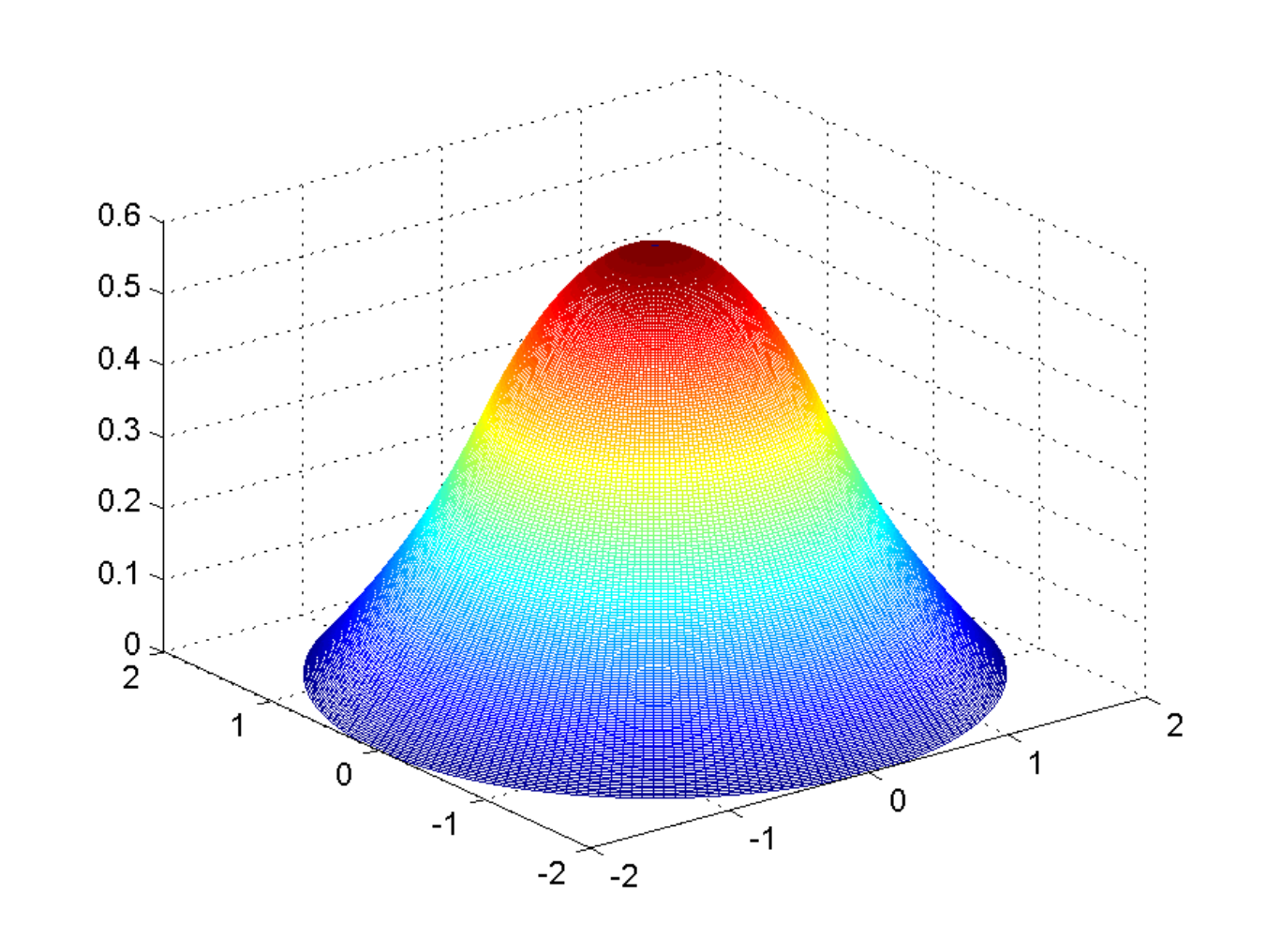
(a) exact state $y$

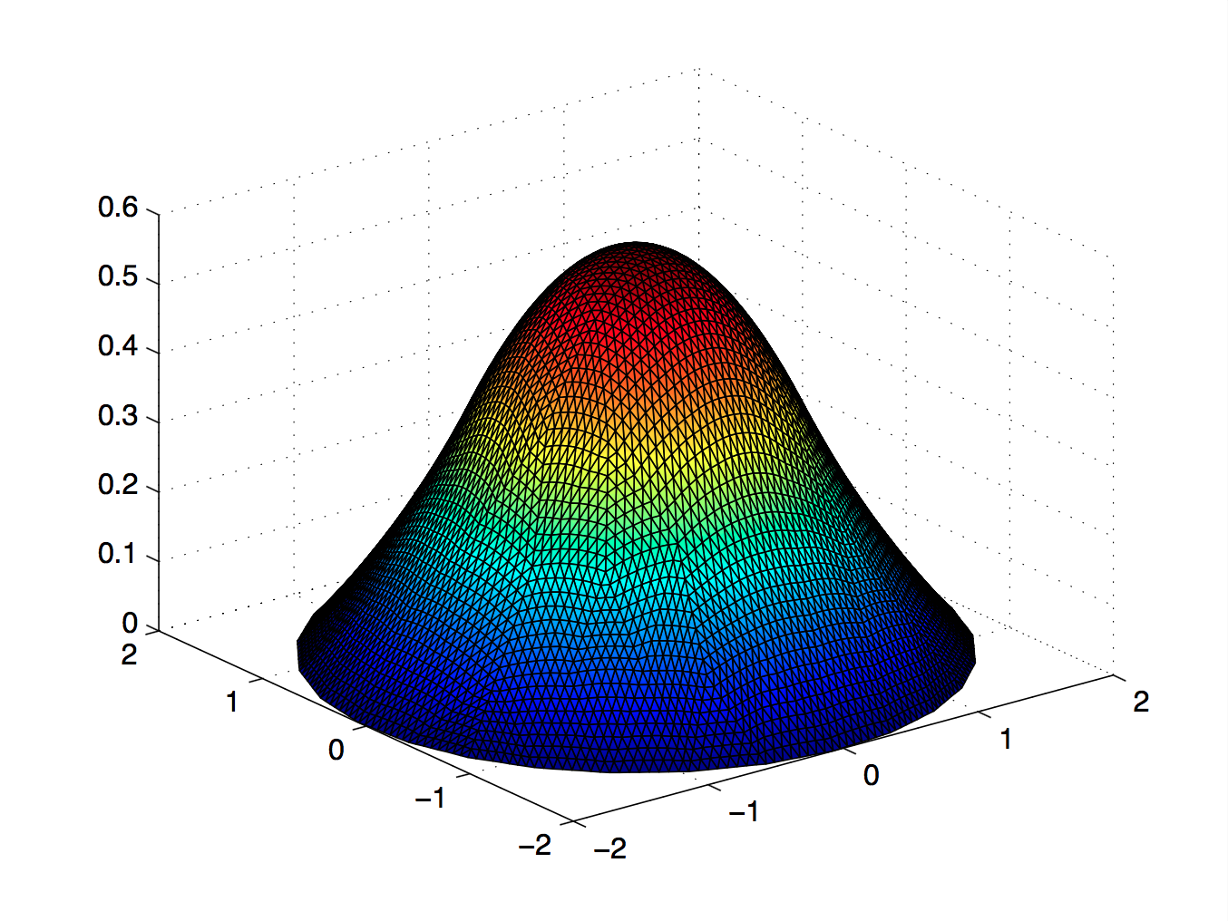
(b) numerical state $y_{h}$

Figure 1: Figures of exact and numerical state on the grid of size $h=\frac{1}{2^{5}}$ for Example 1.

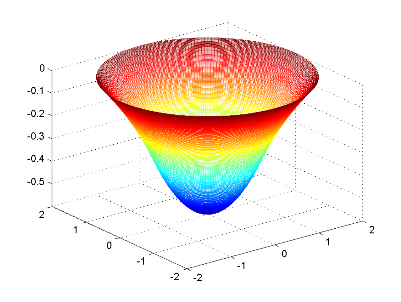
(a) exact control $u$

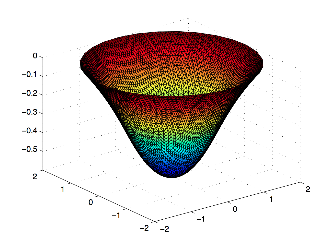
(b) numerical control $u_{h}$

Figure 2: Figures of exact and numerical control on the grid of size $h=\frac{1}{2^{5}}$ for Example 1.

Table 2: The performance of FE-dABCD algorithm for ($\mathrm{D\widetilde{P}}_{h}$) with different values of $\alpha$.

$h$			$\alpha$			iter			residual $\eta_{d}$
$\frac{1}{2^{6}}$			$10^{-2}$			16			9.28e-05
			$5\times 10^{-3}$			17			9.55e-05
			$10^{-3}$			19			8.48e-05
			$5\times 10^{-4}$			20			7.47e-05
			$10^{-4}$			21			9.27e-05
			$5\times 10^{-5}$			22			9.98e-05
			$10^{-5}$			25			3.81e-05

Example 2

In this example, we consider problem ($\mathrm{P}$) with the following data, $\mathrm{\Omega}=B_{1}(0)\subset\mathbb{R}^{2}$,

$$\mathcal{W}=\{u\in L^{\infty}(\mathrm{\Omega})|\ 0\leq u\leq\frac{1}{2}\quad\mathrm{a.e.}\ x\in\mathrm{\Omega}\},\quad\mathcal{K}=\{\mathbf{z}\in{L^{2}(\bar{\mathrm{\Omega}})}^{2}|\int_{\mathrm{\Omega}}\ |\mathbf{z}(x)|^{2}dx\leq\frac{1}{2}\}$$

as well as

$$y_{d}(x):=|x|^{2},\qquad 0\leq|x|\leq 1.$$

We consider the problem

$$-\mathrm{\Delta}y =u\quad\mathrm{in}\ \mathrm{\Omega},$$

$$y =0\quad\mathrm{on}\ \mathrm{\Gamma},$$

which means $f(x)=0$.

In this example, we still first focus on the convergence behavior of FE-dABCD algorithm compared with ihADMM algorithm and ADMM algorithm. In this case, we set $\alpha=10^{-2}$, $\epsilon=10^{-4}$ and $k_{m}=100$. The relative results are given in Table 3. Then, similar to Example 1, to show the robustness of our proposed FE-dABCD algorithm with respect to the parameter $\alpha$, we will also test the same problem with different values of $\alpha$, ranging from $10^{-2}$ to $10^{-5}$, on the grid of size $h=\frac{1}{2^{6}}$ and the corresponding results are presented in Table 4.

It is clear from Table 3 that the efficiency of our proposed FE-dABCD algorithm compared with ihADMM algorithm and ADMM algorithm. We can also see from the results in Table 3 that the number of iteration of FE-dABCD algorithm is independent of the discretization level. And from the results in Table 4, we can find that although the number of iterations of our proposed FE-dABCD algorithm increases obviously when $\alpha$ changes from $10^{-2}$ to $10^{-5}$, it still could solve problem ($\mathrm{D\widetilde{P}}_{h}$) for all tested values of $\alpha$ in $50$ iterations.

Table 3: The convergence behavior of FE-dABCD algorithm, ihADMM algorithm and ADMM algorithm for Example 2.

$h$			$\#$dofs						FE-dABCD			ihADMM			ADMM
						iter			10			30			30
$\frac{1}{2^{3}}$			273			residual $\eta$			7.83e-05			2.74e-05			7.74e-05
						time/s			0.0589			0.0669			0.0692
						iter			9			33			36
$\frac{1}{2^{4}}$			1145			residual $\eta$			3.56e-05			9.21e-05			2.06e-05
						time/s			0.2437			0.3238			0.4969
						iter			8			32			47
$\frac{1}{2^{5}}$			4689			residual $\eta$			7.57e-05			9.66e-05			8.96e-05
						time/s			0.9482			1.7690			3.6804
						iter			9			31			55
$\frac{1}{2^{6}}$			18977			residual $\eta$			3.39e-05			9.77e-05			2.17e-05
						time/s			6.2710			8.2806			24.7473
						iter			7			28			69
$\frac{1}{2^{7}}$			76353			residual $\eta$			8.36e-05			9.35e-05			6.49e-05
						time/s			32.7311			40.2470			217.994

Table 4: The performance of FE-dABCD algorithm for ($\mathrm{D\widetilde{P}}_{h}$) with different values of $\alpha$.

$h$			$\alpha$			iter			residual $\eta_{d}$
$\frac{1}{2^{6}}$			$10^{-2}$			9			3.39e-05
			$5\times 10^{-3}$			11			4.25e-05
			$10^{-3}$			15			7.38e-05
			$5\times 10^{-4}$			21			7.71e-05
			$10^{-4}$			30			7.38e-05
			$5\times 10^{-5}$			39			7.71e-05
			$10^{-5}$			46			7.38e-05

6 Conclusion

In this paper, we impose integral constraint on the gradient of the state and box constraints on the control. Our main results are proving the optimal conditions for the optimal control problem and also giving an efficient finite element duality-based inexact majorized accelerated block coordinate descent (FE-dABCD) algorithm. We consider piecewise linear approximation for both the state and the control and then transform the discretized problem into a multi-block unconstrained optimization problem by its dual. Our proposed method employs a majorization technique, which allow us to flexibly choose different proximal terms for different subproblems. Additionally, each subproblem only has to be solved approximately thanks to the inexactness of our proposed method. These flexibilities make each subproblem keep good structure and can be solved efficiently and reduce the cost for solving the subproblems largely, which improve the efficiency of our proposed method greatly. Specifically, we solve the smooth subproblem by GMRES method with preconditioner and solve nonsmooth subproblems through introducing appropriate proximal terms and semi-smooth Newton (SSN) method. We proved that the FE-dABCD algorithm enjoys $O(\frac{1}{k^{2}})$ iteration complexity. It is also easy to see the efficiency of FE-dABCD algorithm from the numerical results.

References

• (1) Axelsson, O. and Farouq, S. and Neytcheva, M.: Comparison of preconditioned Krylov subspace iteration methods for PDE-constrained optimization problems. Numer. Algorithms 73, 631–663 (2016)
• (2) Beck, A. and Teboulle, M.: A Fast Iterative Shrinkage-Thresholding Algorithm for Linear Inverse Problems. SIAM J. Imaging Sci. 2, 183–202 (2009)
• (3) Blumensath, T. and Davies, M.E.: Iterative Thresholding for Sparse Approximations. J. Fourier Anal. Appl. 14, 629–654 (2008)
• (4) Casas, E.: Boundary control of semilinear elliptic equations with pointwise state constraints. SIAM J. Control Optim. 31, 993–1006 (1993)
• (5) Casas, E. and Fern$\acute{a}$dez, L.A.: Optimal control of semilinear elliptic equations with pointwise constraints on the gradient of the state. Appl. Math. Optim. 27, 35–56 (1993)
• (6) Chambolle, A. and Pock, T.: A remark on accelerated block coordinate descent for computing the proximity operators of a sum of convex functions. J. Comput. Math. 1, 29–54 (2015)
• (7) Chen, L.: iFEM: an integrated finite element methods package in MATLAB. Technical report, University of California at Irvine. (2009)
• (8) Sun, D.F., Toh, K.C. and Yang, L.: An Efficient Inexact ABCD Method for Least Squares Semidefinite Programming. SIAM J. Optim. 26, 1072–1100 (2016)
• (9) Chen, Z.X., Song, X.L., Zhang, X.P. and Yu, B.: A FE-ADMM algorithm for Lavrentiev-regularized state-constrained elliptic control problem. ESAIM Control Optim. Calc. Var. (2018). https://doi.org/10.1051/cocv/2018019
• (10) Collis, S.S., Heinkenschloss, M., Scott, S. and Heinkenschloss, C.M.: Analysis of the Streamline Upwind/Petrov Galerkin Method Applied to the Solution of Optimal Control Problems. Technical Report TR02-01, Department of Computational and Applied Mathematics, Rice University, Houston, TX (2002)
• (11) Cui, Y.: Large scale composite optimization problems with coupled objective functions: theory, algorithms and applications. Ph.D. thesis (2016)
• (12) Deckelnick, K. and Hinze, M.: A-Priori Error Bounds for Finite Element Approximation of Elliptic Optimal Control Problems with Gradient Constraints. Internat. Ser. Numer. Math. 165, 365–382 (2014)
• (13) Grippo, L. and Sciandrone, M.: On the convergence of the block nonlinear Gauss-Seidel method under convex constraints. Oper. Res. Lett. 26, 127–136 (2000)
• (14) Hintermüller, M. and Kunisch, K.: Boundary control of semilinear elliptic equations with discontinuous leading coefficients and unbounded controls. SIAM J. Control Optim. 45, 1198–1221 (2006)
• (15) Hintermüller, M. and Kunisch, K.: Path-following methods for a class of constrained minimization problems in function space. SIAM J. Optim. 17, 159–187 (2006)
• (16) Hinze, M. and Christian, M.: Variational discretization of Lavrentiev-regularized state constrained elliptic optimal control problems. Comput. Optim. Appl. 46, 487–510 (2010)
• (17) Hinze, M., Pinnau, R., Ulbrich, M. and Ulbrich, S.: Optimization with PDE constraints. Springer Netherlands (2009).
• (18) Hiriart-Urruty, J.B. and Strodiot, J.J. and Nguyen, V.H.: Generalized Hessian matrix and second-order optimality conditions for problems with $C^{1,1}$ data. Appl. Math. Optim. 11, 43–56 (1984)
• (19) Itoa, K. and Kunisch, K.: Semi-smooth Newton methods for state-constrained optimal control problems. Systems Control Lett. 50, 221–228 (2003)
• (20) Jiang, K.F., Sun D.F. and Toh, K.C.: An Inexact Accelerated Proximal Gradient Method for Large Scale Linearly Constrained Convex SDP. SIAM J. Optim. 22, 1042–1064 (2012)
• (21) Kunisch, K., Liang, K. and Lu, X.: Optimal Control for an Elliptic System with Polygonal State Constraints. SIAM J. Control Optim. 48, 5053–5072 (2010)
• (22) Li, X.D., Sun, D.F. and Toh, K.C.: QSDPNAL: A two-phase Newton-CG proximal augmented Lagrangian method for convex quadratic semidefinite programming problems. arXiv preprint arXiv:1512.08872 (2015)
• (23) Li, X.D., Sun, D.F. and Toh, K.C.: A Schur complement based semi-proximal ADMM for convex quadratic conic programming and extensions. Math. Program. 155, 333–373 (2016)
• (24) Meyer, C., Sch, A. and Ltzsch, F.: Optimal Control of PDEs with Regularized Pointwise State Constraints. Comput. Optim. Appl. 33, 209–228 (2006)
• (25) Nther, A. and Hinze, M.: Elliptic control problems with gradient constraints-variational discrete versus piecewise constant controls. Comput. Optim. Appl. 49, 549–566 (2011)
• (26) Pr$\ddot{u}$fert, U.: On two numerical methods for state-constrained elliptic control problems. Optim. Methods Softw. 22, 871–899 (2007)
• (27) Sardy, S., Bruce, A.G. and Tseng, P.: Block coordinate relaxation methods for nonparametric wavelet denoising. J. Comput. Graph. Statist. 9, 361–379 (2000)
• (28) Schindele, A. and Borzì, A.: Proximal Methods for Elliptic Optimal Control Problems with Sparsity Cost Functional. Applied Mathematics 7, 967–992 (2016)
• (29) Song, X.L. and Chen, B. and Yu, B.: An efficient duality-based approach for PDE-constrained sparse optimization. Comput. Optim. Appl. 69, 461–500 (2018)
• (30) Song, X.L. and Yu, B.: A two-phase method for control constrained elliptic optimal control problem. Numer. Linear Algebra Appl. 25, e2138 (2018)
• (31) Song, X.L., Yu, B., Wang, Y.Y. and Zhang, X.P.: A FE-inexact heterogeneous ADMM for Elliptic Optimal Control Problems with $L^{1}$-Control Cost. J. Syst. Sci. Complex. (2017). DOI: 10.1007/s11424-018-7448-6
• (32) Sun, D.F., Toh, K.C. and Yang, L.Q.: An Efficient Inexact ABCD Method for Least Squares Semidefinite Programming. SIAM J. Optim. 26, 1072–1100 (2016)
• (33) Toh, K.C. and Yun, S.: An accelerated proximal gradient algorithm for nuclear norm regularized linear least squares problems. Pac. J. Optim. 6, 615–640 (2010)
• (34) Tseng, P.: Convergence of a Block Coordinate Descent Method for Nondifferentiable Minimization. J. Optim. Theory Appl. 109, 475–494 (2001)
• (35) Tseng, P.: Dual coordinate ascent methods for non-strictly convex minimization. Math. Program. 59, 231–247 (1993)
• (36) Wathen, A.J.: Realistic Eigenvalue Bounds for the Galerkin Mass Matrix. IMA J. Numer. Anal. 7, 449–457 (1987)
• (37) Wollner, W.: A Priori Error Estimates for Optimal Control Problems with Constraints on the Gradient of the State on Nonsmooth Polygonal Domains. Internat. Ser. Numer. Math. 164, 193–215 (2013)