$\mathbb{Z}_{2}$-equivariant Heegaard Floer cohomology of knots in $S^{3}$ as a strong Heegaard invariant

Abstract.

The $\mathbb{Z}_{2}$-equivariant Heegaard Floer cohomlogy $\widehat{HF}_{\mathbb{Z}_{2}}(\Sigma(K))$ of a knot $K$ in $S^{3}$, constructed by Hendricks, Lipshitz, and Sarkar, is an isotopy invariant which is defined using bridge diagrams of $K$ drawn on a sphere. We prove that $\widehat{HF}_{\mathbb{Z}_{2}}(\Sigma(K))$ can be computed from knot Heegaard diagrams of $K$ and show that it is a strong Heegaard invariant. As a topolocial application, we construct a transverse knot invariant $\hat{\mathcal{T}}_{\mathbb{Z}_{2}}(K)$ as an element of $\widehat{HFK}_{\mathbb{Z}_{2}}(\Sigma(K),K)$, which is a refinement of $\widehat{HF}_{\mathbb{Z}_{2}}(\Sigma(K))$, and show that it is a refinement of both the LOSS invariant $\hat{\mathcal{T}}(K)$ and the $\mathbb{Z}_{2}$-equivariant contact class $c_{\mathbb{Z}_{2}}(\xi_{K})$.

1. Introduction

Suppose that a based knot $K$ in $S^{3}$ is given. Then we can represent $K$ as a bridge diagram on a sphere, and taking its branched double cover along the points where $K$ and the sphere intersect gives a Heegaard diagram of the branched double cover $\Sigma(K)$ of $S^{3}$ along $K$. This diagram admits a natural $\mathbb{Z}_{2}$-action which fixes the basepoint and the $\alpha$,$\beta$-curves. From these data, Hendricks, Lipshitz, and Sarkar[HLS] gave a construction of the $\mathbb{Z}_{2}$-equivariant Heegaard Floer cohomology $\widehat{HF}_{\mathbb{Z}_{2}}(\Sigma(K))$, using their formulation of $\mathbb{Z}_{2}$-equivariant Floer cohomology theory. They also proved that the isomorphism class of $\widehat{HF}_{\mathbb{Z}_{2}}(\Sigma(K))$, which is a $\mathbb{F}_{2}[\theta]$-module where $\theta$ is a formal variable, is an invariant of the isotopy class of the given knot $K$. Also, the author proved in [K] that $\widehat{HF}_{\mathbb{Z}_{2}}(\Sigma(K))$ satisfies naturality and is functorial under based link cobordisms whose ends are knots.

Given these facts, it is natural to ask whether $\widehat{HF}_{\mathbb{Z}_{2}}(\Sigma(K))$ can be computed from bridge diagrams of $K$ drawn on closed surfaces of aribtrary genera, instead of spheres. In section 2, we will see that this is almost always possible, by proving the following theorem.

Theorem 1.1.

Let $\mathcal{E}$ be a weakly admissible extended bridge diagrams representing a knot in $S^{3}$, which has at least two A-arcs. Then $\widehat{HF}_{\mathbb{Z}_{2}}(\mathcal{E})\simeq\widehat{HF}_{\mathbb{Z}_{2}}(\Sigma(K))$.

Now, given such a fact, we can use it to compute $\widehat{HF}_{\mathbb{Z}_{2}}(\Sigma(K))$ from a weakly admissible knot Heegaard diagram of $K$. To write it up clearly, choose a weakly admissible knot Heegaard diagram $H=(\Sigma,\boldsymbol{\alpha},\boldsymbol{\beta},z,w)$ which represents a based knot $(K,z)$. Add a pair of a small A-arc and a small B-arc connected to $w$, whose interiors are disjoint; this gives a weakly admissible extended bridge diagram representing $K$, which has at least two A-arcs. Then taking the branched double cover of the resulting extended bridge diagram and forgetting all basepoints except $z$ gives a Heegaard diagram of $\Sigma(K)$ together with a $\mathbb{Z}_{2}$-action. By Theorem 1.1, the $\mathbb{Z}_{2}$-equivariant Heegaard Floer cohomology of this diagram is isomorphic to $\widehat{HF}_{\mathbb{Z}_{2}}(\Sigma(K))$.

This construction implies that $\widehat{HF}_{\mathbb{Z}_{2}}(\Sigma(K))$ is a weak Heegaard invariant of $K$, as defined in [JT]. In section 3, we will see that the $\mathbb{Z}_{2}$-equivariant Heegaard Floer cohomology, as a weak Heegaard invariant, satisfies certain commutativity axioms, thereby proving that it is actually a strong Heegaard invariant. Morover, we will also see that $\widehat{HF}_{\mathbb{Z}_{2}}$ as a natural invariant calculated from bridge diagrams on a sphere is naturally isomorphic to $\widehat{HF}_{\mathbb{Z}_{2}}$ as a strong Heegaard invariant; to be precise, we will prove the following theorem.

Theorem 1.2.

Consider the category $\text{Knot}_{\ast}$ whose objects are based knots in $S^{3}$ and morphisms are self-diffeomorphisms of $S^{3}$, and let

$$\widehat{HF}_{\mathbb{Z}_{2}}^{bridge}\,:\,\text{Knot}_{\ast}\rightarrow\text{Mod}_{\mathbb{F}_{2}[\theta]}$$

be the functor defined in Theorem 6.9 of [K]. Also, let

$$\widehat{HF}_{\mathbb{Z}_{2}}^{knot}\,:\,\text{Knot}_{\ast}\rightarrow\text{Mod}_{\mathbb{F}_{2}[\theta]}$$

be the functor defined by considering $\widehat{HF}_{\mathbb{Z}_{2}}$ as a strong Heegaard invariant. Then there exists an invertible natural transformation between $\widehat{HF}_{\mathbb{Z}_{2}}^{bridge}$ and $\widehat{HF}_{\mathbb{Z}_{2}}$.

In section 4, we will see that any knot Heegaard diagrams representing a (based) knot $K$ in $S^{3}$ can be transformed, via isotopies and handleslides, to certain types of knot Heegaard diagrams, called very nice diagrams. Also, we will see that, from such a diagram, we can compute $\widehat{HF}_{\mathbb{Z}_{2}}(\Sigma(K))$ in a purely combinatorial way. As a result, we can remove a pair of an A-arc and a B-arc when computing $\widehat{HF}_{\mathbb{Z}_{2}}$ from a knot Heegaard diagram, and thus extend Theorem 1.1 to full generality.

Theorem 1.3.

Let $\mathcal{E}$ be a weakly admissible extended bridge diagrams representing a knot in $S^{3}$. Then $\widehat{HF}_{\mathbb{Z}_{2}}(\mathcal{E})\simeq\widehat{HF}_{\mathbb{Z}_{2}}(\Sigma(K))$.

In section 5, we construct a new invariant $\widehat{HFK}_{\mathbb{Z}_{2}}(\Sigma(K),K)$ associated to a knot $K$ in $S^{3}$, whose isomorphism class is also an invariant of the isotopy class of $K$, and prove that a version of localization isomorphism exists for $\widehat{HFK}_{\mathbb{Z}_{2}}$. Finally, in section 6, we will construct an element $\hat{\mathcal{T}}_{\mathbb{Z}_{2}}(K)\in\widehat{HFK}_{\mathbb{Z}_{2}}(\Sigma(K),K)$ associated to a transverse knot $K$ in the standard contact sphere $(S^{3},\xi_{std})$, which depends only on the transverse isotopy class of $K$, and see that it is a refinement of both the LOSS invariant defined in [LOSSz] and the $\mathbb{Z}_{2}$-equivariant contact class defined by the author in [K].

Acknowledgement

The author would like to thank Andras Juhasz and Robert Lipshitz for helpful discussions and suggestions.

2. Equivariant Heegaard Floer cohomology and extended bridge diagrams

Definition 2.1.

Suppose that a Heegaard diagram $\mathcal{H}=(\Sigma,\boldsymbol{\alpha},\boldsymbol{\beta})$ is given. A based bridge diagram on $\mathcal{H}$ is a 4-tuple $(F,A,B,z)$, where $F\subset\Sigma$ is a finite subset of points in $\Sigma$, $A,B$ are sets of simple arcs on $\Sigma$, and $z\in F$, such that the following properties are satisfied.

• For any $\gamma\in\boldsymbol{\alpha}\cup\boldsymbol{\beta}$, we have $F\cap\gamma=\emptyset$.

• For any two distinct elements $\boldsymbol{a},\boldsymbol{a}^{\prime}\in A\cup\boldsymbol{\alpha}$, we have $\boldsymbol{a}\cap\boldsymbol{a}^{\prime}=\emptyset$, and the same statement holds for elements in $B\cup\boldsymbol{\beta}$.

• For any $\boldsymbol{a}\in A\cup\boldsymbol{\alpha}$ and $\boldsymbol{b}\in B\cup\boldsymbol{\beta}$, the intersection $\boldsymbol{a}\cap\boldsymbol{b}$ is transverse.

• For any $\boldsymbol{c}\in A\cup B$, the two endpoints of $\boldsymbol{c}$ are distinct and $\boldsymbol{c}\cap F=\partial\boldsymbol{c}$.

• For any $p\in F$, there exists a unique element $\boldsymbol{a}$ of $A$ which satisfies $p\in\partial\boldsymbol{a}$, and the same statement holds for $B$.

Given a pointed bridge diagram $(F,A,B,z)$ on a Heegaard diagram $(\Sigma,\boldsymbol{\alpha},\boldsymbol{\beta})$, we call the elements of $A$ as A-arcs, the elements of $B$ as B-arcs, and $z$ as the basepoint. Note that $(\Sigma,\boldsymbol{\alpha},\boldsymbol{\beta},z)$ is a pointed Heegaard diagram.

Suppose that a Heegaard diagram $\mathcal{H}=(\Sigma,\boldsymbol{\alpha},\boldsymbol{\beta})$ describes a 3-manifold $M$. Then, given a based bridge diagram $\mathcal{P}=(F,A,B,z)$ on $\mathcal{H}$, we can construct a based link $(L,p)$ lying inside $M$ as follows. Let $M=H_{1}\cup H_{2}$ be a Heegaard splitting of $M$ given by the Heegaard surface $\Sigma$. Suppose that we call $H_{1}$ as the “outside” of $\Sigma$ and $H_{2}$ as the “inside” of $\Sigma$. Then, we can isotope the A-arcs of $\mathcal{P}$ slightly ourwards and the B-arcs of $\mathcal{P}$ slightly inwards, while leaving the set $F$ fixed. Concatenating the isotoped arcs gives us a link $L\subset M$, and the basepoint $p$ lies on $L$, so that we get a based link $(L,p)$ in $M$, which is uniquely determined up to (based) isotopy.

Definition 2.2.

Suppose that a Heegaard diagram $\mathcal{H}=(\Sigma,\boldsymbol{\alpha},\boldsymbol{\beta})$ describes a 3-manifold $M$. We say that a based link $(L,p)$ in $M$ is represented by a based bridge diagram $\mathcal{P}=(F,A,B,z)$ if the process described above gives a based link which is (based) isotopic to $(L,p)$.

Proposition 2.3.

Suppose that a Heegaard diagram $\mathcal{H}=(\Sigma,\boldsymbol{\alpha},\boldsymbol{\beta})$ describes a 3-manifold $M$. Then every based link in $M$ can be represented by a based bridge diagram on $\mathcal{H}$.

Proof.

Let $M=H_{1}\cup H_{2}$ be the Heegaard splitting of $M$, induced by $\mathcal{H}$. Then for each $i=1,2$, there exists a 1-subcomplex $C_{i}\subset\text{int}(H_{i})$ so that $H_{1}-C_{1}\simeq\Sigma\times[0,\infty)$ and $H_{2}-C_{2}\simeq\Sigma\times(-\infty,0]$. Since $C_{1}$ and $C_{2}$ are both 1-dimensional and $M$ is a 3-manifold, we can isotope $(L,p)$ so that $p\in\Sigma$, $L$ does not intersect $C_{1}\cup C_{2}$ and $L$ intersect transversely with $\Sigma$. After further isotoping $L$, we may assume that every component $c^{i}$ of $L\cap H_{i}$ admits a disk $D_{c^{i}}\subset H_{i}$ so that $c^{i}\subset\partial D_{c^{i}}\subset c^{i}\cup\Sigma$, and for any two distinct components $c_{1}^{i},c_{2}^{i}$ of $L\cap H_{i}$, we have $D_{c_{1}^{i}}\cap D_{c_{2}^{i}}=\emptyset$. We can also assume that the disks $D_{c^{i}}$ does not intersect the family of compressing disks in $H_{i}$ , determined by the alpha- and beta-curves of $\mathcal{H}$, possibly after applying another isotopy to $L$, while leaving the basepoint $p$ fixed. For each component $c^{i}\in\pi_{0}(L\cap H_{i})$, write $\partial D_{c^{i}}=c^{i}\cup p(c^{i})$ where $u^{i}\subset\Sigma$, i.e. $p(c^{i})$ is a simple arc on $\Sigma$ which is a projection of $c^{i}$. By assumption, the arcs $p(c^{i})$ does not intersect the alpha- or beta-curves, and any two distinct arcs $p(c_{1}^{i})$ and $p(c_{2}^{i})$ do not intersect.

Now, after isotoping the arcs $p(c^{i})$, we can assume that for any two curves $p(c^{i})$ and $p(c^{j})$ intersect transversely if $i\neq j$, i.e. $\{i,j\}=\{1,2\}$. Consider the following sets:

$$A =\{p(c)\,|\,c\in\pi_{0}(L\cap H_{1})\},$$

$$B =\{p(c)\,|\,c\in\pi_{0}(L\cap H_{2})\},$$

$$F =\bigcup_{u\in A\cup B}\partial u.$$

Then $p\in F$, and the based bridge diagram $(A,B,F,p)$ represents the given based link $(L,p)$ in $M$. ∎

Definition 2.4.

An extended bridge diagram is a pair $\mathcal{E}=(\mathcal{H},\mathcal{P})$, where $\mathcal{H}$ is a Heegaard diagram and $\mathcal{P}$ is a based bridge diagram on $\mathcal{H}$. We write $\mathcal{H}$ as $\mathcal{H}(\mathcal{E})$ and $\mathcal{P}$ as $\mathcal{P}(\mathcal{E})$. If $\mathcal{H}=(\Sigma,\boldsymbol{\alpha},\boldsymbol{\beta})$ and $\mathcal{P}=(A,B,F,p)$, the pointed Heegaard diagram $(\Sigma,\boldsymbol{\alpha},\boldsymbol{\beta},p)$ will be denoted as $\mathcal{H}_{st}(\mathcal{E})$. Also, the 3-manifold represented by $\mathcal{H}$ is denoted as $M(\mathcal{E})$, and the based link in $M(\mathcal{E})$ represented by $\mathcal{P}$ is denoted as $L(\mathcal{E})$.

Given an extended bridge diagram $\mathcal{E}=(\mathcal{H},\mathcal{P})$, we have an associated 3-tuple $(M,L,p)$, where $M$ is the 3-manifold represented by $\mathcal{H}$, and $(L,p)$ is a based link in $M$, represented by $\mathcal{P}$. Obviously, given a 3-maniold together with a based link inside it, we have lots of extended bridge diagrams which represents it. In particular, we have a set of operations on extended bridge diagrams which leave the associated 3-manifold and based link fixed, which we will call as extended Heegaard moves. Also, we will call isotopies and handleslides involving $\alpha$($\beta$)-curves as $\alpha$($\beta$)-equivalences, and those involving A(B)-arcs and A(B)-equivalences. Finally, we will call $\alpha$,$\beta$-equivalences and A,B-equivalences as basic moves.

Isotopies

Given an extended bridge diagram, we can isotope its A-arcs, B-arcs, alpha-curves and beta-curves.

Handleslides of type I

Given an extended bridge diagram, we can replace an alpha(beta)-curve $\alpha$ with another simple closed curve $\alpha^{\prime}$ through an ordinary handleslide of knot Heegaard diagrams. Here, the handleslide region must not intersect any of the A/B-arcs.

Handleslides of type II

Given an extended bridge diagram, we can replace an alpha(beta)-curve $\alpha$ with another simple closed curve $\alpha^{\prime}$ if the following conditions are satisfied.

• The curve $\alpha^{\prime}$ does not intersect with any of the A(B)-arcs and the alpha(beta)-curves.

• There exists an A-arc $A$ so that $\alpha,\alpha^{\prime}$ cobound a cylinder whose interior contains $A$ and does not intersect with any of the A-arcs, B-arcs, alpha-curves, and the beta-curves, except $A$.

Handleslides of type III

Given an extended bridge diagram, we can replace an A(B)-arc $a$ with another simple arc $a^{\prime}$ if the following conditions are satisfied.

• $\partial a=\partial a^{\prime}$.

• The interior of $a^{\prime}$ does not intersect with any of the A(B)-arcs and the alpha(beta)-curves.

• There exists an alpha(beta)-curve $\alpha$ so that $a,a^{\prime},\alpha$ bound a cylinder $C\subset\Sigma$, whose interior does not intersect with any of the A-arcs, B-arcs, alpha-curves, and the beta-curves.

Handleslides of type IV

Given an extended bridge diagram, we can replace an A(B)-arc $a$ with another simple arc $a^{\prime}$ if the following conditions are satisfied.

• The interior of $a^{\prime}$ does not intersect with any of the A(B)-arcs and the alpha(beta)-curves.

• There exists an A(B)-arc $a_{0}$ such that $a,a^{\prime}$ bound a disk $D\subset\Sigma$, whose interior contains $a_{0}$ and does not intersect with any of the A-arcs, B-arcs, alpha-curves, and the beta-curves, except for $a_{0}$.

(De)stabilizations of type I

Given an extended bridge diagram $((\Sigma,\boldsymbol{\alpha},\boldsymbol{\beta}),(F,A,B,p))$, we can stabilize its Heegaard diagram $(\Sigma,\boldsymbol{\alpha},\boldsymbol{\beta})$ at a point $q\in\Sigma$ such that $q\notin c$ for any $c\in A\cup B$. The based bridge diagram $(F,A,B,p)$ remains the same.

(De)stabilizations of type II

Given an extended bridge diagram $((\Sigma,\boldsymbol{\alpha},\boldsymbol{\beta}),(F,A,B,p))$, where $|F|>2$, choose an A-arc $a$ such that $p\notin\partial a$, and pick one of its endpoints, $z\in\partial a$. Choose two distinct points $x,y$ lying in the interior of $z$, so that the following conditions hold.

• $a-\{x,y\}$ has three components $a_{1},b_{1},a^{\prime}$, which are simple arcs on $\Sigma$.

• $\partial a_{1}=\{z,x\}$, $\partial b_{1}=\{x,y\}$, and $\partial a^{\prime}=\{y\}\cup(\partial a-\{z\})$.

• $a_{1}$ and $b_{1}$ do not intersect with any of the B-arcs and beta-curves.

Then $((\Sigma,\boldsymbol{\alpha},\boldsymbol{\beta}),(F\cup\{x,y\},(A-\{a\})\cup\{a_{1},a^{\prime}\}),B\cup\{b_{1}\},p))$ is again an extended bridge diagram.

Diffeomorphism

Given an extended bridge diagram $((\Sigma,\boldsymbol{\alpha},\boldsymbol{\beta}),(F,A,B,p))$ and a diffeomorphism $\phi\in\text{Diff}^{+}(\Sigma)$, we can apply $\phi$ on everything to get another extended bridge diagram.

Proposition 2.5.

Let $\mathcal{H}=(\Sigma,\boldsymbol{\alpha},\boldsymbol{\beta})$ be a Heegaard diagram which represent a 3-manifold $M$. Any two based bridge diagrams on $\mathcal{H}$, which represent isotopic based links in $M$, are related by isotopies, handleslides of type II, III, IV, and (de)stabilizations of type II.

Proof.

Choose a pair of a self-indexing Morse function $f:M\rightarrow[0,3]$ and a Riemannian metric $g$ on $M$, which induces the Heegaard diagram $\mathcal{H}$ of $M$. In the space $\mathcal{S}$ of based link $M$ such that its basepoint lies on $\Sigma$ and it is transverse to $\Sigma$ at the basepoint, the subspace $\mathcal{S}_{0}$ of based links $(L,p)$ which satisfy the conditions below is open and dense. Given any link in $\mathcal{S}_{0}$, its projection along the gradient flow of $f$ gives a based bridge diagram of $(L,p)$ on $\mathcal{H}$, up to stabilizations of type II.

• The intersection $L\cap\Sigma$ is transverse.

• The gradient vector field $\nabla_{g}f$ is nonvanishing on $L$ and transverse to $L$.

• For any flowline $c$ of $\nabla_{g}f$ whose endpoints lie on $L$, the intersection $c\cap\Sigma$ is transverse.

• For each bi-infinite flowline $\gamma$ of $\nabla_{g}f$, we have $|\gamma\cap L|\leq 2$, and if the equality holds, we have $\gamma\cap\Sigma\cap L=\emptyset$.

• The intersections of $L$ with the unstable manifolds of critical points of index $2$ and the stable manifolds of critical points of index $1$ are transverse.

We call the set $\mathcal{S}_{0}$ as the set of points of codimension $0$; to prove the proposition, it suffices to classify the codimension $1$ singularities inside $\mathcal{S}$ and show that they correspond to (compositions of) handleslides of type II, III, IV, and stabilizations of type II. It is easy to see that the codimension $1$ singularities in $\mathcal{S}$ are given as follows.

1. The link $L$ is tangent to $\Sigma$ at a point $z\in\Sigma$, such that $z\neq p$ and the order of tangency is $1$.

2. The link $L$ intersects transversely with either the stable manifold of a critical point of index $2$ or the unstable manifold of a critical point of index $1$.

3. There exists a flowline $\gamma$ of $\nabla_{g}f$ which is tangent to $L$ at a point, such that the order of tangency is $1$.

4. There exists a bi-infinite flowline $\gamma$ of $\nabla_{g}f$ such that $|\gamma\cap L|=2$ and $|\gamma\cap\Sigma\cap L|=1$.

5. The link $L$ is tangent to either the unstable manifold of a critical point of index $2$ or the stable manifold of a critical point of index $1$, such that the order of tangency is $1$.

6. There exists three distinct points $x,y,z\in\Sigma$, different from the basepoint $p$, and a bi-infinite flowline $\gamma$ of $\nabla_{g}f$ such that $x,y,z\in\gamma$.

The perturbations of the above singularities can be translated as the following compositions of extended Heegaard moves.

1. A single stabilization of type II.

2. A single handleslide of type III.

3. The composition of two stabilization of type II and a handleslide of type II.

4. The composition of a stabilization of type II and a handleslide of type IV.

5. An isotopy.

6. The composition of a stablilization of type II, a handleslide of type IV, and an isotopy.

Therefore we see that any two based bridge diagrams on $\mathcal{H}$ which represent isotopic based links in $M$ are related by isotopies, handleslides of type II, III, IV, and (de)stabilizations of type II. ∎

Definition 2.6.

A based bridge diagram $\mathcal{P}$ on a Heegaard diagram $\mathcal{H}=(\Sigma,\boldsymbol{\alpha},\boldsymbol{\beta})$ is simple if all A-arcs and B-arcs of $\mathcal{P}$ lie in the same connected component of $\Sigma-\left(\bigcup_{\gamma\in\boldsymbol{\alpha}\cup\boldsymbol{\beta}}\gamma\right)$.

Theorem 2.7.

If two extended bridge diagrams which represent the same 3-manifold and isotopic based links, which are contained in a ball, they are related by extended Heegaard moves.

Proof.

Since the given link is assumed to be contained in a ball, for any Heegaard diagram $\mathcal{H}$, there exists a simple based bridge diagram $\mathcal{P}_{0}$ which also represents the given link. Now, given any based bridge diagram $\mathcal{P}$ on a Heegaard diagram $\mathcal{H}$, we know from Proposition 2.5 that we can apply isotopies, handleslides of type II, III, IV, and (de)stabilizations of type II to $\mathcal{P}$ to reach $\mathcal{P}_{0}$. But then, we can regard the A-arcs and B-arcs together as a “big basepoint” and apply isotopies, handleslides, stabilizations and diffeomorphisms to the Heegaard diagram $\mathcal{H}$. The handleslides and stabilizations applied to $\mathcal{H}$ corresponds to handleslides of type I and stabilizations of type I applied to the extended bridge diagram $(\mathcal{P},\mathcal{H})$. Since any two Heegaard diagrams representing the same 3-manifold are related by isotopies, handleslides, stabilizations, and diffeomorphisms, the proof is complete. ∎

Remark.

By considering perturbations of Morse-Smale pairs on $M$ together with perturbations of the given link $L$, and classifying all possible codimension $1$ singularities, we can remove the the assumption that our base link is contained in a ball, in Theorem 2.7. However, this observation is not necessary, as we will only consider knots and links in $S^{3}$ throughout this paper.

Now suppose that an extended bridge diagram $\mathcal{E}=(\mathcal{H},\mathcal{P})$, $\mathcal{H}=(\Sigma,\boldsymbol{\alpha},\boldsymbol{\beta})$, $\mathcal{P}=(F,A,B,z)$ is given, where the Heegaard diagram $\mathcal{H}$ represents a 3-manifold $M$ and the based bridge diagram $\mathcal{P}$ represents the isotopy class of a based link $(L,z)$ in $M$. Then we construct a $4$-tuple $\mathcal{H}_{d}(\mathcal{E})=(\tilde{\Sigma},\tilde{\boldsymbol{\alpha}},\tilde{\boldsymbol{\beta}},z)$, which is defined as follows.

• $\tilde{\Sigma}$ is the branched double cover of $\Sigma$ along $F$.

• $\tilde{\boldsymbol{\alpha}}=\left(\bigcup_{\alpha\in\boldsymbol{\alpha}}\{\text{connected components of }\alpha\}\right)\cup\{p^{-1}(a)\,|\,a\in A,\,z\notin\partial a\}$, where $p\,:\,\tilde{\Sigma}\rightarrow\Sigma$ is the branched covering map, and $\tilde{\boldsymbol{\beta}}$ is defined similarly.

• $z$ is the basepoint of the based link $(L,z)$.

The $4$-tuple $\mathcal{H}_{d}(\mathcal{E})$, by construction, is a Heegaard diagram for the based 3-manifold $(\Sigma_{L}(M),z)$, which is the branched double cover of the based 3-manifold $(M,z)$ along the link $L$. The covering transformation of the branched cover $\Sigma_{L}(M)\rightarrow M$ induces an orientation-preserving $\mathbb{Z}_{2}$-action on $\mathcal{H}_{d}(\mathcal{E})$. We will say that $\mathcal{H}_{d}(\mathcal{E})$ is the branched double cover of $\mathcal{H}$ along $\mathcal{P}$.

Proposition 2.8.

For any extended bridge diagram $\mathcal{E}$, the pointed Heegaard diagarm $\mathcal{H}_{d}(\mathcal{E})$ is weakly admissible if $\mathcal{H}_{pt}(\mathcal{E})$ is weakly admissible.

Proof.

We will continue using the notations which we have used above. Consider the branched covering map $p_{\Sigma}:\tilde{\Sigma}\rightarrow\Sigma$. Then, for any connected component $R$ of $\Sigma-\left(\bigcup_{c\in\boldsymbol{\alpha}\cup\boldsymbol{\beta}}c\right)$, which does not contain the basepoint $z$, we define its pullback $p_{\Sigma}^{\ast}(R)$ as follows.

• If $p_{\Sigma}^{-1}(R)$ is connected, it is a connected component of $\tilde{\Sigma}-\left(\bigcup_{\tilde{c}\in\tilde{\boldsymbol{\alpha}}\cup\tilde{\boldsymbol{\beta}}}\tilde{c}\right)$, so we define $p_{\Sigma}^{\ast}(R)$ as $p_{\Sigma}^{-1}(R)$.

• If $p_{\Sigma}^{-1}(R)$ is disconnected, it consists of a $\mathbb{Z}_{2}$-orbit of some connected component of $\tilde{\Sigma}-\left(\bigcup_{\tilde{c}\in\tilde{\boldsymbol{\alpha}}\cup\tilde{\boldsymbol{\beta}}}\tilde{c}\right)$, where $\mathbb{Z}_{2}$ acts as covering transformations. Denote that orbit as $\{T,\sigma T\}$, where $\mathbb{Z}_{2}=\left\langle\sigma\right\rangle$. Then we define $p_{\Sigma}^{\ast}(R)$ as $T+\sigma T$.

This definition can be extended linearly to give a group homomorphism

$$p_{\Sigma}^{\ast}:\mathcal{D}(\mathcal{H}_{pt}(\mathcal{E}))\rightarrow\mathcal{D}(\mathcal{H}_{d}(\mathcal{E})),$$

where $\mathcal{D}(\mathcal{H})$ for a point Heegaard diagram $\mathcal{H}$ is defined to be the free abelian group of domains in $\mathcal{H}$ which do not intersect the basepoint. The map $p_{\Sigma}^{\ast}$ clearly preserves periodicity.

Suppose that $\mathcal{H}_{pt}(\mathcal{E})$ is weakly admissible and there exists a positive periodic domain $D\in\mathcal{D}(\mathcal{H}_{d}(\mathcal{E}))$. Then $D+\sigma D$ is also a positive periodic domain in $\mathcal{H}_{d}(\mathcal{E})$. Using the proof of Lemma 4.2 in [K], we see that there exists a positive periodic domain $D_{0}\in\mathcal{D}(\mathcal{H}_{pt}(\mathcal{E}))$ such that $p_{\Sigma}^{\ast}D_{0}=D+\sigma D$. Since $\mathcal{H}_{pt}(\mathcal{E})$ is assumed to be weakly admissible, we must have $D_{0}=0$ and thus $D+\sigma D=0$. Since both $D$ and $\sigma D$ are positive, this implies $D=0$, a contradiction. Therefore $\mathcal{H}_{d}(\mathcal{E})$ must be weakly admissible. ∎

We will now proceed to weak admissibilities of Heegaard triple diagrams and quadruple diagrams, which are perturbations of branched double covers of extended bridge diagrams. More precisely, the diagrams we will deal with are defined as follows.

Definition 2.9.

A 5-tuple $(\tilde{\Sigma},\tilde{\boldsymbol{\alpha}},\tilde{\boldsymbol{\beta}},\tilde{\boldsymbol{\gamma}},z)$ is called an involutive Heegaard 5-tuple if the conditions below are satisfied.

• $\tilde{\Sigma}$ is a branched double cover of a surface $\Sigma$ along a branching locus $F$, such that $z\in F$.

• The 4-tuples $\tilde{\mathcal{H}}_{\alpha\beta}=(\tilde{\Sigma},\tilde{\boldsymbol{\alpha}},\tilde{\boldsymbol{\beta}},z)$, $\tilde{\mathcal{H}}_{\beta\gamma}=(\tilde{\Sigma},\tilde{\boldsymbol{\beta}},\tilde{\boldsymbol{\gamma}},z)$, $\tilde{\mathcal{H}}_{\alpha\gamma}=(\tilde{\Sigma},\tilde{\boldsymbol{\alpha}},\tilde{\boldsymbol{\gamma}},z)$ are pointed Heegaard diagrams.

• There exist families of simple closed curves $\boldsymbol{\alpha},\boldsymbol{\beta},\boldsymbol{\gamma}$ and families of simple arcs $A,B,C$ on $\Sigma$ such that $\mathcal{T}_{0}=(\Sigma,\boldsymbol{\alpha},\boldsymbol{\beta},\boldsymbol{\gamma},z)$ is a Heegaard triple diagram, $\mathcal{P}_{AB}=(F,A,B,z)$, $\mathcal{P}_{BC}=(F,B,C,z)$, and $\mathcal{P}_{AC}=(F,A,C,z)$ are based bridge diagrams on the Heegaard diagrams $\mathcal{H}_{\alpha\beta}=(\Sigma,\boldsymbol{\alpha},\boldsymbol{\beta})$, $\mathcal{H}_{\beta\gamma}=(\Sigma,\boldsymbol{\beta},\boldsymbol{\gamma})$, and $\mathcal{H}_{\alpha\gamma}=(\Sigma,\boldsymbol{\alpha},\boldsymbol{\gamma})$, respectively, and the branched double covers of $\mathcal{H}_{\alpha\beta},\mathcal{H}_{\beta\gamma},\mathcal{H}_{\alpha\gamma}$ along $\mathcal{P}_{AB},\mathcal{P}_{BC},\mathcal{P}_{CA}$ are $\tilde{\mathcal{H}}_{\alpha\beta},\tilde{\mathcal{H}}_{\beta\gamma},\tilde{\mathcal{H}}_{\alpha\gamma}$, respectively.

A pointed Heegaard triple diagram $\mathcal{T}$ is nearly involutive if it is given by a small perturbation of alpha-, beta-, and gamma-curves of some involutive Heegaard 5-tuple $(\tilde{\Sigma},\tilde{\boldsymbol{\alpha}},\tilde{\boldsymbol{\beta}},\tilde{\boldsymbol{\gamma}},z)$. We say that the pointed Heegaard triple diagram $\mathcal{T}_{0}$ is the base of the nearly involutive triple diagram $\mathcal{T}$.

Proposition 2.10.

A nearly involutive Heegaard triple diagram is weakly admissible if its base is weakly admissible.

Proof.

The proof is the same as in Proposition 2.8, except that we are using triple diagrams instead of ordinary diagrams. Using the proof of Lemma 4.3 in [K], we see that the argument for ordinary diagrams can also be used for triple diagrams. ∎

Definition 2.11.

A pointed 6-tuple $(\tilde{\Sigma},\tilde{\boldsymbol{\alpha}},\tilde{\boldsymbol{\beta}},\tilde{\boldsymbol{\gamma}},\tilde{\boldsymbol{\delta}},z)$ is an involutive Heegaard 6-tuple if any of the four 5-tuples given by excluding one out of four curve bases $\tilde{\boldsymbol{\alpha}},\tilde{\boldsymbol{\beta}},\tilde{\boldsymbol{\gamma}},\tilde{\boldsymbol{\delta}}$ are involutive. A pointed Heegaard quadruple diagram $\mathcal{Q}$ is nearly admissible if it is given by a small perturbation of alpha-, beta-, gamma-, and delta-curves of some involutive Heegaard 6-tuple $(\tilde{\Sigma},\tilde{\boldsymbol{\alpha}},\tilde{\boldsymbol{\beta}},\tilde{\boldsymbol{\gamma}},\tilde{\boldsymbol{\delta}},z)$. If the bases of the triple diagrams given by exluding one out of four curve bases $\tilde{\boldsymbol{\alpha}},\tilde{\boldsymbol{\beta}},\tilde{\boldsymbol{\gamma}},\tilde{\boldsymbol{\delta}}$ are given by a surface $\Sigma$ and curve bases $\boldsymbol{\alpha},\boldsymbol{\beta},\boldsymbol{\gamma},\boldsymbol{\delta}$ on $\Sigma$, then we say that the pointed Heegaard quadruple diagram $\mathcal{Q}_{0}=(\Sigma,\boldsymbol{\alpha},\boldsymbol{\beta},\boldsymbol{\gamma},\boldsymbol{\delta},z)$ is the base of the nearly involutive quadruple diagram $\mathcal{Q}$.

Proposition 2.12.

A nearly involutive Heegaard quadruple diagram is weakly admissible if its base is weakly admissible.

Proof.

The proof is the same as in Proposition 2.10, except that we are now using the proof of Lemma 4.4, instead of the proof of Lemma 4.3, of [K]. ∎

The propositions 2.8, 2.10, and 2.12 tell us that, when we deal with nearly involutive diagrams, we do not have to care about their weak admissibility, as long as their base are weakly admissible. Hence, for the sake of simplicity, we will call a extended bridge diagram $\mathcal{E}$ weakly admissible if the pointed Heegard diagram $\mathcal{H}_{pt}(\mathcal{E})$ is weakly admissible. Note that this implies weak admissibility of $\mathcal{H}_{d}(\mathcal{E})$.

Now, given an extended bridge diagram

$$\mathcal{E}=((\Sigma,\boldsymbol{\alpha},\boldsymbol{\beta}),(F,A,B,z)),$$

such that $\mathcal{H}_{pt}(\mathcal{E})$ is weakly admissible, we can apply the construction of [HLS] to the induced symplectic $\mathbb{Z}_{2}$-action on the triple $(\text{Sym}^{\tilde{g}}(\tilde{\Sigma}-\{z\}),\mathbb{T}_{\tilde{\boldsymbol{\alpha}}},\mathbb{T}_{\tilde{\boldsymbol{\beta}}})$, where $\mathcal{H}_{d}(\mathcal{E})=(\tilde{\Sigma},\tilde{\boldsymbol{\alpha}},\tilde{\boldsymbol{\beta}},z)$ and $\tilde{g}$ is the genus of $\tilde{\Sigma}$. What we get is the equivariant Floer cohomology

$$\widehat{HF}_{\mathbb{Z}_{2}}(\mathcal{E})=\widehat{HF}_{\mathbb{Z}_{2}}(\text{Sym}^{\tilde{g}}(\tilde{\Sigma}-\{z\}),\mathbb{T}_{\tilde{\boldsymbol{\alpha}}},\mathbb{T}_{\tilde{\boldsymbol{\beta}}}),$$

which is a $\mathbb{F}_{2}[\theta]$-module in a natural way.

Lemma 2.13.

Given any two extended bridge diagram $\mathcal{E},\mathcal{E}^{\prime}$ representing the same bridge link $(L,p)$ inside the same 3-manifold $M$, such that $\mathcal{H}_{pt}(\mathcal{E})$ and $\mathcal{H}_{pt}(\mathcal{E}^{\prime})$ are weakly admissible and $L$ is contained in a ball, there exists a sequence of extended Heegaard moves which relates $\mathcal{E}$ and $\mathcal{E}^{\prime}$, such that for every extended bridge diagram $\mathcal{E}_{0}$ appearing in an intermediate step, the pointed Heegaard diagram $\mathcal{H}_{pt}(\mathcal{E}_{0})$ is weakly admissible.

Proof.

From Proposition 2.8 and the proof of Theorem 2.7, we see that we do not have to consider based bridge diagrams of extended bridge diagrams. So we only have to care about extended Heegaard moves of pointed Heegaard diagrams. Since any two weakly admissible diagrams representing the same 3-manifold are related by isotopies, handleslides, stabilizations, and diffeomorphisms while preserving weak admissibility by Proposition 2.2 of [OSz], we are done. ∎

Given an extended Heegaard move of extended bridge diagrams whose source and target are both weakly admissible, we can associate it to a $\mathbb{F}_{2}[\theta]$-module homomorphism between the corresponding $\mathbb{Z}_{2}$-equivariant Floer cohomology, as defined in [HLS]. From Lemma 2.13, we know that any two weakly admissible extended bridge diagrams $\mathcal{E},\mathcal{E}^{\prime}$ which represent the same based link inside the same 3-manifold, we have a map

$$\widehat{HF}_{\mathbb{Z}_{2}}(\mathcal{E}^{\prime})\rightarrow\widehat{HF}_{\mathbb{Z}_{2}}(\mathcal{E}),$$

which is defined as a composition of maps associated to extended Heegaard moves. The arguments used in the section 6 of [HLS] can be extended directly to show that the maps associated to extended Heegaard moves, except for stabilizations of type II, are isomorphisms.

Remark.

Here, we will assume that all stabilizations which we consider here occur near the basepoint, to ensure that they clearly induce isomorphisms of $\widehat{HF}_{\mathbb{Z}_{2}}$. In general, when we want to stabilize in a region which is not close to the basepoint, we can also associate it to an isomorphism by first performing it near the basepoint and then moving it via a sequence of handleslides. Of course, such an isomorphism is not unique; this problem will be resolved in the next section.

We now claim that, in some special cases, we can prove that stabilizations of type II induce isomorphisms. Note that, from now on, we will implicitly assume all extended bridge diagrams to be weakly admissible, by which we will mean that its base is weakly admissible; this is possible without loss of generality by Lemma 2.13.

Lemma 2.14.

Let $\mathcal{E}=((\Sigma,\boldsymbol{\alpha},\boldsymbol{\beta}),(F,A,B,z))$ be an extended bridge diagram, and let $F=F_{1}\cup F_{2}$ be the unique partition of $F$ such that every $c\in A\cup B$ satisfies $|\partial c\cap F_{1}|=|\partial c\cap F_{2}|=1$. Then applying a stabilization of type II to $\mathcal{E}$ induces an isomorphism of equivariant Floer cohomology.

Proof.

Recall that, in the paper [HLS], the proof that stabilizations of bridge diagrams induce isomorphisms use equivariant transversality. That proof can be directly extended to our case, so if the $\mathbb{Z}_{2}$-action on $\mathcal{H}_{d}(\mathcal{E})$ achieves equivariant transversality, then a stabilization of type II induces an isomorphisms.

For any domain $D$ of $\mathcal{H}_{d}(\mathcal{E})$ from a Floer generator $\mathbf{x}$ to a generator $\mathbf{y}$, the Maslov index formula in the paper [L] reads:

$$\mu(D)=n_{\mathbf{x}}(D)+n_{\mathbf{y}}(D)+e(D),$$

where $n_{\mathbf{x}},n_{\mathbf{y}}$ are point measures and $e$ is the Euler measure. Let $p:\tilde{\Sigma}\rightarrow\Sigma$ be the branched double covering map with branching locus $F$. Suppose that $D$ is $\mathbb{Z}_{2}$-invariant. Then $\mathbf{x}$ and $\mathbf{y}$ are also $\mathbb{Z}_{2}$-invariant, and thus we may assume without loss of generality that $\mathbf{x}=\mathbf{x}^{\prime}\cup F_{1}$ and $\mathbf{y}=\mathbf{y}^{\prime}\cup F_{1}$, where $\mathbf{x}^{\prime},\mathbf{y}^{\prime}$ are Floer generators in $\mathcal{H}_{pt}(\mathcal{E})$. By the assumption that every $c\in A\cup B$ satsfies $|\partial c\cap F_{1}|=|\partial c\cap F_{2}|$, the Maslov index of the domain $p^{\ast}D$, as defined in the proof of Proposition 2.8, is given as follows.

$$\mu(p^{\ast}D) =n_{\mathbf{x}}(p^{\ast}D)+n_{\mathbf{y}}(p^{\ast}D)+e(p^{\ast}D)$$

$$=(2n_{\mathbf{x}}(D)+\sum_{y\in F_{1}}n_{y}(D))+(2n_{\mathbf{y}}(D)+\sum_{y\in F_{1}}n_{y}(D))+(2e(D)-\sum_{y\in F}n_{y}(D))$$

$$=2\mu(D)+\left(\sum_{y\in F_{1}}n_{y}(D)-\sum_{y\in F_{2}}n_{y}(D)\right)$$

$$=2\mu(D).$$

Therefore, the hypothesis (EH-2) in [HLS] is satisfied, and thus $\mathcal{E}$ achieves equivariant transversality. ∎

Now we argue that, given any extended bridge diagram which represents a knot in $S^{3}$, we can always adjust it to a position in which stabilizations of type II induce isomorphisms.

Definition 2.15.

An extended bridge diagram $\mathcal{E}=((\Sigma,\boldsymbol{\alpha},\boldsymbol{\beta}),(F,A,B,z))$ is said to be in a nice position if there exists an arc $c\in A\cup B$ such that the following conditions hold.

• $z\in\partial c$.

• The interior of $c$ does not intersect with any of the B-arcs and beta-curves.

Given an extended bridge diagram $\mathcal{E}=((\Sigma,\boldsymbol{\alpha},\boldsymbol{\beta}),(F,A,B,z))$ which is in a nice position, choose an arc $c$ as in Definition 2.15, and assume without loss of generality that $c$ is an A-arc. Let $p$ be an endpoint of $c$ such that $\partial c=\{p,z\}$. Choose two distinct interior points $x,y$ of $c$ such that the following condition is satisfied.

• $c-\{x,y\}$ has three connected components $c_{px},c_{xy},c_{yz}$, each of which is a simple arc, satisfying $\partial c_{px}=\{p,x\}$, $\partial c_{xy}=\{x,y\}$, and $\partial c_{yz}=\{y,z\}$.

Then, the pair $\mathcal{E}^{\prime}=((\Sigma,\boldsymbol{\alpha},\boldsymbol{\beta}),(F,(A-\{c\})\cup\{c_{xy},c_{yz}\},B\cup\{c_{px}\},z))$ is an extended bridge diagram, which represent the same based link in a same 3-manifold as $\mathcal{E}$.

Definition 2.16.

We define the above operation as special stabilization, i.e. applying a special stabilization to $\mathcal{E}$ gives $\mathcal{E}^{\prime}$.

Lemma 2.17.

Let $(K,p)$ be a based knot in $S^{3}$. Then any two extended bridge diagrams representing $(K,p)$ are related by isotopies, handleslides of type I, II, III, IV, stabilizations of type I near the basepoint, diffeomorphisms, and special stabilizations.

Proof.

We only have to prove that we can use special stabilizations instead of stabilizations of type II. Given any extended bridge diagram $\mathcal{E}$ representing $(K,p)$ in $S^{3}$, we can apply handleslide of type II, III, and IV to place it in a nice position. Since $K$ is a knot and thus has only one component, applying a stabilization of type II at any point has the same effect as applying a special stabilization and then moving the newly created pair of arcs to that point via isotopies and handleslide of type III. Therefore a stabilization of type II has the same effect as a composition of handleslides of type III, IV, and special stabilizations. ∎

Lemma 2.18.

Let $(K,p)$ be a based knot in $S^{3}$. Suppose that an extended bridge diagram $\mathcal{E}$, which is in a nice position, represents $(K,p)$ in $M$, and applying a special stabilization to $\mathcal{E}$ gives another diagram $\mathcal{E}^{\prime}$. Then there exists an associated isomorphism:

$$\widehat{HF}_{\mathbb{Z}_{2}}(\mathcal{E}^{\prime})\xrightarrow{\sim}\widehat{HF}_{\mathbb{Z}_{2}}(\mathcal{E}).$$

Proof.

The extended bridge diagrams $\mathcal{E}$ and $\mathcal{E}^{\prime}$, near the basepoint $p$, are drawn in Figure 2.1. Since $\gamma_{zx}$ is the only B-arc/$\beta$-curve which intersects the A-arc $\gamma_{xy}$ of $\mathcal{H}_{d}(\mathcal{E}^{\prime})$, any Floer generator $\mathbf{x}^{\prime}$ of $\mathcal{H}_{d}(\mathcal{E}^{\prime})$ can be written as

$$\mathbf{x}^{\prime}=\mathbf{x}\cup\{x\},$$

where $\mathbf{x}$ is a uniquely determined Floer generator of $\mathcal{H}_{d}(\mathcal{E})$.

Now assume that we are using almost complex structures of form $\text{Sym}^{\tilde{g}}(\mathfrak{j})$, where $\mathfrak{j}$ is an almost complex structure on the Heegaard surface $\tilde{\Sigma}$ of $\mathcal{H}_{d}(\mathcal{E})$ (thus also of $\mathcal{H}_{d}(\mathcal{E}^{\prime})$) and $\tilde{g}$ is the genus of $\tilde{\Sigma}$; this is possible since such structures are enough to acheive transversality for all homotopy classes of Whitney disks. Since the regions of $\mathcal{H}_{d}(\mathcal{E}^{\prime})$ which contains $x$ on its boundary necessarily contains the basepoint $z$, any holomorphic disks from $\mathbf{x}\cup\{x\}$ to $\mathbf{y}\cup\{x\}$, where $\mathbf{x},\mathbf{y}$ are Floer generators of $\mathcal{H}_{d}(\mathcal{E})$, are actually holomorphic disks from $\mathbf{x}$ to $\mathbf{y}$, as the point $x$ cancels out. Hence we have a homeomorphism

$$\mathcal{M}(\mathbf{x},\mathbf{y})\simeq\mathcal{M}(\mathbf{x}\cup\{x\},\mathbf{y}\cup\{x\}).$$

This implies that the map between the equivariant Floer complexes,

$$\widehat{CF}_{\mathbb{Z}_{2}}(\mathcal{E}) \rightarrow\widehat{CF}_{\mathbb{Z}_{2}}(\mathcal{E}^{\prime}),$$

$$\mathbf{x} \mapsto\mathbf{x}\cup\{x\}$$

is an isomorphism. Therefore the induced map $\widehat{HF}_{\mathbb{Z}_{2}}(\mathcal{E}^{\prime})\rightarrow\widehat{HF}_{\mathbb{Z}_{2}}(\mathcal{E})$ is also an isomorphism. ∎

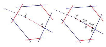
Figure 2.1. Attaching a small A-arc and a B-arc at the point $w$.

Now, given an extended bridge diagram $\mathcal{E}$ which represents a knot in $S^{3}$, we have a following commutative diagram of extended bridge diagrams, where the vertical arrows are stabilizations of type II and horizontal arroLews are either isotopies, handleslides of type I, II, III, IV, stabilizations of type I, or special stabilizations, and $\mathcal{P}(\mathcal{E}_{n})$ (and also $\mathcal{P}(\mathcal{E}_{n}^{st})$) are simple.

Translating this diagram into equivariant Floer cohomology and maps between them gives the following diagram.

All horizontal arrows are isomorphisms. We also know that the leftmost vertical arrow is also an isomorphism, since $\mathcal{P}(\mathcal{E})$ is simple. So, if this diagram is commutative, we can deduce that the map $\widehat{HF}_{\mathbb{Z}_{2}}(\mathcal{E}^{st})\rightarrow\widehat{HF}_{\mathbb{Z}_{2}}(\mathcal{E}),$ which is the map induced by a stabilization of type II applied to $\mathcal{E}$, is an isomorphism.

Lemma 2.19.

Let $(\tilde{\Sigma},\tilde{\boldsymbol{\alpha}},\tilde{\boldsymbol{\beta}},\tilde{\boldsymbol{\gamma}},\tilde{\boldsymbol{\delta}},z)$ be an involutive Heegaard 6-tuple with base $(\Sigma,\boldsymbol{\alpha},\boldsymbol{\beta},\boldsymbol{\gamma},\boldsymbol{\delta},z)$, and $\theta_{\beta,\gamma},\theta_{\gamma,\delta}$ be $\mathbb{Z}_{2}$-invariant cycles in $\widehat{CF}(\tilde{\Sigma},\tilde{\boldsymbol{\beta}},\tilde{\boldsymbol{\gamma}},z),\widehat{CF}(\tilde{\Sigma},\tilde{\boldsymbol{\gamma}},\tilde{\boldsymbol{\delta}},z)$, respectively. Suppose that, for any Floer generator $\mathbf{x}$ of $(\tilde{\Sigma},\tilde{\boldsymbol{\beta}},\tilde{\boldsymbol{\delta}},z)$, every element of $\pi_{2}(\theta_{\beta,\gamma},\theta_{\gamma,\delta},\mathbf{x})$ has Maslov index at least $0$ and achieves transversality for generic $\mathbb{Z}_{2}$-equivariant families of almost complex structures. Then, for any $x_{\alpha,\beta}\in H_{\ast}(\widetilde{CF}_{\mathbb{Z}_{2}}(\tilde{\Sigma},\tilde{\boldsymbol{\alpha}},\tilde{\boldsymbol{\beta}})\otimes_{\mathbb{F}_{2}[\mathbb{Z}_{2}]}\mathbb{F}_{2})$, we have

$$\hat{f}_{\alpha,\gamma,\delta}(\hat{f}_{\alpha,\beta,\gamma}(x_{\alpha,\beta}\otimes\theta_{\beta,\gamma})\otimes\theta_{\gamma,\delta})=\hat{f}_{\alpha,\beta,\delta}(x_{\alpha,\beta}\otimes f_{\beta,\gamma,\delta}(\theta_{\beta,\gamma}\otimes\theta_{\gamma,\delta})),$$

where $\hat{f}$ denotes the equivariant triangle maps, defined in [HLS], and $f$ denotes the ordinary triangle map, with repsect to their subindices.

Proof.

By assumption, the cycle $f_{\beta,\gamma,\delta}(\theta_{\beta,\gamma}\otimes\theta_{\gamma,\delta})\in\widehat{CF}_{\mathbb{Z}_{2}}(\tilde{\Sigma},\tilde{\boldsymbol{\beta}},\tilde{\boldsymbol{\delta}},z)$ is $\mathbb{Z}_{2}$-invariant, so that the term

$$\hat{f}_{\alpha,\beta,\delta}(x_{\alpha,\beta}\otimes f_{\beta,\gamma,\delta}(\theta_{\beta,\gamma}\otimes\theta_{\gamma,\delta}))$$

is well-defined. Using square maps from non-equivariant Floer theory, we can construct the equivariant square map

$$\hat{s}_{\alpha,\beta,\gamma,\delta}\,:\,\widetilde{CF}_{\mathbb{Z}_{2}}(\tilde{\Sigma},\tilde{\boldsymbol{\alpha}},\tilde{\boldsymbol{\beta}},z)\rightarrow\widetilde{CF}_{\mathbb{Z}_{2}}(\tilde{\Sigma},\tilde{\boldsymbol{\alpha}},\tilde{\boldsymbol{\delta}},z),$$

by mimicing the consruction of equivariant triangle maps, as in the proof of Lemma 3.25 in [HLS]. If a sequence of holomorphic squares in $(\tilde{\Sigma},\tilde{\boldsymbol{\alpha}},\tilde{\boldsymbol{\beta}},\tilde{\boldsymbol{\gamma}},\tilde{\boldsymbol{\delta}},z)$ having $\theta_{\beta,\gamma},\theta_{\gamma,\delta}$ as two of their vertices degenerates to a concatenation of a holomorphic triangle in $(\tilde{\Sigma},\tilde{\boldsymbol{\alpha}},\tilde{\boldsymbol{\beta}},\tilde{\boldsymbol{\delta}},z)$ and another holomorphc triangle in $(\tilde{\Sigma},\tilde{\boldsymbol{\beta}},\tilde{\boldsymbol{\gamma}},\tilde{\boldsymbol{\delta}},z)$, the singular vertex should be the points in the cycle $f_{\beta,\gamma,\delta}(\theta_{\beta,\gamma}\otimes\theta_{\gamma,\delta})$ by assumption. Hence, if we choose a cycle representative $\mathbf{x}_{\alpha,\beta}$ of $x_{\alpha,\beta}$, the quantity

$$\hat{f}_{\alpha,\gamma,\delta}(\hat{f}_{\alpha,\beta,\gamma}(\mathbf{x}_{\alpha,\beta}\otimes\theta_{\beta,\gamma})\otimes\theta_{\gamma,\delta})+\hat{f}_{\alpha,\beta,\delta}(\mathbf{x}_{\alpha,\beta}\otimes f_{\beta,\gamma,\delta}(\theta_{\beta,\gamma}\otimes\theta_{\gamma,\delta}))$$

should be the same as the quantity

$$d\hat{s}_{\alpha,\beta,\gamma,\delta}(\mathbf{x}_{\alpha,\beta}\otimes\theta_{\beta,\gamma}\otimes\theta_{\gamma,\delta})+\hat{s}_{\alpha,\beta,\gamma,\delta}(d\mathbf{x}_{\alpha,\beta}\otimes\theta_{\beta,\gamma}\otimes\theta_{\gamma,\delta}).$$

Therefore, by passing to the homology, we get the desired result. ∎

Lemma 2.20.

The maps induced by extended Heegaard moves, and special stabilizations commute with the maps induced by stabilizations of type II.

Proof.

The statement is obvious for diffeomorphisms and special stabilizations. Also, the statement for isotopy maps is a direct consequence of Lemma 6.2 of [K]. The remaining cases involve associativity of equivariant triangle maps, and thus we would like to use Lemma 2.19.

Here, we will only give a proof for the commutation of stabilization maps of type II with handleslides of type IV, since other cases can be proven using the same argument. To give a proof for this case, we consider the two triple-diagram in Figure 2.2. In (the branched double cover of) the given triple-diagrams, there are clearly no nonconstant triangles, and the constant triangles have Maslov index $0$. Also, the induced (non-equivariant) triangle maps sends the top classes to the unique $\mathbb{Z}_{2}$-invariant top class. Therefore, by Lemma 2.19, the maps induced by extended Heegaard moves and special stabilizations commute with the maps induced by stabilizations of type II. ∎

Figure 2.2. The diagram on the left is the triple-diagram for the case when a stabilization map of type II is composed first and then a handleslide map of type IV is composed, and the diagram on the right is for the case when the maps are composed in the opposite order.

Theorem 2.21.

Given an extended bridge diagram $\mathcal{E}$ which represents a knot in $S^{3}$, let $\mathcal{E}^{\prime}$ be the extended bridge diagram we get by applying an extended Heegaard move to $\mathcal{E}$. Suppose that both $\mathcal{E}$ and $\mathcal{E}^{\prime}$ have at least one A-arcs and B-arcs. Then the associated map $\widehat{HF}_{\mathbb{Z}_{2}}(\mathcal{E}^{\prime})\rightarrow\widehat{HF}_{\mathbb{Z}_{2}}(\mathcal{E})$ is an isomorphism.

Proof.

We only have to consider the case when $\mathcal{E}^{\prime}$ is obtained from $\mathcal{E}$ by a stabilization of type II. In this case, recall that we had the following diagram.

We know from Lemma 2.20 that this diagram is commutative. Therefore all vertical arrows should be isomorphisms. In particular, the map $\widehat{HF}_{\mathbb{Z}_{2}}(\mathcal{E}^{\prime})\rightarrow\widehat{HF}_{\mathbb{Z}_{2}}(\mathcal{E})$, induced by a stabilization of type II, is an isomorphism. ∎

Corollary 2.22.

Let $\mathcal{E}$ be an extended bridge diagrams representing a knot in $S^{3}$, which has at least two A-arcs. Then $\widehat{HF}_{\mathbb{Z}_{2}}(\mathcal{E})\simeq\widehat{HF}_{\mathbb{Z}_{2}}(\Sigma(K))$.

Proof.

This follows directly from Theorem 2.21 and Proposition 2.7. ∎

3. Equivariant Heegaard Floer cohomology for knots is a strong Heegaard invariant

Given a based knot $(K,z)$ in $S^{3}$, choose a knot Heegaard diagram $H=(\Sigma,\boldsymbol{\alpha},\boldsymbol{\beta},z,w)$, so that one of the two basepoints of $H$ (which is $z$ here) is the basepoint of the given based knot. By distinguishing the two basepoints $z$ and $w$, we may say that $\mathcal{H}$ represents the based knot $(K,z)$.

Definition 3.1.

We say that a knot Heegaard diagram $H=(\Sigma,\boldsymbol{\alpha},\boldsymbol{\beta},z,w)$ represents a based knot $(K,p)$ in $S^{3}$ if $H$ repesents $K$ and $z=p$. Here, we call $w$ as the second basepoint.

Given such a diagram $H$, we can construct an element $w\in H^{2}(\Sigma\backslash\{z,w\};\mathbb{F}_{2})$ by the following formula.

$$w([\alpha_{i}])=w([\beta_{j}])=0 \text{ for each }\alpha_{i}\in\boldsymbol{\alpha}\text{ and }\beta\in\boldsymbol{\beta}$$

$$w([c])=1 \text{ where }c\text{ is a small circle around }z$$

Since $(\Sigma,\boldsymbol{\alpha},\boldsymbol{\beta},z)$ represents $S^{3}$, the homology classes $[\alpha_{i}]$ and $[\beta_{j}]$ span $H_{2}(\Sigma\backslash\{z,w\};\mathbb{F}_{2})$, so the above formula defines $w$ uniquely. The element $w$ defines a map $\pi_{1}(\Sigma\backslash\{z-w\})\rightarrow\mathbb{Z}_{2}$, thus induces a branched double covering $\tilde{\Sigma}\xrightarrow{f}\Sigma$, branched along $\{z,w\}$. Denote the sets of inverse images of alpha-curves and beta-curves by $\tilde{\boldsymbol{\alpha}}$ and $\tilde{\boldsymbol{\beta}}$. Also, add a small A-arc $a$ and a B-arc $b$ at $w$, as drawn in Figure 3.1. Then the Heegaard diagram $\tilde{H}=((\tilde{\Sigma},\tilde{\boldsymbol{\alpha}},\tilde{\boldsymbol{\beta}}),(\{z,w\},\{a\},\{b\},z))$ is a Heegaard diagram of $\Sigma(K)$ with a $\mathbb{Z}_{2}$-action.

Since $H$ can also be regarded as a 1-bridge knot diagram of $K$ with a hidden pair of bridges $a^{\prime}$ and $b^{\prime}$ connected to $z$, the pair $\mathcal{E}_{H}=((\tilde{\Sigma},\tilde{\boldsymbol{\alpha}},\tilde{\boldsymbol{\beta}}),(\{z,w\},\{a,a^{\prime}\},\{b,b^{\prime}\},z))$ is an extended bridge diagram representing $K$. By the definition of $\widehat{HF}_{\mathbb{Z}_{2}}(\mathcal{E}_{H})$, we have

$$\widehat{HF}_{\mathbb{Z}_{2}}(\mathcal{E}_{H})\simeq\widehat{HF}_{\mathbb{Z}_{2}}(\mathcal{H}_{d}(\tilde{H})).$$

Together with Corollary 2.22, this gives a way to compute the equivariant Heegaard Floer cohomology of a knot from its knot Heegaard Floer cohomology.

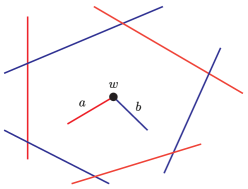
Figure 3.1. Attaching a small A-arc and a B-arc at the point $w$.

Lemma 3.2.

Let $H$ be a knot Heegaard diagram of a based knot $(K,z)$ in $S^{3}$. Then $\widehat{HF}_{\mathbb{Z}_{2}}(\Sigma(K),z)\simeq\widehat{HF}_{\mathbb{Z}_{2}}(\tilde{H})$.

Proof.

By Corollary 2.22, we have $\widehat{HF}_{\mathbb{Z}_{2}}(\Sigma(K),z)\simeq\widehat{HF}_{\mathbb{Z}_{2}}(\mathcal{E}_{H})\simeq\widehat{HF}_{\mathbb{Z}_{2}}(\tilde{H})$. ∎

Recall that any two knot Heegaard diagrams of a given based knot are related by a sequence of Heegaard moves, namely, isotopies, handleslides, (de)stabilizations, and diffeomorphisms. We claim that these basic moves induce isomorphisms of $\widehat{HF}_{\mathbb{Z}_{2}}$, thereby proving that the equivariant Heegaard Floer cohomology is a weak Heegaard invariant.

Theorem 3.3.

Let $H,H^{\prime}$ be two knot Heegaard diagrams of a based knot $(K,z)$, related by a Heegaard move. Then there exists an induced isomorphism

$$\hat{f}_{\mathcal{H}\rightarrow\mathcal{H}^{\prime}}^{basic}\,:\,\widehat{HF}_{\mathbb{Z}_{2}}(\tilde{H})\rightarrow\widehat{HF}_{\mathbb{Z}_{2}}(\tilde{H}^{\prime}).$$

Proof.

The isotopy case is obvious, and the handleslide case follows directly from Proposition 3.24 of [HLS], which proves the invariance of equivariant Floer cohomology under equivariant Hamiltonian isotopies of Lagrangians. The stabilization case is just an application of the standard neck-stretching argument, after assuming that it happens near the basepoint.

It remains to show the case when the given Heegaard move is a diffeomorphism. A diffeomorphism between (knot) Heegaard diagrams has two possible lifts to diffeomorphisms between the branched double covers, and the two lifts differ by the $\mathbb{Z}_{2}$-action. But the $\mathbb{Z}_{2}$-action on $\tilde{H}$ induces the $\mathbb{F}_{2}[\mathbb{Z}_{2}]$-module structure on the freed Floer complex, which is then dualized and tensored with $\mathbb{F}_{2}$ with the trivial $\mathbb{Z}_{2}$-action when calculating the cochain complex $\widehat{CF}_{\mathbb{Z}_{2}}^{\ast}(\tilde{H})$, so that the $\mathbb{Z}_{2}$-action induced on $\widehat{HF}_{\mathbb{Z}_{2}}(\tilde{H})$ is trivial. Therefore the map between $\widehat{HF}_{\mathbb{Z}_{2}}(\tilde{H})$ induced by a diffeomorphism is well-defined. ∎

Corollary 3.4.

The $\mathbb{Z}_{2}$-equivariant Heegaard Floer cohomology of based knots in $S^{3}$ is a weak Heegaard invariant in the sense of Juhasz; see [JT] for the definition of Heegaard invariants.

Proof.

The statement of Theorem 3.3 is precisely the definition of a weak Heegaard invariant. ∎

Remark.

Note that, due to the construction of stabilization maps of type I, we do not know at this stage whether such maps are defined uniquely. This problem will be resolved later.

Now we will show that the $\mathbb{Z}_{2}$-equivariant Heegaard Floer cohomology is not only a weak invariant, but also a strong Heegaard invariant. To recall the definition of strong Heegaard invariants, we consider the graph $\mathcal{G}=\mathcal{G}(K,z)$, for a given based knot $(K,z)$ in $S^{3}$, defined as follows.

$$V(\mathcal{G})= \text{knot Heegaard isotopy diagrams representing }(K,z)$$

$$E(\mathcal{G})=E( \mathcal{G}_{\alpha})\cup E(\mathcal{G}_{\beta})\cup E(\mathcal{G}_{\text{stab}})\cup E(\mathcal{G}_{\text{diff}})$$

Here, isotopy diagram means a diagram in which $\alpha$- and $\beta$-curves are determined up to isotopy, and the graphs $\mathcal{G}_{\alpha},\mathcal{G}_{\beta},\mathcal{G}_{\text{stab}},\mathcal{G}_{\text{diff}}$ are graphs with the same vertex set as $\mathcal{G}$, defined in the following way. $\mathcal{G}_{\alpha}$ is the graph such that for each pair of elements $H_{1},H_{2}\in V(\mathcal{G})$, $\mathcal{G}_{\alpha}(H_{1},H_{2})$ consists of single element if $H_{1},H_{2}$ are $\alpha$-equivalent, i.e. related by a sequence of $\alpha$-equivalences, and is empty otherwise. $\mathcal{G}_{\beta}$ is the defined in the same way, using $\beta$-equivalences. The subgraph $\mathcal{G}_{\text{stab}}$ is the graph of stabilizations, and $\mathcal{G}_{\text{diff}}$ is the graph of diffeomorphisms.

Also, there is a set $\mathcal{D}_{\mathcal{G}}$ of certain subgraphs of $\mathcal{G}$, called distinguished rectangles, defined in Definition 2.30 of [JT]. Then we have the following definition.

Definition 3.5.

(Definition 2.33 of [JT]) A weak Heegaard invariant $F$ (of knots in $S^{3}$) is a strong Heegaard invariant if the following axioms hold.

• (Functoriality) The restriction of $F$ to $\mathcal{G}_{\alpha},\mathcal{G}_{\beta},\mathcal{G}_{\text{diff}}$ are functors, and for any stabilization $e$ and its reverse destabilization $e^{\prime}$, we have $F(e^{\prime})=F(e)^{-1}$.

• (Commutativity) For any distinguished rectangle $D\in\mathcal{D}_{\mathcal{G}}$, the diagram $F(D)$ is commutative.

• (Continuity) If $e$ is a loop-edge of $\mathcal{G}$ which is a diffeomorphism isotopic to the identity, then $F(e)$ is the identity.

• (Handleswap invariance) For every simple handleswap (see Figure 4 in [JT] for its definition)

  in $\mathcal{G}$, we have $F(g)\circ F(f)\circ F(e)=\text{id}$.

For the definition of distinguished rectangles and handleswaps, see section 2.4 of [JT].

Lemma 3.6.

Let $(\tilde{\Sigma},\tilde{\boldsymbol{\alpha}},\tilde{\boldsymbol{\beta}},\tilde{\boldsymbol{\gamma}},\tilde{\boldsymbol{\delta}},z)$ be an involutive Heegaard 6-tuple with base $(\Sigma,\boldsymbol{\alpha},\boldsymbol{\beta},\boldsymbol{\gamma},\boldsymbol{\delta},z)$, and $\theta_{\alpha,\beta},\theta_{\gamma,\delta}$ be $\mathbb{Z}_{2}$-invariant cycles in $\widehat{CF}(\tilde{\Sigma},\tilde{\boldsymbol{\alpha}},\tilde{\boldsymbol{\beta}},z),\widehat{CF}(\tilde{\Sigma},\tilde{\boldsymbol{\gamma}},\tilde{\boldsymbol{\delta}},z)$, respectively. Then, for any $x_{\beta,\gamma}\in H_{\ast}(\widetilde{CF}_{\mathbb{Z}_{2}}(\tilde{\Sigma},\tilde{\boldsymbol{\beta}},\tilde{\boldsymbol{\gamma}})\otimes_{\mathbb{F}_{2}[\mathbb{Z}_{2}]}\mathbb{F}_{2})$, we have

$$\hat{f}_{\alpha,\gamma,\delta}(\hat{f}_{\alpha,\beta,\gamma}(\theta_{\alpha,\beta}\otimes x_{\beta,\gamma})\otimes\theta_{\gamma,\delta})=\hat{f}_{\alpha,\beta,\delta}(\theta_{\alpha,\beta}\otimes f_{\beta,\gamma,\delta}(x_{\beta,\gamma}\otimes\theta_{\gamma,\delta})),$$

where $\hat{f}$ denotes the equivariant triangle maps, defined in [HLS], and $f$ denotes the ordinary triangle map, with repsect to their subindices.

Proof.

The proof is basically the same as in Lemma 2.19, except that we do not need additional condition on triangles. ∎

Lemma 3.7.

Consider a following commutative diagram $\mathcal{D}$ of extended bridge diagram of a based knot in $S^{3}$.

Suppose that $e,e^{\prime}$ are $\alpha$- or A-equivalences and $f,f^{\prime}$ are $\beta$- or B-equivalences. Then $\widehat{HF}_{\mathbb{Z}_{2}}(\mathcal{D})$ commutes, i.e.

$$\widehat{HF}_{\mathbb{Z}_{2}}(e)\circ\widehat{HF}_{\mathbb{Z}_{2}}(f^{\prime})=\widehat{HF}_{\mathbb{Z}_{2}}(f)\circ\widehat{HF}_{\mathbb{Z}_{2}}(e^{\prime}).$$

Proof.

This is a direct application of Lemma 3.6. ∎

Lemma 3.8.

The restriction of the weak Heegaard invariant $\widehat{HF}_{\mathbb{Z}_{2}}$ to $\mathcal{G}_{\alpha}$ is a functor.

Proof.

In this proof, we will use knot bridge diagrams of nontrivial genera and their $\widehat{HF}_{\mathbb{Z}_{2}}$. The idea is to use the naturality of $\widehat{HF}_{\mathbb{Z}_{2}}$ for bridge diagrams on a sphere, which is already established by the author in [K].

Let $\{f_{i}\,:\,H_{i}\rightarrow H_{i+1}\,|\,i=1,\cdots,n\}$ be a composable sequence of $\alpha$-equivalences of knot Heegaard diagrams of a based knot $(K,z)$ in $S^{3}$. Each $f_{i}$ is either an isotopy of $\alpha$-curves or an $\alpha$-handleslide, which can be translated to a 1-parameter family of Morse-Smale pairs on $S^{3}$, as in Proposition 6.35 of [JT]. Composing them gives a 1-parameter family $(f_{t},v_{t})_{t\in[0,1]}$ of simple pairs, where $(f_{t},v_{t})$ is Morse-Smale except for finitely many $t$. Also, there exists a Heegaard surface $\Sigma\subset S^{3}$ which intersects transversely with $K$, contains the basepoint $z$, and is shared by every $(f_{t},v_{t})$, since no stabilizations or destabilizations occur.

Given such a family and a Heegaard surface $\Sigma$, we now choose an isotopy $\{K_{t}\}_{t\in[0,1]}$ of the given based knot $(K,z)$ while fixing the basepoint $z$, such that $K_{0}=K$, $K_{1}$ is an isotopic copy of $K$ which is contained in a very small neighborhood of $z$ and intersects transversely with $\Sigma$. We can further assume that the given isotopy $\{K_{t}\}$ is generic, so that $K_{t}$ is transverse to $\Sigma$ for all but finitely many $t$. Since codimension-1 singularities of $\{K_{t}\}$ correspond to simple tangencies, we know that, when passing through those “finitely many” $t$, a pair of intersection points in $K_{t}\cap\Sigma$ is either created or annihilated.

Now we multiply the two 1-parameter families mentioned above to get a smooth 2-parameter family $\mathcal{F}$;

$$\mathcal{F}=\{(f_{t},v_{t},K_{s})\}_{(t,s)\in[0,1]\times[0,1]}.$$

We can then perturb $\mathcal{F}$ in the space

$$\mathcal{S}=\{\text{simple pairs in }S^{3}\}\times\{\text{knots in }S^{3},\text{ isotopic to }K\text{ and containing }z\}$$

to another generic 2-parameter family $\mathcal{F}^{\prime}$ close to $\mathcal{F}$ in $\mathcal{S}$, which would have finitely many codimension-2 singularities and no higher singularity. But since both $(f_{t},v_{t})$ and $\{K_{s}\}$ were generic, by taking the perturbation to be sufficiently small, we may assume that every codimension-2 singularity arising in $\mathcal{F}^{\prime}$ is a combination of a codimension-1 singularity in the space of simple pairs in $S^{3}$ and a codimension-1 singularity in the space of based knots in $S^{3}$. Furthermore, by closeness, no stabilization/destabilization would occur as a codimension-1 singularity. Therefore we only have to consider the following two possible types of codimension-2 singularities in $\mathcal{S}$.

1. An $\alpha$-handleslide occurs and $K_{s}$ is (simple) tangent to $\Sigma$; $K_{s}$ is transverse to all stable/unstable manifolds of $v_{t}$.

2. An $\alpha$-handleslide occurs and $K_{s}$ intersects transversely with the unstable manifold of a order 1 singularity of $v_{t}$ or the stable manifold of an order 2 singularity of $v_{t}$.

3. An $\alpha$-handleslide occurs and $K_{s}$ is tangent to the stable manifold of a order 1 singularity of $v_{t}$ or the unstable manifold of an order 2 singularity of $v_{t}$.

4. An $\alpha$-handleslide occurs, $K_{s}$ is transverse to $\Sigma$ and all stable/unstable manifolds of $v_{t}$, and the projection of $K_{s}$ to $\Sigma$ via the flow of $v_{t}$ has a simple tangency.

The monodromies of those singularities can be translated as shown below. Note that, in the case 1, we have replaced stabilizations of type II by special stabilizations, as a stabilization of type II can be seen as the composition of a special stabilization followed by a sequence of handleslides of type II, IV, and (A/$\alpha$)-isotopies.

1. Commutation of $\alpha$-handleslides with stabilizations of type II

2. Commutation of $\alpha$-handleslides with handleslides of type II

3. Commutation of $\alpha$-handleslides with compositions of stabilizations of type II and handleslides of type III

4. Commutation of $\alpha$-handleslides with compositions of stabilizations of type II and handleslides of type IV

For a type 2 monodromy, Lemma 2.19 can be used to prove its commutativity, as in the proof of Lemma 2.20. The type 1 monodromy is clearly commutative from the construction of maps associated to special stabilizations, which was given in the proof of Lemma 2.18. A similar argument can be applied to monodromies of type 3 or 4.

It remains to show that $\alpha$-handleslide maps and isotopy maps commute with isotopy maps, which correspond to the regions of $\mathcal{F}^{\prime}$ which does not contain codimension-2 singularity, which can actually be proven by a direct application of the proof of Lemma 6.2 in [K]. Therefore, as in proof of naturality in [K], we have shown that the diagram in Table 3.1 commutes after applying $\widehat{HF}_{\mathbb{Z}_{2}}$, where $\mathcal{E}_{i}^{j}$ are extended bridge diagrams and arrows are extended Heegaard moves. Note that leftmost column and the rightmost column must be identical, i.e. $\mathcal{E}_{1}^{i}=\mathcal{E}_{n}^{i}$ for all $i=1,\cdots,k$, and the extended bridge diagrams $\mathcal{E}_{1}^{k},\cdots,\mathcal{E}_{n}^{k}$ in the bottom row satisfy the property that all A-arcs and B-arcs are contained in the region, bounded by $\alpha$-curves and $\beta$-curves, which contains the basepoint. Also, the handleslides among the arrows in the bottom row can only be handleslides of type I.

Since the extended bridge diagrams appearing in the top row are of the form $\mathcal{B}\sharp\mathcal{H}$ for a genus 0 bridge diagram $\mathcal{B}$ and a (weakly admissible) Heegaard diagram $\mathcal{H}$, where the connected sum is taken near the basepoint $z$ of $\mathcal{H}$, they clearly achieve hypothesis (EH-2) in [HLS], they satisfy equivariant transversality, so that we have a natural isomorphism

$$\widehat{HF}_{\mathbb{Z}_{2}}(\mathcal{B}\sharp\mathcal{H})\simeq\widehat{HF}_{\mathbb{Z}_{2}}(\mathcal{B})\otimes_{\mathbb{F}_{2}}\widehat{HF}(\mathcal{H})\simeq\widehat{HF}_{\mathbb{Z}_{2}}(\mathcal{B}),$$

since $\mathcal{H}$ represents $S^{3}$ and so $\widehat{HF}(\mathcal{H})\simeq\mathbb{F}_{2}$. Thus, by the naturality of $\widehat{HF}_{\mathbb{Z}_{2}}$ for genus-0 bridge diagrams of based knots in $S^{3}$, we deduce that the composition

$$\widehat{HF}_{\mathbb{Z}_{2}}(f_{1})\circ\cdots\circ\widehat{HF}_{\mathbb{Z}_{2}}(f_{n})\,:\,\widehat{HF}_{\mathbb{Z}_{2}}(H_{n})\rightarrow\widehat{HF}_{\mathbb{Z}_{2}}(H_{1})$$

does not depend on the choice of a sequence $f_{1,}\cdots,f_{n}$. Therefore the restriction of $\widehat{HF}_{\mathbb{Z}_{2}}$ to $\mathcal{G}_{\alpha}$ is a functor. ∎

Table 3.1. A diagram of extended bridge diagrams and extended Heegaard moves, which becomes commutative after taking $\widehat{HF}_{\mathbb{Z}_{2}}$. What we have actually shown is that the interior of this diagram can be filled with smaller diagrams which represent monodromies around the singularities of $\mathcal{F}^{\prime}$, and such diagrams are commutative after taking $\widehat{HF}_{\mathbb{Z}_{2}}$.

Remark 3.9.

The proof of Lemma 3.8 can be directly extended to extended bridge diagrams representing based knots in $S^{3}$ to show that any loop consisting of A-equivalences and $\alpha$-equivalences induce the identity map in $\widehat{HF}_{\mathbb{Z}_{2}}$. Furthermore, applying 3.7 gives us that any loop of basic moves induce the identity map in $\widehat{HF}_{\mathbb{Z}_{2}}$.

Proposition 3.10.

Let $\mathcal{E}_{1},\mathcal{E}_{2}$ be extended bridge diagrams of a based knot $(K,z)$ in $S^{3}$, related by a single stabilization (of type I or II), and let $\mathcal{E}_{1}\xrightarrow{s}\mathcal{E}_{2}$ be such a stabilization. Then the induced map

$$\widehat{HF}_{\mathbb{Z}_{2}}(s)\,:\,\widehat{HF}_{\mathbb{Z}_{2}}(\mathcal{E}_{2})\rightarrow\widehat{HF}(\mathcal{E}_{1})$$

is defined uniquely.

Proof.

Since the proof of type I and II are similar, we will only work out the case of type I explicitly. Let $\Sigma$ be the Heegaard surface of $\mathcal{H}_{\text{pt}}(\mathcal{E}_{1})$ and choose a point $w$ which is very close to the basepoint $z$. Let $\mathcal{E}$ be the extended bridge diagram given by performing a stabilization of type I on $\mathcal{E}_{1}$ at $w$; write the induced map as

$$\widehat{HF}_{\mathbb{Z}_{2}}(s_{w})\,:\,\widehat{HF}_{\mathbb{Z}_{2}}(\mathcal{E})\rightarrow\widehat{HF}_{\mathbb{Z}_{2}}(\mathcal{E}_{1}).$$

Recall that, to construct an induced map for a stabilization of type I performed at another point on $\Sigma$, which is not near $z$, we have to compose $\widehat{HF}_{\mathbb{Z}_{2}}(s_{w})$ with maps induced by $\alpha$- and $\beta$-handleslides. To prove that $\widehat{HF}_{\mathbb{Z}_{2}}(s)$ is unique, we have to prove that for any sequence of $\alpha$-handleslides which starts from and ends at $\mathcal{E}$, the induced automorphism of $\widehat{HF}_{\mathbb{Z}_{2}}(\mathcal{E})$ is the identity. But this is a direct consequence of Lemma 3.11. Therefore $\widehat{HF}_{\mathbb{Z}_{2}}(s)$ is uniquely defined. ∎

With the fact that the maps induced by stabilizations are uniquely defined, we can now finish the proof of functoriality condition.

Lemma 3.11.

The weak Heegaard invariant $\widehat{HF}_{\mathbb{Z}_{2}}$ satisfies functoriality condition of Definition 3.5.

Proof.

By Lemma 3.8, we know that the restriction of $\widehat{HF}_{\mathbb{Z}_{2}}$ to $\mathcal{G}_{\alpha}$ is a functor. So, by the same argument applied to $\beta$-curves instead of $\alpha$-curves, we also see that the restriction of $\widehat{HF}_{\mathbb{Z}_{2}}$ to $\mathcal{G}_{\beta}$ is also a functor. If $e$ is a stabilization and $e^{\prime}$ is its reverse, we can apply Proposition 3.10 to reduce to the case when the (de)stabilization is performed near the basepoint, in which case $\widehat{HF}_{\mathbb{Z}_{2}}(e)\circ\widehat{HF}_{\mathbb{Z}_{2}}(e^{\prime})=\text{id}$ holds by choosing a suitable family of almost complex structures. The diffeomorphism part is obvious. ∎

We now move on to a proof of continuity condition.

Lemma 3.12.

The weak Heegaard invariant $\widehat{HF}_{\mathbb{Z}_{2}}$ satisfies continuity condition of Definition 3.5.

Proof.

We will prove a slightly more general statement, that for any weakly admissible extended bridge diagram $\mathcal{E}$ of a based knot $(K,z)$ in $S^{3}$ and a self-diffeomorphism $\phi$ of $\mathcal{E}$ which is isotopic to the identity, the map

$$\widehat{HF}_{\mathbb{Z}_{2}}(\phi)\in\text{Aut}_{\mathbb{F}_{2}[\theta]}(\widehat{HF}_{\mathbb{Z}_{2}}(\Sigma(K),z))$$

induced by $\phi$ is the identity.

If $\mathcal{E}$ is a bridge diagram on a sphere, then by the genus-0 naturality of $\widehat{HF}_{\mathbb{Z}_{2}}$, we know that $\widehat{HF}_{\mathbb{Z}_{2}}(\phi)=\text{id}$. Next, suppose that $\mathcal{E}$ satisfies the following property.

• There exists a small disk $D$ on the Heegaard surface $\Sigma$ of $\mathcal{H}_{\text{pt}}(\mathcal{E})$, near its basepoint $z$, so that all A- and B-arcs of $\mathcal{H}_{\text{pt}}(\mathcal{E})$ are contained in $D$ and all $\alpha$- and $\beta$-arcs are contained in $\Sigma\backslash D$.

Then we may assume that $\phi$ fixes the curve $\partial D$, and by taking $\partial D$ as the connected-sum neck, we can represent $\mathcal{E}$ as a connected sum:

$$\mathcal{E}=\mathcal{B}\sharp\mathcal{H},$$

where $\mathcal{B}$ is a bridge diagram of $(K,z)$ on a sphere and $\mathcal{H}$ is a Heegaard diagram representing $S^{3}$. As in the proof of 3.8, we have a decomposition

$$\widehat{HF}_{\mathbb{Z}_{2}}(\mathcal{E})\simeq\widehat{HF}_{\mathbb{Z}_{2}}(\mathcal{B})\otimes_{\mathbb{F}_{2}}\widehat{HF}(\mathcal{H},\text{pt})\simeq\widehat{HF}_{\mathbb{Z}_{2}}(\mathcal{B})$$

by stretching the neck to infinite length. By assumption, the action of $\phi$ on $\widehat{HF}_{\mathbb{Z}_{2}}(\mathcal{H})$ reduces to $\widehat{HF}_{\mathbb{Z}_{2}}(\mathcal{B})$. But since $\mathcal{B}$ is a genus-0 diagram, we already know that $\phi$ acts trivially on it. Hence $\widehat{HF}_{\mathbb{Z}_{2}}(\phi)=\text{id}$ in this case.

Finally, we work out the general case. As in the proof of Lemma 3.8, we know that there exists a sequence of extended Heegaard moves, except stabilizations of type I (whose “induced map” is not uniquely defined yet in the general case, in particular, if it occurs in a point not close to the basepoint), from $\mathcal{E}$ to another extended bridge diagram $\mathcal{E}^{\prime}$ which satisfies the above property. Now, by the definition of diffeomorphism map (it just acts by diffeomorphism), we know that it commutes with maps induced by all extended Heegaard moves except stabilizations of type I. Therefore the problem reduces to the former case and we are done. ∎

Now we will prove that the commutativity condition also holds. For that, we recall the definition of distinguished rectangles, defined in Definition 2.30 of [JT].

Definition 3.13.

Let $H_{i}=(\Sigma_{i},[\boldsymbol{\alpha}_{i}],[\boldsymbol{\beta}_{i}])$ be isotopy diagrams for $i=1,\cdots,4$. A distinguished rectangle in $\mathcal{G}$ is a subgraph

of $\mathcal{G}$ that satisfies one of the following properties.

1. Both $e$ and $h$ are $\alpha$-equivalences, while both $f$ and $g$ are $\beta$-equivalences.

2. Both $e$ and $h$ are $\alpha$- or $\beta$-equivalences, while $f$ and $g$ or both stabilizations.

3. Both $e$ and $h$ are $\alpha$- or $\beta$-equivalences, while $f$ and $g$ are both diffeomorphisms. In this case, we necessarily have $\Sigma_{1}=\Sigma_{2}$ and $\Sigma_{3}=\Sigma_{4}$, and we require in addition that the diffeomorphisms $\Sigma_{1}\xrightarrow{f}\Sigma_{3}$ and $\Sigma_{2}\xrightarrow{g}\Sigma_{4}$ are the same.

4. The maps $e,f,g,h$ are all stabilizations, such that there are disjoint disks $D_{1},D_{2}\subset\Sigma_{1}$ and disjoint punctured tori $T_{1},T_{2}\subset\Sigma_{4}$ satisfying $\Sigma_{1}\backslash(D_{1}\cup D_{2})=\Sigma_{4}\backslash(T_{1}\cup T_{2})$, $\Sigma_{2}=(\Sigma_{1}\backslash D_{1})\cup T_{1}$, and $\Sigma_{3}=(\Sigma_{1}\backslash D_{2})\cup T_{2}$.

5. The maps $e,h$ are stabilizations, while $f,g$ are diffeomorphisms. Furthermore, there are disks $D\subset\Sigma_{1}$ and $D^{\prime}\subset\Sigma_{4}$ and punctured tori $T\subset\Sigma_{2}$ and $T^{\prime}\subset\Sigma_{4}$ such that $\Sigma_{1}\backslash D=\Sigma_{2}\backslash T$, $\Sigma_{3}\backslash D^{\prime}=\Sigma_{4}\backslash T^{\prime}$, and the diffeomorphisms $f,g$ satisfy $f(D)=D^{\prime}$, $g(T)=T^{\prime}$, and $f|_{\Sigma_{1}\backslash D}=g|_{\Sigma_{2}\backslash T}$.

Lemma 3.14.

The weak Heegaard invariant $\widehat{HF}_{\mathbb{Z}_{2}}$ satisfies commutativity condition of Definition 3.5.

Proof.

Commutativity for distinguished rectangles of type 1 is proven in Lemma 3.7. For the remaining cases, recall that a stabilization map are defined by composing the map induced by a stabilization near the basepoint following by $\alpha$- and $\beta$-equivalences. Also, given a knot Heegaard diagram $\mathcal{H}$ representing a based knot $(K,z)$ and another diagram $\mathcal{H}^{\prime}$ given by stabilizing $\mathcal{H}$ near $z$, the stabilization map is given explicitly by

$$\widehat{HF}_{\mathbb{Z}_{2}}(\tilde{\mathcal{H}}) \rightarrow\widehat{HF}_{\mathbb{Z}_{2}}(\tilde{\mathcal{H}}^{\prime}),$$

$$\mathbf{x} \mapsto\mathbf{x}\cup p^{-1}(\{c\}),$$

where $p$ is the branched double covering map and $c$ is the new intersection point introduced by the stabilization, by taking family of almost complex structure of the form $\text{Sym}^{g}(\mathfrak{j})$, the reason being that any holomorphic disk involving the Floer generator in $p^{-1}(\{c\})$ must intersect the basepoint. But this argument also works for counting holomorphic triangles, and thus we deduce that the maps induced by $\alpha$- and $\beta$-equivalences and stabilizations must commute, thereby proving commutativity of distinguished rectangles of type 2.

Now, we can apply the functoriality condition, which is already proven in Lemma 3.11, together with commutativity of distinguisehd rectangles of type 2, to reduce the distinguished rectangles of type 3,4,5 to the case when all stabilizations involved are performed near the basepoint. Then, by the above description of maps induced by stabilizations near the basepoint $z$, they must commute with stabilization maps and diffeomorphism maps. Therefore $\widehat{HF}_{\mathbb{Z}_{2}}$ satisfies commutativity for all distinguished rectangles. ∎

Remark 3.15.

The proof of Lemma 3.14 can be directly extended to stabilization of type I on extended bridge diagrams. The result we get is that stabilization maps of type I and diffeomorphism maps commutes with any maps induced by extended Heegaard diagrams.

We will now prove that $\widehat{HF}_{\mathbb{Z}_{2}}$ satisfies handleslide invariance.

Lemma 3.16.

The weak Heegaard invariant $\widehat{HF}_{\mathbb{Z}_{2}}$ satisfies handleswap invariance condition of Definition 3.5.

Proof.

Let $H=H_{0}\sharp H_{s}$ be a knot Heegaard diagram representing a based knot $(K,z)$ in $S^{3}$, where $H_{0}$ is double-pointed, $H_{s}$ is the diagram drawn in Figure 3.2, and suppose that we perform a simple handleswap on $H_{s}$. If the connected sum is taken near $z$, then as in the proof of Lemma 9.30 in [JT], we are done.

In the general case, let $\Sigma_{0}$ and $\Sigma_{s}$ be the Heegaard surfaces of $H_{0}$ and $H_{s}$, respectively, and let $p$ be the point in $\Sigma_{0}$ at which we take the connected sum. Define a subset of $\Sigma_{0}\backslash(\{z\}\cup(\alpha,\beta\text{-curves of }H_{0})$ as follows.

$$X=\{p\in\Sigma_{0}\backslash(\{z\}\cup(\alpha,\beta\text{-curves of }H_{0})\,|\,\text{handleswap invariance holds for }H\}$$

Then, by functoriality(Lemma 3.11) and continuity(Lemma 3.14), we know that $X$ is a union of some connected components.. Also, we already know that the connected component containing $z$ is contained in $X$, so that $X\neq\emptyset$.

Now let $p\in\Sigma_{0}\backslash(\alpha,\beta\text{-curves of }H_{0})$ be a point satisfying the following property.

• Let $R$ be the connected component of $\Sigma_{0}\backslash(\{z\}\cup(\alpha,\beta\text{-curves of }H_{0}))$ containing $p$. Then $\overline{R}\cap X$ contains a segment of either an $\alpha$-curve or a $\beta$-curve.

Then, without loss of generality, we may assume that there exists a point $p^{\prime}\in X$ such that, when we denote the connected sums of $H_{0}$ and $H_{s}$ performed at $p$ and $p^{\prime}$ as $H$ and $H^{\prime}$, respecively, the knot Heegaard diagrams $H$ and $H^{\prime}$ are related by a sequence of four $\alpha$-handleslides. Hence, by Lemma 3.25 of [HLS], the equivariant triangle map

$$F_{H,H^{\prime}}\,:\,\widehat{HF}_{\mathbb{Z}_{2}}(\widetilde{H^{\prime}})\rightarrow\widehat{HF}_{\mathbb{Z}_{2}}(\widetilde{H}),$$

defined using the top class $\mathbf{x}$ drawn in Figure 3.3, is an isomorphism; we will call this map as the $\alpha$-crossing map. We will not prove that the crossing map is the same as the composition of four $\alpha$-handleslide maps, as we do not need it to prove this lemma. Note that, although we are drawing knot Heegaard diagrams, we are actually working with their branched double coverings.

Now consider the simple handleswap diagram involving $H$, and another simple handleswap diagram involving $H^{\prime}$. Taking $\widehat{HF}_{\mathbb{Z}_{2}}$ gives the following diagram, where every edge is an isomorphism. Note that the innermost and the outermost triangle are simple handleswap diagrams and all crossing maps are $\alpha$-crossing maps.

Since diffeomorphism maps clearly commutes with crossing maps, the leftmost face is commutative. Also, by Lemma 3.6, we see that the face in the right-bottom corner is also commutative, and the same argument works for the commutativity of the topmost face.

Now, the central triangle is commutive by assumption. Thus every face of the diagram is commutative. Since all edges of the diagram are isomorphisms, the peripheral triangle must also be commutative. Hence $p\in X$ by the definition of $X$. Therefore, by induction on the number of $\alpha$- and $\beta$-curves needed to cross to travel from $p$ to $z$, we deduce that

$$X=\Sigma_{0}\backslash(\{z\}\cup(\alpha,\beta\text{-curves of }H_{0}),$$

i.e. $\widehat{HF}_{\mathbb{Z}_{2}}$ satisfies handleswap invariance condition of Definition 3.5. ∎

Figure 3.2. The Heegaard diagram $H_{s}$; the boundary is collapsed to form a genus 2 surface.

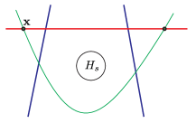
Figure 3.3. The triple-diagram near the connected sum region. The circle in the middle is where the diagram $H_{s}$ is attached via connected sum neck.

Theorem 3.17.

There exists a strong Heegaard invariant of based knots in $S^{3}$, which is isomorphic to $\widehat{HF}_{\mathbb{Z}_{2}}$.

Proof.

By Lemma 3.11, Lemma 3.12, Lemma 3.14, and Lemma 3.16, $\widehat{HF}_{\mathbb{Z}_{2}}$ satisfies all conditions of Definition 3.5. Therefore it is a strong Heegaard invariant. ∎

The important point of Theorem 3.17 is that, instead of treating $\widehat{HF}$ directly as a Heegaard invariant, we have used the word “isomorphic”. The reason is as follows. While it is true that we have constructed a strong Heegaard invariant $\widehat{HF}_{\mathbb{Z}_{2}}(\Sigma(K),z)$ of based knots $(K,z)$ in $S^{3}$, defined using knot Heegaard diagrams,we also have another definition of $\widehat{HF}_{\mathbb{Z}_{2}}(\Sigma(K),z)$ using bridge diagrams of $(K,z)$ on $S^{2}$. Both versions of $\widehat{HF}_{\mathbb{Z}_{2}}$ are natural invariants, i.e. define functors

$$\widehat{HF}_{\mathbb{Z}_{2}}^{knot},\,\widehat{HF}_{\mathbb{Z}_{2}}^{bridge}\,:\,\text{Knot}_{\ast}\rightarrow\text{Mod}_{\mathbb{F}_{2}[\theta]},$$

where $\text{Knot}_{\ast}$ is the category whose objects are based knots in $S^{3}$ and morphisms are diffeomorphisms. Also, Theorem 3.17 tells us that both of the have the same isomorphism type (of $\mathbb{F}_{2}[\theta]$-modules). However, we have not yet proven whether they are isomorphic through a natural isomorphism, i.e. there exists a natural transformation $\eta$ between functors $\widehat{HF}_{\mathbb{Z}_{2}}^{knot}$ and $\widehat{HF}_{\mathbb{Z}_{2}}^{bridge}$.

We will now construct such a natural transformation; note that, while dealing with this issue, we will strictly distinguish the two invariants $\widehat{HF}_{\mathbb{Z}_{2}}^{knot}$ and $\widehat{HF}_{\mathbb{Z}_{2}}^{bridge}$. Let $\mathcal{E}=((\Sigma,\boldsymbol{\alpha},\boldsymbol{\beta}),(P,A,B,z))$ be an extended bridge diagram representing a based knot $(K,z)$ in $S^{3}$. Choose a point $p\in\text{int}(A_{i})\cap\text{int}(B_{j})$ for some $A_{i}\in A$, $B_{j}\in B$, where $z\notin A_{i}\cup B_{j}$; such a point will be called as a proper crossing of $\mathcal{E}$. Let $D\subset\Sigma$ be a small disk neighborhood of $p$, which does not intersect $\alpha$- and $\beta$-curves and intersects A- and B-arcs only with $A_{i}$ and $B_{j}$, satisfying $D\cap(A_{i}\cup B_{j})=\{p\}$. Then, on a puncture torus $T$ whose boundary $\partial T$ is identified with $\partial D$, draw two disjoint simple arcs, denoted $A_{i}^{p}$ and $B_{j}^{p}$, so that $\partial A_{i}^{p}=\partial A_{i}$ and $\partial B_{j}^{p}=\partial B_{j}$. Also, draw two disjoint simple closed curves, denoted $\alpha_{p}$ and $\beta_{p}$, so that the following conditions hold.

• $A_{i}^{p}\cap\alpha_{p}=B_{j}^{p}\cap\beta_{p}=\emptyset$.

• $\alpha_{p}$ intersects $B_{j}^{p}$ transversely at one point.

• $\beta_{p}$ intersects $A_{i}^{p}$ transversely at one point.

Now define the following objects.

• $\Sigma^{p}=(\Sigma\backslash D)\cup T$

• $\boldsymbol{\alpha}^{p}=\boldsymbol{\alpha}\cup\{\alpha_{p}\}$, $\boldsymbol{\beta}^{p}=\boldsymbol{\beta}\cup\{\beta_{p}\}$

• $A^{p}=(A\backslash\{A_{i}\})\cup\{A_{i}^{p}\}$, $B^{p}=(B\backslash\{B_{j}\})\cup\{B_{j}^{p}\}$

Then the pair

$$R_{p}(\mathcal{E})=((\Sigma^{p},\boldsymbol{\alpha}^{p},\boldsymbol{\beta}^{p}),(P,A^{p},B^{p},z))$$

also represents $(K,z)$. Furthermore, $\mathcal{E}$ and $R_{p}(\mathcal{E})$ are related by a sequence consisting of a stabilization of type I and two handleslides of type III. Hence, by taking $\widehat{HF}_{\mathbb{Z}_{2}}$ and composing the induced maps, we get an isomorphism, which we will call as the resolution map at $p$:

$$\mathcal{R}_{p,\mathcal{E}}\,:\,\widehat{HF}_{\mathbb{Z}_{2}}(R_{p}(\mathcal{E}))\rightarrow\widehat{HF}_{\mathbb{Z}_{2}}(\mathcal{E}).$$

Lemma 3.18.

Given an extended bridge diagram $\mathcal{E}$ representing a based knot $(K,z)$ in $S^{3}$, and its proper crossing $p$, the resolution map $\mathcal{R}_{p,\mathcal{E}}$ depends only on the choice of $p$.

Proof.

The definition of $\mathcal{R}_{p,\mathcal{E}}$ involves choosing a point in $D\backslash(A_{i}\cup B_{j})$, at which a stabilization of type I would occur, and also choosing which one of two handleslides of type I/II is to be applied first. Take any two possible choices, and denote the two maps given by taking compositions of the induced maps as $\mathcal{R}_{p,\mathcal{E}}^{1}$ and $\mathcal{R}_{p,\mathcal{E}}^{2}$. Then the composition $(\mathcal{R}_{p,\mathcal{E}}^{2})^{-1}\circ\mathcal{R}_{p,\mathcal{E}}^{1}$, which is an automorphism of $\widehat{HF}_{\mathbb{Z}_{2}}(\Sigma(K),z)$, can be decomposed as

$$(\mathcal{R}_{p,\mathcal{E}}^{2})^{-1}\circ\mathcal{R}_{p,\mathcal{E}}^{1} =(\text{basic moves})\circ(\text{destabilization})\circ(\text{stabilization})\circ(\text{basic moves})$$

$$=(\text{basic moves})\circ(\text{special destab})\circ(\text{special stab})\circ(\text{basic moves})$$

$$=\text{composition of basic moves}$$

where Lemma 3.7 is applied in the first line. Now, by Remark 3.9, this map should be the identity. Therefore $\mathcal{R}_{p,\mathcal{E}}^{1}=\mathcal{R}_{p,\mathcal{E}}^{2}$. ∎

Lemma 3.19.

Let $p,q$ be two distinct proper crossings of $\mathcal{E}$. Then we have

$$\mathcal{R}_{p,\mathcal{E}}\circ\mathcal{R}_{q,R_{p}(\mathcal{E})}=\mathcal{R}_{q,\mathcal{E}}\circ\mathcal{R}_{p,R_{q}(\mathcal{E})}.$$

In other words, resolution maps of distinct proper crossings commute.

Proof.

Using Lemma 3.14 and Remark 3.18, we can see that the map

$$(\mathcal{R}_{p,\mathcal{E}}\circ\mathcal{R}_{q,R_{p}(\mathcal{E})})^{-1}\circ\mathcal{R}_{q,\mathcal{E}}\circ\mathcal{R}_{p,R_{q}(\mathcal{E})}$$

is a composition of maps induced by a loop of basic moves, thus is the identity. ∎

Given an extended bridge diagram $\mathcal{E}$ representing a based knot $(K,z)$ in $S^{3}$, let $\mathcal{I}$ be the set of all proper crossings of $\mathcal{E}$. Choose an enumeration $\mathcal{I}=\{x_{1},\cdots,x_{n}\}$. Define an extended bridge diagram $R(\mathcal{E})$, which depends only on $\mathcal{E}$, as follows.

$$R(\mathcal{E})=R_{x_{n-1}}(\cdots(\mathcal{R}_{x_{1}}(\mathcal{E}))\cdots)$$

Also, define an isomorphism $\mathcal{R}_{\mathcal{E}}\,:\,\widehat{HF}_{\mathbb{Z}_{2}}(R(\mathcal{E}))\rightarrow\widehat{HF}_{\mathbb{Z}_{2}}(\mathcal{E})$ as follows.

$$\mathcal{R}_{\mathcal{E}}=\mathcal{R}_{x_{1},\mathcal{E}}\circ\cdots\circ\mathcal{R}_{x_{n},R_{x_{n-1}}(\cdots(\mathcal{R}_{x_{1}}(\mathcal{E}))\cdots)}$$

Then, by Lemma 3.18 and Lemma 3.19, $\mathcal{R}_{\mathcal{E}}$ does not depend on the choice of an enumeration of $\mathcal{I}$, thus depends only on $\mathcal{E}$.

Now observe that the A- and B-arcs of $R(\mathcal{E})$ which do not contain $z$ also do not intersect themselves in their interior. So, after performing handleslides as in Figure 3.4 on $R(\mathcal{E})$, it can then be destabilized (of type II) to a knot Heegaard diagram $HR(\mathcal{E})$ representing $(K,z)$. Denote the composition of destabilization maps as

$$\mathcal{D}_{\mathcal{E}}\,:\,\widehat{HF}_{\mathbb{Z}_{2}}(\widetilde{HR(\mathcal{E})})\rightarrow\widehat{HF}_{\mathbb{Z}_{2}}(R(\mathcal{E})).$$

Then, by Lemma 2.20, $\mathcal{D}_{\mathcal{E}}$ also depends only on $\mathcal{E}$.

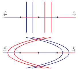
Figure 3.4. The diagrams $R(\mathcal{E})$(above) and $HR(\mathcal{E})$(below) near the A-arcs and B-arcs. Here, we assume for simplicity that the rightmost A-arc and the leftmost B-arc are the ones connected to the basepoint $z$.

Definition 3.20.

Given an extended bridge diagram $\mathcal{E}$ representing a based knot $(K,z)$ in $S^{3}$, we define its translation isomorphism as

$$\mathcal{T}_{\mathcal{E}}=(\mathcal{R}_{\mathcal{E}}\circ\mathcal{D}_{\mathcal{E}})^{-1}\,:\widehat{HF}_{\mathbb{Z}_{2}}(\mathcal{E})\rightarrow\,\widehat{HF}_{\mathbb{Z}_{2}}(\widetilde{HR(\mathcal{E})}).$$

We will now prove that translation isomorphisms define a natural transformation between $\widehat{HF}_{\mathbb{Z}_{2}}^{knot}$ and $\widehat{HF}_{\mathbb{Z}_{2}}^{bridge}$.

Lemma 3.21.

Let $\mathcal{E}\xrightarrow{s}\mathcal{E}^{\prime}$ be an extended Heegaard move between extended bridge diagrams $\mathcal{E},\mathcal{E}^{\prime}$ representing a based knot $(K,z)$ in $S^{3}$.

1. If $s$ is a basic move, then the knot Heeegaard diagrams $HR(\mathcal{E})$ and $HR(\mathcal{E}^{\prime})$ are related by a sequence of basic moves and stabilizations of type I.

2. If $s$ is a stabilization of type I, then $HR(\mathcal{E})$ and $HR(\mathcal{E}^{\prime})$ are also related by a stabilization of type I.

3. If $s$ is a stabilization of type II, then $HR(\mathcal{E})=HR(\mathcal{E}^{\prime})$.

4. If $s$ is a diffeomorphism, then $HR(\mathcal{E})$ and $HR(\mathcal{E}^{\prime})$ are also related by a diffeomorphism.

Proof.

Cases 2, 3, and 4 are obvious. For case 1, it can be easily seen that $R(\mathcal{E})$ and $R(\mathcal{E}^{\prime})$ are related by a sequence of basic moves and stabilizations of type I. Since $HR$ is obtained from $R$ by performing handleslides of type III, we deduce that $HR(\mathcal{E})$ and $HR(\mathcal{E}^{\prime})$ are also related by a sequecne of basic moves and stabilizations of type I. ∎

Theorem 3.22.

Translation isomorphisms define an invertible natural transformation between the functors

$$\widehat{HF}_{\mathbb{Z}_{2}}^{knot},\,\widehat{HF}_{\mathbb{Z}_{2}}^{bridge}\,:\,\text{Knot}_{\ast}\rightarrow\text{Mod}_{\mathbb{F}_{2}[\theta]}.$$

Proof.

Let $\mathcal{B}\xrightarrow{s}\mathcal{B}^{\prime}$ be an extended Heegaard diagram between bridge diagrams $\mathcal{B},\mathcal{B}^{\prime}$ representing a based knot $(K,z)$ in $S^{3}$, and denote the isomorphism induced by $s$ by

$$\widehat{HF}_{\mathbb{Z}_{2}}^{bridge}(s)\,:\,\widehat{HF}_{\mathbb{Z}_{2}}^{bridge}(\mathcal{B}^{\prime})\rightarrow\widehat{HF}_{\mathbb{Z}_{2}}^{bridge}(\mathcal{B}).$$

If $s$ is a basic move or a stabilization, then by Lemma 3.21, there exists either a (possibly empty) sequence of basic moves and stabilizations from $HR(\mathcal{B})$ and $HR(\mathcal{B}^{\prime})$; denote the induced map by

$$\widehat{HF}_{\mathbb{Z}_{2}}^{knot}(HR(s))\,:\,\widehat{HF}_{\mathbb{Z}_{2}}^{bridge}(\widetilde{HR(\mathcal{B}^{\prime})})\rightarrow\widehat{HF}_{\mathbb{Z}_{2}}^{bridge}(\widetilde{HR(\mathcal{B})}).$$

Then $(\widehat{HF}_{\mathbb{Z}_{2}}^{bridge}(s)\circ\mathcal{T}_{\mathcal{B}})^{-1}\circ\mathcal{T}_{\mathcal{B}^{\prime}}\circ\widehat{HF}_{\mathbb{Z}_{2}}^{knot}(HR(s))$ is the map induced by a loop consisting of basic moves and stabilizations. Hence, by Lemma 2.20, Remark 3.15, and Remark 3.9, we see that it is equal to the identity map, i.e.

$$\widehat{HF}_{\mathbb{Z}_{2}}^{bridge}(s)\circ\mathcal{T}_{\mathcal{B}}=\mathcal{T}_{\mathcal{B}^{\prime}}\circ\widehat{HF}_{\mathbb{Z}_{2}}^{knot}(HR(s)).$$

Thus the translation maps induce a well-defined map

$$\mathcal{T}_{(K,z)}\,:\,\widehat{HF}_{\mathbb{Z}_{2}}^{bridge}(\Sigma(K),z)\rightarrow\widehat{HF}_{\mathbb{Z}_{2}}^{knot}(\Sigma(K),z).$$

Now, again by Remark 3.15, we know that $\mathcal{T}_{K}$ commutes with diffeomorphism maps. However the morphisms of the category $\text{Knot}_{\ast}$ are precisely diffeomorphism. Therefore the correspondence

$$\mathcal{T}\,:\,(K,z)\mapsto\mathcal{T}_{(K,z)}$$

is a natural transformation from $\widehat{HF}_{\mathbb{Z}_{2}}^{bridge}$ to $\widehat{HF}_{\mathbb{Z}_{2}}^{knot}$. Since $\mathcal{T}_{(K,z)}$ is an isomorphism for each based knot $(K,z)$ in $S^{3}$, the natural transformation $\mathcal{T}$ is invertible. ∎

4. The $\widehat{HF}_{\mathbb{Z}_{2}}$ of very nice knot Heegaard diagrams

Given a knot $K$ in $S^{3}$, we can combinatorially compute its knot Floer homology $\widehat{HFK}(S^{3},K)$ in the following way. Choose any knot Heegaard diagram $H_{0}$ representing $K$. Theorem 1.2 of [SW] tells us that we can convert $H_{0}$ into a nice diagram $H$ using only isotopies and handleslides. Here, we say that $H$ is nice if the follwing condition holds.

• Every region of $H$ bounded by $\alpha$- and $\beta$-curves, which does not contain basepoints of $H$, is either a bigon or a square.

Then, by Theorem 3.3 and Theorem 3.4 of [SW], for any Floer generators $\mathbf{x}$,$\mathbf{y}$ and a Whitney disk $\phi\in\pi_{2}^{0}(\mathbf{x},\mathbf{y})$ with $\mu(\phi)=1$, there exists a holomorphic representative of $\phi$ if and only if the domain $\mathcal{D}(\phi)$ of $\phi$ is either a bigon or a square which does not contain basepoints of $H$, and the moduli space of holomorphic representatives of $\phi$ is a point. This allows us to describe $\widehat{CFK}(S^{3},K)$ and thus compute $\widehat{HFK}(S^{3},K)$ in a combinatorial way.

We will now prove that we can also compute $\widehat{HF}_{\mathbb{Z}_{2}}(\Sigma(K),z)$ in a combinatorial way, without using desirable bridge diagrams of $K$ as in Figure 1 of [HLS]. The key idea is to use diagrams satisfying the conditions similar to nice diagrams. For the technical terms arising in Lemma 4.2 involving details of the construction of $\mathbb{Z}_{2}$-equivariant Heegaard Floer cohomology, one can find their definitions in section 3 of [HLS].

Definition 4.1.

A knot Heegaard diagram $H=(\Sigma,\boldsymbol{\alpha},\boldsymbol{\beta},z,w)$ representing a based knot $(K,z)$ in $S^{3}$ is very nice if the following conditions are satisfied.

• $H$ is a nice diagram.

• The region of $H$ containing $w$ is a bigon.

Lemma 4.2.

Let $H=(\Sigma,\boldsymbol{\alpha},\boldsymbol{\beta},z,w)$ be a very nice knot Heegaard diagram of a based knot $(K,z)$ in $S^{3}$, and let $\hat{H}=(\tilde{\Sigma},\tilde{\boldsymbol{\alpha}},\tilde{\boldsymbol{\beta}},z)$ be the diagram obtained by taking branched double cover of $H$ along $\{z,w\}$ and forgetting $w$. Then there exists a $\mathbb{Z}_{2}$-equivariant homotopy coherent diagram $F\,:\,\mathscr{E}\mathbb{Z}_{2}\rightarrow\overline{\mathcal{J}}$ of eventually cylindrical almost complex structures on $\text{Sym}^{g}(\tilde{\Sigma})$, where $g$ is the genus of $\tilde{\Sigma}$, satisfying the following conditions.

• For every object $a\in\text{Ob}(\mathscr{E}\mathbb{Z}_{2})$, every pair of generators $x,y\in\mathbb{T}_{\tilde{\boldsymbol{\alpha}}}\cap\mathbb{T}_{\tilde{\boldsymbol{\beta}}}$, and every $\phi\in\pi_{2}(x,y)$, the moduli space $\mathcal{M}(\phi;F(a))$ is transversely cut out.

• For every composable sequence $f_{n},\cdots,f_{1}$ of morphisms of $\mathscr{E}\mathbb{Z}_{2}$ with $n\geq 2$, every pair of generators $x,y\in\mathbb{T}_{\tilde{\boldsymbol{\alpha}}}\cap\mathbb{T}_{\tilde{\boldsymbol{\beta}}}$, and every $\phi\in\pi_{2}(x,y)$ with $\mu(\phi)=1-n$, whose domain does not intersect $z$, we have

  $$\mathcal{M}(\phi;F(f_{n},\cdots,f_{1}))=\emptyset.$$

Also, the same statment is true for the $\mathbb{Z}_{2}$-invariant Heegaard diagram $\mathcal{H}_{d}(\widetilde{H})$.

Proof.

Choose any $\mathbb{Z}_{2}$-invariant complex structure $\mathfrak{j}_{0}$ on $\tilde{\Sigma}$. Then, by Theorem 3.4 of [SW], a generic perturbation of $\alpha$- and $\beta$-curves achieves transversality of moduli spaces $\mathcal{M}(\phi;\text{Sym}^{g}(\mathfrak{j}_{0}))$ for any bigons or squares $\phi$ which does not intersect $z$. If the perturbation is sufficiently small, then it can be seen as an action of a self-diffeomorphism of $\tilde{\Sigma}$ which is sufficiently close to the identity. Thus there exists a 1-parameter family of complex structure $\mathfrak{j}$, isotopic to $\mathfrak{j}_{0}$, such that $\mathcal{M}(\phi;\text{Sym}^{g}(\mathfrak{j}))$ achieves transversality for any bigons or squares $\phi$ which does not intersect $z$.

Let $\sigma$ denote the deck transformation of the branched double covering $\tilde{\Sigma}\rightarrow\Sigma$. Since $\mathfrak{j}_{0}$ is $\mathbb{Z}_{2}$-invariant and $\mathfrak{j}$ is sufficiently close to $\mathfrak{j_{0}}$, $\sigma\mathfrak{j}$ is also close to $\mathfrak{j}_{0}$. So we can choose a generic $\mathbb{Z}_{2}$-coherent homotopy coherent diagram $F$ of eventually cylindrical almost complex structures on $\tilde{\Sigma}$, consisting only of families of complex structures of the form $\text{Sym}^{g}(\mathfrak{j}_{s})$ for complex structures $\mathfrak{j}_{s}$ on $\tilde{\Sigma}$ which are $C^{\infty}$-close to $\mathfrak{j}_{0}$, so that the first condition is satisfied. Also, since the moduli space of complex structures on $\tilde{\Sigma}$ has dimension $6g-6$ and thus finite-dimensional, we may assume that every element of those families is isotopic to $\mathfrak{j}_{0}$. Then such complex structures are pullbacks of $\mathfrak{j}_{0}$ under diffeomorphisms isotopic to the identity, so elements of $\mathcal{M}(\phi;F(f_{n},\cdots,f_{1}))$ can be seen as a holomorphic disks in $\text{Sym}^{g}(\tilde{\Sigma})$ with dynamic boundary conditions. Such disks must intersect positively with diagonals $\{p\}\times\text{Sym}^{g-1}(\tilde{\Sigma})$ by holomorphicity when $p$ is not contained in a neighborhood of $\alpha$- and $\beta$-curves. Hence, if $\mathcal{M}(\phi;F(f_{n},\cdots,f_{1}))\neq\emptyset$, the domain $\mathcal{D}(\phi)$ of $\phi$ must be nonzero and positive.

Now, since $H$ is assumed to be very nice, $\hat{H}$ is a nice diagram. Thus, by the proof of Theorem 3.3 of [SW], positivity of $\mathcal{D}(\phi)$ and the condition $\mu(\phi)=1-n<0$ implies that $\phi$ is either a bigon or a square, whose domain does not intersect $z$. However, such domains have Maslov index zero, so we get a contradiction. Furthermore, since the domains of $\mathcal{H}_{d}(\widetilde{H})$ are in 1-1 correspondence, preserving Maslov indices, with domains of $\hat{H}$, the same conclusion holds for $\mathcal{H}_{d}(\widetilde{H})$. ∎

Lemma 4.3.

Let $H$ be a very nice knot Heegaard diagram which represents a based knot $(K,z)$ in $S^{3}$. Then we have

$$\widehat{HF}_{\mathbb{Z}_{2}}(\Sigma(K),z)\simeq H^{\ast}(\text{RHom}_{\mathbb{F}_{2}[\mathbb{Z}_{2}]}(\widehat{CF}(\hat{H}),\mathbb{F}_{2}))\simeq H^{\ast}(\text{RHom}_{\mathbb{F}_{2}[\mathbb{Z}_{2}]}(\widehat{CF}(\mathcal{H}_{d}(\widetilde{H})),\mathbb{F}_{2})).$$

Proof.

Let $F$ be a $\mathbb{Z}_{2}$-equivariant homotopy coherent diagram arising in Lemma 4.2. Then all higher terms of the differential of freed Floer complex $\widetilde{CF}_{\mathbb{Z}_{2}}(\mathcal{H}_{d}(\widetilde{H});F)$ vanish by construction, and thus we get

$$\widehat{CF}_{\mathbb{Z}_{2}}(\Sigma(K),z)\simeq\widehat{CF}_{\mathbb{Z}_{2}}(\mathcal{H}_{d}(\widetilde{H}))\simeq\text{RHom}_{\mathbb{F}_{2}[\mathbb{Z}_{2}]}(\widehat{CF}(\mathcal{H}_{d}(\widetilde{H})),\mathbb{F}_{2}).$$

Also, since $\mathcal{H}_{d}(\widetilde{H})$ is given by performing a $\mathbb{Z}_{2}$-invariant stabilization to the Heegaard diagram $\hat{H}$, the stabilization map

$$\widehat{CF}(\hat{H})\rightarrow\widehat{CF}(\mathcal{H}_{d}(\widetilde{H}))$$

is a $\mathbb{Z}_{2}$-equivariant quasi-isomorphism for a suitable choice of almost complex structures. Therefore, by taking cohomology, we get the desired result. ∎

Now we will briefly prove that any based knot can be represented by a very nice knot Heegaard diagram by using Sarkar-Wang algorithm in an equivariant way.

Lemma 4.4.

Every knot Heegaard diagram $H=(\Sigma,\boldsymbol{\alpha},\boldsymbol{\beta},z,w)$ representing a based knot $(K,z)$ in $S^{3}$ is related to a very nice diagram by a sequence of isotopies and handleslides.

Proof.

Let $\hat{H}$ be the branched double cover of $H$ along the branching locus $\{z,w\}$. Then, in each stage of Sarkar-Wang algorithm for $\hat{H}$, we can perform the algorithm in a $\mathbb{Z}_{2}$-equivariant manner, as in Figure 4.1. The complexity argument works in the same way, so that the result we get after performing the algorithm is a branched double cover $\hat{H}^{\prime}$ of some knot Heegaard diagram $H^{\prime}$, representing $(K,z)$, such that every region of $\hat{H}^{\prime}$ which does not contain $z$ is either a bigon or a square. But then the region of $H^{\prime}$ which contains $w$ must be a bigon. Therefore $H^{\prime}$ is a very nice diagram. ∎

Figure 4.1. The initial stage of $\mathbb{Z}_{2}$-equivariant Sarkar-Wang algorithm. The diagram above is the case when the algorithm starts from a pair of bad regions which form a $\mathbb{Z}_{2}$-orbit, and the diagram below is the case when algorithm starts from a $\mathbb{Z}_{2}$-invariant bad region. The black point in the center of the latter is either $z$ or $w$.

To sum up, we have proved the following theorem.

Theorem 4.5.

There is a combinatorial way to compute $\widehat{HF}_{\mathbb{Z}_{2}}(\Sigma(K),z)$ of based knot $(K,z)$, using knot Heegaard diagrams.

Proof.

Choose any knot Heegaard diagram $H_{0}$ representing $(K,z)$. Then, by Lemma 4.4, we can replace it by a very nice diagram $H$. By Lemma 4.3, one can compute $\widehat{HF}_{\mathbb{Z}_{2}}(\Sigma(K),z)$ using $\widehat{CF}(\hat{H})$. But the chain complex $\widehat{CF}(\hat{H})$ can be combinatorially computed by Theorem 3.3 and Theorem 3.4 of [SW]. This gives a combitorial description of $\widehat{HF}_{\mathbb{Z}_{2}}(\Sigma(K),z)$. ∎

Finally, recall that any (weakly admissible) knot Heegaard diagram $H=(\Sigma,\boldsymbol{\alpha},\boldsymbol{\beta},z,w)$ representing a based knot $(K,z)$ in $S^{3}$, we have defined $\hat{H}$ as the $\mathbb{Z}_{2}$-equivariant Heegaard diagram defined by taking branched double cover of $H$ along $\{z,w\}$ and forgetting $w$, and defined $\widetilde{H}$ as the extended bridge diagram obtained from $H$ by forgetting $w$ and adding an A-arc and a B-arc which start at $w$ and do not intersect each other in their interior. In the previous section, we have proved that

$$\widehat{HF}_{\mathbb{Z}_{2}}(\Sigma(K),z)\simeq\widehat{HF}_{\mathbb{Z}_{2}}(\mathcal{H}_{d}(\widetilde{H})).$$

Now, using Theorem 4.5, we can remove the pair of an A-arc and a B-arc from $\widetilde{H}$.

Theorem 4.6.

Let $H$ be any weakly admissible knot Heegaard diagram representing a based knot $(K,z)$ in $S^{3}$. Then we have

$$\widehat{HF}_{\mathbb{Z}_{2}}(\Sigma(K),z)\simeq\widehat{HF}_{\mathbb{Z}_{2}}(\hat{H}).$$

Proof.

By 4.4, $H$ is related by a sequence of isotopies and handleslides to a very nice diagram $H_{0}$. Then $\widehat{H_{0}}$ is related by a sequence of equivariant isotopies and handleslides to $\hat{H}$. Hence, by Lemma 3.24 and Lemma 3.25 of [HLS], we have

$$\widehat{HF}_{\mathbb{Z}_{2}}(\hat{H})\simeq\widehat{HF}_{\mathbb{Z}_{2}}(\widehat{H_{0}}).$$

But since $H_{0}$ is very nice, $\widehat{HF}_{\mathbb{Z}_{2}}(\widehat{H_{0}})\simeq\widehat{HF}_{\mathbb{Z}_{2}}(\Sigma(K),z)$ by 4.3. ∎

5. $\mathbb{Z}_{2}$-equivariant knot Floer cohomology

Theorem 4.6 tells us that, given an admissible knot Heegaard diagram $H$ of a based knot $(K,z)$ in $S^{3}$, we can calculate $\widehat{HF}_{\mathbb{Z}_{2}}(\Sigma(K),z)$ by taking branched double cover of $H$, removing its second basepoint, and then taking $\widehat{HF}_{\mathbb{Z}_{2}}$ of the $\mathbb{Z}_{2}$-invariant diagram we obtain.

Now suppose that we do not remove the second basepoint. Then the diagram we obtain is a knot Heegaard diagram, which now represents $K$ in the branched double cover $\Sigma(K)$. we will now observe that taking $\widehat{HF}_{\mathbb{Z}_{2}}$ to this diagram gives a knot invariant. Note that, to achieve more generality, we work with links in $S^{3}$, instead of knots.

Definition 5.1.

Given a link Heegaard diagram $H$ representing a link $L$ in $S^{3}$, we denote by $B(H)$ the Heegaard diagram representing $L$ in $\Sigma(L)$, obtained by taking branched double cover of $H$ along its two basepoints.

Lemma 5.2.

Let $H$ be a link Heegaard diagram representing a link in $S^{3}$ and write $B(H)=(\Sigma,\boldsymbol{\alpha},\boldsymbol{\beta},\mathbf{x},\mathbf{z})$. Then for a generic 1-parameter family $J$ of $\mathbb{Z}_{2}$-equivariant almost complex structures on $\text{Sym}^{g}(\Sigma\backslash(\mathbf{x}\cup\mathbf{z}))$, every pair of generators $x,y\in\mathbb{T}_{\alpha}\cap\mathbb{T}_{\beta}$, and every homotopy class $\phi\in\pi_{2}(x,y)$ which does not intersect $\mathbf{x}$ and $\mathbf{z}$, the moduli spaces $\mathcal{M}(\phi;J)$ is transversely cut out.

Proof.

Since we are branching over $\mathbf{x}\cup\mathbf{z}$ and $\phi$ does not intersect with $\mathbf{x}$ and $\mathbf{z}$, condition (EH-2) in [HLS] is satisfied. ∎

Lemma 5.3.

For any two weakly admissible link Heegaard diagrams $H_{1},H_{2}$ reprsenting a link in $S^{3}$, we have

$$\widehat{HF}_{\mathbb{Z}_{2}}(B(H_{1}))\simeq\widehat{HF}(B(H_{2})).$$

Proof.

We only have to consider the following three cases.

1. $H_{1}$ and $H_{2}$ are related by either an $\alpha$-isotopy or a $\beta$-isotopy.

2. $H_{1}$ and $H_{2}$ are related by a handleslide.

3. $H_{2}$ is obtained by stabilizing $H_{1}$.

Cases 1 and 2 can be dealt in the same way as in the case of $\widehat{HF}_{\mathbb{Z}_{2}}(\Sigma(K),z)$, so we assume that $H_{2}$ is obtained by stabilizing $H_{1}$. By Lemma 5.2, we have

$$\widehat{CF}_{\mathbb{Z}_{2}}(B(H_{1})) \simeq\text{RHom}_{\mathbb{F}_{2}[\mathbb{Z}_{2}]}(\widehat{CF}(B(H_{1})),\mathbb{F}_{2}),$$

$$\widehat{CF}_{\mathbb{Z}_{2}}(B(H_{2})) \simeq\text{RHom}_{\mathbb{F}_{2}[\mathbb{Z}_{2}]}(\widehat{CF}(B(H_{2})),\mathbb{F}_{2}).$$

But $B(H_{2})$ is the diagram obtained by performing a ($\mathbb{Z}_{2}$-invariant) pair of stabilizations on $B(H_{1})$, so the stabilization map

$$\widehat{CF}(B(H_{1}))\rightarrow\widehat{CF}(B(H_{2}))$$

is a $\mathbb{Z}_{2}$-equivariant quasi-isomorphism. Therefore $\widehat{CF}_{\mathbb{Z}_{2}}(B(H_{1}))$ is quasi-isomorphic to $\widehat{CF}_{\mathbb{Z}_{2}}(B(H_{2}))$. ∎

Lemma 5.3 suggests us to make the following definition.

Definition 5.4.

Let $L$ be a link in $S^{3}$ and $H$ be a Heegaard diagram representing $L$. Then we define $\mathbb{Z}_{2}$-equivariant knot Floer cohomology $\widehat{HFL}_{\mathbb{Z}_{2}}(\Sigma(L),L)$ as the isomorphism class of the $\mathbb{F}_{2}[\theta]$-module $\widehat{HF}_{\mathbb{Z}_{2}}(B(H))$. when $L$ is a knot, then we denote $\widehat{HFL}_{\mathbb{Z}_{2}}$ by $\widehat{HFK}_{\mathbb{Z}_{2}}$.

Remark 5.5.

As in the case of $\widehat{HF}_{\mathbb{Z}_{2}}$ of based knots, $\widehat{HFK}_{\mathbb{Z}_{2}}$ of links can also be computed in a combinatorial way. The difference is that, for $\widehat{HFK}_{\mathbb{Z}_{2}}$, it suffices to use any nice diagrams, instead of more restrictive very nice diagrams, and the proof is much more simple.

Given a Heegaard diagram $H_{0}$ representing a link $L$ in $S^{3}$, we first apply Sarkar-Wang algorithm on $H_{0}$ to turn it into a nice diagram $H$. Then $B(H)$ is also nice, since we are not throwing away any basepoints, so $\widehat{CF}(B(H))$ can be combinatorially computed. Then, by Lemma 5.3, we have

$$\widehat{HFK}_{\mathbb{Z}_{2}}(\Sigma(L),L)\simeq H^{\ast}(\text{RHom}_{\mathbb{F}_{2}[\mathbb{Z}_{2}]}(\widehat{CF}(B(H)),\mathbb{F}_{2})),$$

so we can compute $\widehat{HFK}_{\mathbb{Z}_{2}}$ combinatorially.

The equivariant link Floer cohomology $\widehat{HFL}_{\mathbb{Z}_{2}}$ is, as its name suggests, a refinement of both the equivariant Floer cohomology $\widehat{HF}_{\mathbb{Z}_{2}}$ of based knots in $S^{3}$ and the ordinary knot Floer cohomology $\widehat{HFL}$ of links in $S^{3}$.

Theorem 5.6.

For any link $L$ in $S^{3}$, there exists a spectral sequence

$$\widehat{HFL}(\Sigma(L),L)\otimes\mathbb{F}_{2}[\theta]\Rightarrow\widehat{HFL}_{\mathbb{Z}_{2}}(\Sigma(L),L),$$

and the isomorphism class of its pages are isotopy invariants of $L$.

Proof.

This is a direct consequence of Lemma 5.2. ∎

Theorem 5.7.

For any knot $K$ in $S^{3}$, there exists a spectral sequence

$$\widehat{HFK}_{\mathbb{Z}_{2}}(\Sigma(K),K)\Rightarrow\widehat{HF}_{\mathbb{Z}_{2}}(\Sigma(K),z)$$

for any $z\in K$, and the isomorphism class of its pages are isotopy invariants of $K$.

Proof.

Let $H=(\Sigma,\boldsymbol{\alpha},\boldsymbol{\beta},z,w)$ be any knot Heegaard diagram representing $K$. Then, as in the non-equivariant case, the second basepoint $w$ induces a filtration on $\widehat{CF}_{\mathbb{Z}_{2}}(\hat{H})$, and its isomorphism class as a filtered chain complex is an invariant of $K$. The spectral sequence we get is of the form

$$\widehat{HF}_{\mathbb{Z}_{2}}(B(H))\Rightarrow\widehat{HF}_{\mathbb{Z}_{2}}(\hat{H}).$$

Now, $\widehat{HF}_{\mathbb{Z}_{2}}(B(H))\simeq\widehat{HFK}_{\mathbb{Z}_{2}}(\Sigma(K),K)$ by the definition of $\widehat{HFK}_{\mathbb{Z}_{2}}$, and by Theorem 4.6, we have $\widehat{HF}_{\mathbb{Z}_{2}}(\hat{H})\simeq\widehat{HF}_{\mathbb{Z}_{2}}(\Sigma(K),z)$. ∎

Now we will prove a version of localization theorem for $\mathbb{Z}_{2}$-equivariant link Floer cohomology. Recall from Proposition 6.3 of [HLS] that, for any based link $(L,z)$ in $S^{3}$, we have

$$\widehat{HF}_{\mathbb{Z}_{2}}(\Sigma(L),z)\otimes_{\mathbb{F}_{2}[\theta]}\mathbb{F}_{2}[\theta,\theta^{-1}]\simeq(\mathbb{F}_{2}^{2})^{|L|-1}\otimes_{\mathbb{F}_{2}}\mathbb{F}_{2}[\theta,\theta^{-1}],$$

where $|L|$ is the number of connected components of $L$. We will prove that a similar statement is true for $\widehat{HFL}(\Sigma(L),L)$.

Theorem 5.8.

For any link $L$ in $S^{3}$, we have an isomorphism

$$\widehat{HFL}_{\mathbb{Z}_{2}}(\Sigma(L),L)\otimes_{\mathbb{F}_{2}[\theta]}\mathbb{F}_{2}[\theta,\theta^{-1}]\simeq\widehat{HFL}_{\mathbb{Z}_{2}}(S^{3},L)\otimes_{\mathbb{F}_{2}}\mathbb{F}_{2}[\theta,\theta^{-1}].$$

Proof.

Let $H=(\Sigma,\boldsymbol{\alpha},\boldsymbol{\beta},z,w)$ be a weakly admissible Heegaard diagram representing $L$, and for each positive integer $n$, denote by $H_{n}$ the Heegaard diagram obtained by adding $n$ $\alpha$-curves, $n$ $\beta$-curves, and $2n$ basepoints in a small neighborhood of $w$, as drawn in Figure 5.1. The proof of Lemma 5.2 also applies to the diagram $H_{n}$, so if we denote the branched double cover of $H_{n}$ along its basepoints by $B(H_{n})$, then we get an isomorphism

$$\widehat{CF}_{\mathbb{Z}_{2}}(B(H_{n}))\simeq\text{RHom}_{\mathbb{F}_{2}[\mathbb{Z}_{2}]}(\widehat{CF}(B(H_{n})),\mathbb{F}_{2}).$$

Since we have $\widehat{CF}(B(H_{n}))\simeq\widehat{CF}(B(H))\otimes C_{n}^{\ast}$ for a finite-dimensional chain complex $C_{n}^{\ast}$, where $\mathbb{Z}_{2}$ acts trivially on $C_{n}^{\ast}$, we have an isomorphism

$$\widehat{HF}_{\mathbb{Z}_{2}}(B(H_{n}))\simeq\widehat{HFL}_{\mathbb{Z}_{2}}(\Sigma(L),L)\otimes V_{n}$$

for a $\mathbb{F}_{2}$-vector space $V_{n}$ of dimension $2^{n}$. Hence $V_{n}$ satisfies

$$\widehat{HF}(H_{n})\simeq\widehat{HFL}(S^{3},L)\otimes V_{n}.$$

When $n$ is sufficiently large, there exists a multi-pointed Heegaard diagram $H_{0}$, whose Heegaard surface is $S^{2}$, so that $H_{n}$ and $H_{0}$ are related by a sequence of isotopies, handleslides, and (de)stabilizations, which would imply $\widehat{HF}_{\mathbb{Z}_{2}}(B(H_{0}))\simeq\widehat{HF}_{\mathbb{Z}_{2}}(B(H_{n}))$ by equivariant transversality, and $\widehat{HF}(H_{0})\simeq\widehat{HF}(H_{n})$. Since $H_{0}$ is a Heegaard diagram drawn on $S^{2}$, it satisfies condition (EH-1) in [HLS], so we have a localization isomorphism

$$\widehat{HF}_{\mathbb{Z}_{2}}(B(H_{0}))\otimes_{\mathbb{F}_{2}[\theta]}\mathbb{F}_{2}[\theta,\theta^{-1}]\simeq\widehat{HF}(H_{0})\otimes_{\mathbb{F}_{2}}\mathbb{F}_{2}[\theta,\theta^{-1}].$$

We now consider the isomorphisms we have got. First, we have the following isomorphism:

$$\widehat{HF}(H_{0})\simeq\widehat{HF}(H_{n})\simeq\widehat{HFL}(S^{3},L)\otimes V_{n}.$$

Next, we have the following isomorphisms:

$$\widehat{HF}(H_{0})\otimes_{\mathbb{F}_{2}}\mathbb{F}_{2}[\theta,\theta]^{-1}\simeq \widehat{HF}_{\mathbb{Z}_{2}}(B(H_{0}))\otimes_{\mathbb{F}_{2}[\theta]}\mathbb{F}_{2}[\theta,\theta^{-1}]$$

$$\simeq \widehat{HF}_{\mathbb{Z}_{2}}(B(H_{n}))\otimes_{\mathbb{F}_{2}[\theta]}\mathbb{F}_{2}[\theta,\theta^{-1}]$$

$$\simeq \widehat{HFL}_{\mathbb{Z}_{2}}(\Sigma(L),L)\otimes_{\mathbb{F}_{2}[\theta]}\mathbb{F}_{2}[\theta,\theta^{-1}]\otimes_{\mathbb{F}_{2}}V_{n}.$$

Hence we have the following isomorphism of $\mathbb{F}_{2}[\theta,\theta^{-1}]$-modules:

$$\widehat{HFL}(S^{3},L)\otimes_{\mathbb{F}_{2}}\mathbb{F}_{2}[\theta,\theta^{-1}]\otimes V_{n}\simeq\widehat{HFL}_{\mathbb{Z}_{2}}(\Sigma(L),L)\otimes_{\mathbb{F}_{2}[\theta]}\mathbb{F}_{2}[\theta,\theta^{-1}]\otimes_{\mathbb{F}_{2}}V_{n}.$$

In other words, if we denote $\widehat{HFL}(S^{3},L)\otimes_{\mathbb{F}_{2}}\mathbb{F}_{2}[\theta,\theta^{-1}]$ by $M$, $\widehat{HFL}_{\mathbb{Z}_{2}}(\Sigma(L),L)\otimes_{\mathbb{F}_{2}[\theta]}\mathbb{F}_{2}[\theta,\theta^{-1}]$ by $N$, then we have

$$M^{2^{n}}\simeq N^{2^{n}}.$$

However, $M$ and $N$ are finitely generated $\mathbb{F}_{2}[\theta,\theta^{-1}]$-modules, and since $\mathbb{F}_{2}[\theta]$ is a PID, its localization $\mathbb{F}_{2}[\theta,\theta^{-1}]$ is also a PID. Therefore, by the classfication of finitely generated modules over a PID, we must have $M\simeq N$, i.e.

$$\widehat{HFL}(S^{3},L)\otimes_{\mathbb{F}_{2}}\mathbb{F}_{2}[\theta,\theta^{-1}]\simeq\widehat{HFL}_{\mathbb{Z}_{2}}(\Sigma(L),L)\otimes_{\mathbb{F}_{2}[\theta]}\mathbb{F}_{2}[\theta,\theta^{-1}].$$

∎

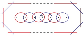
Figure 5.1. The diagram $H_{n}$. Here we have set $n=3$ for simplicity.

Theorem 5.8 gives a new proof of Theorem 1.14 of [HLS] as a direct corollary.

Corollary 5.9.

Given a link $L$ in $S^{3}$, there exists a spectral sequence

$$\widehat{HFL}(\Sigma(L),L)\otimes_{\mathbb{F}_{2}}\mathbb{F}_{2}[\theta,\theta^{-1}]\Rightarrow\widehat{HFL}_{\mathbb{Z}_{2}}(S^{3},L)\otimes_{\mathbb{F}_{2}[\theta]}\mathbb{F}_{2}[\theta,\theta^{-1}],$$

whose pages are isotopy invariants of $L$.

Proof.

Tensoring the spectral sequence of Theorem 5.6 with $\mathbb{F}_{2}[\theta,\theta^{-1}]$ gives a spectral sequence

$$\widehat{HFL}(\Sigma(L),L)\otimes_{\mathbb{F}_{2}}\mathbb{F}_{2}[\theta,\theta^{-1}]\Rightarrow\widehat{HFL}_{\mathbb{Z}_{2}}(\Sigma(L),L)\otimes_{\mathbb{F}_{2}[\theta]}\mathbb{F}_{2}[\theta,\theta^{-1}],$$

and by Theorem 5.8, we have an isomorphism

$$\widehat{HFL}_{\mathbb{Z}_{2}}(\Sigma(L),L)\otimes_{\mathbb{F}_{2}[\theta]}\mathbb{F}_{2}[\theta,\theta^{-1}]\simeq\widehat{HFL}(S^{3},L)\otimes_{\mathbb{F}_{2}}\mathbb{F}_{2}[\theta,\theta^{-1}].$$

∎

6. Application: A transverse invariant refining both the $c_{\mathbb{Z}_{2}}$ and the LOSS invariant

Let $K\subset S^{3}$ be a transverse knot with respect to the standard contact structure $\xi_{std}=\ker(dz-xdy)$. The author constructed in [K] an invariant $c_{\mathbb{Z}_{2}}(\xi_{K})$ as an element of the module $\widehat{HF}_{\mathbb{Z}_{2}}(\Sigma(K))$, which depends only on the transverse isotopy class of $K$. On the other hand, we have the LOSS invariant $\hat{c}(K)$, defined in [LOSSz], which is an element of $\widehat{HFK}(S^{3},K)$, again depending only on the transverse isotopy class of $K$. Therefore it is natural to ask how those two invariants are related.

Recall that we have shown in the previous section that the equivariant knot Floer cohomology $\widehat{HFK}_{\mathbb{Z}_{2}}(\Sigma(K),K)$ is a refinement of both $\widehat{HF}_{\mathbb{Z}_{2}}(\Sigma(K))$ and $\widehat{HFK}(S^{3},K)$. As a topological application of that fact, we will show in this section that there exists a transverse invariant of $K$, as an element of $\widehat{HFK}_{\mathbb{Z}_{2}}(\Sigma(K),K)$, which is a simultaneous refinement of both the equivariant contact class $c_{\mathbb{Z}_{2}}(\xi_{K})$ and the LOSS invariant $\hat{c}(K)$.

We first recall some facts regarding relations between braids and transverse knots. When $(M,\xi)$ is a contact 3-manifold and $h\,:\,M\backslash B\rightarrow S^{1}$ is an open book supporting $\xi$. Then a transverse knot(link) $K\subset M$ is said to be in a braid position with respect to $B$ if $h|_{K}$ is regular, and when $K$ is in a braid position, we call it as a transverse braid. When $(M,\xi)$ is the standard contact $S^{3}$, the theorem of Bennequin[B] tells us that every transverse knot is transversely isotopic to a transverse braid along the $z$-axis. This fact can be directly generalized to the most general case, when $(M,\xi)$ is any contact 3-manifold and $h$ is any open book; in fact, the theorem of Pavelescu[P] tells us that any transverse knot in $M$ is transversely isotopic to a braid position with respect to $h$, and two transverse braids, braided with respect to $B$, are transversely isotopic if and only if they are related by a sequence of braid isotopies, positive Markov moves, and their inverses. This fact leads us to the following definition, made first by Baldwin, Vela-Vick, and Vertesi in [BVV].

Definition 6.1.

Given a contact 3-manifold $(M,\xi)$, an open book $h\,:\,M\backslash B\rightarrow S^{1}$ supporting $\xi$, and a transverse knot $K$ which is in a braid position with respect to $B$, let $S$ be a page of $h$, $F=S\cap K$, and $\phi$ be the monodromy of $h$ which fixes $F$ pointwise. Then the isotopy class of the monodromy $\phi$ rel $F\cup\partial S$ uniquely determines the transverse isotopy class of $K$. So we say that the (transverse isotopy class of) transverse knot $K$ is encoded by the pointed open book $(S,F,\phi)$.

Recall that, given a contact 3-manifold $(M,\xi)$, any two open books of $M$ which support $\xi$ are related by a sequence of isotopies and positive (de)stabilizations. Then, given any pointed open book $(S,F,\phi)$ which encodes a transverse knot $K$ in $(M,\xi)$, we can perform a positive stabilization with respect to any simple arc $a\subset S\backslash F$ satisfying $\partial a\subset\partial S$. Then the pointed open book $(S^{\prime},F^{\prime},\phi^{\prime})$ we obtain by the positive stabilization still encodes the same transverse knot $K$; note that this is a special case of Corollary 2.5 of [BVV].

Using the facts we have stated above, we will give some useful observations on transverse knots in the standard conatct $S^{3}$.

Lemma 6.2.

Let $K\subset(S^{3},\xi_{std})$ be a transverse knot. Then there exists an open book decomposition of $S^{3}$ supporting $\xi_{std}$, such that its binding is disjoint from $K$ and each of its page intersects $K$ transversely at one point.

Proof.

Let $L$ be a Legendrian knot in $(S^{3},\xi_{std})$, whose positive transverse pushoff is $K$. Choose a contact cell decomposition of $(S^{3},\xi_{std})$, so that $L$ is contained in its 1-skeleton $S$. Denote the 1-cells of $S$ which intersects $L$ by $L_{1},\cdots,L_{n}$, and the open book induced by the cell decomposition as $h\,:\,S^{3}\backslash B\rightarrow S^{1}$, where $B$ is the binding. Then a page $\Sigma$ of $h$ is drawn in Figure 6.1. Note that $N(L)\cap\partial(h^{-1}(p))\subset K$, where $N(L)$ is a small neighborhood of $L$; this is because $K$ is a positive pushoff of $L$.

Now perturb $K$ to a knot $K^{\prime}$, so that $h|_{K^{\prime}}$ is monotone but very close to zero in neighborhoods of $L_{1},\cdots,L_{n}$. Then $K^{\prime}$ is clearly in a braid position with respect to $B$. Also, since we can choose our perturbation to be sufficiently $C^{1}$-small, $K^{\prime}$ is also a transverse knot. Therefore $K^{\prime}$ is a 1-strand transverse braid along $B$, so applying a self-contactomorphism of $(S^{3},\xi_{std})$ which takes $K$ to $K^{\prime}$ gives a desired open book. ∎

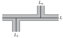
Figure 6.1. The page $\Sigma$ of the open book $h$, near the Legendrian knot $L$.

Lemma 6.3.

Let $K\subset(S^{3},\xi_{std})$ be a transverse knot and $(B_{1},h_{1}),(B_{2},h_{2})$ be open book decompositions of $S^{3}$, supporting $\xi_{std}$, such that $K$ is transversely isotopic to a 1-strand transverse braid along $B_{i}$, for each $i=1,2$. Denote the induced (single-)pointed open books by $(S_{1},p_{1},\phi_{1})$ and $(S_{2},p_{2},\phi_{2})$, respectively. Then $(S_{1},p_{1},\phi_{1})$ and $(S_{2},p_{2},\phi_{2})$ are related by a sequence of isotopies and positive (de)stabilizations.

Proof.

By applying a self-contactomorphism of $(S^{3},\xi_{std})$ to the given open books, we may assume that $K$ intersects the pages of $(B_{1},h_{1})$ and $(B_{2},h_{2})$ transversely at one point. Then, by performing positive stabilizations to $(B_{1},h_{1})$ and $(B_{2},h_{2})$, we may assume that they are induced by a contact cell decomposition of $(S^{3},\xi_{std})$, so that $(B_{1},h_{1})$ is isotopic to $(B_{2},h_{2})$. Also, by performing additional positive stabilizations, we may further assume that, for a Legendrian knot $L$ which has $K$ as its transverse push-off, the given contact cell decomposition contains $L$ in its 1-skeleton. Then, by the argument used in the proof of Lemma 6.2, we deduce that $(S_{1},p_{1},\phi_{1})$ and $(S_{2},p_{2},\phi_{2})$ are isotopic. ∎

To sum up, we have proven the following proposition.

Proposition 6.4.

Any transverse knot in $(S^{3},\xi_{std})$ is encoded by a single-pointed open book, and any two single-pointed open books encoding the same transverse knot in $(S^{3},\xi_{std})$ are related by a sequence of isotopies and positive (de)stabilizations.

Proof.

This is a direct consequence of Lemma 6.2 and Lemma 6.3. ∎

Now we will see how to translate a single-pointed open book, which encodes a transverse knot $K$ in $(S^{3},\xi_{std})$, to an element in $\widehat{HFK}_{\mathbb{Z}_{2}}(\Sigma(K),K)$. Given such a single-pointed open book $(S,p,\phi)$, choose an arc-basis $\mathbf{a}=\{a_{1},\cdots,a_{n}\}$ of $S$, where the arcs in $\mathbf{a}$ do not contain $p$. Then consider the following objects.

• $\Sigma=(S\times\{0,1\})/\sim$ where $(x,0)\sim(x,1)$ for any $x\in\partial S$

• For each $i=1,\cdots,n$, $b_{i}$ is the arc in $S$ given by perturbing $a_{i}$ slightly, so that $a_{i}$ intersects $b_{i}$ transversely at one point $x_{i}$, where the intersection is positive.

• $\boldsymbol{\alpha}=\{(a_{i}\times\{0\})\cup(a_{i}\times\{1\})|i=1,\cdots,n\}$

• $\boldsymbol{\beta}=\{(b_{i}\times\{0\})\cup(\phi(b_{i})\times\{1\})|i=1,\cdots,n\}$

• $z=(p,0)$, $w=(p,1)$ in $\Sigma$

Then the 5-tuple $H_{(S,p,\phi,\mathbf{a})}=(\Sigma,\boldsymbol{\alpha},\boldsymbol{\beta},z,w)$ is a knot Heegaard diagram representing $K$ in $S^{3}$, and its branched double cover $\hat{H}$ along $\{z,w\}$ is a $\mathbb{Z}_{2}$-invariant knot Heegaard diagram representing $K$ in $\Sigma(K)$, so that we have

$$\widehat{HFK}_{\mathbb{Z}_{2}}(\Sigma(K),K)\simeq\widehat{HF}_{\mathbb{Z}_{2}}(\hat{H})\simeq H^{\ast}(\text{RHom}_{\mathbb{F}_{2}[\mathbb{Z}_{2}]}(\widehat{CF}(\hat{H}),\mathbb{F}_{2}))$$

by Lemma 5.2. So, if we denote the inverse image of $\{x_{1},\cdots,x_{n}\}$ under the branched covering map by $\mathbf{x}_{(S,p,\phi,\mathbf{a})}$, then since $\mathbf{x}_{(S,p,\phi,\mathbf{a})}$ is a $\mathbb{Z}_{2}$-invariant cocycle in $\widehat{CF}(\hat{H})$, the element $\mathbf{x}_{(S,p,\phi,\mathbf{a})}\otimes 1$ in $\text{RHom}_{\mathbb{F}_{2}[\mathbb{Z}_{2}]}(\widehat{CF}(\hat{H}),\mathbb{F}_{2})$ is a cocycle, which then corresponds to a cocycle in $\widehat{CFK}_{\mathbb{Z}_{2}}(\Sigma(K),K)$. We will denote its cohomology class as $\hat{\mathcal{T}}_{\mathbb{Z}_{2}}(S,p,\phi,\mathbf{a})$. Also, we will denote $\widehat{HF}_{\mathbb{Z}_{2}}(\hat{H})$ as $\widehat{HFK}_{\mathbb{Z}_{2}}(S,p,\phi,\mathbf{a})$, and call the tuple $(S,p,\phi,\mathbf{a})$ as a single-pointed arc diagram.

Lemma 6.5.

Let $S$ be a compact oriented surface with boundary, $p$ be a point in the interior of $S$, and $\mathbf{a}_{1},\mathbf{a}_{2}$ be arc bases of $S$ whose arcs do not contain $p$. Then $\mathbf{a}_{1}$ and $\mathbf{a}_{2}$ are related by a sequence of isotopies and arc-slides, where the isotopies are performed outside $p$.

Proof.

We only have to prove that we can replace an isotopy through $p$ by a sequence of isotopies and handleslides performed in $S\backslash\{p\}$. To prove this, choose an arc $a\in\mathbf{a}_{1}$ and suppose that we want to isotope $a$ to another simple arc $a^{\prime}$, where $p\notin a^{\prime}$, $a\cap a^{\prime}=\emptyset$, and $a,a^{\prime}$ cobound a strip $R\subset S$ where $p\in R$. Cutting $S$ along the arcs in $\mathbf{a}_{1}\backslash\{a\}$ gives an annulus $A$, where the two endpoints of $a$ lie in different components of $\partial A$ . Here, $A\backslash(a\cup a^{\prime})$ is a disjoint union of a disk $D$ with the strip $R$. Then, by a sequence of isotopies and arc-slides in $D$, we can replace $a$ by $a^{\prime}$, as in Figure 6.2. Since $p\notin D$, we see that the isotopies we have used are performed outside $p$. ∎

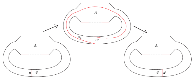
Figure 6.2. The arc $a_{1}$ is obtained from $a$ by a sequence of arc-slides, and $a^{\prime}$ is obtained from $a_{1}$ again by a sequence of arc-slides. During the process, the arc-slides we perform do not pass through the basepoint $p$.

Definition 6.6.

When two single-pointed arc diagrams $(S,p,\phi,\mathbf{a})$ and $(S^{\prime},p^{\prime},\phi^{\prime},\mathbf{a}^{\prime})$ are related by either an isotopy outside $p$, an arc-slide, or a stabilization, we say that they are related by a basic move. Note that a basic move induces a map

$$\widehat{HFK}_{\mathbb{Z}_{2}}(S^{\prime},p^{\prime},\phi^{\prime},\mathbf{a}^{\prime})\rightarrow\widehat{HFK}_{\mathbb{Z}_{2}}(S,p,\phi,\mathbf{a}).$$

Lemma 6.7.

Suppose that two single-pointed arc diagrams $(S,p,\phi,\mathbf{a})$ and $(S^{\prime},p^{\prime},\phi^{\prime},\mathbf{a}^{\prime})$ are related by a basic move. Then the induced map

$$\widehat{HFK}_{\mathbb{Z}_{2}}(S^{\prime},p^{\prime},\phi^{\prime},\mathbf{a}^{\prime})\rightarrow\widehat{HFK}_{\mathbb{Z}_{2}}(S,p,\phi,\mathbf{a})$$

takes $\hat{\mathcal{T}}_{\mathbb{Z}_{2}}(S^{\prime},p^{\prime},\phi^{\prime},\mathbf{a}^{\prime})$ to $\hat{\mathcal{T}}_{\mathbb{Z}_{2}}(S,p,\phi,\mathbf{a})$.

Proof.

The branched double covers of $(S,p,\phi,\mathbf{a})$ and $(S^{\prime},p^{\prime},\phi^{\prime},\mathbf{a}^{\prime})$, along $p$ and $p^{\prime}$, respectively, are related by two basic moves, performed in a $\mathbb{Z}_{2}$-invariant way. Thus the conclusion follows from the argument used to prove the invariance of the contact classes of contact 3-manifolds; see Section 3 of [HKM] for details. ∎

From the things we have proven so far, we see that we have found a well-defined transverse invariant. Although we have not proven the naturality of $\widehat{HFK}_{\mathbb{Z}_{2}}(\Sigma(K),K)$, we can still define its well-defined element, which depends only on the transverse isotopy class of $K$ in $S^{3}$.

Theorem 6.8.

The element $\hat{\mathcal{T}}_{\mathbb{Z}_{2}}(S,p,\phi,\mathbf{a})$ depends only on the transverse isotopy class of transverse knots which $(S,p,\phi,\mathbf{a})$ encodes.

Proof.

This follows directly from Lemma 6.5 and Lemma 6.7. ∎

Definition 6.9.

Given a (transverse isotopy class of) transverse knot $K$ in $(S^{3},\xi_{std})$, we define $\hat{\mathcal{T}}_{\mathbb{Z}_{2}}(S,p,\phi,\mathbf{a})$, for any single-pointed arc diagram $(S,p,\phi,\mathbf{a})$ encoding $K$, as $\hat{\mathcal{T}}_{\mathbb{Z}_{2}}(K)$.

Finally, we will see that $\hat{\mathcal{T}}_{\mathbb{Z}_{2}}(K)$ is a transverse invariant which is a refinement of both the hat-flavored LOSS invariant $\hat{\mathcal{T}}(K)\in\widehat{HFK}(S^{3},K)$, and the $\mathbb{Z}_{2}$-equivariant contact class $c_{\mathbb{Z}_{2}}(\xi_{K})\in\widehat{HF}_{\mathbb{Z}_{2}}(\Sigma(K))$, defined in [K].

Theorem 6.10.

For any transverse knot $K$ in $(S^{3},\xi_{std})$, there exists a localization isomorphism

$$\widehat{HFK}_{\mathbb{Z}_{2}}(\Sigma(K),K)\otimes_{\mathbb{F}_{2}[\theta]}\mathbb{F}_{2}[\theta,\theta^{-1}]\xrightarrow{\sim}\widehat{HFK}(S^{3},K)\otimes_{\mathbb{F}_{2}}\mathbb{F}_{2}[\theta,\theta^{-1}],$$

as defined in Theorem 5.8, which maps $\hat{\mathcal{T}}_{\mathbb{Z}_{2}}(K)\otimes 1$ to $\hat{\mathcal{T}}(K)\otimes 1$.

Proof.

Let $(S,p,\phi,\mathbf{a})$ be a single-pointed arc diagram encoding $K$, so that $K$ is in a braid position with respect to the binding $B=\partial S$. For a positive integer $n$, consider the transverse braid $K_{n}$ given by applying postive Markov moves $n$ times to $K$, and denote the $(n+1)$-pointed arc diagram encoding the braid $K_{n}$ by $(S,\mathbf{p}_{n},\phi,\mathbf{a}_{n})$. Here, $\mathbf{p}_{n}=\{p,p_{1},\cdots,p_{n}\}$ where $p_{1},\cdots,p_{n}$ are pointes added by Markov moves, and $\mathbf{a}_{n}$ is the arc basis given by adding to $\mathbf{a}$ small arcs connecting the points $p_{i}$ to the component of $\partial S$ where the $i$th Markov move was taken. Then, under the isomorphism

$$\widehat{HFK}_{\mathbb{Z}_{2}}(S,p,\phi,\mathbf{a})\otimes_{\mathbb{F}_{2}}V_{n}\xrightarrow{\sim}\widehat{HFK}_{\mathbb{Z}_{2}}(S,\mathbf{p}_{n},\phi,\mathbf{a}_{n}),$$

the element $\hat{\mathcal{T}}_{\mathbb{Z}_{2}}(K)\otimes c$, where $c$ denotes the top class in $V_{n}=(\mathbb{F}_{2}^{2})^{\otimes n}$, is mapped to the cohomology class of the cocycle $\mathbf{x}_{H_{(S,\mathbf{p}_{n},\phi,\mathbf{a}_{n})}}$.

Now, when $n$ is sufficiently big, $(S,\mathbf{p}_{n},\phi,\mathbf{a}_{n})$ is related by a sequence of isotopies, arc-slides, and positive (de)stabilizations to a pointed diagram of genus zero. So, by the argument used in the proof of Theorem 5.8, together with Lemma 6.7 applied to multi-pointed open books, we have a localization isomorphism

$$\widehat{HFK}_{\mathbb{Z}_{2}}(S,\mathbf{p}_{n},\phi,\mathbf{a}_{n})\otimes_{\mathbb{F}_{2}[\theta]}\mathbb{F}_{2}[\theta,\theta^{-1}]\xrightarrow{\sim}\widehat{HFK}(S,\mathbf{p}_{n},\phi,\mathbf{a}_{n})\otimes_{\mathbb{F}_{2}}\mathbb{F}_{2}[\theta,\theta^{-1}],$$

which maps $\mathbf{x}_{H_{(S,\mathbf{p}_{n},\phi,\mathbf{a}_{n})}}\otimes 1$ to $\hat{t}(K_{n})\otimes 1$, where $\hat{t}(K_{n})$ is the image of the BRAID invariant of the transverse braid $K_{n}$, defined in [BVV], under the natural map from $HFK^{-}$ to $\widehat{HFK}$. Also, by the LOSS=BRAID theorem (Theorem 5.1 of [BVV]) and the construction of localization map in [SS], the isomorphism

$$\widehat{HFK}(S^{3},K)\otimes V_{n}\xrightarrow{\sim}\widehat{HFK}(S,\mathbf{p}_{n},\phi,\mathbf{a}_{n})$$

maps $\hat{\mathcal{T}}(K)\otimes c$ to $\hat{t}(K_{n})$. Therefore there exists an isomorphism

$$\widehat{HFK}_{\mathbb{Z}_{2}}(\Sigma(K),K)\otimes_{\mathbb{F}_{2}[\theta]}\mathbb{F}_{2}[\theta,\theta^{-1}]\xrightarrow{\sim}\widehat{HFK}(S^{3},K)\otimes_{\mathbb{F}_{2}}\mathbb{F}_{2}[\theta,\theta^{-1}]$$

which maps $\hat{\mathcal{T}}_{\mathbb{Z}_{2}}(K)\otimes 1$ to $\hat{\mathcal{T}}(K)\otimes 1$ . ∎

Proving that $\hat{\mathcal{T}}_{\mathbb{Z}_{2}}(K)$ is a refinement of $c_{\mathbb{Z}_{2}}(K)$ is a bit more difficult, as it needs an extension of the definition of $c_{\mathbb{Z}_{2}}(\xi_{K})$. Recall that, for a transverse knot $K$ in $(S^{3},\xi_{std})$, the $\mathbb{Z}_{2}$-equivariant contact class $c_{\mathbb{Z}_{2}}(\xi_{K})$ is defined as follows.

• Choose a multi-pointed genus zero open book $(D,\mathbf{p}=\{p_{1},\cdots,p_{n}\},\phi)$ which encodes $K$.

• Choose a system of pairwise disjoint arcs $\mathbf{a}=\{a_{1},\cdots,a_{n}\}$ such that, for each $i=2,\cdots,n$, $a_{i}$ starts from $p_{i}$ and ends at a point in $\partial D$.

• Taking the branched double cover of $(D,\phi,\mathbf{a}\backslash\{a_{1}\})$, branched along $\mathbf{p}$, gives a $\mathbb{Z}_{2}$-invariant arc diagram $(\Sigma,\phi,\tilde{\mathbf{a}})$, where the point $p_{1}$ now works as a basepoint.

• Applying Honda-Kazez-Matic construction of contact classes, as given in the paper [HKM], gives an element $EH_{\mathbb{Z}_{2}}(\xi_{K})\in\widehat{CF}_{\mathbb{Z}_{2}}(\Sigma,\phi,\tilde{\mathbf{a}})$, which turns out to be a cocycle which depends only on the transverse isotopy class of $K$; see [K] for details.

• The cohomology class of $EH_{\mathbb{Z}_{2}}(\xi_{K})$ is denoted as $c_{\mathbb{Z}_{2}}(\xi_{K})$.

We will now extend this definition to multi-pointed open books of arbitrary genera.

Definition 6.11.

Let $S$ be a compact oriented surface with boundary and $\mathbf{p}\subset\text{int}(S)$ be a finite subset, say $\mathbf{p}=\{p_{1},\cdots,p_{n}\}$. Then an extended arc basis of the multi-pointed surface $(S,\mathbf{p})$ is a set $\mathbf{a}=\{a_{1}^{w},\cdots,a_{m}^{w},a_{1}^{h},\cdots,a_{n}^{h}\}$ of pairwise disjoint simple arcs, which satisfies the following conditions. Here, the arcs $a_{i}^{w}$ are called whole arcs, and $a_{j}^{h}$ are called half arcs.

• $\{a_{1}^{w},\cdots,a_{m}^{w}\}$ is an arc basis of $S$.

• For each $i=1,\cdots,n$, the arc $a_{i}^{h}$ starts from $p_{i}$ and ends at a point in $\partial S$.

Given a multi-pointed open book $(S,\mathbf{p},\phi)$ encoding a transverse knot $K$ in $(S^{3},\xi_{std})$, choose an extended arc basis $\mathbf{a}$ of $(S,\mathbf{p})$ together with a distinguished element $p_{1}\in\mathbf{p}$. Then, as in the genus zero case, taking the branched double cover of $(S,\phi,\mathbf{a}\backslash\{a_{1}^{h}\})$ along $\mathbf{p}$, where $a_{1}^{h}$ is the half arc in $\mathbf{a}$ which contains $p_{1}$, gives a $\mathbb{Z}_{2}$-invariant arc diagram $(\Sigma,\phi,\tilde{\mathbf{a}})$, where $p_{1}$ is now a basepoint in $\Sigma\backslash\cup\tilde{\mathbf{a}}$. Applying Honda-Kazez-Matic construction then gives a canonical element $EH_{\mathbb{Z}_{2}}(S,\mathbf{p},\phi,\mathbf{a},p_{1})$.

Definition 6.12.

The argument used to prove that $EH_{\mathbb{Z}_{2}}(\xi_{K})$ is a cocycle can be directly applied to show that $EH_{\mathbb{Z}_{2}}(S,\mathbf{p},\phi,\mathbf{a},p_{1})$ is also a cocycle in $\widehat{CF}_{\mathbb{Z}_{2}}(\Sigma,\phi,\tilde{\mathbf{a}},p_{1})$. So we denote its cohomology class as $c_{\mathbb{Z}_{2}}(S,\mathbf{p},\phi,\mathbf{a},p_{1})$.

When $(S,\mathbf{p},\phi)$ is a multi-pointed open book, $p_{1}\in\mathbf{p}$ is a distinguished point, and $\mathbf{a}$ is an extended arc basis of $(S,\mathbf{p})$, then we call the tuple $(S,\mathbf{p},\phi,\mathbf{a})$ as an extended arc diagram. The difference between using genus zero extended arc diagrams and using diagrams of arbitrary genera is that we now have four possible types of arc-slides. As usual, we call isotopies and arc-slides as basic moves. Note that the HKM construction applied to an extended arc diagram gives an extended bridge diagram, and arc-slides of type I/II/III/IV correspond to the same types of handleslides.

Isotopy

We can perform an isotopy to arcs in an extended arc basis $\mathbf{a}$ of a multi-pointed surface $(S,\mathbf{p})$. Here, the isotopies must not pass through points in $\mathbf{p}$.

Arc-slide of type I

We can perform an (ordinary) arc-slide of an whole arc along another whole arc in an extended arc basis $\mathbf{a}$, outside the basepoint $p_{1}$ and the half-arcs in $\mathbf{a}$.

Arc-slide of type II

Given a whole arc $a^{w}$ and a half arc $a^{h}$ in an extended arc basis $\mathbf{a}$, we can replace $a^{w}$ by another whole arc $a_{1}^{w}$ if $a_{1}^{w}$ does not intersect the arcs in $\mathbf{a}\backslash\{a^{w}\}$, $a_{1}^{w}$ intersects $a^{w}$ transversely at one point, and $S\backslash(a^{w}\cup a_{1}^{w})$ contains a triangle component $T$ such that $a^{h}\subset T$.

Arc-slide of type III

Given a half arc $a^{h}$ and a whole arc $a^{w}$ in an extended arc basis $\mathbf{a}$, we can replace $a^{h}$ by another arc $a_{1}^{h}$ if $a^{h}\cap a_{1}^{h}$ is a point in $\mathbf{p}$, the interior of $a_{1}^{h}$ does not intersect the arcs in $\mathbf{a}$, and the arcs $a^{h},a^{w},a_{1}^{h}$ bound a strip in $S$.

Arc-slide of type IV

Given two half arcs $a_{1}^{h},a_{2}^{h}$ in an extended arc basis $\mathbf{a}$, we can replace $a_{1}^{h}$ by another arc $a_{1^{\prime}}^{h}$ if $a_{1}^{h}\cap a_{1^{\prime}}^{h}$ is a point in $\mathbf{p}$, the interior of $a_{1^{\prime}}^{h}$ does not intersect the arcs in $\mathbf{a}$, and $S\backslash(a_{1}^{h}\cup a_{1^{\prime}}^{h})$ contains a triangle component $T$ satisfying $a_{2}^{h}\subset T$.

Lemma 6.13.

Any two arc bases of a multi-pointed surface $(S,\mathbf{p})$ are related by a sequence of isotopies and arc-slides.

Proof.

This can be seen easily by combining the argument used in the proof of Lemma 6.5 together with the proof of Proposition 5.3 in [K]. ∎

Proposition 6.14.

Let $(S,\mathbf{p},\phi,\mathbf{a},p_{1})$ be an extended arc diagram, where $(S,\mathbf{p},\phi)$ encodes a transverse knot $K$ in $(S^{3},\xi_{std})$. Then $c_{\mathbb{Z}_{2}}(S,\mathbf{p},\phi,\mathbf{a},p_{1})$ depends only on the transverse isotopy class of $K$.

Proof.

The proof is essentially the same as in the proof of invariance of $c_{\mathbb{Z}_{2}}(\xi_{K})$ for genus zero open books. See Section 5 of [K] for details. ∎

Finally, we can prove that for transverse knots $K$ in $(S^{3},\xi_{std})$, $\hat{\mathcal{T}}_{\mathbb{Z}_{2}}(K)$ is a refinement of $c_{\mathbb{Z}_{2}}(\xi_{K})$.

Theorem 6.15.

For any transverse knot $K$ in $(S^{3},\xi_{std})$, the natural map

$$\widehat{HFK}_{\mathbb{Z}_{2}}(\Sigma(K),K)\rightarrow\widehat{HF}_{\mathbb{Z}_{2}}(\Sigma(K))$$

maps $\hat{\mathcal{T}}_{\mathbb{Z}_{2}}(K)$ to $c_{\mathbb{Z}_{2}}(\xi_{K})$.

Proof.

Let $(S,p,\phi,\mathbf{a})$ be a single–pointed arc diagram, where $(S,p,\phi)$ encodes $K$. Choose a simple arc $a^{h}$ on $S\backslash\cup\mathbf{a}$ which starts from $p$ and ends at a point in $\partial S$. Then the image of $\mathbf{x}_{H_{(S,p,\phi,\mathbf{a})}}$ in the chain level is given by $EH_{\mathbb{Z}_{2}}(S,p,\phi,\mathbf{a}\cup\{a^{h}\},p)$. Since $\hat{\mathcal{T}}_{\mathbb{Z}_{2}}(K)$ is the cohomology class of $\mathbf{x}_{H_{(S,p,\phi,\mathbf{a})}}$, and the cohomology class of $EH_{\mathbb{Z}_{2}}(S,p,\phi,\mathbf{a}\cup\{a^{h}\},p)$ is equal to $c_{\mathbb{Z}_{2}}(\xi_{K})$ by 6.14, we see that $\hat{\mathcal{T}}_{\mathbb{Z}_{2}}(K)$ is mapped to $c_{\mathbb{Z}_{2}}(\xi_{K})$. ∎

References

[B]D. Bennequin, Entrelacements et equations de
Pfaff, Asterisque 107-108 (1983), 87-161. English version: Russian
Math.Surveys, 44, No. 3 (1989), 1-65
[BVV]J. A. Baldwin, D. S. Vela-Vick, and
V. Vertesi, On the equivalence of Legendrian and transverse invariants
in knot Floer homology, Geom. Topol.17 (2013), no. 2, 925–974
[HLS]K. Hendricks, R. Lipschitz, and S. Sarkar,
A flexible construction of equivariant Floer homology and applications,
arXiv preprint arXiv:1510.02449 (2015)
[HKM]K. Honda, W. H. Kazez, and G. Matic, On the contact
class in Heegaard Floer homology, arXiv preprint math/0609734 (2006)
[JT]A. Juhasz and D. Thurston, Naturality
and mapping class groups in Heegaard Floer homology, arXiv preprint
math.GT/1210.4996.
[K]S. Kang, A transverse knot invariant from Z2-equivariant
Heegaard Floer cohomology, arXiv preprint arXiv:1802.00351 (2018).
[L]R. Lipschitz, A cylindrical reformulation
of Heegaard Floer homology, Geometry & Topology 10.2 (2006), 955-1096
[LOSSz]P. Lisca, P. Ozsvath, A. I. Stipsicz, and
Z. Szabo, Heegaard Floer invariants of Legendrian knots in contact
three-manifolds, Journal of European Mathematical Society 11 (2009),
no. 6, 1307– 1363
[OSz]P. Ozsvath and Z. Szabo, Holomorphic disks
and topological invariants for closed threemanifolds, Ann. of Math.
.2/ 159 (2004) 1027–115
[P]E. Pavelescu, Braiding knots in contact 3-manifolds,
Pacific J. Math. 253 (2011) 475– 487
[SS] P. Seidel and I. Smith, Localization
for involutions in Floer cohomology, Geometric and Functional Analysis
20.6 (2010), 1464-1501
[SW]S. Sarkar and J. Wang, An algorithm for
computing some Heegaard Floer homologies, Annals of mathematics (2010),
1213-1236.