Net-baryon multiplicity distribution consistent with lattice QCD
Abstract
We determine the net-baryon multiplicity distribution which reproduces all cumulants measured so far by lattice QCD. We present the dependence on the volume and temperature of this distribution. We find that for temperatures and volumes encountered in heavy ion reactions, the multiplicity distribution is very close to the Skellam distribution, making the experimental determination of it rather challenging. We further provide estimates for the statistics required to measure cumulants of the net-baryon and net-proton distributions.
I Introduction
In recent years is has been realized that the fluctuations of conserved charges provide experimental access to the phase structure of QCD Jeon and Koch (2000); Asakawa et al. (2000); Stephanov (2009); Skokov et al. (2011); Stephanov (2011); Luo et al. (2012); Luo and Xu (2017); Herold et al. (2016); Zhou et al. (2012); Wang and Yang (2012); Karsch and Redlich (2011); Schaefer and Wagner (2012); Chen et al. (2011); Fu et al. (2010); Cheng et al. (2009). In particular the cumulants of the net-baryon number distribution have been found to be sensitive to the details of the transition from hadron gas to the quark-gluon plasma. Not only are they sensitive probes for a possible critical point Stephanov (2009) but they may also reveal the chiral critical behavior underlying the cross-over transition Aoki et al. (2006); Borsanyi et al. (2010); Bazavov et al. (2012) at vanishing net-baryon chemical potential Skokov et al. (2011); Karsch and Redlich (2011). This insight has motivated the experimental measurement of these cumulants Adamczyk et al. (2014); Rustamov (2017). Since the detection of neutrons is difficult if not impossible in these experiments, the present measurements are restricted to net-proton cumulants, which however, can be related to the baryon cumulants Kitazawa and Asakawa (2012a, b). Also, the experimental data need to be corrected for global baryon number conservation Bzdak et al. (2013) and detector specific effects such as efficiencies etc. Bzdak and Koch (2012); Luo (2015a); Bzdak et al. (2016); Braun-Munzinger et al. (2016, 2017); Kitazawa (2016); He and Luo (2018); Nonaka et al. (2018).
The cumulants of the net-baryon number distribution for a system at vanishing net-baryon chemical potential can be calculated from lattice QCD and at present results are available up the eighth order, Bazavov et al. (2017); Borsanyi et al. (2018). However, so far it has not been possible to extract the full net-baryon multiplicity distribution directly from lattice QCD. The knowledge of this multiplicity distribution would be not only of scientific interest but also has some practical importance. For example, one can calculate to which extent the multiplicity distribution consistent with lattice QCD deviates from that of uncorrelated particles, the Skellam distribution. In addition, one can determine how far one has to sum over the multiplicity distribution in order to get a reasonable approximation for a given cumulant. Furthermore, as we shall discuss in some detail in the Appendix, one can apply the delta method Davison (2003); Luo (2015a); Luo and Xu (2017) in order to estimate the needed statistics for the measurement of net-baryon cumulants.
The net-baryon number multiplicity distribution has been determined based on an effective model of QCD Morita et al. (2013) as well as from the hadron resonance gas model Braun-Munzinger et al. (2011). In this paper we will construct the net-baryon multiplicity distribution based on lattice QCD results Vovchenko et al. (2017) and on the cluster expansion model (CEM) described in Vovchenko et al. (2018a). As demonstrated in Vovchenko et al. (2018a, b) the CEM reproduces all net-baryon number cumulants determined by lattice QCD so far. Consequently the cumulants of the constructed multiplicity distribution agree with all cumulants presently known from lattice QCD (up to eighth order). Thus, we consider the extracted multiplicity distribution as the best presently available template. We note that an alternative virial expansion has been proposed in Almasi et al. (2018), which also fits the presently available lattice data within errors. While both expansions have quite different asymptotic behavior of the virial coefficients, the resulting multiplicity distributions are very similar as we shall discuss.
This paper is organized as follows. In the next section be briefly review the CEM and show how it can be used to extract the net-baryon multiplicity distribution. Next, we present the results and finish with a discussion, which includes an estimate of the required statistics for the measurement of net-baryon and net-proton cumulants.
II Net-baryon multiplicity distribution
To illustrate how one can extract the multiplicity distribution, let us start with the fugacity expansion of the pressure
| (1) |
where is the ratio of baryon chemical potential over temperature and are coefficients to be determined. Therefore, the partition function, , can be written as
| (2) |
On the other hand the partition function can also be written as a sum involving all the net-baryon partition functions, ,
| (3) |
Here and in the following we denote the net-baryon number by . In the previous equation we made use of charge symmetry to relate . In the present paper we are interested in the case of vanishing baryon chemical potential, where the cumulants are measured on the lattice up to the eighth order. Given the , the probability to have net-baryons at vanishing chemical potential, , is then given by
| (4) |
Therefore, the task at hand is to determine the net-baryon partition function, . To this end we equate the two expressions for the partition function, Eqs. (2) and (3), and divide both sides by the partition function taken at ,
| (5) | |||||
We note that the normalization with removes the dependence of the left hand side on the virial coefficient and thus the sums start at . Upon rotating to imaginary chemical potential (see also Morita et al. (2013)), , the above equation turns into
| (6) |
so that the -net-baryon probabilities, , result from simple Fourier transform
| (7) |
Therefore, given the coefficients , one can determine the multiplicity distribution . Furthermore, since the cumulants are given by
| (8) |
they can be readily calculated either using Eq. (1) or directly from the multiplicity distribution, . This provides an important cross check for the numerical Fourier transform required.
In order to proceed, all we need then are the coefficients, . Here, we make use of the recent work by Vovchenko et al. Vovchenko et al. (2018a). In this paper the authors used a cluster model to determine the coefficients provided the first two coefficients, and are known. In Vovchenko et al. (2017) the first four coefficients, have been determined by lattice QCD methods. Taking the lattice results for and as input, the cluster model of Vovchenko et al. (2018a) not only reproduces and obtained from lattice QCD, but also is able to reproduce the baryon number cumulants obtained from lattice QCD up to eighth order, which is the highest presently available (for the quality of the agreement see Vovchenko et al. (2018a, b)). Given the success of this cluster model, we consider it to be a suitable model to determine a more or less realistic net-baryon multiplicity distribution. Also, alternative virial expansion of Ref. Almasi et al. (2018) leads to nearly identical results. We further note, that model dependence may be systematically reduced by extracting ever higher coefficients from lattice QCD. Finally, we recall from Refs. Vovchenko et al. (2018a, b), that in their cluster expansion model the above sums can be carried out analytically, which is helpful for carrying out the Fourier transform.
| (9) |
where
| (10) |
and is the polylogarithm.111An analogous sum with can by obtained by .
III Results
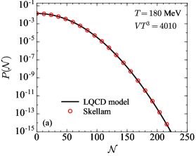
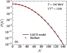
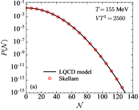
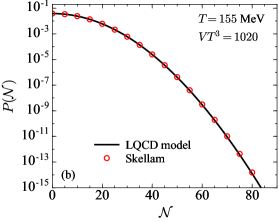
After having introduced the method for extracting the multiplicity distribution let us now turn to the results. Given the cluster model of Vovchenko et al. (2018a) the kernel of the Fourier integral of Eq. (7) is straightforward to determine (see Eqs. (9) and (10)). We further note that the kernel of the Fourier integral depends on the volume so that with increasing volume it becomes an ever steeper function localized around . As a result, with increasing ever higher Fourier components become relevant. This of course simply reflects the fact that for fixed temperature the average number of baryons and anti-baryons increases with the volume resulting in an ever broader distribution of the net-baryon number. In the following, we will consider two volumes, which corresponds to the chemical freeze out volume extracted Andronic et al. (2018) from data taken by the ALICE collaboration at the LHC and which is the estimated chemical freeze out volume for the top RHIC energy () Andronic (2014). For the multiplicity distributions shown in the following we have ensured that the maximum value for , , is such that all cumulants up to order agree within one percent if calculated either from Eq. (8) or in terms of moments of the multiplicity distribution, . We will consider two values for the temperature. The lower one, , corresponds the chemical freeze-out temperature extracted from hadron-yield systematics Andronic et al. (2018). We also consider , where the cumulants are substantially different. For example at while at Bazavov et al. (2017). This will give us an idea to which extent the multiplicity distribution depends on the value of the cumulants. The values for the input parameters are , for and , for .
In Fig. 2 we show the multiplicity distribution, , for a system at temperature . Panel (a) corresponds to the volume extracted for LHC and panel (b) for that at the top RHIC energy, corresponding to and , respectively. Note that we show the distributions only for positive since it is symmetric with respect to . In addition, as red circles we show the corresponding Skellam distribution
| (11) |
where is the modified Bessel function of the first kind. We adjust the parameter such that the Skellam distribution and the model distribution have the same variance,
| (12) |
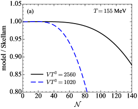
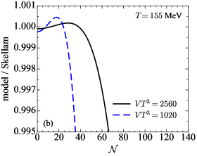
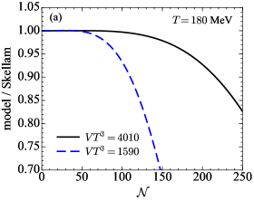
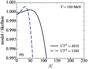
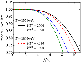
that is since for Skellam (of course ). Here is the second order cumulant, consistent with lattice QCD. The difference between the model distribution, , which is consistent with the cumulants from lattice QCD, and the Skellam distribution, where all cumulants are the same, , is barely visible. To show the difference more clearly, in Fig. 2 we show the ratio of . In panel (a) we plot the ratio over the same range as in the previous figure, and we see for the smaller volume this ratio drops faster. In panel (b) we zoom into the region where the ratio is approximately unity. We see that in both cases the ratio exceeds one, however, only by less than 0.1%. Also, the maximum in case of the RHIC volume is more pronounced. To see how things change with temperature, we show the resulting multiplicity distributions also for a temperature of in Figs. 4 and 4. We used the same volumes used in Figs. 2 and 2 so that the factor and thus the width of the distribution increase with the temperature. Although the cumulants are quite different at , comparing Figs. 2 and 4 we find that the deviation from the Skellam distribution does not change significantly. For both temperatures we have observed a volume dependence of the multiplicity distributions, which qualitatively is not surprising, as the width increases with the volume . To remove this rather trivial effect, in Fig. 5 we plot the ratios as a function of , where is respective width for each volume and temperature. Obviously the distribution does not simply scale with the width.
| , (Fig. 1(a)) | 86 () | 118 () | 137 () |
| , (Fig. 1(b)) | 52 () | 72 () | 83 () |
| , (Fig. 3(a)) | 161 () | 211 () | 249 () |
| , (Fig. 3(b)) | 98 () | 128 () | 150 () |
IV Discussion and Conclusion
After having presented the multiplicity distributions which are consistent with the cumulants determined from lattice QCD a few points are worth discussing
-
(i)
Our main finding is that the deviation of the LQCD-based net-baryon multiplicity distribution from the Skellam distribution with the same width (or same second order cumulant) is very small for all cases considered. For the more realistic temperature of and a value of the probability as small as the difference is less than 15% for LHC energies and at best 20% in case of top RHIC energies (see Figs. 2 and 2). The same qualitative result is found when using the virial expansion of Ref. Almasi et al. (2018), which also reproduces the lattice cumulants within errors but has different asymptotic behavior of the virial coefficients, . In this case, as shown in Fig. 6, the ratio to the corresponding Skellam distribution is somewhat closer to unity as compared to the model of Vovchenko et al. (2018a) (see Fig. 2(a)), while the multiplicity distributions look virtually identical to those shown in Fig. 2. Specifically, the deviations are for LHC and for RHIC at the points where . Therefore, given the small deviation from a Skellam distribution and the fact that the direct measurement of a multiplicity distribution involves unfolding of efficiency corrections (see, e.g., Bzdak et al. (2016)) it is very unlikely that a meaningful extraction of the multiplicity distribution is possible in practice.
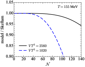
Figure 6: The ratios (model over Skellam) for the virial expansion model of Ref. Almasi et al. (2018). -
(ii)
Here we have discussed the multiplicity distribution of net-baryons. In experiment one is usually restricted to the measurement of net-protons. As discussed in Kitazawa and Asakawa (2012a), assuming fast isospin exchange the net-proton distribution can be derived from the net-baryon distribution by folding with a binomial distribution with Bernoulli probability of . This, however, brings the distribution even closer to a Skellam distribution Bzdak and Koch (2012).
-
(iii)
In order to provide some guidance how sensitive the cumulants are to the tails of the distribution, in Table 1 we provide the minimum range one has to sum the multiplicity distribution over in order to get a certain cumulant ratio within 5% of the correct value ( is reduced by 3 if for 10% accuracy). We also list the probability at this point. For example, in order to obtain within 5% for the LHC at the realistic freeze-out temperature of (), we need to sum until , where the probability is as low as .
-
(iv)
To estimate the required statistics for the measurement of a given cumulant, one either samples the multiplicity distribution or equivalently makes use the delta method Davison (2003); Luo (2015a); Luo and Xu (2017). This is discussed in some detail in the Appendix. Using the delta method, one finds that the relative error for the measurement of a cumulant of given order , , in principle depends on all cumulants up to order . However, as shown in the Appendix, in case of QCD where the cumulant ratios are of order one, the leading term involving only the second order cumulant dominates the absolute error, . The relative error, of course depends on the actual magnitude of . As shown in detail in the Appendix, to leading order the relative error the fourth and sixth order cumulants are given by:
(13) (14) where denotes the cumulant ratio of the n-th order cumulant over the second order cumulant. Given the relative error, one can estimate the number of events required to measure the cumulants and, as discussed in the Appendix, we find that for the LHC conditions at least and events are needed to measure and at 10% accuracy, respectively. For RHIC one needs at least and . As further discussed in the Appendix, the situation is somewhat less statistics hungry in case of net protons, simply because the value for the second order cumulant, is smaller in this case. Assuming that the cumulant ratios are the same for net-protons as for net-baryons, and events are required for and , respectively in case of LHC conditions. The corresponding values for RHIC are and events. Assuming that the cumulant ratios are close to for the net-protons, these values reduce to and events for and at the LHC. The corresponding number of events for RHIC are and .
-
(v)
We note that, although the multiplicity distributions for the same temperature but different volumes are different, they are mathematically related. Using the fact that all cumulants scale with the volume, , one can easily show that multiplicity distribution at one volume, , is related to that at another volume, via222Assuming that all cumulants scale with the volume is equivalent to the assumption that the cumulnat generating function, is proportional to the volume, i.e, . Consequently , which can be written as . Using the definition of , changing the variable and using , we obtain Eq. (15).
(15) In the case of this simplifies to
(16) -
(vi)
The results we presented here used the central values for input parameters, and . Taking the errors into account does not change the conclusions of this paper. For example, for the error on is quite sizable, (it is only at ) Vovchenko et al. (2017). The resulting uncertainty on the ratio , is negligible for small and of the order of for in case of the LHC volume, .
-
(vii)
Of course our result is model dependent in the sense that it relies on the cluster expansion model of Vovchenko et al. (2018a). However, this model reproduces, within errors, all the cumulants so far calculated on the lattice. Therefore, we consider our results for the multiplicity distributions reasonably realistic. Also, the model dependence can be reduced by calculating higher order virial coefficients on the lattice.
-
(viii)
We note that the above formalism can be readily extended to finite values of the baryon-number chemical potential . However, with increasing the resulting multiplicity distribution will be ever more sensitive to the knowledge of higher order virial coefficients, , which are not yet constrained by lattice QCD. This would increase the model dependence and, therefore, we restricted ourselves to the case of .
In conclusion, utilizing the cluster expansion model of Vovchenko et al. (2018a) we have derived a multiplicity distribution of net-baryons which is consistent with the net-baryon number cumulants determined from lattice QCD. We find that the resulting distributions are very close to a Skellam distribution with the same width. We further applied the delta method to calculate the expected statistical error for a measurement of fourth and sixth order cumulants and based on this, estimated the required number of events.
Acknowledgements.
We would like to thank V. Vovchenko for discussions about the cluster expansion model and for providing us with the lattice results for and . We further want to thank B. Friman and K. Redlich for discussions concerning their virial expansion approach. We thank the Hot-QCD and Wuppertal-Budapest collaborations for providing us with the results for the cumulant ratios. This work was stimulated by the discussions at the Terzolas meeting on “Heavy-Ion Physics in the 2020’s” (Terzolas, Italy, May 19-21, 2018). A.B. is partially supported by the Faculty of Physics and Applied Computer Science AGH UST statutory tasks No. 11.11.220.01/1 within subsidy of Ministry of Science and Higher Education, and by the National Science Centre, Grant No. DEC-2014/15/B/ST2/00175. V.K. was supported by the U.S. Department of Energy, Office of Science, Office of Nuclear Physics, under contract number DE-AC02-05CH11231. This work also received support within the framework of the Beam Energy Scan Theory (BEST) Topical Collaboration.Appendix A Estimating the required statistics using the delta method
In order to estimate the needed statistics, one needs to know the expected error given a certain number of events. This error can either be determined by sampling the multiplicity distribution many times or via the delta method (see, e.g., Davison (2003); Luo (2015a); Luo and Xu (2017) for details). In Refs. Luo (2015a); Bzdak and Koch (2018) it has be demonstrated that both methods lead to identical results. Since sampling the multiplicity distribution shown in Fig. 2 is numerically very demanding, here we apply the delta method. We are interested in the expected error of the cumulants in which case the application of the delta method is straightforward. The random variables are the moments about zero, . Therefore, we express the cumulant, , in terms of the moments, . Then according to the delta method the variance of for a sample with events is given by
| (17) | |||||
| (18) |
The absolute error is then given by . After re-expressing the moments in terms of the cumulants, , we obtain for the variance of the fourth order cumulant
| (19) |
Here we used the fact that the cumulants of odd order, vanish at . Also, in the second line we have introduced the cumulant ratios, and factored out the leading term. The relative error, is then given by
| (20) |
We note, that the above expressions depend only on the cumulant ratios, , and the second order cumulant, . The former can be, and have been up to eighth order Borsanyi et al. (2018), determined by lattice QCD. The second order cumulant, , on the other hand requires additional experimental input, namely the temperature and volume of the system, since with being the second order susceptibility, which has been determined on the lattice. Using the values for for LHC and for RHIC, as discussed in section III, together with the value of the second order susceptibility from Borsanyi et al. (2018), , we get the following values for and :
| (21) |
Given the above values for and the relative error is dominated by the leading term,
| (22) |
As a consequence, the expected relative error consistent with lattice QCD is roughly 20% larger than that of a Skellam distribution of the same width, , since for the Skellam distribution . Inserting the values for and , Eq. (21), into Eq. (20) we get for the relative error for LHC and RHIC conditions,
| (23) | ||||
| (24) |
so that a measurement with 10% accuracy would require at least and events for LHC and RHIC conditions, respectively.
The expected relative error for the sixth and higher order cumulants are obtained in an analogous fashion and here we simply give the result for the sixth order cumulant
| (25) |
Again we find that the leading term dominates. Also in this case ratios and are needed, which are not yet available from lattice QCD. However, as their contributions are suppressed by factors of and it is very unlikely that they affect the error estimate. Incidentally the two virial expansion models, Refs. Vovchenko et al. (2018a) and Almasi et al. (2018) discussed in this paper give values of , for model of Ref. Vovchenko et al. (2018a) and , for the model of Ref. Almasi et al. (2018). Inserting the known values for and neglecting the contribution from and , we get for the relative error:
| (26) | ||||
| (27) |
In this case a measurement with 10% accuracy would require at least and for LHC and RHIC conditions, respectively.
Given the above findings, one may also estimate the relative error for net-proton cumulants, which are more readily accessible in experiment. In this case, the second order cumulant, has already been determined. Preliminary data from the ALICE Rustamov (2017) and the STAR Luo (2015b) collaborations give and for LHC and top RHIC energies, respectively. Inserting these values together with the lattice results for in Eqs. (20, 25) we get for the relative errors in case of the LHC and RHIC
| (28) | ||||
| (29) |
Thus at LHC a measurement with 10% accuracy would require and events for and , respectively. The corresponding values for RHIC are and events.
However, in case of net-protons, one expects the cumulant ratios to be closer to the Skellam value of since, following the arguments of Kitazawa and Asakawa (2012a), the net-proton distribution can be derived from the net-baryon distribution by binomial folding with a Bernoulli probability of . In addition, due to cuts not all protons are detected. Both these effects tend to drive the cumulant ratios closer to Bzdak and Koch (2012). Therefore, a possibly more realistic values for the expected errors are obtained using . In this case we get for the relative errors in case of the LHC: and requiring and events for 10% accuracy, respectively. The corresponding number of events for RHIC are and .
Finally we note that the leading terms for the relative errors in Eqs. (20) and (25) are within 3% of the correct value for the net-baryon number cumulants, where and still within 12% for the net-proton cumulants where . Also, this analysis addresses only the statistical error and thus does not take any systematic errors due to, e.g., detection efficiency (see e.g. Luo (2015a)).
References
- Jeon and Koch (2000) S. Jeon and V. Koch, Phys. Rev. Lett. 85, 2076 (2000), arXiv:hep-ph/0003168 [hep-ph] .
- Asakawa et al. (2000) M. Asakawa, U. W. Heinz, and B. Muller, Phys. Rev. Lett. 85, 2072 (2000), hep-ph/0003169 .
- Stephanov (2009) M. Stephanov, Phys.Rev.Lett. 102, 032301 (2009), arXiv:0809.3450 [hep-ph] .
- Skokov et al. (2011) V. Skokov, B. Friman, and K. Redlich, Phys.Rev. C83, 054904 (2011), arXiv:1008.4570 [hep-ph] .
- Stephanov (2011) M. Stephanov, Phys.Rev.Lett. 107, 052301 (2011), arXiv:1104.1627 [hep-ph] .
- Luo et al. (2012) X.-F. Luo, B. Mohanty, H. G. Ritter, and N. Xu, Phys. Atom. Nucl. 75, 676 (2012), arXiv:1105.5049 [nucl-ex] .
- Luo and Xu (2017) X. Luo and N. Xu, Nucl. Sci. Tech. 28, 112 (2017), arXiv:1701.02105 [nucl-ex] .
- Herold et al. (2016) C. Herold, M. Nahrgang, Y. Yan, and C. Kobdaj, Phys. Rev. C93, 021902 (2016), arXiv:1601.04839 [hep-ph] .
- Zhou et al. (2012) D.-M. Zhou, A. Limphirat, Y.-l. Yan, C. Yun, Y.-p. Yan, X. Cai, L. P. Csernai, and B.-H. Sa, Phys. Rev. C85, 064916 (2012), arXiv:1205.5634 [nucl-th] .
- Wang and Yang (2012) X. Wang and C. B. Yang, Phys. Rev. C85, 044905 (2012), arXiv:1202.4857 [nucl-th] .
- Karsch and Redlich (2011) F. Karsch and K. Redlich, Phys. Rev. D84, 051504 (2011), arXiv:1107.1412 [hep-ph] .
- Schaefer and Wagner (2012) B. J. Schaefer and M. Wagner, Phys. Rev. D85, 034027 (2012), arXiv:1111.6871 [hep-ph] .
- Chen et al. (2011) L. Chen, X. Pan, F.-B. Xiong, L. Li, N. Li, Z. Li, G. Wang, and Y. Wu, J. Phys. G38, 115004 (2011).
- Fu et al. (2010) W.-j. Fu, Y.-x. Liu, and Y.-L. Wu, Phys. Rev. D81, 014028 (2010), arXiv:0910.5783 [hep-ph] .
- Cheng et al. (2009) M. Cheng et al., Phys. Rev. D79, 074505 (2009), arXiv:0811.1006 [hep-lat] .
- Aoki et al. (2006) Y. Aoki, G. Endrodi, Z. Fodor, S. D. Katz, and K. K. Szabo, Nature 443, 675 (2006), arXiv:hep-lat/0611014 .
- Borsanyi et al. (2010) S. Borsanyi, G. Endrodi, Z. Fodor, A. Jakovac, S. D. Katz, et al., JHEP 1011, 077 (2010), arXiv:1007.2580 [hep-lat] .
- Bazavov et al. (2012) A. Bazavov, T. Bhattacharya, M. Cheng, C. DeTar, H. Ding, F. Karsch, et al., Phys.Rev. D85, 054503 (2012), arXiv:1111.1710 [hep-lat] .
- Adamczyk et al. (2014) L. Adamczyk et al. (STAR), Phys. Rev. Lett. 112, 032302 (2014), arXiv:1309.5681 [nucl-ex] .
- Rustamov (2017) A. Rustamov (ALICE), Proceedings, 26th International Conference on Ultra-relativistic Nucleus-Nucleus Collisions (Quark Matter 2017): Chicago, Illinois, USA, February 5-11, 2017, Nucl. Phys. A967, 453 (2017), arXiv:1704.05329 [nucl-ex] .
- Kitazawa and Asakawa (2012a) M. Kitazawa and M. Asakawa, Phys. Rev. C85, 021901 (2012a), arXiv:1107.2755 [nucl-th] .
- Kitazawa and Asakawa (2012b) M. Kitazawa and M. Asakawa, Phys.Rev. C86, 024904 (2012b), arXiv:1205.3292 [nucl-th] .
- Bzdak et al. (2013) A. Bzdak, V. Koch, and V. Skokov, Phys. Rev. C87, 014901 (2013), arXiv:1203.4529 [hep-ph] .
- Bzdak and Koch (2012) A. Bzdak and V. Koch, Phys. Rev. C86, 044904 (2012), arXiv:1206.4286 [nucl-th] .
- Luo (2015a) X. Luo, Phys. Rev. C91, 034907 (2015a), arXiv:1410.3914 [physics.data-an] .
- Bzdak et al. (2016) A. Bzdak, R. Holzmann, and V. Koch, Phys. Rev. C94, 064907 (2016), arXiv:1603.09057 [nucl-th] .
- Braun-Munzinger et al. (2016) P. Braun-Munzinger, V. Koch, T. Schäfer, and J. Stachel, Phys. Rept. 621, 76 (2016), arXiv:1510.00442 [nucl-th] .
- Braun-Munzinger et al. (2017) P. Braun-Munzinger, A. Rustamov, and J. Stachel, Nucl. Phys. A960, 114 (2017), arXiv:1612.00702 [nucl-th] .
- Kitazawa (2016) M. Kitazawa, Phys. Rev. C93, 044911 (2016), arXiv:1602.01234 [nucl-th] .
- He and Luo (2018) S. He and X. Luo, Chin. Phys. C42, 104001 (2018), arXiv:1802.02911 [physics.data-an] .
- Nonaka et al. (2018) T. Nonaka, M. Kitazawa, and S. Esumi, Nucl. Instrum. Meth. A906, 10 (2018), arXiv:1805.00279 [physics.data-an] .
- Bazavov et al. (2017) A. Bazavov et al., Phys. Rev. D95, 054504 (2017), arXiv:1701.04325 [hep-lat] .
- Borsanyi et al. (2018) S. Borsanyi, Z. Fodor, J. N. Guenther, S. K. Katz, K. K. Szabó, A. Pasztor, I. Portillo, and C. Ratti, (2018), arXiv:1805.04445 [hep-lat] .
- Davison (2003) A. Davison, Statistical Models, Cambridge Series in Statistical and Probabilistic Mathematics (Cambridge University Press, 2003).
- Morita et al. (2013) K. Morita, B. Friman, K. Redlich, and V. Skokov, Phys. Rev. C88, 034903 (2013), arXiv:1301.2873 [hep-ph] .
- Braun-Munzinger et al. (2011) P. Braun-Munzinger, B. Friman, F. Karsch, K. Redlich, and V. Skokov, Phys.Rev. C84, 064911 (2011), arXiv:1107.4267 [hep-ph] .
- Vovchenko et al. (2017) V. Vovchenko, A. Pasztor, Z. Fodor, S. D. Katz, and H. Stoecker, Phys. Lett. B775, 71 (2017), arXiv:1708.02852 [hep-ph] .
- Vovchenko et al. (2018a) V. Vovchenko, J. Steinheimer, O. Philipsen, and H. Stoecker, Phys. Rev. D97, 114030 (2018a), arXiv:1711.01261 [hep-ph] .
- Vovchenko et al. (2018b) V. Vovchenko, J. Steinheimer, O. Philipsen, A. Pasztor, Z. Fodor, S. D. Katz, and H. Stoecker, in 27th International Conference on Ultrarelativistic Nucleus-Nucleus Collisions (Quark Matter 2018) Venice, Italy, May 14-19, 2018 (2018) arXiv:1807.06472 [hep-lat] .
- Almasi et al. (2018) G. A. Almasi, B. Friman, K. Morita, P. M. Lo, and K. Redlich, (2018), arXiv:1805.04441 [hep-ph] .
- Andronic et al. (2018) A. Andronic, P. Braun-Munzinger, K. Redlich, and J. Stachel, Nature 561, 321 (2018), arXiv:1710.09425 [nucl-th] .
- Andronic (2014) A. Andronic, Proceedings, 26th International Symposium on Lepton Photon Interactions at High Energy (LP13), Int. J. Mod. Phys. A29, 1430047 (2014), arXiv:1407.5003 [nucl-ex] .
- Bzdak and Koch (2018) A. Bzdak and V. Koch, (2018), arXiv:1811.04456 [nucl-th] .
- Luo (2015b) X. Luo (STAR), Proceedings, 9th International Workshop on Critical Point and Onset of Deconfinement (CPOD 2014): Bielefeld, Germany, November 17-21, 2014, PoS CPOD2014, 019 (2015b), arXiv:1503.02558 [nucl-ex] .