On-site surrogates for large-scale calibration

Abstract

Motivated by a computer model calibration problem from the oil and gas industry, involving the design of a honeycomb seal, we develop a new Bayesian methodology to cope with limitations in the canonical apparatus stemming from several factors. We propose a new strategy of on-site design and surrogate modeling for a computer simulator acting on a high-dimensional input space that, although relatively speedy, is prone to numerical instabilities, missing data, and nonstationary dynamics. Our aim is to strike a balance between data-faithful modeling and computational tractability in a calibration framework—tailoring the computer model to a limited field experiment. Situating our on-site surrogates within the canonical calibration apparatus requires updates to that framework. We describe a novel yet intuitive Bayesian setup that carefully decomposes otherwise prohibitively large matrices by exploiting the sparse blockwise structure. Empirical illustrations demonstrate that this approach performs well on toy data and our motivating honeycomb example.

Keywords: Bayesian calibration, big data, computer experiment, local Gaussian process, hierarchical model, uncertainty quantification

1 Introduction

With remarkable advances in computing power, today’s complex physical systems can be simulated comparatively cheaply and to high accuracy by using mature libraries. The ability to simulate has dramatically driven down the cost of scientific inquiry in engineering settings, at least at initial proof-of-concept stages. Even so, computer models often idealize the system—they are biased—or require the setting of tuning parameters: inputs unknown or uncontrollable in actual physical processes in the field.

An excellent example is the simulation of a free-falling object, which is a potentially involved if well-understood enterprise from a modeling perspective. Acceleration due to gravity might be known, but possibly not precisely. Coefficients of drag may be completely unknown. A model incorporating both factors but not others such as ambient air disturbance or rotational velocity could be biased in consistent but unpredictable ways.

Researchers are interested in calibrating such models to experimental data. With a flexible yet sturdy apparatus, a limited number of field observations from physical experiments can provide valuable information to fine tune, improve fidelity, understand uncertainty, and correct bias between simulations and physical phenomena they model. When done right, tuned and bias-corrected simulations are more realistic, forecasts more reliable, and these can inform simulation redevelopment, if necessary.

Here we are motivated by a calibration and uncertainty quantification goal in the development of a so-called honeycomb seal, a component in high-pressure centrifugal compressors, with collaborators at Baker Hughes, a General Electric company (BHGE). Several studies in the literature treat similar components from a mechanical engineering perspective (e.g., D’Souza and Childs,, 2002). To our knowledge, however, no one has yet coupled mathematical models and field experimentation in this setting. Using a commercial simulator and a limited field experiment, our BHGE colleagues performed a nonlinear least-squares (NLS) calibration as a proof of concept. The results left much to be desired.

Although we were initially optimistic that we could readily improve on this methodology, a careful exploratory analysis on computer model and field data revealed challenges hidden just below the surface. These included data size, dimensionality, computer simulation reliability, and the nonstationary nature of the dynamics under study. Taken separately, each stretches the limits of the canonical computer model calibration setup, especially in our favored Bayesian setting. Taken all at once, these challenges demanded a fresh perspective.

Contributions by Kennedy and O’Hagan, (2001, KOH) and Higdon et al., (2004) lay the foundation for flexible Bayesian calibration of computer experiments, tailored to situations where simulations are computationally expensive and cheap, respectively. Our situation is somewhere in between, as we describe in more detail in Section 2. To set the stage and establish some notation, we offer the following brief introduction. Denote by $\mathbf{x}\in\mathbb{R}^{p_{x}}$ the controllable inputs in a physical experiment and by $\mathbf{u}\in\mathbb{R}^{p_{u}}$ any additional (tuning) parameters to the computer model that are unobservable or uncontrollable (or even meaningless, such as mesh size) in the field. In the KOH framework, the physical field observations $y^{F}(\mathbf{x})$ are connected with computer model simulations $y^{M}(\mathbf{x},\mathbf{u}^{*})$ through a discrepancy term, or bias correction $b(\mathbf{x})$, between simulation and field as follows:

$$y^{F}(\mathbf{x})=y^{M}(\mathbf{x},\mathbf{u}^{*})+b(\mathbf{x})+\epsilon.$$ (1)

Here, $\mathbf{u}^{*}$ is the unknown “true” or “best” setting for the calibration input parameters, and $\epsilon\overset{\mathrm{iid}}{\sim}\mathcal{N}(0,\sigma^{2}_{\epsilon})$ represents random noise in the field measurements.

The main distinguishing feature between KOH and the work of Higdon et al., is the treatment of $y^{M}(\cdot,\cdot)$. If simulation is fast, then Higdon et al., describe how evaluations may be collected on-demand within the inferential procedure, for each choice of $\mathbf{u}$ entertained, with bias $b(\cdot)$ trained directly on residuals $y^{F}(\mathbf{X}^{F})-y^{M}(\mathbf{X}^{F},\mathbf{u})$ observed at a small number of $N_{F}$ field data input sites, $\mathbf{X}^{F}$. When simulations are slow on not readily available for on-demand evaluation, then KOH prescribe surrogate modeling to obtain a fitted $\hat{y}^{M}(\cdot,\cdot)$ from $N_{M}$ training evaluations $[(\mathbf{X}^{M},\mathbf{U}^{M}),\mathbf{Y}^{M}]$, with inference being joint for the bias $b(\cdot)$ and tuning parameter settings, $\mathbf{u}$, via a Bayesian posterior. If Gaussian processes (GPs) are used both for the surrogate model and bias, a canonical choice in the computer experiments literature (Sacks et al.,, 1989; Santner et al.,, 2003), then that posterior enjoys a large degree of analytical tractability. Numerical methods such as Markov chain Monte Carlo (MCMC) facilitate learning in $\mathbf{u}$-space, potentially averaging over any GP hyperparameters, such as characteristic lengthscale or nugget. For GP details, see Rasmussen and Williams, (2006).

The KOH framework has been successfully implemented in many applications and has demonstrated empirically superior predictive power for new untried physical observations. The method is at the same time highly flexible and well regularized. Its main ingredients, coupled GPs ($\hat{y}^{M}$ and $\hat{b}$) and a latent input space ($\mathbf{u}$), have separately been proposed as tactics for adding fidelity to fitted GP surfaces, in particular as a thrifty means of relaxing stringent stationarity assumptions (Ba and Joseph,, 2012; Bornn et al.,, 2012). However, KOH is not without its drawbacks. One is identifiability, which is not a primary focus of this paper (see, e.g., Plumlee,, 2017; Tuo and Wu,, 2015). Of more pressing here are computational demands, especially in the face of the rapidly growing size of modern computer experiments, both in the number of runs $N_{M}$ and in the input dimension $p_{x}$ or, to a lesser extent, $p_{u}$. GPs require calculations cubic in $N_{M}$ to decompose large $N_{M}\times N_{M}$ covariance matrices, limiting experiment sizes to the small thousands in practice. KOH compounds the issue with $(N_{M}+N_{F})\times(N_{M}+N_{F})$ matrices. Bayesian analysis in input high dimension ($p_{x}+p_{u}$), coupled with the large $N_{M}$ to adequately cover such a big computer simulation space, is all but impossible without modification.

Inroads have recently been made in order to effectively and tractably calibrate in settings where the computer experiment is orders of magnitude larger than typical. For example, Gramacy et al., (2015) simplified KOH with three modern ideas: modularization (Liu et al.,, 2009) to simplify joint inference, local GP approximation (Gramacy and Apley,, 2015) for fast nonstationary modeling, and derivative-free optimization (Abramson et al.,, 2013; Le Digabel,, 2011) for point estimation. While effective, Bayesian posterior uncertainty quantification (“the baby”) was all but thrown out (“with the bath water”).

Here we propose a setup that borrows some of these themes, while at the same time backing off on others. We develop a flavor of local GP approximation that we call an on-site surrogate, or OSS that does not require modularization in order to fit within the KOH framework. As a result, we are able to stay within a Bayesian joint inferential setup, although we find it effective to perform a preanalysis via optimization, in part to prime the MCMC. We show how our OSSs accommodate a degree of nonstationarity while imposing a convenient sparsity structure on otherwise huge $(N_{M}+N_{F})\times(N_{M}+N_{F})$ coupled-GP covariance matrices, leading to fast decomposition under partitioned inverse identities. The result is a tractable calibration framework that is both more accurate out-of-sample and more descriptive about uncertainties than BHGE’s NLS.

The remainder of the paper is outlined as follows. Section 2 describes the honeycomb seal application, challenges stemming from its simulation, and subsequent attempts to calibrate via a limited field data. Section 3 introduces our novel OSS strategy for emulation within a calibration framework and application within an optimization/point-estimate setting. Section 4 expands this setup in Bayesian KOH-style. Returning to our motivating example, Section 5 demonstrates calibration results from both optimization and fully Bayesian approaches, including comparison with the simpler NLS strategy at BHGE. Section 6 concludes this paper with a brief discussion.

2 Honeycomb seal

The honeycomb seal is an important component widely used in BHGE’s high-pressure centrifugal compressors to enhance rotor stability in oil and gas applications or to control leakage in aircraft gas turbines. The seal(s) and applications at BHGE are described by $p_{x}=13$ design variables $\mathbf{x}$ characterizing geometry and flow dynamics: rotational speed, cell depth, seal diameter and length, inlet swirl, gas viscosity, gas temperature, compressibility factor, specific heat, inlet/outlet pressure, and clearance. The field experiment, from BHGE’s component-level honeycomb seal test campaign, comprises $N_{F}=292$ runs varying a subset of those conditions, $\mathbf{X}^{F}$, believed to have greatest variability during turbomachinery operation: clearance, swirl, cell depth, seal length, and seal diameter. Measured outputs include direct/cross stiffness and damping, at multiple frequencies. Here our focus is on the direct stiffness output $y\equiv k_{\mathrm{dir}}$ at 28 Hz.

A few hundred runs in thirteen input dimensions is hardly sufficient to understand honeycomb seal dynamics to any reasonable degree in this highly nonlinear setting. Fortunately, the rotordynamics of seals like the honeycomb are relatively well understood, at least from a mathematical and computational modeling standpoint. Although input dimension is somewhat high by computer model calibration standards, library-based numerical routines provide ready access to calculations for direct/cross stiffness and damping for inputs like those listed above. In what follows, we provide some insight into one such solver and the advantages as well as challenges to using it (along with the field data) to better understand and predict the dynamics of our honeycomb seal.

2.1 ISOTSEAL simulator

A simulator called ISOTSEAL, developed at Texas A&M University (Kleynhans and Childs,, 1997), offers a relatively speedy evaluation (about one second) of the response(s) of interest for the honeycomb seal under study at BHGE. ISOTSEAL is built on bulk-flow theory, calculating gas seal force coefficients based on seal flow physics. Our BHGE colleagues have developed an R interface mapping seventeen scalar inputs for the honeycomb seal experiment into the format required for ISOTSEAL. Thirteen of those inputs match up with the columns of $\mathbf{X}^{F}$ (i.e., they are $\mathbf{x}$’s); four are tuning parameters $\mathbf{u}$, which could not be controlled in the field. These comprise statoric and rotoric friction coefficients $n_{s},n_{r}$ and exponents $m_{s},m_{r}$. They are the friction factors of the honeycomb seal. In the turbulent-lubrication model from bulk-flow theory, the shear stress $f$ is a function of the friction coefficient $n$ and exponent $m$ through the Blasius model $f=n\mathrm{Re}^{m}$, where $\mathrm{Re}$ is the Reynolds number (Hirs,, 1973). Applied separately for the stator ($s$) and rotor ($r$), friction factors $n$ and $m$ must be determined empirically from experimental data. To protect BHGE’s intellectual property, but also for practical considerations, we work with friction factors coded to the unit cube.

$$(n_{s},m_{s},n_{r},m_{r})^{\top}\rightarrow(u_{1},u_{2},u_{3},u_{4})^{\top}\in[0,1]^{4}$$

These are treated as calibration parameters $\mathbf{u}$, with the goal of learning their setting via field data and ISOTSEAL simulations.

Although ISOTSEAL is fast and has a reputation for delivering outputs faithful to the underlying physics, we identified several drawbacks in our application. For some input settings it fails to terminate, especially with friction factors ($\mathbf{u}$) near the boundary of their physically meaningful ranges. For others, where a response is provided, numerical instabilities and diverging approximation are evident. Although evaluations are operationally deterministic, in that providing the same input yields the same output, the behavior can seem otherwise unpredictable. Even subtle numerical “jitters” of this sort can thwart conventional GP interpolation (Gramacy and Lee,, 2012). As we show below, ISOTSEAL’s jitters are sometimes extreme. Others have commented on similar drawbacks (Vannarsdall,, 2011); modern applications of ISOTSEAL may be pushing the boundaries of its engineering.

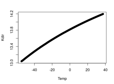
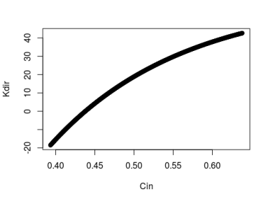
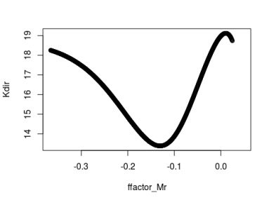
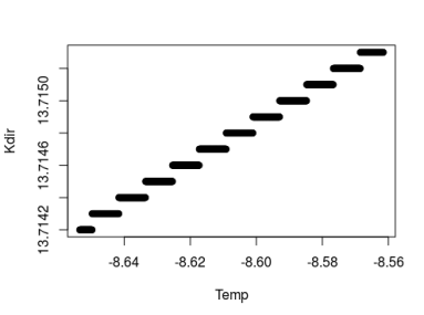
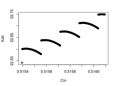
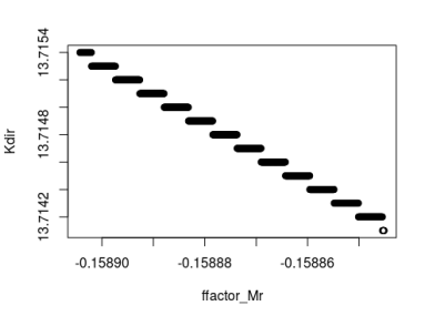
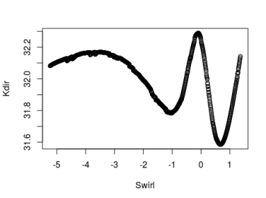
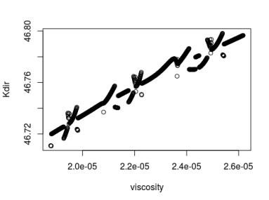
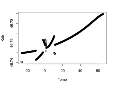
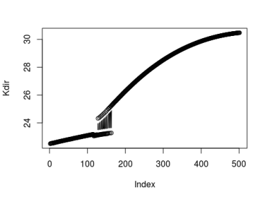
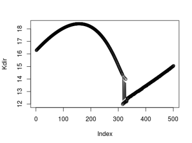
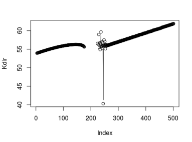
Figure 1: Local plots of ISOTSEAL response surface for direct stiffness (Kdir). Row 1: change of one input in grid in wide input ranges. Row 2: zoomed-in versions of row 1, changing one input in a much denser grid. Row 3: inexact simulations, changing one input in a grid in input space. Row 4: input trajectory between two arbitrary points from the input space, varying all inputs in grids.

Figure 1 shows example outputs $\mathbf{y}^{M}$ obtained by varying one input at a time in a narrow range, while fixing the others at sensible values (first three rows); and varying all inputs in grids between two arbitrary points (fourth row). The first row shows ideal settings: the response is a smooth function of the input over the range(s) entertained. The second row, however, zooming in on the same input–response scenarios, reveals a “staircase/striation” effect at small scales. The third row shows more concerning macro-level behavior over both narrow and wide input ranges. According to BHGE’s rotordynamics experts, these “staircase” and discontinuity features could be related to tolerances imposed on first-order equilibrium and flow equations implemented in ISOTSEAL.

The last row illustrates unpredictable regime-changing behavior and gaps due non-terminating simulation. Particular challenges exhibited by the bottom row notwithstanding, dynamics are clearly nonstationary from a global perspective. A great example of this is in the first column of the third row, where the response is at first slowly changing and then more rapidly oscillating. In that example, the regime change is smooth. In other cases, however, as in the middle column of the bottom row, a “noisy” discontinuity separates a hill-like feature from a steadier slope. An ordinary GP model, even with a nugget deployed to smooth over noiselike features by treating them as genuine noise (Gramacy and Lee,, 2012), could not accommodate such regime changes, smooth or otherwise.

Consequently, initial attempts to emulate ISOTSEAL-generated response surfaces via the canonical GP in the full (17-dimensional) input space were not successful. Even with space-filling designs sized in the several thousands, pushing the limits of the $\mathcal{O}(N^{3})$ bottleneck of large matrix decompositions, we were unable to adequately capture the distinct features we saw in smaller, more localized experiments. Modest reductions in the input dimension—holding some inputs fixed—and, similarly, reductions in the width of the input domain for the remaining coordinates led to unremarkable improvement in terms of accuracy in out-of-sample predictions. Global nonstationarity, local features, numerical artifacts, and high input dimension proved to be a perfect storm. Section 3 uses those unsuccessful proof-of-concept fits as a benchmark, showing how our proposed on-site surrogate offers a far more accurate alternative, at least from a purely out-of-sample emulation perspective.

2.2 Nonlinear least-squares calibration

To obtain a crude calibration to the small amount of field data they had, our BHGE colleagues performed a nonlinear least-squares analysis. Starting in a stable part of the input space, from the perspective of ISOTSEAL behavior, they used a numerical optimizer—a Nash variant of Marquardt NLS via QR linear solver, nlfb (Nash,, 2016)—to tune $\mathbf{u}$-values, that is, the four friction factors, based on a quadratic loss between simulated $y_{i}^{M}(\mathbf{x}_{i},\mathbf{u})$ and observed output $y_{i}^{F}(\mathbf{x}_{i})$ at the input training data sites $\mathbf{X}^{F}$.

$$\hat{\mathbf{u}}=\mathrm{arg}\min_{\mathbf{u}}\left\{\dfrac{1}{N_{F}}\sum_{i=1}^{N_{F}}\left[y^{F}_{i}(\mathbf{x}_{i})-y^{M}_{i}(\mathbf{x}_{i},\mathbf{u})\right]^{2}\right\},$$ (2)

In search for $\hat{\mathbf{u}}$, each new $\mathbf{u}$-value tried by the nlfb optimizer triggered $N_{F}$ calls to ISOTSEAL, one for each row of the design parameters $\mathbf{X}^{F}$, much in the style of Higdon et al., (2004) but without estimating a bias correction. To cope with failed ISOTSEAL runs, nlfb monitors the rate of missing values in evaluations. When the missingness rate is below a threshold (e.g., 10%), a predetermined large residual value (100 on the original scale) is imputed for the missed residual to discourage convergence toward solutions nearby. Once above the threshold, nlfb reports an error message and is started afresh.

We repeated this experiment, starting instead from 100 random space-filling $\mathbf{u}$ values in hopes of improving on our BHGE colleagues’ results with a best value at RMSE $=8.567$ and having a strong benchmark for later comparison. Because this NLS setup does not model a discrepancy between $\mathbf{y}^{M}$ and $\mathbf{y}^{F}$, converged solutions have large quadratic loss, even in-sample. Among 100 restarts, two failed; and the other losses, mapped to the scale of $\mathbf{y}^{F}$ by taking the square root, had the following distribution.

min	25%	med	mean	75%	max
6.605	8.161	8.401	10.117	9.099	25.787

The blue/circle marks in Figure 2 show observed residuals between field data and NLS calibrated ISOTSEAL with the best solution we obtained, $\hat{u}=(0.000,0.000,0.821,0.996)^{\top}$. Notice that three of four friction factors are set at their limit values. This restart benefited from a serendipitous initialization, having initial RMSE of 9.219 converging to 6.605. However, Figure 2 shows that many large residuals still remain (blue/circles).

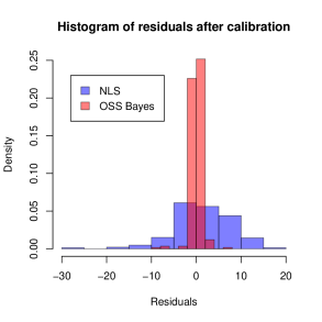
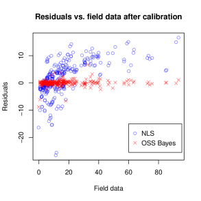
Figure 2: Observed in-sample residuals between NLS calibrated ISOTSEAL and OSS Bayes from field data. The left panel shows histograms of the residuals; the right panel shows them versus the true response. The NLS has in-sample RMSE $=6.605$. The OSS Bayes has in-sample RMSE $=1.125$, which is further discussed in Section 5.3.

The red/crosses comparator is based on our proposed methodology and is described in subsequent sections. For comparison, and to whet the reader’s appetite, we note that the in-sample RMSE we obtained was 1.125. Out-of-sample results are provided in Section 5.3. We attribute NLS’s relatively poor performance to two features. One is its inability to compensate for biases in ISOTSEAL runs, relative to the outcome of field experiments. Another is that the solutions found were highly localized to the neighborhood of the starting configuration. A post mortem analysis revealed that this was due primarily to large missingness rates.

Although we were confident that we could improve on this methodology and obtain more accurate predictions by correcting for bias between field and simulation in a Bayesian framework, it quickly became apparent that a standard, KOH-style analysis would be fraught with difficulty. In a test run, we used a space-filling design $\mathbf{X}^{M}$ and fit a global GP emulator in the 17-dimensional space of ISOTSEAL runs $\mathbf{y}^{M}$ thus obtained. That surrogate offered nice-looking predictive surfaces and provided posterior surfaces for calibrated friction factors substantially different from those obtained from NLS (e.g., away from the boundary), but unfortunately the surrogates were highly inaccurate out of sample, as illustrated below.

3 Local design and emulation for calibration

Failed attempts at surrogate modeling ISOTSEAL, either generally or for the specific purpose of calibration to field data [see Section 2.1], motivate our search for a new perspective. Local emulation has been proposed in the recent literature (Gramacy et al.,, 2015) as a means of circumventing large-data GP surrogate modeling for calibration, leveraging the important insight that surrogate evaluation is required only at field data locations $\mathbf{X}^{F}$, of which we have relatively few ($N_{F}=292$). But in that context the input dimension was small, and here we are faced with the added challenges of numerical instability, nonstationary dynamics, and missing data. In this section we port that idea to our setting of on-site surrogates, leveraging relatively cheap ISOTSEAL simulation, while mitigating problems of big $N_{M}$, big $p_{x}+p_{u}$, and challenging simulator dynamics.

3.1 On-site surrogates

On-site surrogates (OSSs) reduce a $p=p_{x}+p_{u}=17$-dimensional problem into a $p_{u}=4$-dimensional problem by building as many surrogates as there are field data observations, $N_{F}=292$. Let $\mathbf{x}$ denote a generic design variable setting and $\mathbf{u}$ a generic tuning vector (e.g., friction factor in ISOTSEAL). Then the mapping from one big surrogate to many smaller ones may be conceptualized by the following chart:

$$\hat{y}^{M}(\mathbf{x},\mathbf{u})\longrightarrow\hat{y}^{M}(\mathbf{x}_{i},\mathbf{u})\longrightarrow\hat{y}_{i}^{M}(\mathbf{u}),\quad\mbox{for }\;i=1,2,\dots,N_{F}.$$ (3)

That is, rather than building one big emulator for the entire $p$-dimensional input space $\hat{y}^{M}(\mathbf{x},\mathbf{u})$, we instead train separate emulators $\hat{y}_{i}^{M}(\mathbf{u})$ focused on each site $\mathbf{x}_{i}$ where field data has been collected. In this way, OSSs are a divide-and-conquer scheme that swap joint modeling in a large $(\mathbf{x},\mathbf{u})$-space, where design coverage and modeling fidelity could at best be thin, for many smaller models in which, separately, ample coverage is attainable with modestly sized design in $\mathbf{u}$-space only. Fitting and simulation can be performed in parallel, since the calculations for each field data site $\mathbf{x}_{i}$, $i=1,\dots,N_{F}$ are both operationally and statistically independent. Nonstationary modeling is implicit, since each surrogate focuses on a different part of the input space. If simulations are erratic for some $(\mathbf{x}_{i},\mathbf{u})$, say, the OSS indexed by $i$ can compensate by smoothing over with nonzero nuggets. If dynamics are well behaved for other sites $j$, OSSs can interpolate after the typical fashion.

In some ways, OSSs are akin to an in situ emulator (Gul et al.,, 2018). Whereas the in situ emulator is tailored to uncertainty quantification around nominal inputs, OSSs are applied in multitude for each element of $\mathbf{X}^{F}$ in the calibration setting. Another distinction is the role of design in building OSSs. Here we propose separate designs at each $\mathbf{x}_{i}$ to learn each $\hat{\mathbf{y}}_{i}^{M}(\mathbf{u})$, rather than working with design subsets. A maximin Latin hypercube sample (LHS) is preferred for their space-filling and uniform margin properties (see, e.g., Morris and Mitchell,, 1995). We use maximinLHS in the lhs (Carnell,, 2018) for R.

Specifically, at each of the $N_{F}=292$ field data sites, we create novel 1000-run maximin LHS designs for friction factors in $p_{u}=4$-dimensional $\mathbf{u}$-space. In this way, we separately design a total of $N_{M}=292,000$ ISOTSEAL simulation runs. With about one second for evaluation (for successfully terminating runs and about seven seconds waiting to terminate a failed run), this is a manageable workload requiring about 81 core-hours, or about one day on a modern hyperthreaded multicore workstation.

Let $\mathbf{y}_{i}^{M}=y^{M}(\mathbf{U}_{i})$ be a vector holding the $n_{i}$ converged ISOTSEAL runs (out of the 1,000) at the $i^{\mathrm{th}}$ site, for $i=1,\dots,N_{F}$. $\mathbf{U}_{i}$ is the corresponding $n_{i}\times p_{u}$ on-site design matrix. In our ISOTSEAL experiment, where $N_{F}=292$, a total of $N_{M}=\sum_{i=1}^{N_{F}}n_{i}=286,282$ runs terminated successfully. Most sites (241) had a complete set of $n_{i}=1000$ successful runs. Of the 51 with missing responses of varying multitudes, the smallest was $n_{238}=574$.

Each OSS comprises a fitted GP regression between successful on-site ISOTSEAL run outputs $\mathbf{y}_{i}^{M}$ and $\mathbf{U}_{i}$. Specifically, $\hat{y}_{i}^{M}(\mathbf{U}_{i})$ is built by fitting a stationary zero-mean GP using a scaled and nugget-augmented separable Gaussian power exponential kernel

$$V_{i}(\mathbf{u},\mathbf{u}^{\prime})=\tau_{i}^{2}\exp\left\{-\sum_{k=1}^{p_{u}}\frac{||\mathbf{u}_{ik}-\mathbf{u}^{\prime}_{ik}||^{2}}{\theta_{ik}}+\delta_{u,u^{\prime}}\eta_{i}\right\},$$ (4)

where $\tau_{i}^{2}$ is a site-specific scale parameter, $\mbox{\boldmath$\theta$}_{i}=(\theta_{i1},\theta_{i2},\dots,\theta_{ip_{u}})^{\top}$ is vector of site-specific lengthscales, $\eta_{i}$ is a nugget parameter, and $\delta_{u,u^{\prime}}$ is the Kronecker delta. Denote the set of hyperparameters of the $i^{\mathrm{th}}$ OSS as $\mbox{\boldmath$\phi$}_{i}=\{\tau^{2}_{i},\mbox{\boldmath$\theta$}_{i},\eta_{i}\}$, for $i=1,2,\dots,N_{F}$. Although nuggets $\eta_{i}$ are usually fit to smooth over noise, here we are including them to smooth over any deterministic numerical “jitters.” Other mean and covariance structures may be reasonable, so in what follows let $\mbox{\boldmath$\phi$}_{i}$ stand in generically for the estimable quantities of each OSS. Although numerous options for inference exist, we prefer plug-in maximum likelihood estimates (MLEs) $\hat{\mbox{\boldmath$\phi$}}_{i}$, calculated in parallel for each $i=1,\dots,N_{F}=292$ via L-BFGS-B (Byrd et al.,, 1995) using analytic derivatives via mleGPsep in the laGP package (Gramacy and Sun,, 2018; Gramacy,, 2016) for R. As we illustrate momentarily, this simple OSS strategy provides far more accurate emulation out-of-sample than does the best global alternative we could muster with a commensurate computational effort.

3.2 Merits of on-site surrogates

To build a suitable global GP competitor, we created an $N_{M}=8000$-run maximin LHS in $p=17$ input dimensions, fit a zero-mean GP based on a separable covariance structure (4), and estimated the 19-dimensional hyperparameters $\hat{\mbox{\boldmath$\phi$}}_{g}=\{\tau^{2}_{g},\mbox{\boldmath$\theta$}_{g},\eta_{g}\}$ via MLE. We chose 8,000 runs because that demanded a comparable computational effort to the OSS setup described in Section 3.1. Although the ISOTSEAL simulation effort for 8,000 runs is far less than the 292K for the OSSs, the hyperparameter inference effort and subsequent prediction for an $N_{M}=8000$-sized design is commensurate with that required for our 292 size $n_{i}\approx 1000$ OSS calculations. Repeated matrix decompositions in likelihood and derivative calculations in search of the MLE, requiring $\mathcal{O}(N_{M}^{3})$ flops for the global surrogate, represented a heavy burden even when parallelized by multi-threaded linear algebra libraries such as the Intel Math Kernel Library. Similarly threaded calculations of $O(n_{i}^{3})$ flops were faster even in 292 copies, in part because fewer evaluations were needed to learn hyperparameters $\hat{\mbox{\boldmath$\phi$}}_{i}$ in the lower-dimensional $\mathbf{u}$-space.

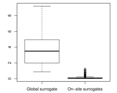
	global	OSS
min	0.871	0.008
25%	1.991	0.023
med	3.492	0.050
mean	3.619	0.120
75%	4.928	0.112
max	9.207	1.223

Figure 3: Boxplots of 292 out-of-sample RMSEs, where each RMSE is computed by using novel $n_{i}^{\prime}\leq 1,000$ on-site data from both global surrogate and OSSs.

Since the OSSs were trained on a much larger corpus of simulations, it is perhaps not surprising that they provide more accurate predictions out of sample. To demonstrate that empirically, Figure 3 summarizes the results of emulation accuracy from both global surrogate and OSSs. For our calibration goal, we need accurate emulation only at locations where we have field data $\mathbf{X}^{F}$. Therefore we entertain out-of-sample prediction accuracy only for those $\mathbf{X}^{F}$ sites. At each of the 292 field input sites $\mathbf{x}_{i}$, we design $\mathbf{U}_{i}^{\prime}$ with 1,000 runs each, the same amount as the training set, via maximin LHS. In total we collected $N_{M}^{\prime}=286,224$ testing ISOTSEAL runs, which is fewer than we ran since some came back missing. A pair of RMSEs, based on the OSSs and global surrogates, were calculated at each site $i=1,2,\dots,N_{F}=292$ based on the $n_{i}^{\prime}\approx 1,000$ testing runs located there. The distribution of these values is summarized in Figure 3. From those boxplots, one can easily see that the OSSs yield far more accurate predictions.

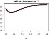
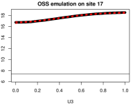
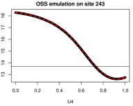
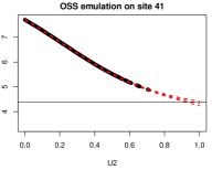
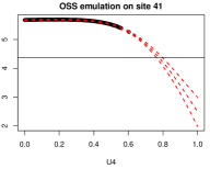
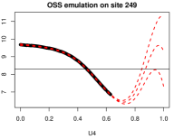
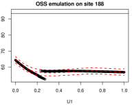
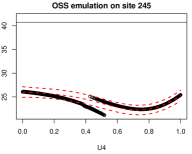
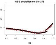
Figure 4: Profile plots of OSSs via predictive means and 95% predictive intervals (dashed-red). First row shows three well-behaved cases; middle row illustrates extrapolations to partially missing regimes; last row shows three cases where smoothing is required in order to cope with discontinuities. Red lines are the predicted mean (solid) and 95% predictive intervals (dashed). Black horizontal lines show the field response $y_{i}^{F}$ at that location, $\mathbf{x}_{i}$, with $i$ provided in the main title.

Figure 4 supplements those results with a window into the behavior of the OSSs, in three glimpses. The first row shows three relatively well-behaved input settings by varying two $\mathbf{u}$-coordinates at $\mathbf{x}_{17}^{F}$, and one at $\mathbf{x}_{243}^{F}$. In all three cases, the three dashed-red lines describing the predictive distribution (via mean, and 95% interval) completely cover the ISOTSEAL simulations in that space. Both flat (middle panel) and wavier dynamics (outer panels) are exhibited, demonstrating a degree of nonstationary flexibility. The horizontal line indicates the field data $y_{i}^{F}$ value, and in two of those cases there is a substantial discrepancy between $y^{M}(\mathbf{x}_{i},\mathbf{u})$, and $y_{i}^{F}$ for the range of $\mathbf{u}$-values on display. The middle row in the figure shows what happens when ISOTSEAL runs fail to converge, again via two $\mathbf{u}$-coordinates for one OSS, at $\mathbf{x}_{41}^{F}$, and one for another $\mathbf{x}_{249}^{F}$. Notice that failures happen more often toward the edges of $\mathbf{u}$-space, but not exclusively. In all three cases the extrapolations are sensible and reflect diversity in waviness (first two flatter, third one wavier) that could not be accommodated by a globally stationary model. All three have the corresponding $y_{i}^{F}$-value within range, but only in the extrapolated regime. The last row of the figure shows how a nugget is used to smooth over bifurcating regime changes in the output from ISOTSEAL, offering a sensible compromise and commensurately inflated uncertainty in order to cope with both regimes. All three cases map to outlying RMSE values (open circles beyond the whiskers OSS boxplot) from Figure 3. Although they are among the hardest to predict out of sample, the overall magnitude of the error is small. Since the corresponding $y_{i}^{F}$-values (horizontal lines) are far from $y^{M}(\mathbf{x}_{i},\mathbf{u})$, and $\hat{y}_{i}^{M}(\mathbf{u})$ in the $\mathbf{u}$-range under study, a substantial degree of bias correction is needed to effectively calibrate in this part of the input space.

3.3 Calibration as optimization with on-site surrogates

Even with accurate OSSs at all field data locations, Bayesian calibration can still be computationally challenging in large-scale computer experiments. In the KOH framework (1), both $\mathbf{u}^{*}$ and a bias correcting GP $b(\mathbf{x})$, via hyperparameters $\mbox{\boldmath$\phi$}_{b}$, are unknown and must jointly be estimated. The size of that parameter space, using a separable Gaussian kernel (4) for $b(\cdot)$, is large (19d) in our motivating honeycomb seal application. MCMC in such a high-dimensional space is fraught with computational challenges.

As an alternative to the fully Bayesian method, presented shortly in Section 4 taking advantage of a sparse matrix structure, and to serve as a smart initialization of the resulting MCMC scheme, we propose here an adaptation of Gramacy et al., (2015)’s modularized (Liu et al.,, 2009) calibration as optimization. Instead of sampling a full posterior distribution, $\hat{b}(\cdot)$ and $\hat{\mathbf{u}}$ are calculated as

$$\hat{\mathbf{u}}=\mathrm{arg}\max_{\mathbf{u}}\left\{p(\mathbf{u})\left[\max_{\mbox{\boldmath$\phi$}_{b}}p_{b}(\mbox{\boldmath$\phi$}_{b}\mid\mathbf{D}^{B}_{N_{F}}(\mathbf{u}))\right]\right\},$$ (5)

which explores different values of $\hat{\mathbf{u}}$ via the resulting posterior probability of discrepancy hyperparameters $p_{b}(\phi_{b}\mid\mathbf{D}^{B}_{N_{F}}(\mathbf{u}))$ applied to a data set of residuals $\mathbf{D}^{B}_{N_{F}}(\mathbf{u})$. Specifically, $\mathbf{D}^{B}_{N_{F}}(\mathbf{u})=(\mathbf{X}_{N_{F}}^{F},\hat{\mathbf{y}}_{N_{F}}^{B|u})$ is the observed field inputs $\mathbf{X}_{N_{F}}^{F}$ and discrepancies $\hat{\mathbf{y}}_{N_{F}}^{B|\mathbf{u}}=\mathbf{y}_{N_{F}}^{F}-\hat{\mathbf{y}}_{N_{F}}^{M|\mathbf{u}}$ given a particular $\mathbf{u}$. The probability $p_{b}(\cdot\mid\cdot)$ refers to the marginal likelihood of the GP with parameters $\hat{\mbox{\boldmath$\phi$}}_{b}$ fit to those residuals via their own “inner” derivative-based optimization routine. The object in Eq. (5) basically encodes the idea that $\mathbf{u}$-settings leading to better-fitting GP bias corrections are preferred. A uniform prior $p(\mathbf{u})$ is a sensible default; however, we prefer independent $u_{j}\sim\mathrm{Beta}(2,2)$ in each coordinate as a means of regularizing the search by mildly penalizing boundary solutions, in part because we know that frictions factors at the boundaries of $\mathbf{u}$-space lean heavily on the surrogate as runs of ISOTSEAL fail to converge there. Of course, any genuine prior information on $\mathbf{u}$ could be used here to further guide the calibration.

Actually, this approach is not unlike the NLS one described in Section 2.2, augmented with OSSs (rather than raw ISOTSEAL runs) and with bias correction. Instead of optimizing a least-squares criterion, our GP marginal likelihood-based loss is akin to a spatial Mahalanobis criterion (Bastos and O’Hagan,, 2009). In practice, the log of the criteria in Eq. (5) can be optimized numerically with library methods such as “L-BFGS-B”, via optim (R Core Team,, 2018), or nloptr (Ypma et al.,, 2017). Since the optimizations are fast but local and since the surface being optimized can have many local optima, we entertain a large set of random restarts—in parallel—in search for the best (most global) $\hat{\mathbf{u}}$ and $\hat{b}(\cdot)$.

To economize on space, we summarize here the outcome of this approach on the honeycomb seal, alongside its fully Bayesian KOH analog. A more detailed discussion of fully Bayesian calibration is provided in Section 4 with results in Section 5. As mentioned above, our main use of this procedure is to prime the fully Bayesian KOH MCMC. Foreshadowing somewhat, we can see from Figure 9 that the point estimates $\hat{\mathbf{u}}$ so-obtained are not much different from the maximum a posteriori (MAP) found via KOH, yet at a fraction of the computational cost. Since MCMC is inherently serial and our randomly initialized optimizations may proceed in parallel, we can get a good $\hat{\mathbf{u}}$ in about an hour, whereas getting a good (effective) sample size from the posterior takes about a day.

4 Fully Bayesian calibration via on-site surrogates

The approach in Section 3.3 is Bayesian in the sense that marginal likelihoods are used to estimate hyperparameters to the GP-based OSSs and discrepancy $b(\cdot)$, and priors are entertained for the friction factors $\mathbf{u}$. However, the modularized approach to joint modeling, via residuals from (posterior) predictive quantities paired with optimization-based point estimation, makes the setup a poor man’s Bayes at best. In the face of big data—large $N_{M}$, $N_{F}$ and $p_{u}$—such a setup may represent the only computationally tractable alternative. However, in our setting with moderate $N_{F}$ and $N_{M}=\sum_{i=1}^{N_{F}}n_{i}$ composed of independently modeled computer experiments of moderate size ($n_{i}\leq 1000$), fully Bayesian KOH-style calibration is within reach. As we show below, a careful application of partition inverse identities allows the implicit decomposition of a huge matrix via its sparse structure.

4.1 KOH setup using OSS

Our OSSs from Section 3.1 are trained via $p_{u}$-dimensional on-site designs $\mathbf{U}_{1},\mathbf{U}_{2},\dots,\mathbf{U}_{N_{F}}$. Their row dimension, $n_{i}\leq 1000$, depends on the proportion of ISOTSEAL runs that successfully completed. Collect these $N_{M}=\sum_{i=1}^{N_{F}}n_{i}$ outputs of those simulations, each tacitly paired with inputs $\mathbf{x}_{i}$, as $\mathbf{y}^{M}=(\mathbf{y}_{1},\mathbf{y}_{2},\dots,\mathbf{y}_{N_{F}})^{\top}$. The KOH framework compensates for surrogate biased computer model predictions under an unknown setting $\mathbf{u}$ by estimating a discrepancy $b(\cdot)$ via $N_{F}$ field data runs $\mathbf{y}^{F}$ observed at $N_{F}\times p_{x}$ inputs $\mathbf{X}^{F}$:

$$\mathbf{y}^{F}=y^{M}(\mathbf{U})+b(\mathbf{X}^{F}),\quad\mbox{where}\quad\mathbf{U}=[\mathbf{u}^{\top};\cdots;\mathbf{u}^{\top}]^{\top}$$

stacks $N_{F}$ identical $p_{u}$-dimensional row vectors $\mathbf{u}^{\top}$. Under joint GP priors, for each of $N_{F}$ OSSs and $b(\cdot)$, the sampling model can be characterized by the following multivariate normal (MVN) distribution.

$$\begin{bmatrix}\mathbf{y}^{M}\\ \mathbf{y}^{F}\end{bmatrix}=\begin{bmatrix}\mathbf{y}_{1}\\ \mathbf{y}_{2}\\ \vdots\\ \mathbf{y}_{N_{F}}\\ \mathbf{y}^{F}\end{bmatrix}=\begin{bmatrix}y_{1}(\mathbf{U}_{1})\\ y_{2}(\mathbf{U}_{2})\\ \vdots\\ y_{N_{F}}(\mathbf{U}_{N_{F}})\\ y^{M}(\mathbf{U})+b(\mathbf{X}^{F})\end{bmatrix}\sim\mathcal{N}_{N_{M}+N_{F}}(\mathbf{0},\mathbb{V}(\mathbf{u}))$$ (6)

Generally speaking, $\mathbb{V}(\mathbf{u})$ would be derived by hyperparameterized pairwise inverse distances between inputs on $(\mathbf{x},\mathbf{u})$-space. In our OSS setup, however, it has a special structure owing to the independent surrogates fit at each $\mathbf{x}_{i}$, for $i=1,\dots,N_{F}$.

Let $\mathbf{V}_{i}\equiv V_{i}(\mathbf{U}_{i},\mathbf{U}_{i})$ denote the $n_{i}\times n_{i}$ covariance matrix for the $i^{\mathrm{th}}$ OSS, for example, following Eq. (4). This notation deliberately suppresses dependence on hyperparameters $\mbox{\boldmath$\phi$}_{i}$, which is a topic we table momentarily to streamline the discussion here. Similarly, $V_{b}\equiv V_{b}(\mathbf{X}^{F})$. Let $V_{i}(\mathbf{U})\equiv V_{i}(\mathbf{U},\mathbf{U}_{i})$ be the $n_{i}\times N_{F}$ matrix of the $i^{\mathrm{th}}$ OSS’s cross-covariances between field data locations, paired with $\mathbf{u}$-values, and $(\mathbf{x}_{i},\mathbf{U}_{i})$ design locations. Since the $i^{\mathrm{th}}$ OSS is tailored to $\mathbf{x}_{i}$ only, independent of the other $\mathbf{X}^{F}$, this matrix is zero except in the $i^{\mathrm{th}}$ row. Let $\mathbf{v}\mathbb{I}_{N_{F}}$ be a $N_{F}\times N_{F}$ diagonal matrix holding $V_{i}(\mathbf{u}^{\prime},\mathbf{u}^{\prime})$ values. Although expressed as a function of $\mathbf{u}^{\prime}$ it is not actually a function of $\mathbf{u}^{\prime}$ because the distance between $\mathbf{u}^{\prime}$ and itself is zero. Using Eq. (4) would yield $\mathbf{v}\mathbb{I}_{N_{F}}=\mathrm{Diag}[\tau_{i}^{2}(1+\eta_{i})]$. With those definitions, we have the following:

$$\mathbb{V}(\mathbf{u})=\begin{bmatrix}\mathbf{V}_{1}&\mathbf{0}&\mathbf{0}&\mathbf{0}&V_{1}(\mathbf{U})^{\top}\\ \mathbf{0}&\mathbf{V}_{2}&\mathbf{0}&\mathbf{0}&V_{2}(\mathbf{U})^{\top}\\ \mathbf{0}&\mathbf{0}&\ddots&\mathbf{0}&\vdots\\ \mathbf{0}&\mathbf{0}&\mathbf{0}&\mathbf{V}_{N_{F}}&V_{N_{F}}(\mathbf{U})^{\top}\\ V_{1}(\mathbf{U})&V_{2}(\mathbf{U})&\dots&V_{N_{F}}(\mathbf{U})&\mathbf{v}\mathbb{I}_{N_{F}}+V_{b}(\mathbf{X}^{F})\end{bmatrix}\equiv\begin{bmatrix}\mathbb{V}_{o}&\mathbb{V}^{\top}_{ob}(\mathbf{u})\\ \mathbb{V}_{ob}(\mathbf{u})&\mathbb{V}_{b}\end{bmatrix}.$$ (7)

Although $\mathbb{V}(\mathbf{u})$ is huge, being $(N_{M}+N_{F})\times(N_{M}+N_{F})$ or roughly $292292\times 292292>85$ billion entries in our honeycomb setup, it is sparse, having several orders of magnitude fewer nonzero entries—about 292 million in our setup. That is still too big, even for sparse matrix manipulation. Fortunately, the block diagonal structure makes it possible to work with, via more conventional libraries. Toward that end, denote by $\mathbb{V}_{o}=\operatorname{Diag}[\mathbf{V}_{i}(\mathbf{U}_{i},\mathbf{U}_{i})]$ the huge $N_{F}\cdot(n_{i}\times n_{i})$ upper-left block diagonal submatrix from the OSSs. Let $\mathbb{V}_{b}=\mathbf{v}\mathbb{I}_{N_{F}}+V_{b}(\mathbf{X}^{F})$ represent the remaining (dense) lower-right block, corresponding to the bias. Abstract by $\mathbb{V}_{ob}(\mathbf{u})$ and $V_{ob}^{\top}(\mathbf{u})$ the remaining, symmetric, rows and columns on the edges. Recall that the $V_{i}(\mathbf{U})$ therein are themselves sparse, comprising a single row of nonzero entries.

Before detailing in Section 4.2 how we use these blocks, first focus on the specific operations required. A fully Bayesian approach to inference for $\mathbf{u}$ via posterior $p(\mathbf{u}\mid\mathbf{y}^{M},\mathbf{y}^{F})\propto p(\mathbf{y}^{M},\mathbf{y}^{F}\mid\mathbf{u})\cdot p(\mathbf{u})$ involves evaluating an MVN likelihood

$$p(\mathbf{y}^{M},\mathbf{y}^{F}\mid\mathbf{u})\propto|\mathbb{V}(\mathbf{u})|^{-\frac{1}{2}}\times\exp\left\{-\dfrac{1}{2}\begin{bmatrix}\mathbf{y}^{M}\\ \mathbf{y}^{F}\end{bmatrix}^{\top}\mathbb{V}^{-1}(\mathbf{u})\begin{bmatrix}\mathbf{y}^{M}\\ \mathbf{y}^{F}\end{bmatrix}\right\}.$$ (8)

The main computational challenges are manifest in the inverse $\mathbb{V}^{-1}(\mathbf{u})$ and determinant $|\mathbb{V}(\mathbf{u})|$ calculations, both involving $\mathcal{O}((N_{M}+N_{F})^{3})$ flops in addition to $\mathcal{O}((N_{M}+N_{F})^{2})$ storage, assuming a dense representation. However, substantial savings comes from the sparse structure (7) of $\mathbb{V}(\mathbf{u})$ and that only a portion—the edges—involves $\mathbf{u}$.

4.2 On-site surrogate decomposition

Partition inverse and determinant equations (e.g., Petersen et al.,, 2008) provide convenient forms for the requisite decompositions of $\mathbb{V}(\mathbf{u})$:

$$\mathbb{V}^{-1}(\mathbf{u}) =\begin{bmatrix}\mathbb{V}_{o}&\mathbb{V}_{ob}^{\top}(\mathbf{u})\\ \mathbb{V}_{ob}(\mathbf{u})&\mathbb{V}_{b}\end{bmatrix}^{-1}\!\!\!\!\!\!=\begin{bmatrix}\mathbb{V}_{o}^{-1}+\mathbb{V}_{o}^{-1}\mathbb{V}_{ob}^{\top}(\mathbf{u})\mathbb{C}^{-1}(\mathbf{u})\mathbb{V}_{ob}(\mathbf{u})\mathbb{V}_{o}^{-1}&-\mathbb{V}_{o}^{-1}\mathbb{V}_{ob}^{\top}(\mathbf{u})\mathbb{C}^{-1}(\mathbf{u})\\ -\mathbb{C}^{-1}(\mathbf{u})\mathbb{V}_{ob}(\mathbf{u})\mathbb{V}_{o}^{-1}&\mathbb{C}^{-1}(\mathbf{u})\end{bmatrix}$$

$$|\mathbb{V}(\mathbf{u})| =\det\begin{bmatrix}\mathbb{V}_{o}&\mathbb{V}_{ob}^{\top}(\mathbf{u})\\ \mathbb{V}_{ob}(\mathbf{u})&\mathbb{V}_{b}\end{bmatrix}=\det(\mathbb{V}_{o})\times\det(\mathbb{C(\mathbf{u})}),$$ (9)

where $\mathbb{C}(\mathbf{u})=\mathbb{V}_{b}-\mathbb{V}_{ob}(\mathbf{u})\mathbb{V}_{o}^{-1}\mathbb{V}_{ob}^{\top}(\mathbf{u})$. Eq. (9) involves a potentially huge $N_{M}\times N_{M}$ component $\mathbb{V}_{o}$, with $N_{M}=286,282$ in the honeycomb example. Since it is block diagonal, thanks to the OSS structure, we have

$$\mathbb{V}_{o}^{-1}=\operatorname{Diag}[\mathbf{V}_{i}^{-1}]\quad\mbox{ and }\quad\det(\mathbb{V}_{o})=\prod_{i=1}^{N_{F}}\det[\mathbf{V}_{i}].$$ (10)

In this way, an otherwise $\mathcal{O}(N_{M}^{3})$ operation may instead by calculated via $N_{F}\times\mathcal{O}(n_{i}^{3})$ calculations, potentially in parallel. If some $n_{i}$ are big, then the burden could still be substantial. However, both are constant with respect to $\mathbf{u}$, so only one such decomposition is required, even when entertaining thousands of potential $\mathbf{u}$. With $n_{i}\leq 1000$ in our honeycomb application, these calculations require mere seconds, even in serial.

Similar tricks extend to other quantities involved in Eq. (9). Consider $\mathbb{V}_{o}^{-1}\mathbb{V}_{ob}^{\top}(\mathbf{u})$, which appears multiple times in original and transposed forms. We have

$$\mathbb{V}_{o}^{-1}\mathbb{V}_{ob}^{\top}(\mathbf{u})=\operatorname{Diag}[\mathbf{V}_{i}^{-1}V_{i}(\mathbf{U})]=\operatorname{Diag}[\mathbf{h}_{i}(\mathbf{u})]\quad\mbox{where}\quad\mathbf{h}_{i}(\mathbf{u})=\mathbf{V}_{i}^{-1}V_{i}(\mathbf{u}),$$ (11)

and $V_{i}(\mathbf{u})$ is a vector holding the nonzero part of $V_{i}(\mathbf{U})$. In other words, $\mathbb{V}_{o}^{-1}\mathbb{V}_{ob}^{\top}(\mathbf{u})$ is a $N_{M}\times N_{F}$ matrix comprising $N_{F}$ column vectors, whose $n_{i}$ nonzero entries $\mathbf{h}_{i}$ follow a block structure for columns $i=1,\dots N_{F}$. Each $\mathbf{h}_{i}(\mathbf{u})$ can be updated in parallel for new $\mathbf{u}$.

Next consider $\mathbb{C}(\mathbf{u})=\mathbb{V}_{b}-\mathbb{V}_{ob}(\mathbf{u})\mathbb{V}_{o}^{-1}\mathbb{V}_{ob}^{\top}(\mathbf{u})$, which appears in each block of Eq. (9). $\mathbb{C}(\mathbf{u})$ is dense but is easy to compute because it is just $N_{F}\times N_{F}$. Recall from Eq .7 that $\mathbb{V}_{b}=\mathbf{v}\mathbb{I}_{N_{F}}+{V}_{b}(\mathbf{X}^{F})$, which requires inversion only once because it is constant in $\mathbf{u}$. The next part $\mathbb{V}_{ob}(\mathbf{u})\mathbb{V}_{o}^{-1}\mathbb{V}_{ob}^{\top}(\mathbf{u})$ extends nicely from $\mathbb{V}_{o}^{-1}\mathbb{V}_{ob}^{\top}(\mathbf{u})=\mathrm{Diag}[V_{i}(\mathbf{u})^{\top}\mathbf{h}_{i}(\mathbf{u})]$ following Eq. (11), an $N_{F}\times N_{F}$ diagonal matrix whose entries can be calculated alongside the $\mathbf{h}_{i}(\mathbf{u})$, similarly parallelized over $i=1,\dots,N_{F}$.

Combining $\mathbb{V}_{o}^{-1}\mathbb{V}_{ob}^{\top}(\mathbf{u})$ and $\mathbb{C}(\mathbf{u})$ results gives $\mathbb{V}_{o}^{-1}\mathbb{V}_{ob}^{\top}(\mathbf{u})\mathbb{C}^{-1}(\mathbf{u})=\mathbf{H}(\mathbf{u})\circ\mathbb{C}^{-1}(\mathbf{u})$, where “$\circ$” is the Hadamard product applied columnwise to $\mathbb{C}^{-1}(\mathbf{u})$ and where $\mathbf{H}(\mathbf{u})=[\mathbf{h}_{1}(\mathbf{u});\dots;\mathbf{h}_{N_{F}}(\mathbf{u})]$. More concretely,

$$\mathbb{V}_{o}^{-1}\mathbb{V}_{ob}^{\top}(\mathbf{u})\mathbb{C}^{-1}(\mathbf{u})=\begin{bmatrix}c_{1,1}\mathbf{h}_{1}(\mathbf{u})&c_{1,2}\mathbf{h}_{1}(\mathbf{u})&\dots&c_{1,N_{F}}\mathbf{h}_{1}(\mathbf{u})\\ c_{2,1}\mathbf{h}_{2}(\mathbf{u})&c_{2,2}\mathbf{h}_{2}(\mathbf{u})&\dots&c_{2,N_{F}}\mathbf{h}_{2}(\mathbf{u})\\ \vdots&\vdots&\ddots&\vdots\\ c_{N_{F},1}\mathbf{h}_{N_{F}}(\mathbf{u})&c_{N_{F},2}\mathbf{h}_{N_{F}}(\mathbf{u})&\dots&c_{N_{F},N_{F}}\mathbf{h}_{N_{F}}(\mathbf{u})\end{bmatrix},$$

where $c_{i,j}$ are scalar elements of $\mathbb{C}^{-1}(\mathbf{u})$.

Returning to Eq. (9), combining with Eq. (10), establishes the determinant analog.

$$|\mathbb{V}(\mathbf{u})|=\det(\mathbb{V}_{o})\times\det(\mathbb{C}(\mathbf{u}))=\prod_{i=1}^{N_{F}}\det[\mathbf{V}_{i}]\times\det(\mathbb{C}(\mathbf{u}))$$ (12)

The first component, $\prod_{i=1}^{N_{F}}\det[\mathbf{V}_{i}(\mathbf{U}_{i},\mathbf{U}_{i})]$, is composed of $\mathcal{O}(n_{i}^{3})$ computations, constant in $\mathbf{u}$. Only the second component, $\det(\mathbb{C}(\mathbf{u}))$ needs to be updated with new $\mathbf{u}$.

In summary, OSSs can be exploited to circumvent huge matrix computations involved in likelihood evaluation (8), yielding a structure benefiting from a degree of precalculation, and from parallelization if desired. These features come on top of largely improved emulation accuracy demonstrated in Section 3.2, compared with the global alternative.

4.3 Priors and computation

As briefly described in Section 3.3, we consider two priors on $\mathbf{u}$, the friction factors in our honeycomb example. The first is independent uniform, $u_{j}\stackrel{{\scriptstyle\mathrm{iid}}}{{\sim}}\mathrm{Unif}(0,1)$. The second is $u_{j}\stackrel{{\scriptstyle\mathrm{iid}}}{{\sim}}\mathrm{Beta}(2,2)$ as a means of regularizing posterior inference. The marginal posterior for $\mathbf{u}$ is known to sometimes concentrate on the boundaries $\mathbf{u}$-space, because of identifiability challenges in the KOH framework (see, e.g., Gramacy et al.,, 2015). Furthermore, we know that ISOTSEAL is least stable in that region. $\mathrm{Beta}(2,2)$ slightly discourages that boundary and commensurately elevates the posterior density of central values. This choice has the added benefit of providing better mixing in the MCMC described momentarily.

The coupled GPs involved in the KOH setup are hyperparameterized by scales, lengthscales, and nuggets as in Eq. (4). A fully Bayesian analysis would include these in the parameter space for posterior sampling, augmenting the dimension by an order of magnitude in many cases. In other words, the posterior becomes $p(\mathbf{u},\mathbf{\Phi}\mid\mathbf{y}^{M},\mathbf{y}^{F})$, where $|\Phi|\in\mathcal{O}(p+p_{x})$, $p=p_{x}+p_{u}$ for surrogate and $p_{x}$ for discrepancy, which would work out to more than thirty parameters in our honeycomb example. Because of that high dimensionality, a common simplifying tactic is to fix those $\mathbf{\Phi}$ at their MLE or MAP setting $\hat{\mathbf{\Phi}}$, found via numerical optimization. In our OSS setup, with $N_{F}=292$ independent surrogates, the burden of hyperparameterization is exacerbated, with $|\Phi|\in\mathcal{O}(N_{F}p_{u}+p_{x})$ being several orders of magnitude higher in dimension, over one thousand for honeycomb. This all but demands a setup where point estimates are first obtained via maximization, as in Section 3.3. That leaves only $\mathbf{u}$ for posterior sampling via $p(\mathbf{u}\mid\mathbf{y}^{M},\mathbf{y}^{F},\hat{\mathbf{\Phi}})$. Additionally, we initialize our Monte Carlo search of the posterior with $\hat{\mathbf{u}}$ values found via Section 3.3.

Following KOH, we employ MCMC (Hastings,, 1970; Gelfand and Smith,, 1990) to sample from the posterior in a Metropolis-within-Gibbs fashion (see, e.g., Hoff,, 2009). Each Gibbs step utilizes a marginal random-walk Gaussian proposal $u_{j}^{\prime}=u_{j}+s_{j}$, $s_{j}\stackrel{{\scriptstyle\mathrm{iid}}}{{\sim}}\mathcal{N}(0,\sigma_{j}^{2})$, $j=1,\dots,p_{u}$. A pilot tuning stage was used to tune the $\sigma_{j}$, leading to $\sigma=(0.02,0.01,0.2,0.1)^{\top}$ in the honeycomb example. Figures 8–9 in Section 5.2 indicate good mixing and adequate posterior exploration of the four-dimensional space of friction factors.

5 Empirical results

Before detailing the outcome of this setup on our motivating honeycomb example, we illustrate the methodology in a more controlled setting.

5.1 Illustrative example

Consider a mathematical model $y^{M^{*}}(\cdot)$ with three inputs $(x,u_{1},u_{2})$, following

$$y^{M^{*}}(x,u_{1},u_{2})=\cos\left(\dfrac{25\sin(x)\times x\times u_{1}}{x+u_{2}}\right),$$ (13)

where $x\in[0,1]$ is a one-dimensional field input and $\mathbf{u}=(u_{1},u_{2})\in[0,1]^{2}$ are two-dimensional calibration parameters. Suppose the real process follows

$$y^{R}(x)=y^{M^{*}}(x,0.8,0.2)+b(x)\quad\mbox{where}\quad b(x)=\sin(4x).$$

Mimicking the features of ISOTSEAL, suppose the computer model $y^{M}$ is unreliable in its evaluation of the mathematical model $y^{M^{*}}$, sometimes returning NA values. Specifically, suppose the response is missing when the $\mathbf{u}$ input is in its upper quartile, $u1\times u2>0.5$, and $[5y^{M^{*}}]\mod 2\equiv 0$, where $[\cdot]$ rounds to the nearest integer. Figure 5 provides an illustration.

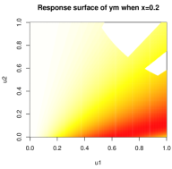
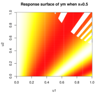
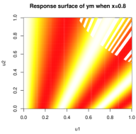
Figure 5: Response surfaces illustrating computer model following (13) with missing values under three settings of $x$.

Each panel in the figure shows the response as a function of $(u_{1},u_{2})$ for a different setting of $x$. Observe the nonstationary dynamics manifest in increasing waviness of the surface as $x$ increases. Similarly, the pattern of missingness becomes more complex for increasing $x$. Therefore, a global surrogate would struggle on two fronts: with stationarity as well as with (nonmissing) coverage of the design in $\mathbf{u}$-space.

Now consider observing $N_{F}$ field realizations of $y^{R}(x)+\varepsilon$, where $\varepsilon\sim\mathcal{N}(0,0.02^{2})$, under a maximin LHS in $x$-space, and two variations on a computer experiment toward a calibrated model. The first involves a global GP surrogate fit to $N_{M}=500$ computer model evaluations via a maximin LHS in $(x,\mathbf{u})$-space, where 33 (6.6%) came back NA. The second uses OSSs trained on $n_{i}=200$ maximin LHSs in $\mathbf{u}$-space, paired with $x_{i}^{F}$ for $i=1,\dots,N_{F}$. Of the $N_{M}=2,000$ such simulations, 95 came back missing (4.75%). The sizes of these computer experiment designs were chosen so that the computing demands required for the global and OSS surrogates were commensurate. Counting flops, the global approach requires about $500^{3}=1.25\times 10^{8}$, whereas the OSSs need $10\times 200^{3}=8\times 10^{7}$, which can be 10-fold parallelized if desired.

Before turning to calibration, consider first the accuracy of the two surrogates. Mirroring Figure 3 for ISOTSEAL in our honeycomb example, Figure 6 shows the result of an out-of-sample comparison of otherwise identical design.

	global	OSS
min	0.0472	0.0004
25%	0.1090	0.0012
med	0.1357	0.0039
mean	0.1398	0.0052
75%	0.1673	0.0090
max	0.2403	0.0124

Figure 6: Boxplots of 10 out-of-sample RMSEs, where each RMSE is computed by using novel $n_{i}^{\prime}\leq 200$, for $i=1,\dots,N_{F}$.

The story here is similar to the one for ISOTSEAL. Clearly, the OSSs are more accurate. They are better able to capture the nonstationarity nature of computer model $y^{M}(\cdot,\cdot)$ nearby to the field sites.

Next, we compare calibration results from global surrogate optimization, OSSs via modularization/optimization [Section 3.3, and OSSs via full Bayes [Section 4]. In this simple toy example, uniform priors $u_{i}\stackrel{{\scriptstyle\mathrm{iid}}}{{\sim}}\mathrm{Unif}(0,1)$ are sufficient for good performance. The first row of Figure 7 shows the distributions of converged $\hat{\mathbf{u}}$ via Eq. (5) from the optimization approach described in Section 3.3. The left panel corresponds to the lower-fidelity global surrogate and the right panel to the higher-fidelity OSSs. Converged solutions from 500 random initializations are shown. Terrain colors on the ranked log posteriors are provided to aid in visualization. The best single coordinate $\hat{\mathbf{u}}$ is indicated by the black dot. For comparison, the true $\mathbf{u}^{*}$ value is shown as red-dashed crosshairs. Although the best $\hat{\mathbf{u}}$ values found cluster near the truth, both are sometimes fooled by a posterior ridge in another quadrant of the space.

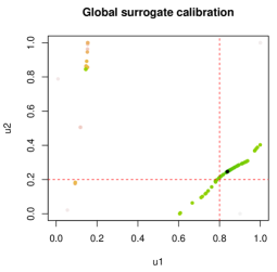
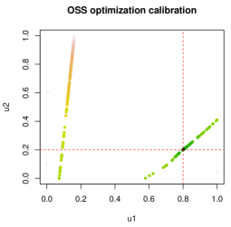
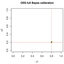
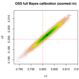
Figure 7: Calibration results from optimization and full Bayes for the toy example. Terrain colors are derived from ranks of log-scaled posteriors as a visual aid; black dots indicate the MAP setting; red dashed lines are the true values of calibration parameters, $\hat{\mathbf{u}}$.

The second row of Figure 7 shows the posterior distribution of $\mathbf{u}$ in full (left) and zoomed-in ranges (right). Compared with the OSS-based optimization approach, the KOH analog found $\mathbf{u}$’s tightly coupled around the truth.

In this simple example, posterior uncertainty is low, in part because a relatively large computer experiment could be entertained in a small input dimension. In fact all three methods worked reasonably well. However, as we entertain more realistic settings, such as the honeycomb in 17 dimensions, only the methods based on OSSs are viable computationally (assuming a relatively dense sampling of the computer model is viable).

5.2 KOH versus modularized optimization: on honeycomb

Here we return to our motivating honeycomb seal example, first providing a qualitative comparison between our two approaches based on OSSs, via modularized optimization [Section 3.3] and KOH [Section 4]. We then turn to an out-of-sample comparison, pitting the KOH framework against the initial NLS analysis. Throughout, we use a regularizing independent $\mathrm{Beta}(2,2)$ prior on the components of $\mathbf{u}$. Appendix 7 provides an analog presentation under a uniform prior, accompanied by a brief discussion.

Figure 8 shows traces of the samples obtained via our Metropolis-within-Gibbs scheme, described in Section 4.3.

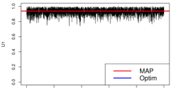
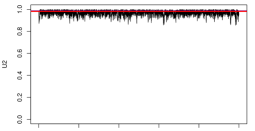
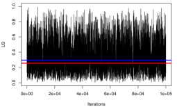
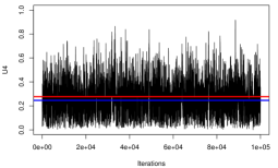
Figure 8: Trace plots of MCMC samples for all calibration parameters $\mathbf{u}$ after burn-in. Blue line indicates the best setting for $\mathbf{u}$ from optimization. Red line indicates the MAP $\mathbf{u}$ extracted from the samples; modular/opt added for comparison.

The figure indicates clear convergence to the stationary distribution with mixing that is qualitatively quite good. The effective sample sizes (ESS) (Kass et al.,, 1998), marginally for all four friction factors, are sufficiently high at $\mathrm{ESS}_{u_{1}}=1026$, $\mathrm{ESS}_{u_{2}}=684$, $\mathrm{ESS}_{u_{3}}=2062$, $\mathrm{ESS}_{u_{4}}=1462$, respectively.

Figure 8 clearly shows that the posterior is, at least marginally, far more concentrated for the first two friction factors (first row) than for the last two. For a better joint glimpse at the four-dimensional posterior distribution of $\mathbf{u}$, the bottom-left panels of Figure 9 show these samples via pairs of coordinates. The points are colored by a rank-transformed log-scaled posterior evaluation as a means of better visualizing the high concentrations in a cramped space. Histograms along the diagonal panels show individual margins; panels on the top-right mirror those on the bottom-left but instead show solutions found by the modular/optimal approach [Section 3.3] in 500 random restarts.

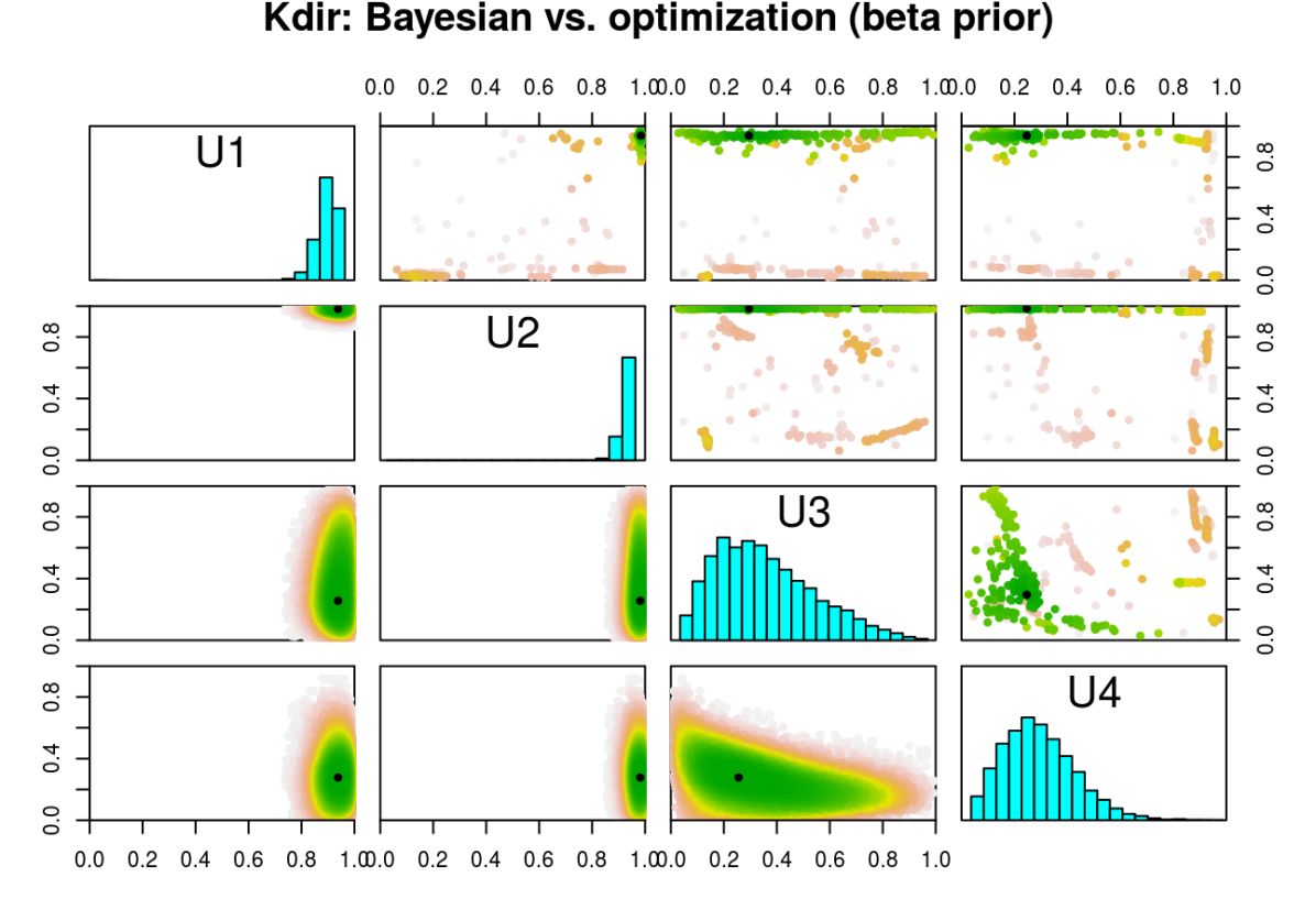
Figure 9: Bayesian KOH (lower and diagonal) posterior for $\mathbf{u}$ vs. modularlized optimization (upper) analog, both under an independent $\mathrm{Beta}(2,2)$ prior for $\mathbf{u}$. Colors are derived from ranks of posterior probabilities to aid in visualization. Modularized results are from 500 converged optimization under random initialization. Black dots indicate MAP values.

Several notable observations can be drawn from the plots in that figure. For one, consistency is high between the two approaches: KOH and modular/opt. Although the values of log posteriors evaluations are not directly comparable across the models, both agree on most probable values (black dots in the off-diagonal panels). A diversity of solutions from the optimization-based approach indicates that the solver struggles to navigate the log posterior surface but usually finds estimates that are in the right ballpark. The full posterior distribution via KOH indicates that the first two friction factors are well pinned-down by the posterior. However, posterior concentration is more diffuse for the latter two. A complicated correlation structure is evident in $(u_{3},u_{4})$.

A similar suite of results under an independent uniform prior is provided in Appendix 7. The story there is similar, except that the posterior sampling concentrates more heavily on the boundary of $\mathbf{u}$-space for all four parameters. Considering that we know our ISOTSEAL simulator is less reliable in those regimes, leading to far more missing values and thus requiring greater degree of extrapolation from our OSSs, we prefer the more stable regime (better emulation and MCMC mixing) offered by light penalization under a $\mathrm{Beta}(2,2)$ prior.

5.3 Out-of-sample prediction

To close the loop on our NLS comparison from Section 2.2, particularly Figure 2 highlighting in-sample prediction, we conclude our empirical work on the honeycomb with an exercise measuring out-of-sample predictive accuracy. Pointwise comparators based on several variations are entertained, e.g., with/without OSSs, with/without estimated discrepancies compensating for bias. Finally, we complete the Bayesian KOH OSS setup (Section 4) with a predictor that tractably propagates uncertainty through the sparse covariance structure.

The NLS baseline from Section 2.2 involves direct application of ISOTSEAL for new physical (testing) site $\mathbf{x}_{\mathrm{\mathrm{new}}}$, paired with plug-in $\hat{\mathbf{u}}$ furnished by our BHGE colleagues:

$$\hat{y}^{F}(\mathbf{x}_{\mathrm{\mathrm{new}}})={y}^{M}(\mathbf{x}_{\mathrm{\mathrm{new}}},\hat{\mathbf{u}}^{\text{NLS}})$$ (14)

No bias correction is applied. Figure 10, augmenting Figure 2, provides a view into residuals under this comparator, and others explained momentarily. We clarify that these NLS results are ”in-sample” as they use the same data our BHGE colleagues trained on. Precise root mean-squared errors (RMSEs) and $\hat{\mathbf{u}}$-values are summarized in Table 1.

Feeding $\hat{\mathbf{u}}$ directly into ISOTSEAL is problematic because simulation dynamics are nonstationary, unstable, and unreliable. We had trouble getting an implementation of this variation to behave reliably enough in order to report meaningful out-of-sample results. As demonstrated in Section 2.1, and the second row in Figure 4, ISOTSEAL can fail to converge and instead return ${y}^{M}(\mathbf{x}_{\mathrm{\mathrm{new}}},\hat{\mathbf{u}})=$ NA especially at $\mathbf{u}$ around the upper limit of their range(s). Our BHGE colleagues carefully engineered their NLS search to avoid problematic $\mathbf{u}$-settings. OSSs were proposed in order to more gracefully cope with NAs and to correct for other idiosyncrasies. When predicting out of sample, a new OSS $\hat{y}^{M}(\mathbf{x}_{\mathrm{\mathrm{new}}},\cdot)$ must be fit via new on-site design $\mathbf{U}_{\mathrm{\mathrm{new}}}$ paired with $\mathbf{x}_{\mathrm{\mathrm{new}}}$. As with OSS training described in Section 3.1, we shall utilize a size $n=1000$ maximin LHS.

Surrogate $\hat{y}^{M}(.,.)$ enables a full search of the entire $\mathbf{u}$-space, offering the potential of finding a better $\hat{\mathbf{u}}$ especially nearby regions where direct ISOTSEAL runs may fail. Acting on OSSs without discrepancy correction, we find $\hat{\mathbf{u}}^{\text{OSS}}_{\text{nobias}}$ slightly different from the $\hat{\mathbf{u}}^{\text{NLS}}$ using direct ISOTSEAL runs. See Table 1. To compare the predictive performance directly to the in-sample NLS, we plug-in $\hat{\mathbf{u}}^{\text{OSS}}_{\text{nobias}}$ for new site $\mathbf{x}_{\mathrm{\mathrm{new}}}$ though the new OSS:

$$\hat{y}^{F}(\mathbf{x}_{\mathrm{\mathrm{new}}})=\hat{y}^{M}(\mathbf{x}_{\mathrm{\mathrm{new}}},\hat{\mathbf{u}}^{\text{OSS}}_{\text{nobias}}).$$ (15)

Figure 10 indicates similar residual behavior for these two comparators. OSSs without bias correction fares slightly worse than the NLS analog, however note that the latter is truly out-of-sample and the former was technically in-sample. The OSS version $\hat{y}^{M}(\mathbf{x}_{\mathrm{\mathrm{new}}},\hat{\mathbf{u}}^{\text{OSS}}_{\text{nobias}})$ offers fuller uncertainty quantification in predictions, via local GP predictive variances.

Now consider variations which correct for potential bias between OSS and field data measurements. Feed $\hat{\mathbf{u}}$ through the OSS and obtain

$$\hat{y}^{F}(\mathbf{x}_{\mathrm{\mathrm{new}}})=\hat{y}^{M}(\mathbf{x}_{\mathrm{\mathrm{new}}},\hat{\mathbf{u}})+\hat{b}(\mathbf{x}_{\mathrm{\mathrm{new}}})$$ (16)

To benchmark these predictions out of sample we designed the following leave-one-out (LOO) cross-validation (CV) experiment. Alternately excluding each field data location $i=1,\dots,N_{F}=292$, we fit 292 LOO discrepancy terms $\hat{b}^{(-i)}(\cdot)$ via residuals $\mathbf{y}^{F}_{(-i)}-\hat{\mathbf{y}}^{M}_{(-i)}$ and $\mathbf{X}^{F}_{(-i)}$. We could build a new OSS for $\mathbf{x}_{i}$, treating it as a $\mathbf{x}_{\mathrm{\mathrm{new}}}$ as described above, but instead it is equivalent (and computationally more thrifty) to use the $\mathbf{U}_{i}$ we already have. Based on those calculations, point predictions are composed of

$$\hat{y}^{F}({\mathbf{x}_{i}})=\hat{y}^{M}(\mathbf{x}_{i},\hat{\mathbf{u}})+\hat{b}^{(-i)}(\mathbf{x}_{i}),\quad\mbox{for}\quad i=1,2,\dots,N_{F}.$$ (17)

Predictions thus obtained are compared with true outputs $\mathbf{y}^{F}$ and residuals for RMSE calculations. We note that this experiment focuses primarily on bias correction. New $\hat{\mathbf{u}}_{(-i)}$ are not calculated for each of $i=1,\dots,N_{F}$ due to the prohibitive computational cost.

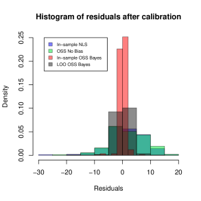
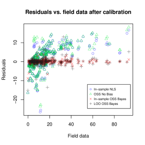
Figure 10: Residuals to honeycomb field data. The left panel shows histograms comparing three approaches; the right panel plots them versus the true response.

Figure 10 shows those LOO residuals graphically alongside our other comparators. Only results for $\hat{\mathbf{u}}$ via modular/opt framework are shown here since $\hat{\mathbf{u}}$ from the fully Bayes KOH setup are similar. The panels in the figure indicate that bias correction offers substantial improvement over NLS: in-sample NLS residuals are worse than LOO OSS Bayes results. Summarizing those residuals, modular/opt calibration with discrepancy has an leave-one-out RMSE of $2.126$, being even smaller than both the in-sample NLS value of $6.605$ reported in Section 2.2 and the in-sample OSS no-bias value of $6.818$. Furthermore, LOO OSS modular/opt RMSE is comparable to its in-sample analog of $1.125$.

Method	$\hat{u}_{1}$	$\hat{u}_{2}$	$\hat{u}_{3}$	$\hat{u}_{4}$	RMSE
In-sample NLS	0.00000	0.00000	0.82123	0.99615	6.605
OSS No Bias	0.00877	0.17352	0.94893	0.94474	6.818
In-sample OSS Bayes	0.93659	0.98348	0.28441	0.25975	1.125
LOO OSS modular/opt	0.93659	0.98348	0.28441	0.25975	2.126
LOO OSS KOH full Bayes	0.93659	0.98348	0.28441	0.25975	1.957

Table 1: Estimated $\hat{\mathbf{u}}$ and RMSEs from in-sample and LOO comparisons.

Next we develop fully Bayesian prediction for $y^{F}(\mathbf{X}^{F}_{\mathrm{new}})$ at $N^{\prime}_{F}$ new physical locations $\mathbf{X}^{F}_{\mathrm{new}}=(\mathbf{x}^{\mathrm{new}}_{1},\mathbf{x}^{\mathrm{new}}_{2},\dots,\mathbf{x}^{\mathrm{new}}_{N^{\prime}_{F}})^{\top}$. As in the pointwise case, $N^{\prime}_{F}$ new OSSs must be built on $N^{\prime}_{M}$ new on-site simulations $\mathbf{y}^{M}_{\mathrm{new}}=(\mathbf{y}_{N_{F}+1},\dots,\mathbf{y}_{N_{F}+N^{\prime}_{F}})^{\top}$. Following from Eq. (8),

$$\begin{bmatrix}\mathbf{y}^{M}\\ \mathbf{y}^{F}\\ \mathbf{y}^{M}_{\mathrm{new}}\\ \mathbf{y}^{F}_{\mathrm{new}}\end{bmatrix}=\begin{bmatrix}\mathbf{y}_{1}\\ \vdots\\ \mathbf{y}_{N_{F}}\\ \mathbf{y}^{F}\\ \mathbf{y}_{N_{F}+1}\\ \vdots\\ \mathbf{y}_{N_{F}+N^{\prime}_{F}}\\ \mathbf{y}^{F}_{\mathrm{new}}\end{bmatrix}=\begin{bmatrix}y_{1}(\mathbf{U}_{1})\\ \vdots\\ y_{N_{F}}(\mathbf{U}_{N_{F}})\\ y^{M}(\mathbf{U})+b(\mathbf{X}^{F})\\ y_{N_{F}+1}(\mathbf{U}_{N_{F}+1})\\ \vdots\\ y_{N_{F}+N^{\prime}_{F}}(\mathbf{U}_{N_{F}+N^{\prime}_{F}})\\ y^{M}_{\mathrm{new}}(\mathbf{U}_{N^{\prime}_{F}})+b(\mathbf{X}_{\mathrm{new}}^{F})\end{bmatrix}\sim\mathcal{N}(\mathbf{0},\mathbb{V}^{P}(\mathbf{u}))$$ (18)

where $\mathbf{U}_{N^{\prime}_{F}}=[\mathbf{u}^{\top};\cdots;\mathbf{u}^{\top}]^{\top}$ stacks $N^{\prime}_{F}$ identical $p_{u}$-dimensional row vectors $\mathbf{u}^{\top}$. The $(N_{M}+N_{F}+N^{\prime}_{M}+N^{\prime}_{F})\times(N_{M}+N_{F}+N^{\prime}_{M}+N^{\prime}_{F})$ covariance matrix $\mathbb{V}^{P}(\mathbf{u})$, combining OSS training data and out-of-sample data elements, may be built as follows

$$\mathbb{V}^{P}(\mathbf{u})=\begin{bmatrix}\mathbb{V}_{o}&\mathbb{V}^{\top}_{ob}(\mathbf{u})&\mathbf{0}&\mathbf{0}\\ \mathbb{V}_{ob}(\mathbf{u})&\mathbb{V}_{b}&\mathbf{0}&\mathbb{V}_{b}^{\top}(\mathbf{X}^{F}_{\mathrm{new}},\mathbf{X}^{F})\\ \mathbf{0}&\mathbf{0}&\mathbb{V}^{\mathrm{new}}_{o}&\mathbb{V}^{\mathrm{new}}_{ob}(\mathbf{u})^{\top}\\ \mathbf{0}&\mathbb{V}_{b}(\mathbf{X}^{F}_{\mathrm{new}},\mathbf{X}^{F})&\mathbb{V}^{\mathrm{new}}_{ob}(\mathbf{u})&\mathbb{V}^{\mathrm{new}}_{b}\end{bmatrix},$$ (19)

borrowing notation for $\mathbb{V}(\mathbf{u})$ from Eq. (7).

Like $\mathbb{V}(\mathbf{u})$, $\mathbb{V}^{P}(\mathbf{u})$ emits sparse block-wise structure due to the OSSs. Extending from Eq. (7), we have $\mathbb{V}^{\mathrm{new}}_{o}=\operatorname{Diag}[\mathbf{V}_{i}(\mathbf{U}_{i},\mathbf{U}_{i})]$, for $i=N_{F}+1,\dots,N_{F}+N^{\prime}_{F}$, an upper-left block diagonal submatrix. Similarly $\mathbb{V}^{\mathrm{new}}_{b}=\mathbf{v}_{\mathrm{new}}\mathbb{I}_{N^{\prime}_{F}}+V_{b}(\mathbf{X}^{F}_{\mathrm{new}})$, where $\mathbf{v}_{\mathrm{new}}\mathbb{I}_{N^{\prime}_{F}}$ is a diagonal of nugget effects from the new OSSs, and $V_{b}(\mathbf{X}^{F}_{\mathrm{new}})$ is the covariance matrix on $\mathbf{X}^{F}_{\mathrm{new}}$ from the bias correction. $\mathbb{V}^{\mathrm{new}}_{ob}(\mathbf{u})$ and $\mathbb{V}^{\mathrm{new}}_{ob}(\mathbf{u})^{\top}$ are similar to $\mathbb{V}_{ob}(\mathbf{u})$ and $\mathbb{V}^{\top}_{ob}(\mathbf{u})$, composed of $V_{i}(\mathbf{U}_{N^{\prime}_{F}})$ with $i=N_{F}+1,\dots,N_{F}+N^{\prime}_{F}$. Each $V_{i}(\mathbf{U}_{N^{\prime}_{F}})$ is sparse with single row of non-zero entries. In Eq. (19), the new OSS on $\mathbf{X}^{F}_{\mathrm{new}}$ is sparse between training data $(\mathbf{y}^{M},\mathbf{y}^{F})$ and new data $(\mathbf{y}^{M}_{\mathrm{new}},\mathbf{y}^{F}_{\mathrm{new}})$, involving only the small $N^{\prime}_{F}\times N_{F}$ bias covariance $\mathbb{V}_{b}(\mathbf{X}^{F}_{\mathrm{new}},\mathbf{X}^{F})$.

Using those definitions, the predictive distribution of $\mathbf{y}^{F}_{\mathrm{new}}$ conditioning on both data sources, $(\mathbf{y}^{M},\mathbf{y}^{M}_{\mathrm{new}})$ from simulation and $\mathbf{y}^{F}$ from physical experiments, hyperparameters $\Phi$ and calibration parameter $\mathbf{u}$, is MVN with mean $\mathbf{m}_{\mathrm{new}}$ and covariance $\mathbf{V}_{\mathrm{new}}$ following

$$\mathbf{m}_{\mathrm{new}} =\mathbb{V}_{b}(\mathbf{X}^{F}_{\mathrm{new}},\mathbf{X}^{F})\mathbb{C}^{-1}(\mathbf{u})[\mathbf{y}^{F}-\mathbb{V}_{ob}(\mathbf{u})\mathbb{V}_{o}^{-1}\mathbf{y}^{M}]+\mathbb{V}^{\mathrm{new}}_{ob}(\mathbf{u})(\mathbb{V}^{\mathrm{new}}_{o})^{-1}\mathbf{y}^{M}_{\mathrm{new}}$$ (20)

$$\mathbf{V}_{\mathrm{new}} =\mathbb{V}^{\mathrm{new}}_{b}-\mathbb{V}_{b}(\mathbf{X}^{F}_{\mathrm{new}},\mathbf{X}^{F})\mathbb{C}^{-1}(\mathbf{u})\mathbb{V}_{b}(\mathbf{X}^{F}_{\mathrm{new}},\mathbf{X}^{F})^{\top}-\mathbb{V}^{\mathrm{new}}_{ob}(\mathbf{u})(\mathbb{V}^{\mathrm{new}}_{o})^{-1}\mathbb{V}^{\mathrm{new}}_{ob}(\mathbf{u})^{\top}.$$ (21)

Fully Bayesian uncertainty quantification using Eqs. (20–21) is tractable. Sparse-matrix decompositions can be applied in a manner similar to likelihood evaluation Section 4.2.

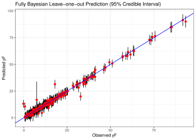
Figure 11: Fully Bayesian out-of-sample predicted $\mathbf{y}^{F}$ with 95% credible interval over observed honeycomb field data $\mathbf{y}^{F}$.

Consider deploying these equations in our out-of-sample setup, re-using the new OSSs trained for the pointwise comparisons. Following a similar LOO setup, we derive $(\mathbf{y}^{F}_{i}\mid\mathbf{y}^{M}_{-i},\mathbf{y}^{F}_{-i},\mathbf{y}^{M}_{i},\mbox{\boldmath$\Phi$},\mathbf{u}^{(t)})\sim\mathcal{N}_{i}(\mathbf{m}_{i},\mathbf{V}_{i})$ via Eqs. (20–21) integrating over $\mathbf{u}$ by aggregating over Monte Carlo samples for $\{\mathbf{u}^{(t)}\}_{t=1}^{T}$ shown in bottom-left panels of Figure 9. When aggregating covariances, covariances of sample means are incorporated respecting the law of total variance. Figure 11 shows this fully Bayesian predicted mean with 95% credible interval over each observed $\mathbf{y}^{F}$. In contrast to to the previous leave-one-out experiments described in Eq. 17, which involved 292 LOO discrepancy terms $\hat{b}^{(-i)}(\cdot)$ via residuals $\mathbf{y}^{F}_{(-i)}-\hat{\mathbf{y}}^{M}_{(-i)}$ and $\mathbf{X}^{F}_{(-i)}$, results in Figure 11 provide full out-of-sample posterior predictive uncertainty for both the simulation and the discrepancy correction.

6 Discussion

Motivated by a computer model calibration problem the design of a seal used in turbines, we developed a thrifty new method to address several challenging features. Those challenges include a high-dimensional input space, local instability in computer model simulations, nonstationary simulator dynamics, and modeling for large computer experiments. Taken alone, each of these challenges has solutions that are, at least in some cases, well established in the literature. Taken together, a more deliberate and custom development was warranted. To meet those challenges, we developed the method of on-site surrogates. The construction of OSSs is motivated by the unique structure of the posterior distribution under study in the canonical Kennedy and O’Hagan, calibration framework, where predictions are needed only at a limited number of field data sites, no matter how big the computer experiment is. This unique structure allowed us to map a single, potentially high-dimensional problem, into a multitude of low-dimensional ones where computation can be performed in parallel. Two OSS-based calibration settings were entertained, one based on simple bias-corrected maximization and the other akin to the original KOH framework. Both were shown to empirically outperform simpler, yet high-powered, alternatives.

Despite its many attractive features, there is clearly much potential to refine this approach, in particular the design and modeling behind the OSSs. While simple Latin hypercube samples and GPs with exponential kernels and nuggets work well, several simple extensions could be quite powerful. The need for such extensions, along at least one avenue, is perhaps revealed by the final row of Figure 4. Those plots show bifurcating ISOTSEAL runs due to numerical instabilities. Although inflated nuggets enable smoothing over those regimes, the result is uniformly high uncertainty for all inputs rather than just near the trouble spot. The reason is that the GP formulation being used is still (locally) stationary. Specifically, the error structure is homoskedastic. Using a heteroskedastic GP instead (Binois et al.,, 2018), say via hetGP on CRAN (Binois and Gramacy,, 2018), could offer a potential remedy. In a follow-in paper Binois et al., (2019) showed how designs for effective hetGP modeling could be built up sequentially, balancing an appropriate amount of exploration and replication in order to effectively learn signal-to-noise relationships in the data. Such an approach could represent an attractive alternative to simple LHSs in $\mathbf{u}$-space.

Here we only entertained a single output $k_{\mathrm{dir}}$, at a single frequency, among a multitude of others and at other frequencies. In future work we plan to investigate a multiple output approach to calibration. Much work remains to assess the potential for such an approach, say via simple co-kriging (Ver Hoef and Barry,, 1998) or a linear model of co-regionalization (e.g., Wackernagel,, 1998). Our BHGE collaborators’ pilot study also indicated that there could potentially be input-dependent variations in the best setting of the friction factors. That is, we could be looking at a $\hat{\mathbf{u}}(\mathbf{x})$, perhaps for a subset of the coordinates of the 13-dimensional $\mathbf{x}$ input. Whether a simple partition-based or linear scheme might be appropriate, or if something more nonparametric like (Brown and Atamturktur,, 2018) is required, remains an open question.

We’d like to close with a thought on confounding and identifiability, an ever-present concern in the KOH setting. OSSs are no help here, essentially chopping up the design space, limiting information sharing and reducing the (Bayesian) learning that could transpire about calibration parameters compared to the usual (global) setup. Although we have seen no evidence of concern, it is possible that OSSs would exacerbate the problem. However, we note that the underlying framework – linking a latent $\mathbf{u}$-variable to a nonparametric discrepancy – is identical whether or not OSSs are deployed. Accordingly, simplifications (Tuo and Wu,, 2015) or extensions (Plumlee,, 2017) are similarly viable as a means of limiting sources of confounding that challenges identifiability.

There are many reasons to calibrate, with KOH or otherwise. One is simply predictive; another is to get a sense of how the apparatus could be tuned, or to quantify how much information is in the data (and prior) about promising $\mathbf{u}$ settings. Both are very doable, and worth doing, even in the face of confounding. Our posterior summaries for $\mathbf{u}$ are a testament in this regard. In our toy example, which has many features in common with the motivating honeycomb seal, the posterior is quite peaked. Does this mean our $\hat{\mathbf{u}}$ or Bayesian samples $\mathbf{u}^{(t)}$ have identified the right $\mathbf{u}^{*}$? Possibly not in general, except that we know the truth in this case and identification can be confirmed. Our posterior for $\mathbf{u}$ in the honeycomb example shows sharp concentration for some inputs, less for others, and interpretable correlation in one pair $(u_{3},u_{4})$. Our colleagues at BHGE were not surprised by these results, and found them to be helpful in designing new field experiments. Although we cannot be confident about identification in this example, KOH has been a useful exercise.

Acknowledgments

Authors JH, RBG, and MB are grateful for support from National Science Foundation grants DMS-1521702 and DMS-1821258. JH and RBG also gratefully acknowledge funding from a DOE LAB 17-1697 via subaward from Argonne National Laboratory for SciDAC/DOE Office of Science ASCR and High Energy Physics. The work of MB is partially supported by the U.S. Department of Energy, Office of Science, Office of Advanced Scientific Computing Research, under Contract No. DE-AC02-06CH11357. We thank Andrea Panizza for early NLS work on this project, and for initiating the line of research. We are grateful to two referees for thoughtful suggestions which led to many improvements. Finally, we wish to thank our collaborators at Baker Hughes/GE for being generous with their data, their time, and their expertise.

7 Appendix: Calibration under uniform prior

For completeness, we provide calibration results under a uniform prior in Figure 12, complementing those from Figure 9 under $\mathrm{Beta}(2,2)$.

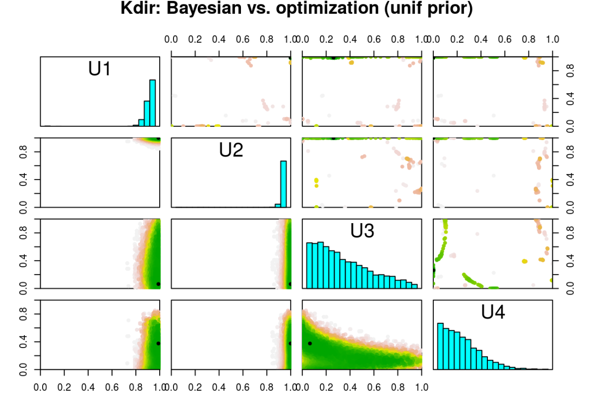
Figure 12: Bayesian KOH (lower and diagonal) posterior for $\mathbf{u}$ vs. modularized optimization (upper) analog, both under an independent uniform prior for $\mathbf{u}$. Colors are derived from ranks of posterior probabilities to aid in visualization. Modularized results are from 500 converged optimization under random initialization. Black dots indicate MAP values.

Compared with those results, the ones shown here more heavily concentrate on the boundaries of the study region. Also, somewhat more inconsistency exists between the modular/opt results and the fully Bayesian analog. The regularization effect of the $\mathrm{Beta}(2,2)$ leads to better numerics.

References

- Abramson et al., (2013) Abramson, M., Audet, C., Couture, G., Dennis, Jr., J., Le Digabel, S., and Tribes, C. (2013). “The NOMAD project.” Software available at http://www.gerad.ca/nomad.
- Ba and Joseph, (2012) Ba, S. and Joseph, V. (2012). “Composite Gaussian process models for emulating expensive functions.” Annals of Applied Statistics, 6, 4, 1838–1860.
- Bastos and O’Hagan, (2009) Bastos, L. and O’Hagan, A. (2009). “Diagnostics for Gaussian Process Emulators.” Technometrics, 51, 4, 425–438.
- Binois and Gramacy, (2018) Binois, M. and Gramacy, R. B. (2018). hetGP: Heteroskedastic Gaussian Process Modeling and Design under Replication. R package version 1.0.3.
- Binois et al., (2018) Binois, M., Gramacy, R. B., and Ludkovski, M. (2018). “Practical heteroskedastic Gaussian process modeling for large simulation experiments.” Journal of Computational and Graphical Statistics, 27, 4, 808–821.
- Binois et al., (2019) Binois, M., Huang, J., Gramacy, R. B., and Ludkovski, M. (2019). “Replication or exploration? Sequential design for stochastic simulation experiments.” Technometrics, 61, 1, 7–23.
- Bornn et al., (2012) Bornn, L., Shaddick, G., and Zidek, J. (2012). “Modelling Nonstationary Processes Through Dimension Expansion.” J. of the American Statistical Association, 107, 497, 281–289.
- Brown and Atamturktur, (2018) Brown, D. A. and Atamturktur, S. (2018). “Nonparametric Functional Calibration of Computer Models.” Statistica Sinica, 28, 721–742.
- Byrd et al., (1995) Byrd, R., Qiu, P., Nocedal, J., , and Zhu, C. (1995). “A Limited Memory Algorithm for Bound Constrained Optimization.” Journal on Scientific Computing, 16, 5, 1190–1208.
- Carnell, (2018) Carnell, R. (2018). lhs: Latin Hypercube Samples. R package version 0.16.
- D’Souza and Childs, (2002) D’Souza, R. J. and Childs, D. W. (2002). “A Comparison of Rotordynamic-Coefficient Predictions for Annular Honeycomb Gas Seals Using Three Different Friction-Factor Models.” Journal of Tribology, 124, 3, 524–529.
- Gelfand and Smith, (1990) Gelfand, A. E. and Smith, A. F. M. (1990). “Sampling-Based Approaches to Calculating Marginal Densities.” Journal of the American Statistical Association, 85, 410, 398–409.
- Gramacy, (2016) Gramacy, R. (2016). “laGP: Large-Scale Spatial Modeling via Local Approximate Gaussian Processes in R.” Journal of Statistical Software, Articles, 72, 1, 1–46.
- Gramacy and Lee, (2012) Gramacy, R. and Lee, H. (2012). “Cases for the nugget in modeling computer experiments.” Statistics and Computing, 22, 3, 713–722.
- Gramacy and Apley, (2015) Gramacy, R. B. and Apley, D. W. (2015). “Local Gaussian process approximation for large computer experiments.” Journal of Computational and Graphical Statistics, 24, 2, 561–578.
- Gramacy et al., (2015) Gramacy, R. B., Bingham, D., Holloway, J. P., Grosskopf, M. J., Kuranz, C. C., Rutter, E., Trantham, M., and Drake, R. P. (2015). “Calibrating a large computer experiment simulating radiative shock hydrodynamics.” Annals of Applied Statistics, 9, 3, 1141–1168.
- Gramacy and Sun, (2018) Gramacy, R. B. and Sun, F. (2018). laGP: Local approximate Gaussian process regression. R package version 1.5-2.
- Gul et al., (2018) Gul, E., Joseph, V. R., Yan, H., and Melkote, S. N. (2018). “Uncertainty quantification of machining simulations using an in situ emulator.” Journal of Quality Technology, 50, 3, 253–261.
- Hastings, (1970) Hastings, W. K. (1970). “Monte Carlo Sampling Methods Using Markov Chains and Their Applications.” Biometrika, 57, 1, 97–109.
- Higdon et al., (2004) Higdon, D., Kennedy, M., Cavendish, J. C., Cafeo, J. A., and Ryne, R. D. (2004). “Combining field data and computer simulations for calibration and prediction.” SIAM Journal on Scientific Computing, 26, 2, 448–466.
- Hirs, (1973) Hirs, G. G. (1973). “A Bulk-Flow Theory for Turbulence in Lubricant Films.” Journal of Lubrication Technology, 95, 2, 137–145.
- Hoff, (2009) Hoff, P. D. (2009). A first course in Bayesian statistical methods. Springer Science & Business Media.
- Kass et al., (1998) Kass, R. E., Carlin, B. P., Gelman, A., and Neal, R. M. (1998). “Markov Chain Monte Carlo in Practice: A Roundtable Discussion.” The American Statistician, 52, 2, 93–100.
- Kennedy and O’Hagan, (2001) Kennedy, M. C. and O’Hagan, A. (2001). “Bayesian calibration of computer models.” Journal of the Royal Statistical Society, Series B, 63, 3, 425–464.
- Kleynhans and Childs, (1997) Kleynhans, G. and Childs, D. (1997). “The Acoustic Influence of Cell Depth on the Rotordynamic Characteristics of Smooth-Rotor/Honeycomb-Stator Annular Gas Seals.” ASME Journal of Engineering for Gas Turbines and Power, 949–957.
- Le Digabel, (2011) Le Digabel, S. (2011). “Algorithm 909: NOMAD: Nonlinear Optimization with the MADS algorithm.” ACM Transactions on Mathematical Software, 37, 4, 44:1–44:15.
- Liu et al., (2009) Liu, F., Bayarri, M., and Berger, J. (2009). “Modularization in Bayesian analysis, with emphasis on analysis of computer models.” Bayesian Analysis, 4, 1, 119–150.
- Morris and Mitchell, (1995) Morris, M. D. and Mitchell, T. J. (1995). “Exploratory designs for computational experiments.” Journal of Statistical Planning and Inference, 43, 381–402.
- Nash, (2016) Nash, J. C. (2016). nlmrt: Functions for Nonlinear Least Squares Solutions. R package version 2016.3.2.
- Petersen et al., (2008) Petersen, K. B., Pedersen, M. S., et al. (2008). “The matrix cookbook.” Technical University of Denmark, 7, 15.
- Plumlee, (2017) Plumlee, M. (2017). “Bayesian calibration of inexact computer models.” Journal of the American Statistical Association, 112, 519, 1274–1285.
- R Core Team, (2018) R Core Team (2018). optim: General-purpose Optimization. R package version 3.6.0.
- Rasmussen and Williams, (2006) Rasmussen, C. E. and Williams, C. (2006). Gaussian Processes for Machine Learning. MIT Press.
- Sacks et al., (1989) Sacks, J., Welch, W. J., Mitchell, T. J., and Wynn, H. P. (1989). “Design and analysis of computer experiments.” Statistical science, 4, 409–423.
- Santner et al., (2003) Santner, T. J., Williams, B. J., and Notz, W. I. (2003). The design and analysis of computer experiments. Springer Science & Business Media.
- Tuo and Wu, (2015) Tuo, R. and Wu, C. F. J. (2015). “Efficient calibration for imperfect computer models.” Ann. Statist., 43, 6, 2331–2352.
- Vannarsdall, (2011) Vannarsdall, M. L. (2011). “Measured Results for a New Hole-Pattern Annular Gas Seal Incorporating Larger Diameter Holes, Comparisons to Results for a Traditional Hole-Pattern Seal and Predictions.” Available electronically from http://hdl.handle.net/1969.1/ETD-TAMU-2011-08-9759.
- Ver Hoef and Barry, (1998) Ver Hoef, J. and Barry, R. P. (1998). “Constructing and Fitting Models for Cokriging and Multivariate Spatial Prediction.” Journal of Statistical Planning and Inference, 69, 275–294.
- Wackernagel, (1998) Wackernagel, H. (1998). Multivariate Geostatistics. New York: Springer.
- Ypma et al., (2017) Ypma, J., Borchers, H. W., and Eddelbuettel, D. (2017). nloptr: R interface to NLopt. R package version 1.0.4.