480pt 665pt 5pt 5pt -10pt

The experimental sensitivity to $\mu\to e$ conversion on nuclei is set to improve by four orders of magnitude in coming years. However, various operator coefficients add coherently in the amplitude for $\mu\!\to\!e~{}{\rm conversion}$, weighted by nucleus-dependent functions, and therefore in the event of a detection, identifying the relevant new physics scenarios could be difficult. Using a representation of the nuclear targets as vectors in coefficient space, whose components are the weighting functions, we quantify the expectation that different nuclear targets could give different constraints. We show that all but two combinations of the 10 Spin-Independent (SI) coefficients could be constrained by future measurements, but discriminating among the axial, tensor and pseudoscalar operators that contribute to the Spin-Dependent (SD) process would require dedicated nuclear calculations. We anticipate that $\mu\!\to\!e~{}{\rm conversion}$ could constrain 10 to 14 combinations of coefficients; if $\mu\to e\gamma$ and $\mu\to e\bar{e}e$ constrain eight more, that leaves 60 to 64 “flat directions” in the basis of QED$\times$QCD-invariant operators which describe $\mu\to e$ flavour change below $m_{W}$.

1 Introduction

The observation of neutrino mixing and masses implies that flavour cannot be conserved among charged leptons. However, despite a long programme of experimental searches for various processes, charged lepton flavour violation (CLFV) at a point has yet to be observed.

For $\mu\leftrightarrow e$ flavour change, the current most stringent bound is $BR(\mu\to e\gamma)\leq 4.2\times 10^{-13}$ from the MEG collaboration [1] at PSI. This sensitivity will improve by one order of magnitude in coming years [2], and the Mu3e experiment [3] at PSI aims to reach $BR(\mu\to e\bar{e}e)\sim 10^{-16}$. Several experiments under construction will improve the sensitivity to $\mu\!\to\!e~{}{\rm conversion}$ on nuclei: The COMET [4] at J-PARC and the Mu2e [5] at FNAL plan to reach branching ratios of $BR(\mu Al\to eAl)\sim 10^{-16}$. The PRISM/PRIME proposal [6] aims to probe $\sim 10^{-18}$, and at the same time enables to use heavy $\mu\!\to\!e~{}{\rm conversion}$ targets with shorter lifetimes of their muonic atoms, thanks to its designed pure muon beam with no pion contamination. This enhanced sensitivity and broader selection of $\mu\!\to\!e~{}{\rm conversion}$ targets motivate our interest in low-energy $\mu\leftrightarrow e$ flavour change.

In the coming years, irrespective of whether CLFV is observed or further constrained, it is important to maximise the amount of information that experiments can obtain about the New Physics responsible for CLFV. This is especially challenging for the operators involving nucleons or quarks, because in $\mu\to e$ conversion, the contributing coefficients add in the amplitude. So in this paper, we consider $\mu\to e$ conversion on nuclei, and present a recipe for selecting targets such that they constrain or measure different CLFV parameters. Reference [10] is an earlier discussion of the prospects of distinguishing models with $\mu\!\to\!e~{}{\rm conversion}$. A more recent publication [11] about Spin-Dependent $\mu\to e$ conversion studied what could be learned about models or operator coefficients, from targets with and without spin. In this letter, we follow the perspective of [11], focussing on the Spin Independent process, and explore how many independent constraints can be obtained on operator coefficients.

We assume that the New Physics responsible for $\mu\to e$ conversion is heavy, and parametrise it in Effective Field Theory (EFT) [12, 13, 14, 15]. Section 2 gives the $\mu\!\to\!e~{}{\rm conversion}$ rate, and the effective Lagrangian at the experimental scale ($\sim$ GeV), in terms of operators that are QED invariant, labelled by their Lorentz structure, and constructed out of electrons, muons and nucleons ($p$ and $n$). In Section 3 we divide the rate into pieces that do not interfere with each other. Section 4 is a toy model of two observables that depend on a sum of theoretical parameters, which illustrates the impact of theoretical uncertainties on the determination of operator coefficients. It is well-known, since the study of Kitano, Koike and Okada (KKO) [16], that different target nuclei have different relative sensitivity to the various operator coefficients. In Section 5, using the notion of targets as vectors in the space of operator coefficients introduced in Reference [11], we explore which current experimental bounds can give independent constraints on operator coefficients, given the current theoretical uncertainties. Section 6 discusses the prospects of future experiments, Section 7 compares the number of operator coefficients to the number of constraints that could be obtained from $\mu\!\to\!e~{}{\rm conversion}$, $\mu\to e\bar{e}e$ and $\mu\to e\gamma$, and Section 8 is the summary.

2 $\bm{\mu\!\to\!e~{}{\rm conversion}}$

$\mu\!\to\!e~{}{\rm conversion}$ is the process where an incident $\mu^{-}$ is captured by a nucleus, and tumbles down to the $1s$ state. The muon can then interact with the nucleus, by exchanging a photon or via a contact interaction, and turn into an electron which escapes with an energy $\sim m_{\mu}$. This process has been searched for in the past with various target materials, as summarised in table 1; the best existing bound is $BR(\mu Au\to eAu)<7\times 10^{-13}$ on Gold ($Z=79$) from SINDRUM-II [17].

The interaction of the muon with the nucleus can be parametrised at the experimental scale ($\Lambda_{expt}$) in Effective Field Theory, via dipole operators and a variety of 2-nucleon operators :

$${\cal L}_{\mu A\rightarrow eA}(\Lambda_{expt}) = -\frac{4G_{F}}{\sqrt{2}}\sum_{N=p,n}{\Big{[}}m_{\mu}\left(C_{DL}\overline{e_{R}}\sigma^{\alpha\beta}\mu_{L}F_{\alpha\beta}+C_{DR}\overline{e_{L}}\sigma^{\alpha\beta}\mu_{R}F_{\alpha\beta}\right)$$ (1)

$$+\left(\widetilde{C}^{(NN)}_{SL}\overline{e}P_{L}\mu+\widetilde{C}^{(NN)}_{SR}\overline{e}P_{R}\mu\right)\overline{N}N$$

$$+\left(\widetilde{C}^{(NN)}_{P,L}\overline{e}P_{L}\mu+\widetilde{C}^{(NN)}_{P,R}\overline{e}P_{R}\mu\right)\overline{N}\gamma_{5}N$$

$$+\left(\widetilde{C}^{(NN)}_{VL}\overline{e}\gamma^{\alpha}P_{L}\mu+\widetilde{C}^{(NN)}_{VR}\overline{e}\gamma^{\alpha}P_{R}\mu\right)\overline{N}\gamma_{\alpha}N$$

$$+\left(\widetilde{C}^{(NN)}_{A,L}\overline{e}\gamma^{\alpha}P_{L}\mu+\widetilde{C}^{(NN)}_{A,R}\overline{e}\gamma^{\alpha}P_{R}\mu\right)\overline{N}\gamma_{\alpha}\gamma_{5}N$$

$$+\left(\widetilde{C}^{(NN)}_{Der,L}\overline{e}\gamma^{\alpha}P_{L}\mu+\widetilde{C}^{(NN)}_{Der,R}\overline{e}\gamma^{\alpha}P_{R}\mu\right)i(\overline{N}\stackrel{{\scriptstyle\leftrightarrow}}{{\partial_{\alpha}}}\gamma_{5}N)$$

$$+\left(\widetilde{C}^{(NN)}_{T,L}\overline{e}\sigma^{\alpha\beta}P_{L}\mu+\widetilde{C}^{(NN)}_{T,R}\overline{e}\sigma^{\alpha\beta}P_{R}\mu\right)\overline{N}\sigma_{\alpha\beta}N+h.c.{\Big{]}}~{}~{}~{}.$$

Since the electron is relativistic, and the nucleons not, it is convenient to use a chiral basis for the lepton current, but not for the nucleons.

This basis of nucleon operators is chosen because it represents the minimal set onto which two-lepton-two-quark, and two-lepton-two-gluon operators can be matched at the leading order in $\chi$PT . This explains the presence of the derivative operators $\widetilde{{\cal O}}^{(NN)}_{Der,X}$, which represent pion exchange between the leptons and nucleons at finite momentum transfer. They give a contribution to Spin-Dependent $\mu\to e$ conversion that is comparable to the $\widetilde{{\cal O}}^{(NN)}_{A,X}$ operators [11]. We do not count the coefficients of the derivative operators as independent parameters, because their effects could be included as a momentum-transfer-dependence of the $G_{A}^{N,q}$ factors that relate quark to nucleon axial operators [11].

Like in WIMP scattering on nuclei, the muon can interact coherently with the charge or mass distribution of the nucleus, called the “Spin Independent” (SI) process, or it can have “Spin-Dependent” (SD) interactions[19] with the nucleus at a rate that does not benefit from the atomic-number-squared enhancement of the SI rate. The Dipole, Scalar and Vector operators will contribute to the SI rate (with a small admixture of the Tensor, see eqn 3), and the Axial, Tensor and Pseudoscalar operators contribute to the SD rate.

The SI contribution to the branching ratio for $\mu\!\to\!e~{}{\rm conversion}$ on the nucleus $A$ (${BR}_{SI}(A\mu\to Ae)$), was calculated by Kitano, Koike and Okada (KKO) [16] to be

$${\rm BR}_{SI}(\mu A\to eA) = \frac{32G_{F}^{2}m_{\mu}^{5}}{\Gamma_{cap}}{\Big{[}}\big{|}\widetilde{C}^{pp}_{V,R}V^{(p)}+\widetilde{C}^{pp^{\prime}}_{S,L}S^{(p)}+\widetilde{C}^{nn}_{V,R}V^{(n)}+\widetilde{C}^{nn^{\prime}}_{S,L}S^{(n)}+C_{D,L}\frac{D}{4}\big{|}^{2}+\{L\leftrightarrow R\}~{}{\Big{]}}~{}~{},$$ (2)

where $\Gamma_{capt}$ is the rate for the muon to transform to a neutrino by capture on the nucleus [16, 20], ($=0.7054\times 10^{6}$/sec in Aluminium). The nucleus ($A$) and nucleon($N\in\{n,p\}$)-dependent “overlap integrals” $D_{A}$, $S_{A}^{(p)}$, $V_{A}^{(p)}$, $S_{A}^{(n)}$, $V_{A}^{(n)}$, correspond to the integral over the nucleus of the lepton wavefunctions and the appropriate nucleon density. These overlap integrals will play a central role in our analysis, and are given in KKO [16]. The primed scalar coefficient includes a small part of the tensor coefficient, because the tensor contributes at finite momentum transfer to the SI process [19, 11]:

$$\widetilde{C}_{{S},X}^{NN^{\prime}}=\widetilde{C}_{{S},X}^{NN}+\frac{2m_{\mu}}{m_{N}}\widetilde{C}_{T,X}^{NN}~{}~{}~{}.~{}~{}~{}$$ (3)

The SD rate depends on the distribution of spin in the nucleus, and therefore requires detailed nuclear modelling. The tensor and axial vector contributions were estimated in References [19, 11] for light ($Z\mathrel{\vbox{\hbox{$<$}\nointerlineskip\hbox{$\sim$}}}20$) nuclei, where the muon wavefunction is wider than the radius of the nucleus, and the electron can be approximated as a plane wave. In this limit, where the muon wavefunction can be factored out of the nuclear spin-expectation-value, the nuclear calculation of SD WIMP scattering on the quark axial current can be used for $\mu\!\to\!e~{}{\rm conversion}$. The SD branching ratio on a target $A$ of charge $Z$, with a fraction $\epsilon_{I}$ of isotope $I$ with spin $J_{I}$, can be estimated as

$${\rm BR}_{SD}(\mu A\to eA)\!\! = \!\!\frac{8G_{F}^{2}m_{\mu}^{5}(\alpha Z)^{3}}{\Gamma_{cap}\pi^{2}}\left[\sum_{I}4\epsilon_{I}\frac{J_{I}+1}{J_{I}}\,\Big{|}S^{I}_{p}(\widetilde{C}_{{A},L}^{pp}+2\widetilde{C}_{T,R}^{pp})+S^{I}_{n}(\widetilde{C}_{{A},L}^{nn}+2\widetilde{C}_{T,R}^{nn})\Big{|}^{2}\ \frac{S_{I}(m_{\mu})}{S_{I}(0)}+\{L\leftrightarrow R\}\right]$$

where $S_{p}^{I}$ is the proton spin expectation value in isotope $I$ at zero momentum transfer, and ${S_{I}(m_{\mu})}/{S_{I}(0)}$ is a finite momentum transfer correction, which has been calculated for the axial current in some nuclei(see eg References [21, 22] for Aluminium; this factor includes the derivative operators $\widetilde{{\cal O}}^{(NN)}_{Der,X}$). The targets which have been used for $\mu\!\to\!e~{}{\rm conversion}$ searches are listed in Table 1, with the abundances of some spin-carrying isotopes, and some results for the proton and neutron spin expectation values.

target	isotopes[abundance]	J	$S_{p}^{A}$ , $S_{n}^{A}$	$S_{I}(m_{\mu})/S_{I}(0)$	$B_{Z}$	BR(90% C.L.)
Sulfur	Z=16,A= 32[95%]	0				$<7\times 10^{-11}$ [23]
Titanium	Z=22,A= 48[74%]	0			234	$<4.3\times 10^{-12}$[17]
	Z=22,A= 47[7.5%]	5/2	0.0 , 0.21[24]	$\sim$0.12
	Z=22,A= 49[5.4%]	7/2	0.0 , 0.29[24]	$\sim$0.12
Copper	Z=29,A= 63[70%]	3/2				$BR\leq 1.6\times 10^{-8}$[25]
	Z=29,A= 65[31%]	3/2
Gold	Z =79,A =197[100%]	5/2	-(0.52$\to$0.30), 0.0		285	$BR<7\times 10^{-13}$[17]
Lead	Z=82, A=206[24%]	0				$BR<4.6\times 10^{-11}$ [17]
	Z=82, A=207[22%]	1/2	0.0 ,-0.15 [24]	0.55[28], $\sim$.026
	Z=82, A=208[52%]	0
Aluminium	Z=13,A= 27[100%]	5/2	0.34, 0.030 [21, 22]	0.29 [21, 22]	132	$\to 10^{-16}$

Table 1: Current experimental bounds on $\mu\!\to\!e~{}{\rm conversion}$ (the last line gives the future sensitivity on Aluminium), and parameters relevant to the SD calculation. The isotope abundances are from [30]. The parameter $B_{Z}$ is defined in eqn (8). The estimate for $S_{p}^{Au}$ is based on the Odd Group Model of [24], assuming J=1/2. The estimated form factors $S_{I}(m_{\mu})/S_{I}(0)$ for Titanium and Lead are an extrapolation from [11], discussed in the Appendix.

3 To determine or constrain how many coefficients?

The Lagrangian of eqn (1) contains twenty-two unknown operator coefficients (not counting the derivative operators as discussed after eqn (1)). These coefficients contribute to various observables, so can be constrained, or measured, in different ways:

1. we neglect the two dipole coefficients, because the upcoming MEG II and Mu3e experiments, respectively searching for $\mu\to e\gamma$ and $\mu\to e\bar{e}e$, have a slightly better sensitivity: if MEG II and Mu3e set bounds $BR(\mu\to e\gamma)<6\times 10^{-14}$ and $BR(\mu\to e\bar{e}e)<10^{-16}$, this would translate to $|C_{D,X}|\leq 2.0\times 10^{-9}$ (see eqn 20). Whereas a SI $\mu\!\to\!e~{}{\rm conversion}$ branching ratio of $10^{-16}$ on Aluminium can be sensitive to $|C_{D,X}|\mathrel{\vbox{\hbox{$>$}\nointerlineskip\hbox{$\sim$}}}3.1\times 10^{-9}$.

2. the remaining 20 coefficients involving nucleons can be divided into two classes, labelled by the chirality/helicity of the outgoing (relativistic) electron. The interference between these classes is usually neglected (suppressed by $m^{2}_{e}/m^{2}_{\mu}$), so an experimental upper bound on the rate simultaneously sets bounds on the coefficients of both chiralities. If a $\mu\!\to\!e~{}{\rm conversion}$ signal is observed with polarised muonic atoms, it could be possible to identify the chirality of the operator by measuring an angular distribution of the electron with respect to the muon spin direction . For simplicity, we will in the following only discuss the ten operators that create an $e_{L}$.

   Notice that the conventions of eqn (1) label operator coefficients with the chirality of the muon, which is opposite to the electron for dipole, scalar, pseudoscalar and tensor operators.

3. Finally, the operators can also be divided into those that mediate SI or SD conversion. In the body of the paper, we will discuss the SI rate, to which contribute the dipole that we neglect, and the vector and scalar on the neutron and proton. These appear in the amplitude weighted by overlap integrals (see after eqn 2), which are nucleus-dependent. This suggests that to constrain the four operator coefficients, one just needs to search for $\mu\!\to\!e~{}{\rm conversion}$ on four sufficiently different targets. (In order to measure the SI coefficients independently from SD ones, the targets could/should be chosen without SD contributions.)

   In the Appendix A, we make some remarks on the SD rate, which can be sensitive to six coefficients. However, quantitative calculations would require nuclear matrix elements that we did not find in the literature.

4 Targets as vectors, and the problem of theoretical uncertainties

In a previous publication[11], a representation of targets as vectors in coefficient space was introduced. The targets are labelled by $Z$, and for SI transitions, the elements of the vector are the overlap integrals of KKO [16]:

$$\vec{v}_{Z}=\left(\frac{D_{Z}}{4},V^{(p)}_{Z},S^{(p)}_{Z},V^{(n)}_{Z},S^{(n)}_{Z}\right)$$ (5)

The aim was to give a geometric, intuitive measure of different targets ability to distinguish coefficients. If the operator coefficients are lined up in a pair of vectors labelled by the chirality of the outgoing electron, such that for $e_{L}$:

$$\vec{C}_{L}=(\widetilde{C}_{D,R},\widetilde{C}_{V,L}^{pp},\widetilde{C}_{S,R}^{pp},\widetilde{C}_{V,L}^{nn},\widetilde{C}_{S,R}^{nn})$$ (6)

(and similarly for $\vec{C}_{R}$), then the SI Branching Ratio on target $Z$ (see eqn (2) can be written

$$BR_{SI}=B_{Z}{\Big{[}}|\hat{v}_{Z}\cdot\vec{C}_{L}|^{2}+|\hat{v}_{Z}\cdot\vec{C}_{R}|^{2}{\Big{]}}~{}~{}~{},$$ (7)

where the numerical value of the coefficient

$$B_{Z}=\frac{32G_{F}^{2}m_{\mu}^{5}|\vec{v}_{Z}|^{2}}{\Gamma_{cap}(Z)}$$ (8)

is listed in table 1 for some targets. If two target vectors are parallel, they probe the same combination of couplings, and if they are misaligned, they could allow to distinguish among the coefficients.

To quantify how “misaligned” targets need to be, in order to differentiate among coefficients, we should take into account the theoretical uncertainties. These are a significant complication, because they make uncertain which combination of coefficients is constrained by which target. To illustrate the problem, we suppose coefficient space is two-dimensional. This allows to draw pictures.

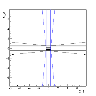
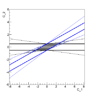
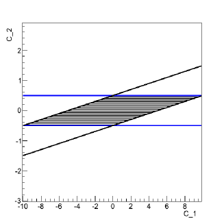
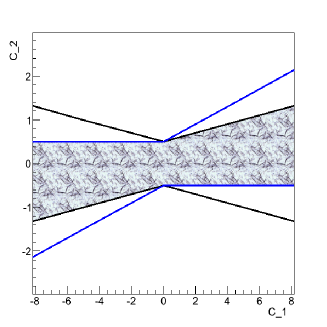
Figure 1: Illustration of the impact of theoretical uncertainties on the determination of operator coefficients, when combining results from two experiments. The allowed region neglecting theory uncertainties is stripped; the larger grey areas are allowed when theoretical uncertainties are included. The upper left plots is for two experiments that measure orthogonal parameters, the upper right plot is for two experiments who measure correlated parameters but with manageable uncertainty, and the lower two plots represent the case where the two experiments do not give independent information when the theory uncertainty is included.

If a first observable $T_{1}$, can be computed with negligible theoretical uncertainty to depend on $|C_{1}|^{2}$, and a second observable $T_{2}$, similarly can be computed to depend on $|C_{2}|^{2}$, then the values of the coefficients respectively allowed by null results in the two experiments are inside the thick lines of the top left plot in Figure 1. The central stripped (dark) region is allowed when the two experimental results are combined. In reality, the allowed region should be more the shape of a circle, since the experimental uncertainties are (in part) statistical. However, we neglect this detail because it is not the subject of our discussion.

Suppose now that there is some theoretical uncertainty $\epsilon$ in the calculations, such that $T_{1}$ depends on $|C_{1}(1\pm\epsilon)\pm\epsilon C_{2}|^{2}$, and $T_{2}$ depends on $|C_{2}(1\pm\epsilon)\pm\epsilon C_{1}|^{2}$. Then provided $\epsilon\ll 1$ ($\epsilon\simeq\pi/32\simeq.1$ in the Figure), the regions respectively allowed by the two experiments are the bowties within the thin lines of the upper left plot in Figure1. The region allowed by the combined experiments is essentially unchanged (still the central square).

Consider next a situation more relevant to $\mu\!\to\!e~{}{\rm conversion}$, illustrated in the upper right plot of Figure 1. The second observable $T_{2}$ again depends on $|C_{2}(1\pm\epsilon)\pm\epsilon C_{1}|^{2}$, but $T_{1}$ depends on $|\cos\theta C_{2}-\sin\theta C_{1}|$, where $\theta\simeq\pi/8\pm\epsilon$. Neglecting theoretical uncertainties, the allowed regions for the two experiments are respectively between the thick blue lines, and thick black lines. The stripped diamond is the parameter range consistent with both experiments. But if the theory uncertainty is taken into account, the allowed regions of the two experiments are respectively enclosed by the thin blue and black lines. The region allowed by the combined observations is the grey diamond, which includes the stripped one. So we see that the theoretical uncertainty changes the allowed region by factors of ${\mathcal{O}}(1)$.

Finally, in the lower two plots of Figure 1, $T_{1}$ depends on $|\cos\theta C_{2}-\sin\theta C_{1}|$, where $\theta\simeq 2\epsilon\pm\epsilon$. If the theory uncertainty is neglected, as illustrated in the lower left plot, the region allowed by the two experiments corresponds to the stripped diamond. However, when the angle uncertainty is taken into account, both bars can be rotated towards each other, such that they point in the same direction, and any value of $C_{1}$ is allowed. This is illustrated in the lower right plot, where the allowed region is grey, and gives no constraint on $C_{1}$.

The allowed range for $C_{1}$ would be finite for

$$\theta>2\epsilon$$ (9)

which we take as the condition that two observables constrain independent directions in coefficient space. (Recall that $\theta$ is the angle between the two observables, represented as vectors in coefficient space, and $\epsilon$ is the theoretical uncertainty on the calculation of $\theta$).

For $\mu\!\to\!e~{}{\rm conversion}$, the theoretical uncertainties in the calculation of the rate and the overlap integrals were discussed in [11]. The current uncertainties were estimated as $\epsilon\mathrel{\vbox{\hbox{$<$}\nointerlineskip\hbox{$\sim$}}}10\,\%$. This is based on KKO’s estimate of the uncertainties in their overlap integrals, which is $\mathrel{\vbox{\hbox{$<$}\nointerlineskip\hbox{$\sim$}}}5\,\%$ for light nuclei, and $\mathrel{\vbox{\hbox{$<$}\nointerlineskip\hbox{$\sim$}}}10\,\%$ for heavier nuclei, and on NLO effects in $\chi$PT. These are parametrically $10\,\%$, and could, for instance change the form of eqn (7), as occurs in WIMP scattering [31], making it impossible to parametrise targets as vectors. In the following section, we take the current uncertainties to be $\epsilon\sim 10\,\%$, or possibly $5\,\%$ for light targets, implying that two targets can give independent constraints if they are misaligned by $\theta\mathrel{\vbox{\hbox{$>$}\nointerlineskip\hbox{$\sim$}}}.2$ (or possibly $\theta\mathrel{\vbox{\hbox{$>$}\nointerlineskip\hbox{$\sim$}}}.1$ for light targets).

5 Comparing current bounds

In section 3, it was suggested that the four scalar and vector coefficients could be constrained or measured by searching for $\mu\!\to\!e~{}{\rm conversion}$ in four “sufficiently different” targets. And we see from Table 1 that there is data for Sulfur, Titanium, Copper, Gold and Lead. However, as estimated in the previous section, “sufficiently different” means misaligned by 10-20%, so in this section, we calculate the misalignment between the targets for which there is data.

Recall that targets are described by vectors (see eqn 5), that live in the same space as the operator coefficients. However, the components of the target vectors are all positive, meaning the misalignment angle between any two target vectors is $<\pi/2$, or equivalently, that the target vectors point all in the first quadrant.

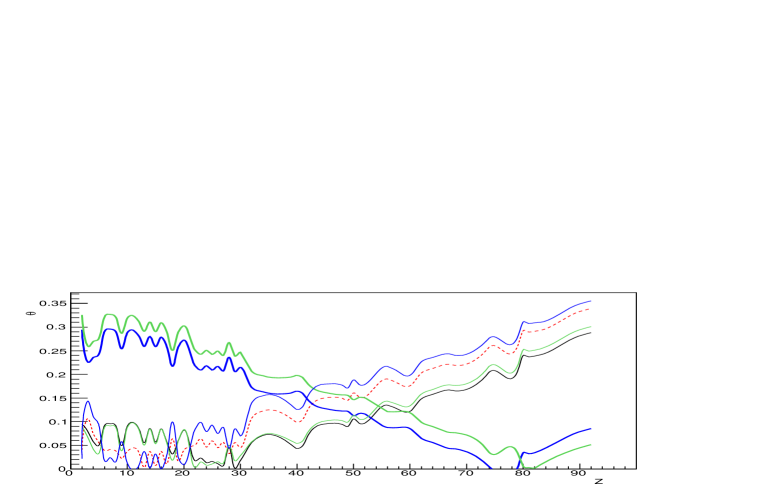
Figure 2: Angle $\theta$ between a target vector (eg dashed red = Aluminium) and other targets labelled by $Z$. The angle is obtained as in eqn (10), with all the dipole coefficients set to zero. The solid lines represent the targets for which there is currently data (see table 1). From smallest to largest value of $\theta$ at large $Z$, they are: thick green = Lead, thick blue = Gold, black = Copper, thin green = Titanium, dashed red = Aluminium, and thin blue is Sulfur. We assume that two targets can probe different coefficients if their misalignment angle is $\theta\mathrel{\vbox{\hbox{$>$}\nointerlineskip\hbox{$\sim$}}}0.2$ radians (or 0.1).

The angle between target $T$ and target $Z$ can be estimated from the normalised inner product

$$\frac{\vec{v}_{Z}\cdot\vec{v}_{T}}{|\vec{v}_{Z}||\vec{v}_{T}|}\simeq\cos\theta\simeq 1-\frac{\theta^{2}}{2}$$ (10)

In Figure 2 are plotted the misalignment angles between the targets of table 1, and the other possibilities given by KKO, labelled by $Z$. The thin blue line in Figure 2 (the line with largest $\theta$ at high $Z$) is the misalignment angle with respect to Sulfur, and the thin green line (the solid line with the second largest $\theta$ at high $Z$) is the misalignment angle with respect to Titanium. So the blue line at Z=22 (Titanium) is equal to the green line at 16 (Sulfur), and both give $\theta\sim 0.08$ between Sulfur and Titanium, suggesting that these constrain the same combination of coefficients. On the other hand, Gold probes different coefficients from the light targets (as anticipated by KKO [16]), but Gold and Lead cannot distinguish coefficients. Also Copper and Titanium do not give independent constraints. So the current experimental bounds on $\mu\!\to\!e~{}{\rm conversion}$ constrain two combinations of the four coefficients present in $\vec{C}_{L}$ (similarly, two combinations in $\vec{C}_{R}$). Thus, the current experimental bounds can be taken as the SINDRUM-II constraints from Titanium and Gold.

These two experimental bounds constrain coefficients in the two-dimensional space spanned by $\hat{v}_{Ti}$ and $\hat{v}_{Au}$. The bounds can be taken to apply to $\vec{C}\cdot\hat{v}_{Ti}$ and to $\vec{C}\cdot\hat{v}_{\perp}$, where $\vec{v}_{\perp}$ is component of the Gold target vector orthogonal to $\hat{v}_{Ti}$:

$$\hat{v}_{\perp}\equiv\frac{\hat{v}_{Au}-\cos\phi\hat{v}_{Ti}}{\sin\phi}$$ (11)

and $\phi$ is the angle between Gold and Titanium, so $\cos\phi=\hat{v}_{Ti}\cdot\hat{v}_{Au}$, and $\sin\phi=0.218$. The allowed values of the coefficients satisfy

$$BR_{Ti}\equiv BR(\mu Ti\to eTi) = 234|\vec{C}\cdot\hat{v}_{Ti}|^{2}<BR^{exp}_{Ti}\equiv 4.2\times 10^{-12}$$

$$BR_{Au}\equiv BR(\mu Au\to eAu) = 285|\cos\phi(\vec{C}\cdot\hat{v}_{Ti})+\sin\phi(\vec{C}\cdot\hat{v}_{\perp})|^{2}<BR^{exp}_{Au}\equiv 7.0\times 10^{-13}~{}~{}~{}.$$ (12)

We can construct a covariance matrix $V$, whose diagonal elements will be the constraints on $|\vec{C}\cdot\hat{v}_{Ti}|^{2}$ and $|\vec{C}\cdot\hat{v}_{\perp}|^{2}$, as

$$\vec{C}\cdot V^{-1}\cdot\vec{C}^{T}=\frac{BR_{Ti}}{BR_{Ti}^{exp}}+\frac{BR_{Au}}{BR_{Au}^{exp}}$$ (13)

which gives

$$|\vec{C}\cdot\hat{v}_{Ti}|^{2} \leq \frac{BR^{exp}_{Ti}}{B_{Ti}}=1.8\times 10^{-14}$$ (14)

$$|\vec{C}\cdot\hat{v}_{\perp}|^{2} \leq \frac{BR^{exp}_{Au}}{B_{Au}}\frac{1}{\sin^{2}\phi}+\frac{BR^{exp}_{Ti}}{B_{Ti}}\frac{\cos^{2}\phi}{\sin^{2}\phi}=0.44\times 10^{-12}$$ (15)

These bounds can be expressed in terms of quark operator coefficients at a higher scale by matching the nucleon operators onto quark operators, and running the coefficients up with Renormalisation Group Equations(RGEs). This matching and mixing process ensures that almost all $\mu\to e$ flavour-changing operators at the scale $m_{W}$ will contribute to $\mu\!\to\!e~{}{\rm conversion}$ at tree or one-loop order. We give an example in eqn (19).

6 Selecting future targets

The upcoming COMET and Mu2e experiments plan to use an Aluminium target, illustrated as a red dashed line in Figure 2. Unfortunately, it is only misaligned with respect to Titanium and Sulfur by a few percent, so with current theoretical uncertainties, Aluminium probes the same combination of SI coefficients as Titanium (and Sulfur).

It is therefore interesting to explore which targets could measure a different combinations of coefficients from Aluminium. As noted by KKO, the scalar and vector overlap integrals grow differently with $Z$, and using targets with different neutron to proton ratios could allow to differentiate coefficients on protons from those on neutrons. To quantify these differences, we introduce four orthonormal vectors in the space of nucleon overlap integrals:

$$\hat{e}_{1} = \frac{1}{2}(1,1,1,1)$$

$$\hat{e}_{2} = \frac{1}{2}(-1,-1,1,1)$$

$$\hat{e}_{3} = \frac{1}{2}(1,-1,1,-1)$$

$$\hat{e}_{4} = \frac{1}{2}(-1,1,1,-1)$$ (16)

Dotted into the coefficients, $\hat{e_{1}}$ measures the sum of coefficients, $\hat{e_{2}}$ is the difference between coefficients on protons and neutrons, $\hat{e_{3}}$ is the vector - scalar difference, and $\hat{e_{4}}$ is the remaining direction. All the targets are mostly aligned on $\hat{e}_{1}$; this is expected as the overlap integrals are of comparable size, and all positive . Indeed, for Aluminium, the target vector $\vec{v}_{Al}$ and $\hat{e}_{1}$ are almost parallel: $\vec{v}_{Al}\cdot\hat{e_{1}}\geq 0.997|\vec{v}_{Al}|$. So we suppose that this sum of coefficients is measured on Aluminium, and plot in Figure 3 the projection of the target vectors onto $\hat{e}_{2}$(thick, continuous line), $\hat{e}_{3}$ (dashed) and $\hat{e}_{4}$ (thin).

Figure 3: Projections of normalised target vectors $\hat{v}_{Z}=\vec{v}_{Z}/|\vec{v}_{Z}|$ onto the unit vectors of eqn 16. The jagged thick line is the projection onto $\hat{e}_{2}$ and parametrises the targets sensitivity to the $n$ to $p$ difference, the dotted black line is the projection onto $\hat{e}_{3}$ which parametrises the sensitivity to the scalar-vector difference, and the thin line is the projection onto the remaining direction.

Figure 3 shows that comparing heavy to light targets can distinguish scalar vs vector coefficients (or constrain both in the absence of a signal). The neutron to proton ratio also increases with atomic number, but perhaps a more promising target for making this difference would be Lithium, with four neutrons and three protons: the theoretical uncertainties could be more manageable, and the scalar-vector difference is suppressed. In addition, being light, it has a long lifetime, making it appropriate for the COMET and Mu2e experiments.

Unfortunately, it seems that $\mu\!\to\!e~{}{\rm conversion}$ targets have little sensitivity to $\hat{e}_{4}$, which measures some isospin-violating difference between scalars and vectors.

To illustrate the bounds that could be obtained in the future with COMET or Mu2e, we suppose that $\mu\!\to\!e~{}{\rm conversion}$ is not observed on Lithium($Z=3$) or Aluminium($Z=13$) at Branching Ratios $BR^{exp}_{Li},BR^{exp}_{Al}\ll BR^{exp}_{Au}$. We write the target vectors as

$$\hat{v}_{Al} \approx \hat{e}_{1}$$

$$\hat{v}_{Li} = (\hat{v}_{Li}\cdot\hat{e}_{1})\hat{e}_{1}+(\hat{v}_{Li}\cdot\hat{e}_{2})\hat{e}_{2}$$

$$\hat{v}_{Au} = (\hat{v}_{Au}\cdot\hat{e}_{1})\hat{e}_{1}+(\hat{v}_{Au}\cdot\hat{e}_{2})\hat{e}_{2}+(\hat{v}_{Au}\cdot\hat{e}_{3})\hat{e}_{3}~{}~{}~{}.$$

Then a $3\times 3$ covariance matrix can be obtained by combining the experimental upper bounds as in equation (13), which gives the constraints

$$|\vec{C}\cdot\hat{e}_{1}|^{2} \leq \frac{BR^{exp}_{Al}}{B_{Al}}$$ (17)

$$|\vec{C}\cdot\hat{e}_{2}|^{2} \leq \frac{BR^{exp}_{Li}}{B_{Li}}\frac{1}{|\hat{v}_{Li}\cdot\hat{e}_{2}|^{2}}+\frac{BR^{exp}_{Al}}{B_{Al}}\frac{|\hat{v}_{Li}\cdot\hat{e}_{1}|^{2}}{|\hat{v}_{Li}\cdot\hat{e}_{2}|^{2}}$$

$$|\vec{C}\cdot\hat{e}_{3}|^{2} \mathrel{\vbox{\hbox{$<$}\nointerlineskip\hbox{$\sim$}}} \frac{BR^{exp}_{Au}}{B_{Au}}\frac{1}{|\hat{v}_{Au}\cdot\hat{e}_{3}|^{2}}$$ (18)

where $|\hat{v}_{Li}\cdot\hat{e}_{2}|=0.142$, $|\hat{v}_{Au}\cdot\hat{e}_{3}|=0.217$, and terms were neglected in the bound on $|\vec{C}\cdot\hat{e}_{3}|$, assuming that $BR^{exp}_{Li},BR^{exp}_{Al}\ll BR^{exp}_{Au}$.

As mentioned at the end of the previous section, these bounds can be expressed in terms of coefficients of quark operators at some higher scale (for instance $m_{W}$ or the New Physics scale) by matching the nucleon coefficients to the quark coefficients at 2 GeV as $\widetilde{C}^{NN}_{O,X}=\sum_{q}G_{O}^{Nq}C_{O,X}^{qq}$ (where the $\{G_{O}^{Nq}\}$ are tabulated for instance in [11]), then expressing the coefficients at 2 GeV in terms of the high scale coefficients using the RGEs (see,eg [19, 11, 36]). The constraint of eqn (17) can be approximated as

$$\sqrt{\frac{BR^{exp}_{Al}}{33}} \mathrel{\vbox{\hbox{$>$}\nointerlineskip\hbox{$\sim$}}} {\Big{|}}3C^{uu}_{V,L}+3C^{dd}_{V,L}+11C^{uu}_{S,R}+11C^{dd}_{S,R}+0.84C^{ss}_{S,R}+\frac{4m_{N}}{27m_{c}}C^{cc}_{S,R}+\frac{4m_{N}}{27m_{b}}C^{bb}_{S,R}{\Big{|}}$$ (19)

$$\mathrel{\vbox{\hbox{$>$}\nointerlineskip\hbox{$\sim$}}} {\Big{|}}3C^{uu}_{V,L}+3C^{dd}_{V,L}+\frac{\alpha}{\pi}{\Big{[}}3C^{dd}_{A,L}-6C^{uu}_{A,L}{\Big{]}}\log+\frac{\alpha}{3\pi}[C^{ee}_{V,L}+C^{\mu\mu}_{V,L}]\log-\frac{\alpha}{3\pi}[C^{ee}_{A,L}+C^{\mu\mu}_{A,L}]\log$$

$$-\frac{2\alpha}{3\pi}{\Big{[}}2(C^{uu}_{V,L}+C^{cc}_{V,L})-(C^{dd}_{V,L}+C^{ss}_{V,L}+C^{bb}_{V,L})-(C^{ee}_{V,L}+C^{\mu\mu}_{V,L}+C^{\tau\tau}_{V,L}){\Big{]}}\log$$

$$+\lambda^{a_{S}}{\Big{(}}11C^{uu}_{S,R}+11C^{dd}_{S,R}+0.84C^{ss}_{S,R}+\frac{4m_{N}}{27m_{c}}C^{cc}_{S,R}+\frac{4m_{N}}{27m_{b}}C^{bb}_{S,R}{\Big{)}}$$

$$+\lambda^{a_{S}}\frac{\alpha}{\pi}{\Big{[}}\frac{13}{6}(11C^{uu}_{S,R}+\frac{4m_{N}}{27m_{c}}C^{cc}_{S,R})+\frac{5}{3}(11C^{dd}_{S,R}+0.84C^{ss}_{S,R}+\frac{4m_{N}}{27m_{b}}C^{bb}_{S,R}){\Big{]}}\log$$

$$-\lambda^{a_{T}}f_{TS}\frac{4\alpha}{\pi}{\Big{[}}22C^{uu}_{T,RR}+\frac{8m_{N}}{27m_{c}}C^{cc}_{T,RR}-11C^{dd}_{T,RR}-0.84C^{ss}_{T,RR}-\frac{4m_{N}}{27m_{b}}C^{bb}_{T,RR}){\Big{]}}\log{\Big{|}}$$

where in the first inequality, the quark coefficients are at the scale of 2 GeV, and we used the $\{G_{S}^{Nq}\}$ from the lattice [37]. In the second inequality, the coefficients are at $m_{W}$ (we suppress the dependence on scale to avoid cluttering the equations), $\log\equiv\log({m_{W}}/2{\rm GeV})\simeq 3.7$, $\lambda=\alpha_{s}(m_{W})/\alpha_{s}(2{\rm GeV})\simeq 0.44$, $f_{TS}=23(\lambda^{-16/23}-\lambda)/39/(1-\lambda)\simeq 1.45$, and $a_{S}=-12/23,a_{T}=4/23$. In both the first and second expressions, the tree-level tensor contribution to SI $\mu\!\to\!e~{}{\rm conversion}$ is neglected because it is smaller than the loop mixing into the scalar, and the scalar top coefficient $C_{S,R}^{tt}$ is also neglected.

7 Flat Directions and Tuning in EFTs

We now want to compare the number of constraints on $\mu\to e$ flavour-changing coefficients, to the number of operators in a “complete” basis — the difference will be the number of “flat” or unconstrained directions in parameter space.

In this counting, it is important to distinguish constraints from sensitivities. The bounds given in eqn (15) are constraints, meaning that the sum on the left cannot exceed the number on the right. This is different from the commonly-quoted sensitivities (or one-operator-at-a-time bounds), which give the value of a coefficient below which it is unobservable, and which do not allow for the possibility of cancellations among coefficients.

In the Effective Theory below $m_{W}$, a useful basis is the set of operators that are QED and QCD invariant, and that describe all the three or four-point functions that change lepton flavour from $\mu\to e$. These operators are of dimensions five, six and seven, and are listed, for instance, in [15]. We restrict to four-fermion operators whose second fermion bilinear is quark or lepton flavour-conserving (only these can contribute to $\mu\!\to\!e~{}{\rm conversion}$), in which case the basis contains 82 operators.

Eqn (15) gives the current $\mu\!\to\!e~{}{\rm conversion}$ bounds on four combinations of SI coefficients (two bounds for each electron chirality). There also should be two constraints on proton Spin-Dependent coefficients from Gold (since it has 79 protons), however the rate has not been calculated and could be quite small. In addition, there could be two constraints on neutron Spin-Dependent coefficients from Titanium, if the experimental target contained isotopes with an odd number of neutrons. So current data gives six or eight bounds.

With a wider variety of targets, and improved theoretical calculations, we showed in eqn (18) that it could be possible to constrain 6 of the 8 SI coefficients, and we argued that eight of the 12 SD coefficients could be constrained.

There are also stringent constraints on $\mu\to e$ flavour-changing operator coefficients from $\mu\to e\gamma$ and $\mu\to e\bar{e}e$. Constructing a covariance matrix for these two processes using the theoretical Branching Ratio formulae from [14] gives the bounds:

$$|C_{D,R}|^{2},|C_{D,L}|^{2} \leq \frac{BR^{exp}_{\mu\to e\gamma}BR^{exp}_{\mu\to e\bar{e}e}}{205e^{2}BR^{exp}_{\mu\to e\gamma}+384\pi^{2}BR^{exp}_{\mu\to e\bar{e}e}}$$

$$|C_{S,RR}|^{2},|C_{S,LL}|^{2} < 8BR^{exp}_{\mu\to e\bar{e}e}$$

$$|C_{V,RR}|^{2},|C_{V,LL}|^{2} \leq \frac{BR^{exp}_{\mu\to e\bar{e}e}}{2}\left(1+\frac{32e^{2}BR^{exp}_{\mu\to e\gamma}}{205e^{2}BR^{exp}_{\mu\to e\gamma}+384\pi^{2}BR^{exp}_{\mu\to e\bar{e}e}}\right)$$

$$|C_{V,RL}|^{2},|C_{V,LR}|^{2} \leq BR^{exp}_{\mu\to e\bar{e}e}\left(1+\frac{16e^{2}BR^{exp}_{\mu\to e\gamma}}{205e^{2}BR^{exp}_{\mu\to e\gamma}+384\pi^{2}BR^{exp}_{\mu\to e\bar{e}e}}\right)$$ (20)

where the four-lepton operators are ${\cal O}_{V,XY}=(\overline{e}\gamma^{\alpha}P_{X}\mu)(\overline{e}\gamma_{\alpha}P_{Y}e)$, ${\cal O}_{S,XY}=(\overline{e}P_{X}\mu)(\overline{e}P_{Y}e)$.

Combining the constraints from $\mu\to e\gamma$, $\mu\to e\bar{e}e$ and the current $\mu\!\to\!e~{}{\rm conversion}$ data, gives 14 to 16 constraints. In the future, $\mu\!\to\!e~{}{\rm conversion}$ could give two more SI constraints and four more SD bounds, for a total of 22. Each constraint applies to an lengthly linear combination of coefficients at $m_{W}$; nonetheless, there are therefore 60 to 68 combinations of coefficients (in the basis of QED$\times$QCD-invariant operators discussed above) which are unconstrained by $\mu\!\to\!e~{}{\rm conversion}$, $\mu\to e\gamma$ and $\mu\to e\bar{e}e$.

In order to constrain the multitude of flat directions, other processes can be considered, such as contact interaction searches at the LHC [38] or vector meson decays [39]. However, it might be difficult to find a sufficient number of restrictive constraints. Let us here speculate about how credible it is for a model to sit out along such a ”flat” direction, where the operator coefficients must be tuned against each other. We suppose that the coefficients parametrise the low energy behaviour of a renormalisable and natural high-scale model. However, since the coefficients are unknown functions of the model parameters, cancellations that reflect symmetries of the model could appear fortuitous in the EFT. We therefore allow arbitrary cancellations among coefficients at the high scale. Then we assume that the model cannot know the scale at which we do experiments (despite that this is determined by mass ratios which it does know), so we do not allow coefficients to cancel the logarithms from Renormalisation Group running.

We see from eqn (19) that the scalar and tensor operators run significantly with QCD, which suggests that they cannot cancel to more than one significant figure against each other or vector/axial coefficients. So a single constraint such as eqn (19), naturally implies three independent constraints on the vectors, scalars and tensors. Then within each subset of operators, the QED anomalous dimension matrix could be diagonalised, with, in general, non-degenerate anomalous dimensions. so coefficients that cancel at the high scale, may differ by ${\cal O}(\frac{\alpha}{4\pi}\log)$ at low energy. We therefore conclude that cancellations are only “natural” to 3 significant figures, among operator coefficients with unequal anomalous dimensions: if the constraint applies to a sum of operator coefficients $C_{j}$ weighted by numbers $n_{j}$

$$|\Sigma_{j}n_{j}C_{j}|<\epsilon$$ (21)

then each $C_{j}$ in the sum satisfies a “naturalness bound” of order

$$C_{j}\mathrel{\vbox{\hbox{$<$}\nointerlineskip\hbox{$\sim$}}}\frac{4\pi\epsilon}{\alpha n_{j}}~{}~{}~{}.$$ (22)

8 Summary

This letter studies the selection of targets for $\mu\!\to\!e~{}{\rm conversion}$, with the aim that they probe independent combinations of $\mu\to e$ flavour-changing parameters, while including the theoretical uncertainties of the calculation. The rate is parametrised via the operators given in eqn (1), and the theoretical uncertainties are reviewed in section 4. We take the current uncertainties to be $\sim 10\%$, and anticipate that this could be reduced to 5% in the future.

Using a parametrisation of targets as vectors in the space of operator coefficients, we reproduce the observation of Kitano, Koike and Okada (KKO) [16], that comparing light to heavy targets allows to distinguish scalar from vector operator coefficients. We also observe that comparing light targets with very different neutron-to-proton ratios could allow to distinguish operators involving neutrons from those involving protons. A reduction in the theory uncertainty would help to make this distinction. Lithium is the most promising target in the list for which KKO computed overlap integrals, however other light isotopes with higher $n/p$ ratios, such as Beryllium10, could be interesting to consider.

The Spin-Dependent (SD) conversion rate is mentioned in the Appendix. We reiterate that the neutron vs proton operators can be distinguished by searching for SD conversion on nuclei with an odd neutron and with an odd proton. Comparing the SD rate on light vs heavy nuclei could allow to distinguish axial from tensor coefficients, but dedicated nuclear calculations would be required to confirm this.

We conclude that $\mu\!\to\!e~{}{\rm conversion}$ currently can constrain six to eight independent combinations of operator coefficients, and in the future could constrain fourteen coefficients. Combined with the eight bounds that can be obtained from $\mu\to e\gamma$ and $\mu\to e\bar{e}e$, this gives 14 (now) to 22 (in the future) constraints on the 82 operators in a QED$\times$QCD invariant operator basis below $m_{W}$, so there remain 60-68 “flat directions”, or combinations of coefficients that are unconstrained by the data.

For a model to be situated along one of the many flat directions, requires cancellations among various operator coefficients. We argued that it would be “unnatural” to have cancellations between terms at different order in the $\alpha\log$ expansion of EFT, so coefficients can only cancel against each other up to ${\cal O}(\frac{\alpha}{4\pi}\log)$, and coefficients whose sum is constrained to be $\mathrel{\vbox{\hbox{$<$}\nointerlineskip\hbox{$\sim$}}}\epsilon$, should individually satisfy the “natural” bound $C\mathrel{\vbox{\hbox{$<$}\nointerlineskip\hbox{$\sim$}}}4\pi\epsilon/\alpha$.

Appendix A Appendix: the SD contribution

In this Appendix, we discuss how different targets could distinguish among the many operators that contribute to SD conversion.

We first recall the operators that contribute to the SD rate. For a fixed electron chirality, the pseudoscalar, axial vector and tensor nucleon currents become, in the non-relativistic limit [32]

$$\overline{u}_{N}(p_{f})\gamma_{5}u_{N}(p_{i}) \to \vec{q}\cdot\vec{S}_{N}/m_{N}$$

$$\overline{u}_{N}(p_{f})\gamma^{\alpha}\gamma_{5}u_{N}(p_{i}) \to (\vec{P}\cdot\vec{S}_{N},2\vec{S}_{N})/m_{N}$$

$$\overline{u}_{N}(p_{f})\sigma^{jk}u_{N}(p_{i}) \to 2\epsilon^{jkl}S_{l}$$

$$\overline{u}_{N}(p_{f})\sigma^{0l}u_{N}(p_{i}) \to (iq^{l}-2P_{j}S_{k}\epsilon^{jkl})/2m_{N}$$ (23)

where $q=p_{i}-p_{f}$, and $P=p_{f}+p_{i}$. So they all connect the lepton current to the spin of the nucleon, and at zero-momentum transfer, the pseudoscalar nucleon current vanishes and the tensor current is twice the axial current. At finite momentum transfer ($q^{2}\neq 0$), the $P,A$ and $T$ operators have different behaviours. Only the axial operator has been studied at $q^{2}\neq 0$, in the case of (spin-dependent) WIMP scattering. Reference [11] made the curious observation for light targets, that the $q^{2}\neq 0$ suppression of the vector and axial currents was very similar. We use this numerology to estimate the $S_{I}(m_{\mu})/S_{I}(0)$ correction for Titanium and Gold in Table 1. As discussed in [11], this approximation may be reasonable for light nuclei, but is incredible for heavy nuclei such as Gold, where the muon wavefunction could give additional suppression.

The SD coefficients on neutrons, can be distinguished from those on protons, by comparing targets with an odd number of protons or neutrons [19]. This can be seen from Table 1, where the spin of a nucleus is largely due to the spin of the one unpaired nucleon. For instance, searching for $\mu\!\to\!e~{}{\rm conversion}$ on Aluminium, and on a Titanium target containing a sufficient abundance of spin-carrying isotope, would give independent constraints on SD coefficients on the proton and neutron.

It is possible that comparing heavy and light targets could distinguish axial from tensor operators. The estimate for the SD Branching ratio given in eqn (LABEL:BRCDK) assumes light nuclear targets (where the muon wavefunction is broader than the atom), and exhibits a degeneracy between the tensor and axial coefficients. If the same light-nucleus approximation is used to compute the SI rate, then the scalar and vector overlap integrals would be the same. Indeed, as pointed out by KKO, the scalar overlap integral becomes different from the vector in heavy nuclei, because the negative energy component of the electron wavefunction becomes relevant, and has opposite sign for vector and scalar (see KKO, eqns 20-23). There is a similar sign difference between tensor and axial operators, so one could hope to distinguish tensor from axial operators by comparing the SD rate in light and heavy nuclei. For instance, table 1 suggests that $\mu\!\to\!e~{}{\rm conversion}$ on gold and lead could distinguish the axial from tensor operators respectively for protons and neutrons. However, one difficulty is that the SD rate is relatively suppressed with respect to the SI rate by a factor $\sim 1/A^{2}$, which becomes more significant for heavier nuclei. The second difficulty is that dedicated nuclear calculations of the expectation value in the nucleus of the various SD operators, weighted by the lepton wavefunctions, would be required. These calculations currently do not exist.

Finally, in order to be sensitive to the Pseudoscalar operator, and to obtain reliable predictions for the SD rates, the finite momentum transfer should be taken into account. However, then in squaring the matrix element, the spin sums do not factorise from the sum of operator coefficients (as occurs for the SI rate, see eqn 2). This suggests that the nuclear calculation would need to be performed in the presence of the A,P and T operators in order to explore the prospects of distinguishing the pseudoscalar.

References

- [1] A. M. Baldini et al. [MEG Collaboration], “Search for the lepton flavour violating decay with the full dataset of the MEG experiment,” Eur. Phys. J. C 76 (2016) no.8, 434 doi:10.1140/epjc/s10052-016-4271-x [arXiv:1605.05081 [hep-ex]].
- [2] A. M. Baldini et al. [MEG II Collaboration], “The design of the MEG II experiment,” arXiv:1801.04688 [physics.ins-det].
- [3] A. Blondel et al., “Research Proposal for an Experiment to Search for the Decay ,” arXiv:1301.6113 [physics.ins-det].
- [4] Y. Kuno [COMET Collaboration], “A search for muon-to-electron conversion at J-PARC: The COMET experiment,” PTEP 2013 (2013) 022C01. doi:10.1093/ptep/pts089
- [5] R. M. Carey et al. [Mu2e Collaboration], “Proposal to search for with a single event sensitivity below ,” FERMILAB-PROPOSAL-0973.
- [6] Y. Kuno et al. (PRISM collaboration), ”An Experimental Search for a Conversion at Sensitivity of the Order of with a Highly Intense Muon Source: PRISM”, unpublished, J-PARC LOI, 2006.
- [7] M. Koike, Y. Kuno, J. Sato and M. Yamanaka, “A new idea to search for charged lepton flavor violation using a muonic atom,” Phys. Rev. Lett. 105 (2010) 121601 doi:10.1103/PhysRevLett.105.121601 [arXiv:1003.1578 [hep-ph]].
- [8] Y. Uesaka, Y. Kuno, J. Sato, T. Sato and M. Yamanaka, “Improved analyses for in muonic atoms by contact interactions,” Phys. Rev. D 93 (2016) no.7, 076006 doi:10.1103/PhysRevD.93.076006 [arXiv:1603.01522 [hep-ph]].
- [9] Y. Uesaka, Y. Kuno, J. Sato, T. Sato and M. Yamanaka, “Improved analysis for in muonic atoms by photonic interaction,” Phys. Rev. D 97 (2018) no.1, 015017 doi:10.1103/PhysRevD.97.015017 [arXiv:1711.08979 [hep-ph]].
- [10] V. Cirigliano, R. Kitano, Y. Okada and P. Tuzon, “On the model discriminating power of conversion in nuclei,” Phys. Rev. D 80 (2009) 013002 doi:10.1103/PhysRevD.80.013002 [arXiv:0904.0957 [hep-ph]].
- [11] S. Davidson, Y. Kuno and A. Saporta, “Spin-dependent conversion on light nuclei,” Eur. Phys. J. C 78 (2018) no.2, 109 doi:10.1140/epjc/s10052-018-5584-8 [arXiv:1710.06787 [hep-ph]].
- [12] H. Georgi, “Effective field theory,” Ann. Rev. Nucl. Part. Sci. 43 (1993) 209.
- [13] A. Pich, “Effective Field Theory with Nambu-Goldstone Modes,” arXiv:1804.05664 [hep-ph]. A. V. Manohar, “Introduction to Effective Field Theories,” arXiv:1804.05863 [hep-ph].
- [14] Y. Kuno and Y. Okada, “Muon decay and physics beyond the standard model,” Rev. Mod. Phys. 73 (2001) 151 doi:10.1103/RevModPhys.73.151 [hep-ph/9909265].
- [15] S. Davidson, “ and matching at ,” Eur. Phys. J. C 76 (2016) no.7, 370 doi:10.1140/epjc/s10052-016-4207-5 [arXiv:1601.07166 [hep-ph]].
- [16] R. Kitano, M. Koike and Y. Okada, “Detailed calculation of lepton flavor violating muon electron conversion rate for various nuclei,” Phys. Rev. D 66 (2002) 096002 Erratum: [Phys. Rev. D 76 (2007) 059902] doi:10.1103/PhysRevD.76.059902, 10.1103/PhysRevD.66.096002 [hep-ph/0203110].
- [17] W.H. Bertl et al. [SINDRUM II Collaboration], “A Search for muon to electron conversion in muonic gold,” Eur. Phys. J. C 47 (2006) 337. doi:10.1140/epjc/s2006-02582-x ; C. Dohmen et al. [SINDRUM II Collaboration], “Test of lepton flavor conservation in conversion on titanium,” Phys. Lett. B 317 (1993) 631 ; W. Honecker et al. [SINDRUM II Collaboration], “Improved limit on the branching ratio of conversion on lead,” Phys. Rev. Lett. 76 (1996) 200. doi:10.1103/PhysRevLett.76.200
- [18] M. Hoferichter, P. Klos and A. Schwenk, “Chiral power counting of one- and two-body currents in direct detection of dark matter,” Phys. Lett. B 746 (2015) 410 doi:10.1016/j.physletb.2015.05.041 [arXiv:1503.04811 [hep-ph]].
- [19] V. Cirigliano, S. Davidson and Y. Kuno, “Spin-dependent conversion,” Phys. Lett. B 771 (2017) 242 doi:10.1016/j.physletb.2017.05.053 [arXiv:1703.02057 [hep-ph]].
- [20] T. Suzuki, D. F. Measday and J. P. Roalsvig, “Total Nuclear Capture Rates for Negative Muons,” Phys. Rev. C 35 (1987) 2212. doi:10.1103/PhysRevC.35.2212
- [21] J. Engel, M. T. Ressell, I. S. Towner and W. E. Ormand, “Response of mica to weakly interacting massive particles,” Phys. Rev. C 52 (1995) 2216 doi:10.1103/PhysRevC.52.2216 [hep-ph/9504322].
- [22] P. Klos, J. Menendez, D. Gazit and A. Schwenk, “Large-scale nuclear structure calculations for spin-dependent WIMP scattering with chiral effective field theory currents,” Phys. Rev. D 88 (2013) no.8, 083516 Erratum: [Phys. Rev. D 89 (2014) no.2, 029901] doi:10.1103/PhysRevD.89.029901, 10.1103/PhysRevD.88.083516 [arXiv:1304.7684 [nucl-th]].
- [23] A. Badertscher et al., “New Upper Limits for Muon - Electron Conversion in Sulfur,” Lett. Nuovo Cim. 28 (1980) 401. doi:10.1007/BF02776193
- [24] J. Engel, P. Vogel, Phys. Rev. D40 (1989) 3132-3135.
- [25] D. A. Bryman, M. Blecher, K. Gotow and R. J. Powers, “Search for the reaction Cu Co,” Phys. Rev. Lett. 28 (1972) 1469. doi:10.1103/PhysRevLett.28.1469
- [26] R. Kadono et al., “Repolarization of Negative Muons by Polarized Bi-209 Nuclei,” Phys. Rev. Lett. 57 (1986) 1847 doi:10.1103/PhysRevLett.57.1847 [arXiv:1610.08238 [nucl-ex]].
- [27] Y. Kuno, K. Nagamine and T. Yamazaki, “Polarization Transfer From Polarized Nuclear Spin to Spin in Muonic Atom,” Nucl. Phys. A 475 (1987) 615. doi:10.1016/0375-9474(87)90228-4
- [28] V. A. Bednyakov and F. Simkovic, “Nuclear spin structure in dark matter search: The Finite momentum transfer limit,” Phys. Part. Nucl. 37 (2006) S106 doi:10.1134/S1063779606070057 [hep-ph/0608097].
- [29] J.-C. Angélique et al., “COMET - A submission to the 2020 update of the European Strategy for Particle Physics on behalf of the COMET collaboration,” arXiv:1812.07824 [hep-ex].
- [30] K.J.R. Rosman, P.D.P. Taylor, Pure Appl. Chem. (1999), 71, 1593-1607.
- [31] V. Cirigliano, M. L. Graesser and G. Ovanesyan, “WIMP-nucleus scattering in chiral effective theory,” JHEP 1210 (2012) 025 doi:10.1007/JHEP10(2012)025 [arXiv:1205.2695 [hep-ph]].
- [32] M. Cirelli, E. Del Nobile and P. Panci, “Tools for model-independent bounds in direct dark matter searches,” JCAP 1310 (2013) 019 doi:10.1088/1475-7516/2013/10/019 [arXiv:1307.5955 [hep-ph]].
- [33] F. T. Avignone, III, S. R. Elliott and J. Engel, “Double Beta Decay, Majorana Neutrinos, and Neutrino Mass,” Rev. Mod. Phys. 80 (2008) 481 doi:10.1103/RevModPhys.80.481 [arXiv:0708.1033 [nucl-ex]].
- [34] P. Junnarkar and A. Walker-Loud, “Scalar strange content of the nucleon from lattice QCD,” Phys. Rev. D 87 (2013) 114510 doi:10.1103/PhysRevD.87.114510 [arXiv:1301.1114 [hep-lat]].
- [35] K. A. Olive et al. [Particle Data Group], “Review of Particle Physics,” Chin. Phys. C 38 (2014) 090001. doi:10.1088/1674-1137/38/9/090001
- [36] A. Crivellin, S. Davidson, G. M. Pruna and A. Signer, “Renormalisation-group improved analysis of processes in a systematic effective-field-theory approach,” JHEP 1705 (2017) 117 [arXiv:1702.03020 [hep-ph]].
- [37] S. Durr et al., “Lattice computation of the nucleon scalar quark contents at the physical point,” Phys. Rev. Lett. 116 (2016) no.17, 172001 doi:10.1103/PhysRevLett.116.172001 [arXiv:1510.08013 [hep-lat]].
- [38] Y. Cai and M. A. Schmidt, “A Case Study of the Sensitivity to LFV Operators with Precision Measurements and the LHC,” JHEP 1602 (2016) 176 doi:10.1007/JHEP02(2016)176 [arXiv:1510.02486 [hep-ph]].
- [39] W. Love et al. [CLEO Collaboration], “Search for Lepton Flavor Violation in Upsilon Decays,” Phys. Rev. Lett. 101 (2008) 201601 doi:10.1103/PhysRevLett.101.201601 [arXiv:0807.2695 [hep-ex]]. J. P. Lees et al. [BaBar Collaboration], “Search for Charged Lepton Flavor Violation in Narrow Upsilon Decays,” Phys. Rev. Lett. 104 (2010) 151802 doi:10.1103/PhysRevLett.104.151802 [arXiv:1001.1883 [hep-ex]].