Undecidability of the Spectral Gap in One Dimension

Abstract

The spectral gap problem—determining whether the energy spectrum of a system has an energy gap above ground state, or if there is a continuous range of low-energy excitations—pervades quantum many-body physics. Recently, this important problem was shown to be undecidable for quantum spin systems in two (or more) spatial dimensions: there exists no algorithm that determines in general whether a system is gapped or gapless, a result which has many unexpected consequences for the physics of such systems. However, there are many indications that one dimensional spin systems are simpler than their higher-dimensional counterparts: for example, they cannot have thermal phase transitions or topological order, and there exist highly-effective numerical algorithms such as DMRG—and even provably polynomial-time ones—for gapped 1D systems, exploiting the fact that such systems obey an entropy area-law. Furthermore, the spectral gap undecidability construction crucially relied on aperiodic tilings, which are not possible in 1D.
So does the spectral gap problem become decidable in 1D? In this paper we prove this is not the case, by constructing a family of 1D spin chains with translationally-invariant nearest neighbour interactions for which no algorithm can determine the presence of a spectral gap. This not only proves that the spectral gap of 1D systems is just as intractable as in higher dimensions, but also predicts the existence of qualitatively new types of complex physics in 1D spin chains. In particular, it implies there are 1D systems with constant spectral gap and non-degenerate classical ground state for all systems sizes up to an uncomputably large size, whereupon they switch to a gapless behaviour with dense spectrum.

I Introduction

One-dimensional spin chains are an important and widely-studied class of quantum many-body systems. The quantum Ising model, for example, is a classic model of magnetism; the 1D Ising model with transverse fields is the textbook example of a quantum phase transition. It is also one of a handful of quantum many-body systems which can be completely solved analytically. Indeed, most known exactly solvable quantum many-body models are in 1D Lieb et al. (1961); Affleck et al. (1987); Franchini (2017). Even for 1D systems that are not exactly solvable, the density matrix renormalisation group (DMRG) algorithm White (1992) works extremely well in practice, and recent results have even yielded provably efficient classical algorithms for all 1D gapped systems Landau et al. (2015).

While it is known that approximating a 1D quantum system’s ground state energy to inverse polynomial precision is in general QMA hard Kitaev et al. (2002); Aharonov et al. (2009)—even with translationally-invariant nearest neighbour interactions Gottesman and Irani (2009); Bausch et al. (2017)—currently there are no examples of gapped QMA-hard Hamiltonians and and there are indications González-Guillén and Cubitt (2018) that gaplessness is required in order to have a hard to compute ground state energy.

There are several other indications that ground states of (finite) gapped 1D systems are qualitatively simpler than in higher dimensions. They obey an entanglement area-law, hence have an efficient classical descriptions in terms of matrix product states Hastings (2007); Arad et al. (2013). Furthermore, thermal phase transitions Imry et al. (1974) and topological order Verstraete et al. (2005) are both ruled out for 1D quantum systems. For classical 1D systems, satisfiability and tiling problems become tractable. For the simplest class of spin chains—qubit chains with translationally invariant nearest-neighbour interactions—the spectral gap problem has been completely solved when the system is frustration-free Bravyi and Gosset (2015).

Contrast this with the situation in 2D and higher, where even simple theoretical models such as the 2D Fermi-Hubbard model (believed to underlie high-temperature superconductivity) cannot be reliably solved numerically even for moderately large system sizes Staar et al. (2013); Mazurenko et al. (2017); the entropy area-law remains an unproven conjecture Ge and Eisert (2016); and the spectral gap problem—i.e. the question of existence of a spectral gap above the ground state in the thermodynamic limit—is undecidable Cubitt et al. (2015a, b). This latter result holds under the assumption that either the ground state is non-degenerate with a constant spectral gap above it in the gapped case, or that the entire spectrum is continuous in the gapless case: therefore the undecidability of the problem of distinguishing the two cases is not due to the presence of ambiguous cases (for example cases where low-excited states collapse onto the groundstate in the limit). For classical systems, satisfiability and tiling problems are NP-hard Cook (1971) and undecidable Berger (1966) (respectively) in two dimensions and higher.

Despite these indications that one-dimensional systems appear qualitatively easier to analyse than their higher-dimensional counterparts, we show in this paper that the spectral gap problem is undecidable, even in 1D. The many-body quantum systems we consider in this work are one-dimensional spin chains, i.e. with a Hilbert space $(\mathds{C}^{d})^{\otimes N}$, where $d$ is the local physical dimension, and $N$ the length of the chain. The spins are coupled by translationally-invariant local interactions: a nearest-neighbour term $\mathbf{h}^{(2)}$, which is a $d^{2}\times d^{2}$ Hermitian matrix, and a $d\times d$-sized local term $\mathbf{h}^{(1)}$ which is also Hermitian. Both $\mathbf{h}^{(1)}$ and $\mathbf{h}^{(2)}$ are independent of the system size $N$. The overall Hamiltonian $\mathbf{H}_{N}$ will be a sum of the local terms:

$$\mathbf{H}_{N}=\sum_{i=1}^{N-1}\mathbf{h}^{(2)}_{i,i+1}+\sum_{i=1}^{N}\mathbf{h}^{(1)}_{i}.$$ (1)

(Following standard notation, subscripts indicate the spin(s) on which the operator acts non-trivially, with the operator implicitly extended to the whole chain by tensoring with $\mathds{1}$ on all other spins.) More precisely, $\mathbf{h}^{(1)}$ and $\mathbf{h}^{(2)}$ define a sequence of Hamiltonians $\{\mathbf{H}_{N}\}$ on increasing chain lengths. The thermodynamic limit will be taken by letting $N$ grow to infinity.

In order to be completely unambiguous about what we mean by the two terms gapped and gapless, we use a very strong definition. For $\{\mathbf{H}_{N}\}$ to be gapless, we require that there exists a finite interval of size $c>0$ above its ground state energy $E_{0}(N)$ such that the spectrum of $\mathbf{H}_{N}$ becomes dense therein as $N$ goes to infinity, in the sense that any value in the interval $[E_{0}(N),E_{0}(N)+c]$ is arbitrarily well approximated by a $N$-dependent sequence of eigenvalues of $\mathbf{H}_{N}$. In contrast, $\{\mathbf{H}_{N}\}$ is gapped if there exists $\gamma>0$ such that for all $N\in\mathds{N}$, $\mathbf{H}_{N}$ have a non-degenerate ground state and a spectral gap $\Delta(\mathbf{H}_{N})>\gamma$ where $\Delta(\mathbf{H}_{N})$ is the difference in energy between the (unique) ground state and the first excited state  (see Fig. 1).

II Main result

Our main result is a construction of a nearest-neighbour coupling $\mathbf{h}^{(2)}(\upeta)$ and a single site term $\mathbf{h}^{(1)}(\upeta)$, parametrized by an integer $\upeta$, with the guarantee that each of the corresponding Hamiltonians $\{\mathbf{H}_{N}(\upeta)\}$, defined via (1), is either gapped or gapless according to the definitions given above. For this particular class of Hamiltonians, we show that determining which $\upeta$ correspond to gapped instances and which $\upeta$ correspond to gapless instances is as hard as determining whether a given Turing machine halts, a problem known as the Halting problem. Since the latter problem is undecidable Turing (1937), this immediately implies that the question of existence of a spectral gap is also undecidable for 1D Hamiltonians, both algorithmically, as well as in the axiomatic sense of Gödel Gödel (1931).

The construction of the interactions $\mathbf{h}^{(2)}(\upeta)$ and $\mathbf{h}^{(1)}(\upeta)$ is based on an embedding of a fixed universal Turing machine (UTM), in such a way that the spectral gap problem for $\{\mathbf{H}_{N}(\upeta)\}$ encodes the behaviour of the UTM when given $\upeta$ as an input: if the UTM halts on input $\upeta$, then $\{\mathbf{H}_{N}(\upeta)\}$ will be gapless, while if the UTM does not halt on input $\upeta$, it will be gapped with spectral gap uniform in $\upeta$.

Moreover, we can show that $\mathbf{h}^{(2)}(\upeta)$ and $\mathbf{h}^{(1)}(\upeta)$ can be choosen to be small quantum perturbations around of a classical interaction (i.e. diagonal in the computational basis), and that their depedence on $\upeta$ is only due to some numerical factors. We present this explicit form, toghether with a summary of the above discussion, in the following theorem.

Theorem 1.

Fix a universal Turing machine (UTM). There exist (explicitly constructible) nearest-neighbor interactions $\mathbf{h}^{(2)}(\upeta)$ and a local term $\mathbf{h}^{(1)}(\upeta)$, parametrized by an integer $\upeta$, such that $\|\mathbf{h}^{(1)}(\upeta)\|\leq 2$, $\|\mathbf{h}^{(2)}(\upeta)\|\leq 1$ and the family of Hamiltonians $\{\mathbf{H}_{N}(\upeta)\}$ defined on a spin chain with $N$ sites and local dimension $d$ by

$$\mathbf{H}_{N}(\upeta)=\sum_{i=1}^{N-1}\mathbf{h}^{(2)}_{i,i+1}(\upeta)+\sum_{i=1}^{N}\mathbf{h}^{(1)}_{i}(\upeta),$$

satisfies the following:

1. if the UTM halts on input $\upeta$, then $\{\mathbf{H}_{N}(\upeta)\}$ is gapless.

2. if the UTM does not halt on input $\upeta$, then $\{\mathbf{H}_{N}(\upeta)\}$ is gapped. Moreover the spectral gap $\Delta(\mathbf{H}_{N}(\upeta))\geq 1$ for all $N\in\mathds{N}$.

The interactions $\mathbf{h}^{(2)}(\upeta)$ and $\mathbf{h}^{(1)}(\upeta)$ can be chosen to be of the form

$$\mathbf{h}^{(1)}(\upeta) =\mathbf{a}+\beta( 2^{-2|\upeta|}\mathbf{a}^{\prime}+\mathbf{a}^{\prime\prime}),$$ (2)

$$\mathbf{h}^{(2)}(\upeta) =\mathbf{b}+\beta( 2^{-2|\upeta|}\mathbf{b}^{\prime}+\mathbf{b}^{\prime\prime}+$$

$$\mathrm{e}^{\mathrm{i}\pi\phi(\upeta)}\mathbf{b}^{\prime\prime\prime}+\mathrm{e}^{-\mathrm{i}\pi\phi(\upeta)}\mathbf{b}^{\prime\prime\prime\dagger}+$$

$$\mathrm{e}^{\mathrm{i}\pi 2^{-2|\upeta|}}\mathbf{b}^{\prime\prime\prime\prime}+\mathrm{e}^{-\mathrm{i}\pi 2^{-2|\upeta|}}\mathbf{b}^{\prime\prime\prime\prime\dagger}).$$ (3)

where $0<\beta\leq 1$ is any rational number (which can be chosen arbitrarily small), $|\upeta|$ denotes the number of digits in the binary expansion $\upeta=\upeta_{1}\upeta_{2}\ldots\upeta_{|\upeta|}$, $\phi(\upeta)$ denotes its binary fraction with interleaved $1$s, i.e. $\phi(\upeta)=0.\upeta_{1}1\upeta_{2}1\ldots\upeta_{|\upeta|-1}1\upeta_{|\upeta|}$, and $\mathbf{a},\mathbf{a}^{\prime},\mathbf{a}^{\prime\prime}$ are $d\times d$ matrices and $\mathbf{b},\mathbf{b}^{\prime},\mathbf{b}^{\prime\prime},\mathbf{b}^{\prime\prime\prime},\mathbf{b}^{\prime\prime\prime\prime}$ are $d^{2}\times d^{2}$ matrices with the following properties:

1. $\mathbf{a}$ and $\mathbf{b}$ are diagonal with entries in $\mathds{Z}$, i.e. they correspond to a purely classical spin coupling.

2. $\mathbf{a}^{\prime},\mathbf{a}^{\prime\prime}$, $\mathbf{b}^{\prime},\mathbf{b}^{\prime\prime}$ are Hermitian with entries in $\mathds{Q}[\sqrt{2}]$, i.e. they are of the form $x+y\sqrt{2}$ with $x$ and $y$ being rational numbers.

3. $\mathbf{b}^{\prime\prime\prime},\mathbf{b}^{\prime\prime\prime\prime}$ have entries in $\mathds{Q}$.

Since the matrices constructed have entries in $\mathds{Q}[\sqrt{2}]$, they can be specified by a finite description, which toghether with the binary expansion of $\upeta$ completely determines the interactions $\mathbf{h}^{(2)}(\upeta)$ and $\mathbf{h}^{(1)}(\upeta)$.

As in the 2D case, we emphasize that, since $\beta$ can be an arbitrarily small parameter, the theorem proves that even an arbitrarily small perturbation of a classical Hamiltonian can have an undecidable spectral gap in the thermodynamic limit. This also shows that even for classical Hamiltonians, the gapped phase is not stable in general and is susceptible to arbitrarily small perturbations.

There have been many previous results over the years relating undecidability to classical and quantum physics Komar (1964); Anderson (1972); Pour-El and Richards (1981); Fredkin and Toffoli (1982); Domany and Kinzel (1984); Omohundro (1984); Gu et al. (2009); Wang (1961); Berger (1966); Kanter (1990); Moore (1990); Bennett (1990); Eisert et al. (2012); Wolf et al. (2011); Morton and Biamonte (2012); Kliesch et al. (2014); De las Cuevas et al. (2016); Van den Nest and Briegel (2008); Elkouss and Pérez-García (2016); Bendersky et al. (2016); Slofstra (2016); Lloyd (1993, 1994, 2016); Cubitt et al. (2016). We refer to the introduction of Cubitt et al. (2015b) for a detailed historical account of these previous results.

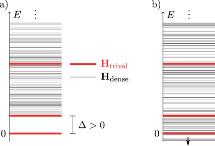
Figure 1: Competing spectra of gapless versus gapped phase for the Hamiltonian $\mathbf{H}=(\mathbf{H}_{C}+\mathbf{H}_{\mathrm{dense}})\oplus 0+0\oplus\mathbf{H}_{\mathrm{trivial}}$. a) The system is gapped with $\Delta>0$ and unique product ground state. The thermodynamic limit is in a gapped phase. b) If and only if the encoded universal Turing machine halts, there exists a critical threshold system size after which the dense spectrum of $\mathbf{H}_{C}+\mathbf{H}_{\mathrm{dense}}$ is pulled towards $-\infty$ as the system size increases, covering up the gap in the spectrum of $\mathbf{H}_{\mathrm{trivial}}$. The thermodynamic limit is in a gapless phase.

So where is the difficulty in extending the two-dimensional result of Cubitt et al. (2015a) to one-dimensional systems? One of the key ingredients in the 2D construction is a classical aperiodic tiling. The particular tiling used in Cubitt et al. (2015b), due to Robinson Robinson (1971), exhibits a fractal structure, i.e. a fixed density of structures at all length scales. This ingredient is crucial if one were to directly translate the original undecidability result to a one-dimensional system.

A Wang tile set  consists of a finite set of different types of square tiles, each tile type having one colour assigned to each of its four sides Wang (1961). Translated to Hamiltonians, the computational basis state at each site indicates which tile is placed there; the interactions of the corresponding tiling Hamiltonian are diagonal projectors in the computational basis; each of these projectors constrains neighbouring sites to be in states that correspond to a matching tile configuration (i.e. where two tiles can only be placed next to each other if the colours of the abutting sides match). A constant local dimension implies we can only have a constant number of tiles and thus of colors. But in 1D, as soon as any tile occurs a second time along the chain, the entire pattern that followed that tile previously can repeat indefinitely. (Conversely, just as in 2D, if any finite segment cannot be tiled, then neither can the infinite chain.) Thus the Tiling problem in 1D is known to be decidable, even by a simple algorithm.

For this reason, an underlying tile set like the Robinson tiles used in 2D—with patterns of all length scales—is impossible in 1D, under the physical constraint of retaining a finite local dimension.

Quantum mechanics can in principle circumvent this constraint, since entanglement can introduce long-range correlations, even in unfrustrated qudit chains Movassagh et al. (2010). Yet even though it is known that one can obtain correlations between far-away sites that decay only polynomially, the resulting Hamiltonians are gapless Hastings and Koma (2006); Movassagh and Shor (2016).

The key new idea is a 1D construction, which we denote the Marker Hamiltonian, that creates—within the system’s ground state—a periodic partition of the spin chain into segments, but whose length and period are related to the halting time of a Turing machine. This subtle interplay between the dynamics of a Turing machine, the periodic quantum ground state structure and the energy spectrum, plays the role of the classical aperiodic tilings of the 2D construction.

The paper is organized as follows. In Section III we present a summary of the construction and how it differs from the 2D one. In Section IV we detail the construction of the Marker Hamiltonian. In Section V we present the modifications that are required to the encoding of UTM into Hamiltonian interactions due to this modified set-up. These two components will be combined in Section VI. The main result on the undecidability of the spectral gap will be proven in Section VII. Finally we present some extensions to our result in Section VIII.

III Outline of the construction

Let us now give an outline of how we circumvent the problems in extending the 2D construction to 1D chains, and present an overview of the different elements which will be required to construct $\mathbf{h}^{(2)}(\upeta)$ and $\mathbf{h}^{(1)}(\upeta)$.

We start by presenting some background on Turing machines and the Halting problem.

III.1 Turing machines

A (classical) Turing machine is a simple model of computation consisting of an infinite “tape” divided into cells, and a “head” which steps left or right along the tape. The machine is always in one of a finite number of possible “internal states” $\{q_{i}\}_{i=1}^{Q}$. There is one special internal state, denoted $q_{f}$, which tells the machine to halt when it enters this state. Each cell can have one “symbol” written in it, from a finite set of possible symbols $\{\sigma_{i=1}^{\Sigma}\}$. A finite table of “transition rules” determine how the machine should behave for each possible combination of symbol and internal state. At each time step, the machine reads the symbol in the cell currently under the head and looks up this symbol and the current internal state in the transition rule table. The transition rule specifies a symbol to overwrite in the current cell, a new internal state to transition to, and whether to move the head left or right one step along the tape. The “input” to a Turing machine is whatever symbols are initially written on the tape, and the “output” is whatever is left written on the tape when it halts.

Despite its apparent simplicity, Turing machines can carry out any computation that it is possible to perform. Indeed, Turing constructed a universal Turing machine (UTM): a single set of transition rules that can perform any desired computation, determined solely by the input. Given an input $\upeta$ to a universal Turing machine $M$, the Halting Problem asks whether $M$ halts on input $\upeta$.

III.2 Encoding of the Halting problem

We want to construct a Hamiltonian whose spectral gap encodes the Halting Problem. More precisely, starting from a fixed UTM $M$, we want to construct the interactions $\mathbf{h}^{(2)}(\upeta)$ and $\mathbf{h}^{(1)}(\upeta)$ which define a 1D, translationally invariant, nearest-neighbour, spin chain Hamiltonian $\mathbf{H}_{N}(\upeta)=\mathbf{H}_{N}(M,\upeta)$ on the Hilbert space $\mathcal{H}=(\mathds{C}^{d})^{\otimes N}$, such that $\mathbf{H}_{N}(\upeta)$ is gapped in the limit $N\rightarrow\infty$ if $M$ halts on input $\upeta$, and gapless otherwise.

In the earlier 2D construction Cubitt et al. (2015b), this was accomplished by combining a trivial gapped Hamiltonian with one that has a dense spectrum (and thus gapless). The combined Hamiltonian has the property that the ground state energy is the smallest of the two. The dense Hamiltonian is then modified such that, if $M$ halts on input $\upeta$, its lowest eigenvalue is pushed up by a large enough constant, revealing the gap present due to the trivial Hamiltonian. In a non-Halting instance the dense spectrum Hamiltonian has the lowest ground state energy and therefore the combined Hamiltonian remains gapless.

In order to modify the dense Hamiltonian in this fashion, we have to construct a Hamiltonian whose ground state energy is dependent on the outcome of a (quantum) computation. This is possible thanks to Feynman and Kitaev’s history state construction, used ubiquitously throughout quantum complexity proofs Feynman (1985); Kitaev et al. (2002); Oliveira and Terhal (2005); Aharonov et al. (2009); Kempe et al. (2006); Gottesman and Irani (2009); Breuckmann and Terhal (2014); Bausch et al. (2017); Bausch and Piddock (2017). In brief, this construction allows one to take a circuit $C$ with gates $\mathbf{U}_{1},\ldots,\mathbf{U}_{T}$ acting on $m$ qubits, and embed it into a Hamiltonian on $n=m+\operatorname{poly}\log T$ qubits, such that the ground state is a superposition over histories of the computation, i.e. a state of the form $\left\lvert{\Psi}\right\rangle\propto\sum_{t=0}^{T}\left\lvert{t}\right\rangle\left\lvert{\psi_{t}}\right\rangle$. Every “snapshot” of the computation $\left\lvert{\psi_{t}}\right\rangle$ is entangled with a so-called clock register $\left\lvert{t}\right\rangle$. For $T$ computational steps, one can implement such a clock with a local Hamiltonian using $\operatorname{poly}\log T$ qubits. The state $\left\lvert{\psi_{0}}\right\rangle$ is thus input to the circuit, and $\left\lvert{\psi_{t}}\right\rangle=\mathbf{U}_{t}\cdots\mathbf{U}_{1}\left\lvert{\psi_{0}}\right\rangle$ is the state of the circuit after $t$ gates. A later construction due to Gottesman and Irani (2009) similarly encodes the evolution of a quantum Turing machine, instead of a quantum circuit. As the transition rules of a Turing machine do not depend on the head location, a benefit of encoding Turing machines rather than circuits is that the resulting Hamiltonians are naturally translationally invariant.

By adding a projector to “penalize” a subset of the possible outcomes of the computation, as encoded in $\left\lvert{T}\right\rangle\left\lvert{\psi_{T}}\right\rangle$, the ground state in these cases is pushed up in energy by $\Theta(T^{-2})$. We denote this circuit Hamiltonian with penalties with $\mathbf{H}_{C}=\mathbf{H}_{C}(M,\upeta)$—as it will be the only term dependent on the free parameter $\upeta$ and our chosen Turing machine $M$, set up such that $\upeta$ will serve as input to $M$—and the Hilbert space it acts on with $\mathcal{H}_{C}$. The energy shift in $\mathbf{H}_{C}$’s ground state can be exploited by combining this circuit Hamiltonian with three more Hamiltonians: $\mathbf{H}_{\mathrm{dense}}$ with a non-negative and asymptotically dense spectrum on a Hilbert space $\mathcal{H}_{\text{dense}}$, and $\mathbf{H}_{\mathrm{trivial}}$ with a trivial zero energy ground state and gap $\geq 1$, on Hilbert space $\mathcal{H}_{\text{trivial}}$. Then

$$\mathbf{H}_{N}(M,\upeta)\coloneqq(\mathbf{H}_{C}(M,\upeta)+\mathbf{H}_{\mathrm{dense}})\oplus 0+0\oplus\mathbf{H}_{\mathrm{trivial}}+\mathbf{H}_{\mathrm{guard}}$$

is defined on the overall Hilbert space

$$\mathcal{H}\coloneqq(\mathcal{H}_{C}\otimes\mathcal{H}_{\text{dense}})\oplus\mathcal{H}_{\text{trivial}}.$$

In order to ensure that the low-energy spectrum of $\mathbf{H}_{N}$ is determined either completely by $\mathbf{H}_{\mathrm{trivial}}$ or by the sum $\mathbf{H}_{C}+\mathbf{H}_{\mathrm{dense}}$, we have added another local Hamiltonian $\mathbf{H}_{\mathrm{guard}}$ acting on $\mathcal{H}$ with Ising-type couplings that penalize states with “mixed” support (explicitly spelled out in Theorem 25).

If the computation output in $\mathbf{H}_{C}$ is penalized, the dense spectrum is pushed up, which in turn unveils the constant spectral gap of some trivial Hamiltonian $\mathbf{H}_{\mathrm{trivial}}$, as shown in Fig. 1.

Yet even though we can easily penalize an embedded Turing machine reaching a halting state in this way (i.e. by adding a penalty term for the head being in any terminating state $q_{f}$), a history state Hamiltonian is insufficient for the undecidability proof. i) The energy penalty decreases as the embedded computation becomes longer Bausch and Crosson (2018). However, we require a constant energy penalty density across the spin chain. ii) If we try to circumvent this problem by subdividing the tape to spawn multiple copies of the Turing machine, we need to know the space required beforehand in which the computation halts, if it halts—which is also undecidable.

III.3 Amplifying the energy penalty

Cubitt et al. circumvent this problem by spawning a fixed density of computations across an underlying Robinson lattice. Like this, within every area $A$, the halting case obtains an energy penalty $\propto A$—the ground state energy density therefore differs by a constant for the Halting and non-Halting cases, allowing the ground state energy to diverge in the Halting case, which uncovers the spectral gap. The fractal properties of the Robinson tiling further ensure that that every possible tape length appears with a non-zero density in the large system size limit, so knowledge of the Turing machine’s required runtime space is unnecessary.

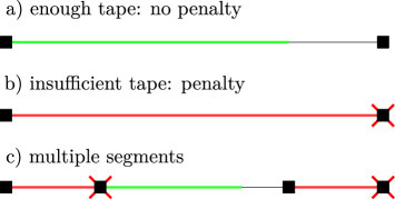
Figure 2: 1D Robinson tiling analogue, the Marker Hamiltonian: penalty between halting and not halting for the TM is flipped, i.e. we penalize not halting (the TM head moves past the available tape, or equivalently the clock driving the TM runs out of space—see Remark 19). a) If the tape—delimited by a black segment marker—is long enough for the TM to terminate, there is no penalty. b) If the tape is too short, a penalty will be inflicted due to the head running into the right segment marker. c) Mixed-length segments, each delimited with a segment marker. Those segments for which there is insufficient tape space pick up a penalty due to halting. The final construction introduces a small bonus for each segment, which shrinks the longer the segment is, and which is always smaller (in modulus) than the penalty that could be inflicted on the TM running on the available tape. In the halting case, this results in the lowest energy configuration being evenly-spaced segments with just enough tape for the TM to halt. In the non-halting case, a single segment is most favourable.

We replace the fractal Robinson tiling with a 2-local “marker” Hamiltonian $\mathbf{H}^{\prime}$ on $(\mathds{C}^{c})^{\otimes N}$, where the markers—a special spin state $\left\lvert{\raisebox{-0.5382pt}{$\blacksquare$}}\right\rangle$—bound sections of tape used for the Turing machine. $\mathbf{H}^{\prime}$ is diagonal with respect to boundary markers—i.e. $\mathbf{H}^{\prime}$ commutes with $\left\lvert{\raisebox{-0.5382pt}{$\blacksquare$}}\middle\rangle\!\middle\langle{\raisebox{-0.5382pt}{$\blacksquare$}}\right\rvert$. Thus any eigenstate $\left\lvert{\psi}\right\rangle$ has a well-defined signature with respect to these boundaries, where the signature $\operatorname{sig}\left\lvert{\psi}\right\rangle$ is defined as the binary string with 1’s where boundaries are located, and 0’s everywhere else. We construct $\mathbf{H}^{\prime}$ in such a way that two consecutive markers bounding a segment will introduce an energy bonus that falls off quickly as the length of the segment increases: e.g. any eigenstate $\left\lvert{\psi}\right\rangle$ with a signature

$$\operatorname{sig}\left\lvert{\psi}\right\rangle=(\ldots,0,\underbrace{1,0,\ldots,0,1}_{\text{length $w$}},0,\ldots)$$

will pick up a bonus of $\exp(-p(w))$ for some fixed polynomial $p$. This bonus will be strictly smaller in magnitude than any potential penalty obtained from a computation running on the same segment of length $w$, i.e. when the TM head runs out of tape (see Fig. 2).

III.4 Quantum phase estimation

To the marker Hamiltonian, we add a history state Hamiltonian $\mathbf{H}_{\text{prop}}(\phi,M)$. Here

$$\phi=\phi(\upeta)=0.\upeta_{1}1\upeta_{2}1\ldots\upeta_{|\upeta|}00\ldots$$ (4)

encodes an input parameter $\upeta\in\mathds{N}$ with $|\upeta|$ binary digits as binary fraction, where the digits of $\upeta$ are interleaved by $1$s. The second parameter $M$ is a classical universal Turing machine. We construct $\mathbf{H}_{\text{prop}}$ to encode the following computation:

1. A Quantum Turing machine performs quantum phase estimation (QPE) on a single-qubit unitary that encodes the input $\phi$.

2. The classical universal TM $M$ uses the binary expansion of $\phi$ as input and performs a computation on it.

Up to a slight modification for 1. which we will explain later, this is the same Turing machine construction as in (Cubitt et al., 2015b, sec. 6). The Hamiltonian $\mathbf{H}_{\text{prop}}$ is set up to spawn one instance of the computation per segment, and we penalize the TM $M$ running out of available tape up to the next boundary marker with some local terms; as before we denote the resulting local Hamiltonian with $\mathbf{H}_{C}$. We finally add a trivial Hamiltonian $\mathbf{H}_{\mathrm{trivial}}$ with ground state energy $-1$ and constant spectral gap. The overall Hamiltonian is then

$$\mathbf{H}_{N}= \beta(\mu\mathbf{H}^{\prime}+\mathbf{H}_{C}(M,\upeta)+\mathbf{H}_{\mathrm{dense}})\oplus 0$$

$$+0\oplus\mathbf{H}_{\mathrm{trivial}}+\mathbf{H}_{\mathrm{guard}},$$

where $\mu=2^{-|\phi|}$ is a small constant, defined for $\phi(\upeta)$ as given in Eq. 4 with $|\phi|=2|\upeta|$. $\beta>0$ can be chosen arbitrarily small.

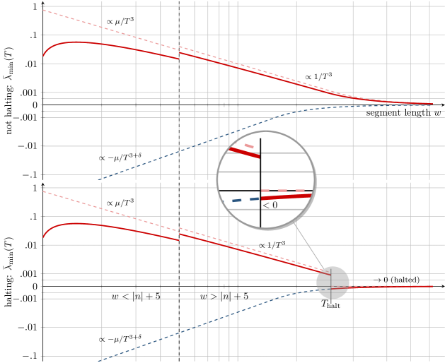
Figure 3: Energy contribution $\bar{\lambda}_{\text{min}}(T)$ from a single segment of length $w$ of the marker and TM Hamiltonian $\mu\mathbf{H}^{\prime}+\mathbf{H}_{C}$ shown in red, where $T$ is the runtime of the encoded computation, bounded either by the segment length or by the halting time of the TM. The prefactor $\mu=2^{-2|\upeta|}$ is a small constant to compensate for the fact that on too short segments the phase estimation truncates the output, which we can only penalize with strength $\Omega(\mu/T^{3})$. The dashed red line is the contribution of $\mathbf{H}_{C}$, i.e. the energy penalty inflicted in case of the Turing machine running out of space. The dashed blue line is the bonus from $\mu\mathbf{H}^{\prime}$.

We will now explain how our construction differers during the QPE step. QPE can be performed exactly when there is sufficient tape Nielsen and Chuang (2010). In case there is insufficient space for the full binary expansion of the input parameter $\phi$, the output is truncated, and the resulting output state is not necessarily a product state in the computational basis anymore.

As in the 2D model, we have to allow for the possibility that the QPE truncates $\phi$, possibly resulting in the universal TM dovetailed to the QPE switching its behavior to halting. In the 2D construction of Cubitt et al. (2015b), one could circumvent this by simply subtracting off the energy contribution from truncated phase-estimation outputs; yet we cannot use this mechanism in our result, since it is not possible in the 1D construction, since we cannot à priori know the length of the segments on which the Turing machine runs. Instead, we augment the QPE algorithm by a short program which verifies that the expansion has been performed in full, and otherwise inflicts a large enough energy penalty to offset the case that the UTM now potentially halts on the perturbed QPE output.

To this end, we make use of the specific encoding of $\phi$: the interleaved $1$s are flags indicating how many digits to expand. Like this, before the inverse quantum Fourier transform, we know that the least-significant qubit is exactly in state $\left\lvert{+}\right\rangle$ if the expansion was completed, and has overlap at least $\mu=2^{-|\phi|}$ with $\left\lvert{-}\right\rangle$ otherwise. By adding a penalty term to the Hamiltonian for said digit in state $\left\lvert{-}\right\rangle$, we can penalize those segments with insufficient tape for a full expansion of the input, independently of whether the universal TM then halts or not on a faulty input. This result manifests as a kink of the lower energy bound for a too-short segment of length $w$ in Fig. 3. Yet since the marker Hamiltonian $\mathbf{H}^{\prime}$ is attenuated by $\mu$ as well, the energy remains nonnegative throughout for these segments. Therefore, the only segments left to be analyzed are those for which the input can be assumed un-truncated.

III.5 Ground state energy analysis

When there is enough space for the QPE to be permormed, there are two possibilities for the ground state energy of $\mathbf{H}_{N}$. In case $M(\phi)$ does not halt, any instance of the TM running on any tape length will run out of tape space, incurring the penalty explained in Fig. 2. This halting penalty will always dominate the bonus coming from the segment length, and we show the ground state energy to be $\lambda_{\text{min}}(\mathbf{H}_{N})\geq 0$. In case the TM does halt, there will be minimal segment length $w_{\text{halt}}$ above which segments will not pick up the penalty from exhausting the tape. Since the bonus given by the Marker Hamiltonian is decreasing with increasing segment length, the optimal energy configuration will therefore be achieved by partitioning the whole chain into segments of length $w_{\text{halt}}$, each of which picks up a tiny—but finite—negative energy contribution. We prove $\lambda_{\text{min}}(\mathbf{H}_{N})<-\lfloor N/w_{\text{halt}}\rfloor\Omega(1/T_{\text{halt}}^{3})$ in that case, where $T_{\text{halt}}$ is the number of computation steps till halting. As the system size $N$ increases, the ground state energy will therefore diverge to $-\infty$.

The the claims of Theorem 1 will then follow by combining the construction outlined with a trivial, gapped Hamiltonan and a dense spectrum, gapless Hamiltonian. The dense spectrum Hamiltonian will be modified to have ground state energy determined by the outcome of the computation of the QTM running on the tape segments defined by the Marker Hamitonian, so that the low-energy part of the spectum of the combined Hamiltonian will be gapped or gapless depending on whether the UTM halts or not.

IV Marker Tiling

In this section we will give an explicit construction of the Marker Hamiltonian.

IV.1 Concept

Figure 4: 2D Robinson tiling construction with instances of a Turing machine running on the upper edges of the fractal rectangles. Each edge represents the available tape for the Turing machine. In the non-halting case a), there will never be any halting penalty, no matter how much tape there is available. In the halting case b), there is a threshold side length after which each rectangle larger than the threshold contributes a penalty (red)—which yields a small but nonzero ground state energy density; the ground state energy diverges.
In the 1D case we show the segments emerging from the Marker Hamiltonian from Section IV (cf. Fig. 2). In the non-halting case c), no segment length is long enough to contain the entire computation; all segments obtain a penalty (red). In the halting case d), there is an ideal segment length (green) with just enough tape tor the TM to halt; as per Fig. 3, this segment has the maximum possible bonus. Segments too short (red) contribute a net energy penalty, whereas segments too long (magenta) do contribute a bonus, yet not one as large as the optimal segment length.

In order to spawn a fixed density of computations in 1D without the aid of a fractal underlying structure, we need to know an optimal segment length to subdivide the spin chain into. In the halting case, this should be just enough tape for the computation to terminate. However, if we aim to construct a reduction from the Halting Problem, we cannot know the space required beforehand—which, in particular, could be uncomputably large, or infinite! One way out is to spawn Turing machines on tapes of all possible lengths, and do this with a fixed density. In 2D this can be achieved using an underlying fractal tiling such as that due to Robinson Robinson (1971), see Fig. 4.

The two-dimensional construction thus crucially depends on one’s ability to create structures of all length scales, in order to define “lines” of all sizes , which are then used as a tape for running a Quantum Turing machine: the key property of the fractal which makes the construction work is that every possible tape length indeed appears with a non-zero density in the large system size limit.

As already mentioned, constructing a fractal tiling with a fixed density of structures of all length scales seems impossible in one dimension. We therefore replace the fractal Robinson tiling with a “marker” Hamiltonian, where the markers bound sections of tape used for the Turing machine (just like the lower boundaries of the squares in Fig. 4). We will construct the Hamiltonian in such a way that two consecutive markers bounding a segment will introduce an energy bonus that falls off quickly as the length of the segment increases. This bonus will be weak enough to permit an executing QTM to “extend” the tape as needed, in the sense that the bonus due to the marker boundaries is strictly smaller in magnitude than the potential penalty introduced when the QTM head runs out of tape (see Fig. 2).

IV.2 The Marker Hamiltonian

We now construct the Marker Hamiltonian. It will be a local Hamiltonian $\mathbf{H}$ on a chain of qudits with a special spin state $\left\lvert{\raisebox{-0.5382pt}{$\blacksquare$}}\right\rangle$, which we call a boundary, and which will separate the different tape segments. For a product state $\left\lvert{\psi}\right\rangle$, we define a signature with respect to these boundaries as the binary string with 1’s where boundaries are located, and 0’s everywhere else, which we will denote by $\operatorname{sig}\left\lvert{\psi}\right\rangle$. The Hamiltonian we construct will leave the signature invariant, i.e. $\operatorname{sig}\left\lvert{\psi}\right\rangle=\operatorname{sig}\mathbf{H}\left\lvert{\psi}\right\rangle$ for all $\left\lvert{\psi}\right\rangle$. This property allows us to block-diagonalize $\mathbf{H}$ with respect to states of the same signature. For a given block signature, say $(1,0,0,0,1,0,0,1)$, the Hamiltonian gives an energy bonus (i.e. a negative energy contribution) to each $1$-bounded segment, which is large when the boundary markers are close, and becomes smaller the longer the segment. This introduces a notion of boundaries that are “attracted” to each other, and our goal is to have a falloff as $\sim-1/g(l)$ in the segment’s length $l$, where $g$ is a function we can choose. In brief, “attraction”, in this context, simply means that the energy bonus given by $\mathbf{H}$ to pairs of boundary symbols grows the closer they are to each other.

For reasons of clarity, we start by constructing a Hamiltonian where the falloff is a fixed function $g$ that is asymptotically bounded as $\Omega(2^{l})\leq g\leq\operatorname{O}(4^{l})$. In a second step, we allow the falloff to be tuned, replacing $l$ by an arbitrary exponential in $l$, such that the falloff is doubly exponential in the segment length.

IV.3 Construction

We start with the following lemma.

Lemma 2.

Let $\mathcal{H}\coloneqq(\mathds{C}^{3})^{\otimes N}$ be a chain of qutrits of length $N$ with local computational basis $\{\left\lvert{\raisebox{-0.5382pt}{$\blacksquare$}}\right\rangle,\left\lvert{\raisebox{0.43057pt}{$\vartriangleright$}}\right\rangle,\left\lvert{\raisebox{0.43057pt}{$\blacktriangleright$}}\right\rangle\}$, and for a product state $\left\lvert{\psi}\right\rangle\in\mathcal{H}$, $\left\lvert{\psi}\right\rangle=\left\lvert{\psi_{1}}\right\rangle\cdots\left\lvert{\psi_{N}}\right\rangle$, we define a “boundary signature” $\operatorname{sig}\left\lvert{\psi}\right\rangle=(\left\langle{\raisebox{-0.5382pt}{$\blacksquare$}}\middle|{\psi_{1}}\right\rangle,\ldots,\left\langle{\raisebox{-0.5382pt}{$\blacksquare$}}\middle|{\psi_{N}}\right\rangle)$, extended linearly to $\mathcal{H}$. Define two local Hamiltonian terms

$$\mathbf{h}_{1} \coloneqq\left\lvert{\raisebox{0.43057pt}{$\blacktriangleright$}}\middle\rangle\!\middle\langle{\raisebox{0.43057pt}{$\blacktriangleright$}}\right\rvert\otimes\big{(}\left\lvert{\raisebox{0.43057pt}{$\vartriangleright$}\raisebox{0.43057pt}{$\vartriangleright$}}\right\rangle-\left\lvert{\raisebox{0.43057pt}{$\blacktriangleright$}\raisebox{0.43057pt}{$\vartriangleright$}}\right\rangle\big{)}\big{(}\left\langle{\raisebox{0.43057pt}{$\vartriangleright$}\raisebox{0.43057pt}{$\vartriangleright$}}\right\rvert-\left\langle{\raisebox{0.43057pt}{$\blacktriangleright$}\raisebox{0.43057pt}{$\vartriangleright$}}\right\rvert\big{)}$$

$$\mathbf{h}_{2} \coloneqq\big{(}\left\lvert{\raisebox{0.43057pt}{$\blacktriangleright$}\raisebox{0.43057pt}{$\vartriangleright$}}\right\rangle-\left\lvert{\raisebox{0.43057pt}{$\blacktriangleright$}\raisebox{0.43057pt}{$\blacktriangleright$}}\right\rangle\big{)}\big{(}\left\langle{\raisebox{0.43057pt}{$\blacktriangleright$}\raisebox{0.43057pt}{$\vartriangleright$}}\right\rvert-\left\langle{\raisebox{0.43057pt}{$\blacktriangleright$}\raisebox{0.43057pt}{$\blacktriangleright$}}\right\rvert\big{)}\otimes\left\lvert{\raisebox{-0.5382pt}{$\blacksquare$}}\middle\rangle\!\middle\langle{\raisebox{-0.5382pt}{$\blacksquare$}}\right\rvert$$

and set $\mathbf{h}_{\mathrm{walk}}\coloneqq\mathbf{h}_{1}+\mathbf{h}_{2}$. Let

$$\mathbf{p} \coloneqq 2\left\lvert{\raisebox{-0.5382pt}{$\blacksquare$}\raisebox{-0.5382pt}{$\blacksquare$}}\middle\rangle\!\middle\langle{\raisebox{-0.5382pt}{$\blacksquare$}\raisebox{-0.5382pt}{$\blacksquare$}}\right\rvert+2\left\lvert{\raisebox{0.43057pt}{$\vartriangleright$}\raisebox{0.43057pt}{$\blacktriangleright$}}\middle\rangle\!\middle\langle{\raisebox{0.43057pt}{$\vartriangleright$}\raisebox{0.43057pt}{$\blacktriangleright$}}\right\rvert+2\left\lvert{\raisebox{-0.5382pt}{$\blacksquare$}\raisebox{0.43057pt}{$\vartriangleright$}}\middle\rangle\!\middle\langle{\raisebox{-0.5382pt}{$\blacksquare$}\raisebox{0.43057pt}{$\vartriangleright$}}\right\rvert$$

Then

$$\mathbf{H}_{\mathrm{walk}}+\mathbf{P}\coloneqq \sum_{i=1}^{N-2}\mathds{1}_{\{1,\ldots,i-1\}}\otimes\mathbf{h}_{\mathrm{walk}}\otimes\mathds{1}_{\{i+3,\ldots,N\}}$$

$$+ \sum_{i=1}^{N-1}\mathds{1}_{\{1,\ldots,i-1\}}\otimes\mathbf{p}\otimes\mathds{1}_{\{i+2,\ldots,N\}}$$

is a 3-local Hamiltonian which is positive semi-definite, and block-diagonal with respect to the subspaces spanned by states with identical signature $\operatorname{sig}$.

Proof.

The first two claims are true by construction. The Hamiltonian $\mathbf{H}_{\text{walk}}+\mathbf{P}$ is further block-diagonal with respect to $\operatorname{sig}$ because $\operatorname{sig}(\mathbf{H}_{\text{walk}}+\mathbf{P})\left\lvert{\psi}\right\rangle=\operatorname{sig}\left\lvert{\psi}\right\rangle\ \forall\left\lvert{\psi}\right\rangle\in\mathcal{H}$, as none of the local terms ever affect the subspaces spanned by the boundary symbol $\left\lvert{\raisebox{-0.5382pt}{$\blacksquare$}}\right\rangle$. ∎

As a second step, we employ a boundary trick by Gottesman and Irani (2009) to ensure that blocks not terminated by a boundary marker have a ground state energy at least $2$ higher than $\blacksquare$-terminated blocks. It is worth emphasizing that this is not achieved by a term that only acts on the boundary, but in a translationally-invariant way, i.e. by adding the same one- and two-local terms throughout the chain. In brief, it exploits the fact that while there are $N$ spins in the chain, there is only $N-1$ edges between them. We state this rigorously in the following remark.

Remark 3 (Gottesman and Irani (2009)).

Give an energy bonus of strength 4 to $\left\lvert{\raisebox{-0.5382pt}{$\blacksquare$}}\right\rangle$, and an energy penalty of $2$ to $\left\lvert{\raisebox{-0.5382pt}{$\blacksquare$}}\right\rangle$ appearing next to any symbol (including $\blacksquare$ itself. I.e. if $\left\lvert{\raisebox{-0.5382pt}{$\blacksquare$}}\right\rangle$ appears at the end of the chain there will be a net bonus of $2$, otherwise a net penalty of zero). Collect these terms in a Hamiltonian $\mathbf{P}^{\prime}$. Then, apart from positive semi-definiteness,

$$\mathbf{H}\coloneqq\mathbf{H}_{\text{walk}}+\mathbf{P}+\mathbf{P}^{\prime}$$ (5)

where $\mathbf{H}_{\text{walk}}$ and $\mathbf{P}$ are defined in Lemma 2, has the same properties claimed in Lemma 2, but any block not terminated by a boundary will have energy $\geq-2$, while all properly-terminated blocks will have a ground state energy $-4$.

Proof.

The first claim is straightforward, as $\mathbf{P}^{\prime}$ does not change the interaction structure of $\mathbf{H}$. The last claim follows from the fact that the only way of obtaining a net bonus is to place a boundary symbol at the end of the spin chain, where it picks up a net bonus of $2$. The maximum possible bonus of any state is thus $4$, which will be achieved by signatures that are properly bounded on either side. ∎

From now on, when we talk of “properly bounded”, we always mean a signature with boundary blocks $\blacksquare$ at each end. Individual cases where only one side carries a boundary will be mentioned as such explicitly then.

IV.4 Spectral Analysis

In the following, the “good” blocks will therefore be those that have ground space energy $-4$, all of which aFre properly bounded. Remark 3 allows us to analyze the blocks more closely, which we do in the following lemma.

Lemma 4.

Let $\mathbf{H}=\mathbf{H}_{\text{walk}}+\mathbf{P}+\mathbf{P}^{\prime}$ be as in Eq. 5. If we write $\mathbf{H}=\bigoplus_{s\in\{0,1\}^{N}}\mathbf{H}_{s}$ as the block-decomposition of $\mathbf{H}$, where $s$ denotes an arbitrary length $N$ binary string, then every properly bounded block will either

1. have two consecutive boundaries, and thus a ground state energy $\geq-2$, or

2. have signature of consecutive $1$-bounded segments of $0$s. In this case, $\mathbf{H}_{s}$ further block-diagonalizes into $\mathbf{H}_{s}=\mathbf{G}_{s}\oplus\mathbf{R}_{s}$, where $\mathbf{R}_{s}$ is within the span of states penalized by $\mathbf{P}$ in Lemma 2, and $\mathbf{G}_{s}$ in its kernel.

3. The ground state energy of $\mathbf{R}_{s}$ is $\geq-2$.

4. The ground state energy of $\mathbf{G}_{s}$ equals $-4$, and $\mathbf{G}_{s}$ will be a sum of terms of the form $\mathds{1}_{\{1,\ldots,l\}}\otimes\Delta_{w}\otimes\mathds{1}_{\{l+w+1,\ldots,N\}}$, where $\Delta_{w}$ is the Laplacian of a path graph of length $w$ (i.e. a graph with vertices $\{1,\ldots,w\}$ and edges $\{(i,i+1):i=1,\ldots,w-1\}$). Here $l$ and $w$ depend on the signature $s$—more precisely, for every contiguous section of $0$s in $s$ surrounded by a pair of $1$s, $l$ marks the left $1$ and $w$ is the length of the section of $0$s.

Proof.

If there are two neighbouring $1$s in the signature $s$, the penalty term $\left\lvert{\raisebox{-0.5382pt}{$\blacksquare$}\raisebox{-0.5382pt}{$\blacksquare$}}\middle\rangle\!\middle\langle{\raisebox{-0.5382pt}{$\blacksquare$}\raisebox{-0.5382pt}{$\blacksquare$}}\right\rvert$ picks up an energy contribution of 2. Since $\mathbf{H}_{\mathrm{prop}}$ is already positive semi-definite and block-diagonal with respect to signatures, any state $\left\lvert{\psi}\right\rangle$ with support fully contained in the block corresponding to signature $s$ must thus necessarily satisfy $\left\langle{\psi}\right\rvert\mathbf{H}\left\lvert{\psi}\right\rangle\geq\left\langle{\psi}\right\rvert\mathbf{P}\left\lvert{\psi}\right\rangle\geq 2$. The first claim follows.

So let us assume that all $1$s are spaced away from each other with at least one $0$. Within the 2-dimensional $0$ subspace spanned by the local basis states $\left\lvert{\raisebox{0.43057pt}{$\blacktriangleright$}}\right\rangle$ and $\left\lvert{\raisebox{0.43057pt}{$\vartriangleright$}}\right\rangle$. We note that the penalized substring $\left\lvert{\raisebox{0.43057pt}{$\vartriangleright$}\raisebox{0.43057pt}{$\blacktriangleright$}}\right\rangle$ is also an invariant, meaning that no transition rule can create or destroy this configuration. Any state that, when expanded in the computational basis, has at least one expansion term with said substring will thus necessarily have all terms with this specific substring. The same arguments holds for the invariant substring $\left\lvert{\raisebox{-0.5382pt}{$\blacksquare$}\raisebox{0.43057pt}{$\vartriangleright$}}\right\rangle$, and the second claim follows.

Since any eigenstate of $\mathbf{R}_{s}$ picks up the full penalty contribution of $2$, the third claim follows.

If neither of the invariant substrings $\left\lvert{\raisebox{0.43057pt}{$\vartriangleright$}\raisebox{0.43057pt}{$\blacktriangleright$}}\right\rangle$ and $\left\lvert{\raisebox{-0.5382pt}{$\blacksquare$}\raisebox{0.43057pt}{$\vartriangleright$}}\right\rangle$ occur, we can assume that all $1$-bounded segments of $0$s lie within the span of the states

$$\left\lvert{\raisebox{0.43057pt}{$\blacktriangleright$}\raisebox{0.43057pt}{$\vartriangleright$}\raisebox{0.43057pt}{$\vartriangleright$}\cdots\raisebox{0.43057pt}{$\vartriangleright$}\raisebox{0.43057pt}{$\vartriangleright$}}\right\rangle,\left\lvert{\raisebox{0.43057pt}{$\blacktriangleright$}\raisebox{0.43057pt}{$\blacktriangleright$}\raisebox{0.43057pt}{$\vartriangleright$}\cdots\raisebox{0.43057pt}{$\vartriangleright$}\raisebox{0.43057pt}{$\vartriangleright$}}\right\rangle,\ldots$$

$$\ldots,\left\lvert{\raisebox{0.43057pt}{$\blacktriangleright$}\raisebox{0.43057pt}{$\blacktriangleright$}\raisebox{0.43057pt}{$\blacktriangleright$}\cdots\raisebox{0.43057pt}{$\blacktriangleright$}\raisebox{0.43057pt}{$\vartriangleright$}}\right\rangle,\left\lvert{\raisebox{0.43057pt}{$\blacktriangleright$}\raisebox{0.43057pt}{$\blacktriangleright$}\raisebox{0.43057pt}{$\blacktriangleright$}\cdots\raisebox{0.43057pt}{$\blacktriangleright$}\raisebox{0.43057pt}{$\blacktriangleright$}}\right\rangle.$$ (6)

Since there is no penalty acting on any of those states, the ground state energy of $\mathbf{G}_{s}$ equals $-4$.

Each such segment of contiguous $0$s thus defines a separate path graph, where the vertices are precisely these states, linked by the transition rules given in $\mathbf{H}_{\mathrm{walk}}$ in Lemma 2. Denote the path graphs corresponding to these segments with $G_{1},\ldots,G_{n}$, where we assume that there are $n$ 1-bounded segments of 0s in signature $s$. As each segment is independent of the others, the overall graph spanned by these individual paths is the Cartesian product of the individual paths, i.e. $G=G_{1}\square G_{2}\square\ldots\square G_{n}$. This is precisely a hyperlattice with side lengths uniquely determined by the lengths of the individual segments.

The transition rules in $\mathbf{h}_{\mathrm{walk}}$ therefore result in a block $\mathbf{G}_{s}=\Delta_{G}$, i.e. the Hamiltonian is precisely the Laplacian of the graph of determined by the transition rules (for an extensive analysis see e.g. Bausch et al. (2017)). We further know that the Laplacian of a Cartesian product of graphs decomposes as

$$\Delta(G) =\Delta(G_{1})\otimes\mathds{1}\otimes\ldots\otimes\mathds{1}$$

$$+\mathds{1}\otimes\Delta(G_{2})\otimes\mathds{1}\otimes\ldots\otimes\mathds{1}+\ldots$$

$$\ldots +\mathds{1}\otimes\ldots\otimes\mathds{1}\otimes\Delta(G_{n}),$$ (7)

and the last claim follows. ∎

A more direct route to Eq. 7 is to note that $\mathbf{H}_{\mathrm{walk}}$ is by definition the Laplacian of a graph with vertices given by strings of the alphabet $\{\raisebox{-0.5382pt}{$\blacksquare$},\raisebox{0.43057pt}{$\vartriangleright$},\raisebox{0.43057pt}{$\blacktriangleright$}\}$, and edges by the transition rules in Lemma 2. Those connected graph components that do not carry a penalty due to an invalid configuration (which either holds for all vertices, or none) are lattices in $n$ dimensions—where $n$ is the number of $1$-bounded segments—and side lengths determined by the segments’ lengths. Eq. 7 is precisely the Laplacian of this grid graph.

For the sake of clarity, we will keep calling the segments of consecutive zeros bounded by $\blacksquare$ on either side “$1$-bounded segments”, and when talking about the entire string we use the term “properly bounded”. We will henceforth re-label the states in Eq. 6 as $\left\lvert{1}\right\rangle,\ldots,\left\lvert{w}\right\rangle$, where $w$ denotes the length of the segment. Our next step will be to add a 2-local bonus term which gives an energy bonus to the arrow appearing to the left of the boundary, i.e. to $\left\lvert{\raisebox{0.43057pt}{$\blacktriangleright$}\raisebox{-0.5382pt}{$\blacksquare$}}\right\rangle$.

Lemma 5.

Define $\mathbf{H}^{\prime}\coloneqq\mathbf{H}+\mathbf{P}^{\prime\prime}+\mathbf{B}$, where

• $\mathbf{H}$ is taken from Eq. 5,

• $\mathbf{P}^{\prime\prime}=1/2\sum_{i=1}^{N}\left\lvert{\raisebox{-0.5382pt}{$\blacksquare$}}\middle\rangle\!\middle\langle{\raisebox{-0.5382pt}{$\blacksquare$}}\right\rvert_{i}$ gives a penalty of $1/2$ to any boundary term, and

• $\mathbf{B}=-\sum_{i=1}^{N-1}\left\lvert{\raisebox{0.43057pt}{$\blacktriangleright$}\raisebox{-0.5382pt}{$\blacksquare$}}\middle\rangle\!\middle\langle{\raisebox{0.43057pt}{$\blacktriangleright$}\raisebox{-0.5382pt}{$\blacksquare$}}\right\rvert_{i,i+1}$ gives a bonus of 1 to states where the arrow has reached the right boundary.

Then

1. $\mathbf{H}^{\prime}$ is still 3-local and block-diagonal in signatures, i.e. $\mathbf{H}^{\prime}\coloneqq\sum_{s}\mathbf{H}^{\prime}_{s}$. If $s$ is properly bounded and has no double $11$s, the corresponding block decomposes as $\mathbf{H}^{\prime}_{s}=\mathbf{G}^{\prime}_{s}\oplus\mathbf{R}^{\prime}_{s}$ similar to Lemma 4, but such that the primed versions carry the extra penalties and bonus terms.

2. For any such $s$, $\mathbf{R}^{\prime}_{s}\geq\mathbf{G}^{\prime}_{s}+2$.

3. $\mathbf{G}^{\prime}_{s}$ breaks up into sum of terms of the form $\mathds{1}\otimes\Delta^{\prime}_{w}\otimes\mathds{1}$, where $\Delta^{\prime}_{w}$ is a perturbed path graph Laplacian $\Delta^{\prime}_{w}\coloneqq\Delta_{w}-\left\lvert{w}\middle\rangle\!\middle\langle{w}\right\rvert$ (where $\left\lvert{w}\right\rangle$ labels the last of the basis states given in Eq. 6, as mentioned).

Proof.

The first two claims follow immediately from Lemma 4, since all of the newly-introduced terms leave signatures and penalized substrings invariant, and are at most 2-local.

Since the Cartesian graph product is associative and commutative, it is enough to show the decomposition for the case of two graphs $G_{1}$ and $G_{2}$, and a single vertex $v\in G_{1}$ which we want to give a bonus of $-1$ to. Denote the bonus matrix for $G_{1}$ with $\mathbf{B}_{1}$. We have that the adjacency matrix $\mathbf{A}_{G_{1}\square G_{2}}=\mathbf{A}_{G_{1}}\otimes\mathds{1}+\mathds{1}\otimes\mathbf{A}_{G_{2}}$. Vertex $v$ is thus mapped to a family of product vertices $(v,v^{\prime})_{v^{\prime}\in G_{2}}$, which are precisely the corresponding bonus’ed vertices in $G=G_{1}\square G_{2}$ that have to receive a bonus of $-1$. The bonus term for $G$ is thus $\mathbf{B}=\mathbf{B}_{1}\otimes\mathds{1}$, and the claim follows. ∎

We know that any Laplacian eigenvalues $\mu,\nu$ of two graphs $G_{1},G_{2}$ combine to a Laplacian eigenvalue $\mu+\nu$ of $G_{1}\square G_{2}$ (see e.g. (Brouwer and Haemers, 2011, Ch. 1.4.6)). It is straightforward to extend this fact to the case of bonus’ed graphs, which will allow us to analyse the spectrum of each signature block $\mathbf{H}^{\prime}_{s}$.

The reader will have noticed that in contrast to Lemma 4, Lemma 5 does not make any claims about the ground state energy of the individual blocks. Naïvely, one could assume that the ground state energy of each block will diverge to $+\infty$ with the number of boundaries present, as each of them carries a penalty of $+1/2$—but how does this balance with the bonus of $-1$, which we apply to only a single basis state in the graph Laplacian’s ground space, and not on each vertex?

In order to answer this question, let us step back for a moment and develop a bound for the lowest eigenvalue of a modified path graph Laplacian $\Delta^{\prime}_{w}$. We will do this in a series of technical lemmas.

Lemma 6.

$\Delta^{\prime}_{w}$ has precisely one negative eigenvalue.

Proof.

Assume this is not the case. Then there exist at least two eigenvectors $\left\lvert{u}\right\rangle,\left\lvert{v}\right\rangle$ with negative eigenvalues, and any $\left\lvert{x}\right\rangle\in\operatorname{span}\{\left\lvert{u}\right\rangle,\left\lvert{v}\right\rangle\}$ satisfies $\left\langle{x}\right\rvert\Delta^{\prime}_{w}\left\lvert{x}\right\rangle<0$. Since $\dim\ker\left\lvert{w}\middle\rangle\!\middle\langle{w}\right\rvert=w-1$, there exists a nonzero $\left\lvert{x}\right\rangle\in\operatorname{span}\{\left\lvert{u}\right\rangle,\left\lvert{v}\right\rangle\}$ such that $\left\lvert{w}\middle\rangle\!\middle\langle{w}\right\rvert\left\lvert{x}\right\rangle=0$. Therefore $0>\left\langle{x}\right\rvert\Delta^{\prime}_{w}\left\lvert{x}\right\rangle=\left\langle{x}\right\rvert\Delta_{w}\left\lvert{x}\right\rangle$, contradiction, since $\Delta_{w}$ is positive semi-definite. ∎

As a next step, we will lower-bound the minimum eigenvalue of $\Delta^{\prime}_{w}$.

Lemma 7.

The minimum eigenvalue of $\Delta^{\prime}_{w}$ satisfies $\lambda\geq-1/2-2^{-w}$.

Proof.

We first observe that $\Delta^{\prime}_{w}$ is tridiagonal, e.g.

$$\Delta^{\prime}_{5}=\begin{pmatrix}1&-1&0&0&0\\ -1&2&-1&0&0\\ 0&-1&2&-1&0\\ 0&0&-1&2&-1\\ 0&0&0&-1&0\end{pmatrix}.$$

We can thus expand the determinant $p_{w}(\lambda)\coloneqq\det(\Delta^{\prime}_{w}-\lambda\mathds{1})$ using the continuant recurrence relation (see (Muir, 1882, Ch. III))

$$f_{0} \coloneqq 1$$

$$f_{1} \coloneqq\lambda-1$$

$$f_{i} \coloneqq(\lambda-2)f_{i-1}-f_{i-2}$$

$$p_{w}(\lambda) \coloneqq\lambda f_{w-1}-f_{w-2}$$

As can be easily verified, a solution to this relation is given by the expression

$$p_{w}(\lambda)=-\frac{2^{-w-1}}{\sqrt{\lambda-4}}\left(3\sqrt{\lambda}z_{w}^{-}(\lambda)+\sqrt{\lambda-4}z_{w}^{+}(\lambda)\right)$$ (8)

where $z_{w}^{+}(\lambda)\coloneqq x_{w}(\lambda)+y_{w}(\lambda)$, $z_{w}^{-}(\lambda)\coloneqq x_{w}(\lambda)-y_{w}(\lambda)$, and

$$x_{w}(\lambda) =\left(\lambda-\sqrt{\lambda-4}\sqrt{\lambda}-2\right)^{w}$$

$$y_{w}(\lambda) =\left(\lambda+\sqrt{\lambda-4}\sqrt{\lambda}-2\right)^{w}.$$

There is of course no hope to resolve $p_{w}(\lambda)=0$ for $\lambda$ directly, so we go a different route. First note that $p_{w}(\lambda)$ is necessarily analytic, since it is the characteristic polynomial of $\Delta^{\prime}_{w}$. We can calculate $p_{w}(-1/2)=(-1)^{1+w}2^{-w},$ and thus know that $\operatorname{sign}p_{w}(-1/2)=1$ for $w$ odd, and $-1$ for $w$ even. If we can show that $p_{w}(-1/2-1/2^{w})$ has the opposite sign, then by the intermediate value theorem we know there has to exist a root on the interval $[-1/2-1/2^{w},-1/2]$, and the claim follows.

First substitute $p_{w}(-1/2-1/2^{w})=:A_{w}/B_{w}$, where

$$B_{w} =2^{w+1}\sqrt{2^{-w}+\frac{9}{2}},$$

$$A_{w} =-a_{1,w}(x^{\prime}_{w}-y^{\prime}_{w})-a_{2,w}(x^{\prime}_{w}+y^{\prime}_{w}),$$

$$a_{1,w} =3\sqrt{2^{-w}+\frac{1}{2}},$$

$$a_{2,w} =\sqrt{2^{-w}+\frac{9}{2}},$$

$$x^{\prime}_{w} =\left(\sqrt{2^{-w}+\frac{9}{2}}\sqrt{2^{-w}+\frac{1}{2}}-2^{-w}-\frac{5}{2}\right)^{w},$$

$$y^{\prime}_{w} =\left(-\sqrt{2^{-w}+\frac{9}{2}}\sqrt{2^{-w}+\frac{1}{2}}-2^{-w}-\frac{5}{2}\right)^{w}.$$

Then $B_{w}$, $a_{1,w}$ and $a_{2,w}$ are real positive for all $w$. We distinguish two cases.

w even.

If $w$ is even, we need to show $p_{w}(-1/2-1/2^{w})\geq 0$, which is equivalent to

$$0\leq\frac{A_{w}}{B_{w}}$$

$$\Longleftrightarrow\quad 0\leq A_{w}=-a_{1,w}(x^{\prime}_{w}-y^{\prime}_{w})-a_{2,w}(x^{\prime}_{w}+y^{\prime}_{w})$$

$$\Longleftrightarrow\quad 0\geq a(x^{\prime}_{w}-y^{\prime}_{w})+(x^{\prime}_{w}+y^{\prime}_{w})$$

$$\Longleftrightarrow\quad \frac{a-1}{a+1}y^{\prime}_{w}\geq x^{\prime}_{w},$$

where we defined $a\coloneqq a_{1,w}/a_{2,w}\in[1,2]$. Now, for $w$ even, $y^{\prime}_{w}\geq x^{\prime}_{w}$, so it suffices to show

$$\frac{a-1}{a+1}\left(\frac{5}{2}+\frac{3}{2}\right)^{w}\geq\left(\frac{5}{2}-\frac{3}{2}\right)^{w}\quad\Longleftrightarrow\quad\frac{a-1}{a+1}\geq\frac{1}{4^{w}},$$

which is true for all $w\geq 2$.

w odd.

Unlike the even case now we have $y^{\prime}_{w}\leq x^{\prime}_{w}$, and it suffices to show

$$\frac{a-1}{a+1}\left(\frac{5}{2}\right)^{w}\leq\left(\frac{5}{2}\right)^{w}\quad\Longleftrightarrow\quad\frac{a-1}{a+1}\leq 1,$$

which also holds true for all $w\geq 0$. This finishes the proof. ∎

And finally, using a similar approach, we will obtain an upper bound for the minimum eigenvalue of $\Delta^{\prime}_{w}$.

Lemma 8.

The minimum eigenvalue of $\Delta^{\prime}_{w}$ satisfies $\lambda\leq-1/2-4^{-w}$.

Proof.

The idea is to extend the area around $-1/2$ for which $p_{w}$ is positive for $w$ odd, and negative for $w$ even, respectively. We start with $p_{w}$ from Eq. 8, and substitute $p_{w}(-1/2-1/4^{w})=:A_{w}/B_{w}$, where—almost as above, but replacing $2^{-w}$ by $4^{-w}$—we have

$$B_{w} =2^{w+1}\sqrt{4^{-w}+\frac{9}{2}},\quad\quad\text{\footnotesize(the $2^{w+1}$ is \emph{not} a typo)}$$

$$A_{w} =-a_{1,w}(x^{\prime}_{w}-y^{\prime}_{w})-a_{2,w}(x^{\prime}_{w}+y^{\prime}_{w}),$$

$$a_{1,w} =3\sqrt{4^{-w}+\frac{1}{2}},$$

$$a_{2,w} =\sqrt{4^{-w}+\frac{9}{2}},$$

$$x^{\prime}_{w} =\left(\sqrt{4^{-w}+\frac{9}{2}}\sqrt{4^{-w}+\frac{1}{2}}-4^{-w}-\frac{5}{2}\right)^{w},$$

$$y^{\prime}_{w} =\left(-\sqrt{4^{-w}+\frac{9}{2}}\sqrt{4^{-w}+\frac{1}{2}}-4^{-w}-\frac{5}{2}\right)^{w}.$$

Then $B_{w}$, $a_{1,w}$ and $a_{2,w}$ are real positive for all $w$. We distinguish even and odd cases.

w even.

If $w$ is even, we want to show that $p_{w}(-1/2-1/4^{w})\leq 0$, which is equivalent to

$$0\geq\frac{A_{w}}{B_{w}}$$

$$\Longleftrightarrow\quad 0\geq-A_{w}=-a_{1,w}(x^{\prime}_{w}-y^{\prime}_{w})-a_{2,w}(x_{w}^{\prime}+y_{w}^{\prime})$$

$$\Longleftrightarrow\quad 0\leq a(x^{\prime}_{w}-y^{\prime}_{w})+(x^{\prime}_{w}+y^{\prime}_{w})$$

$$\Longleftrightarrow\quad \frac{a-1}{a+1}y^{\prime}_{w}\leq x^{\prime}_{w}.$$

Where again we defined $a\coloneqq a_{1,w}/a_{2,w}\in[1,2]$. For $w$ even, $y^{\prime}_{w}\geq x^{\prime}_{w}$ as before, so we cannot continue as before. Note that, for all $w\geq 0$,

$$\frac{1}{2}\left(4^{-w}+\frac{5}{2}\right)\leq\sqrt{4^{-w}+\frac{1}{2}}\sqrt{4^{-w}+\frac{9}{2}}\leq 4^{-w}+\frac{5}{2}.$$

and therefore

$$y_{w}^{\prime} \leq 2^{w}\left(4^{-w}+\frac{5}{2}\right)^{w}$$

$$x_{w}^{\prime} \geq 2^{-w}\left(4^{-w}+\frac{5}{2}\right)^{w}.$$

It thus suffices to show

$$\frac{a-1}{a+1}\times 2^{w}\left(4^{-w}+\frac{5}{2}\right)^{w} \leq 2^{-w}\left(4^{-w}+\frac{5}{2}\right)^{w}$$

$$\Longleftrightarrow\quad\frac{a-1}{a+1} \leq\frac{1}{4^{w}}.$$

It is straightforward to verify that this inequality holds for all $w$.

w odd.

For odd $w$, $y^{\prime}_{w}\leq x^{\prime}_{w}$. Analogously to before one can show

$$y_{w}^{\prime} \geq-2^{w}\left(4^{-w}+\frac{5}{2}\right)^{w}$$

$$x_{w}^{\prime} \leq-2^{-w}\left(4^{-w}+\frac{5}{2}\right)^{w}.$$

Canceling the minus signs flips the inequality sign, and reduces the odd case to what we have shown for $w$ even. The claim follows. ∎

We summarize these findings in the following corollary.

Corollary 9.

The spectrum of $\Delta^{\prime}_{w}$ is contained in $(-1/2-1/2^{w},-1/2-1/4^{w})\cup[0,\infty)$.

Let us now analyse what this means for the spectrum of $\mathbf{H}^{\prime}$. We are only interested in those blocks $\mathbf{G}^{\prime}_{s}$ which correspond to modified grid Laplacians—all other cases are bounded away by a constant in Lemma 5. In brief, the answer will be that the negative energy shift of $-1/2$ in Corollary 9 will be precisely offset by the shift of $1/2$ for any occurrence of the boundary state $\left\lvert{\raisebox{-0.5382pt}{$\blacksquare$}}\right\rangle$.

Combining Lemma 5 with Corollary 9, we obtain the following theorem.

Theorem 10.

Let $\mathbf{H}^{\prime}$ be as in Lemma 5. If $\mathbf{H}^{\prime}=\bigoplus_{s\in\{0,1\}^{N}}\mathbf{H}^{\prime}_{s}$ is the decomposition of $\mathbf{H}^{\prime}$ into signature blocks, the following holds.

1. If $s$ is not properly bounded, i.e. where one or both ends have no boundary marker, adding a $\blacksquare$ there (either by adding one explicitly, or moving one from a site one away from the end) yields a signature $s^{\prime}$ such that $\mathbf{H}^{\prime}_{s}\geq\mathbf{H}^{\prime}_{s^{\prime}}+1$.

2. If $s$ has two consecutive boundaries, one can always delete one of them and obtain a signature $s^{\prime}$ such that $\mathbf{H}^{\prime}_{s}\geq\mathbf{H}^{\prime}_{s^{\prime}}+1$.

3. If $s$ is bounded and without consecutive boundaries, $\mathbf{H}^{\prime}_{s}=\mathbf{G}^{\prime}_{s}+\mathbf{R}^{\prime}_{s}$ as in Lemma 5. In that case, the minimum eigenvalue $\lambda$ of $\mathbf{G}^{\prime}_{s}$ satisfies $-\sum_{i}1/2^{w_{i}}\leq\lambda+7/2\leq-\sum_{i}1/4^{w_{i}}$, where $w_{i}$ is the length of the $i$^th contiguous $0$-segments in the signature $s$. In that case, furthermore, $\mathbf{G}^{\prime}_{s}$ has a spectral gap of size $\geq 1/2$.

Proof.

Claim 1 can be shown by explicitly considering an arbitrary signature, but with one missing boundary. We will only discuss the left boundary. The right then immediately follows from the fact that one could at most gain an extra bonus there from $\mathbf{B}$ in Lemma 5.

First consider the case that the left boundary looks like $s=01\cdots$. By moving the boundary from the site to its right, we either break up a double boundary (in case $s=011\cdots$), or enlarge a segment (in case $s=010\cdots 01\cdots$). In the first case, we obtain i) a net bonus of $2$ by Remark 3, ii) a net bonus of $2$ from breaking up a double boundary from Lemma 2, iii) a bonus $>0$ from creating a $1$-bounded segment. In the second case, we also obtain i), but decrease the bonus from the segment to its right. This can at most be a penalty of $1/2$, though, and the claim follows.

Claim 2 can be broken up in cases as well. Assume the double boundary is either on the left, or right (e.g. $s=110\cdots$). By deleting the second site boundary, one obtains a net bonus of at least 1. The same holds true for a site in the middle, as can be easily seen.

Claim 3 follows from Corollaries 9 and 5. Every $1$-bounded segment is terminated by a boundary, whose penalty of $1/2$ from Lemma 5 precisely offsets the $-1/2$ shift of the ground state of $\Delta^{\prime}_{w}$. The leftover overall energy shift of $-7/2$ stems from the original $-4$ ground state from Remark 3, and the single penalty of the left boundary of magnitude $1/2$. The gap claim follows from Lemma 5 (i.e. that $\mathbf{R}^{\prime}_{s}\geq\mathbf{G}^{\prime}_{s}+2$) and the spectral gap of $\Delta^{\prime}_{w}$. ∎

IV.5 A Marker Hamiltonian with a Quick Falloff

The transition rules in Lemma 2 are those of a unary counter, as depicted in Eq. 6. It is clear that if we allow for an increase in the local dimension we can use more complicated transition rules—and assume that they are 2-local—to model the evolution of a more sophisticated calculation (e.g. the binary counter construction of Cubitt et al. (2015b), or the Quantum Thue System constructions of Bausch et al. (2017)). Instead of the linear exponential dependence on the segment length $w$ in Theorem 10, we then have the following theorem.

Theorem 11 (Marker Hamiltonian).

Take a Hamiltonian $\mathbf{H}^{\prime}$ as in Theorem 10, but with $2$-local transition rules describing a path graph evolution of length $f(w)$ on a segment of length $w$. Furthermore, we add an energy shift of $7/2$ by adding a term

$$7/2\sum_{i=1}^{N}\mathds{1}_{\{i\}}-7/2\sum_{i=1}^{N-1}\mathds{1}_{\{i,i+1\}}.$$

Denote this Hamiltonian with $\mathbf{H}^{(f)}$. Then $\mathbf{H}^{(f)}=\bigoplus_{s}\mathbf{H}^{(f)}_{s}$ as before. We have $\mathbf{H}^{(f)}_{0}\geq 0$, and either $\mathbf{H}^{(f)}_{s}\geq 1/2$, or its minimum eigenvalue satisfies

$$-\sum_{i}1/2^{f(w_{i})}\leq\lambda\leq-\sum_{i}1/4^{f(w_{i})},$$

where $w_{i}$ is the $i$^th segment length.

Proof.

Precisely the same argument as in the proof of Theorem 10, taking into account an energy shift of $+7/2$ due to the mismatch in the number of one-local and two-local couplings available in a system with open boundary conditions, see Remark 3. ∎

We conclude with the following two remarks.

Remark 12.

On a spin chain with nearest neighbour interactions and local dimension $d$ (including the boundary symbol $\blacksquare$), one can obtain a path graph evolution length $f(w)=(d-c_{1})w$, or alternatively $f(w)=(d-c_{2})^{w}$, where $c_{1}$ and $c_{2}$ are constant. Each signature block $\mathbf{H}^{(f)}_{s}$ of the corresponding Hamiltonian thus has a unique lowest-energy eigenvalue

$$-\sum_{i}1/2^{(d-1)w_{i}}\leq\lambda\leq-\sum_{i}1/4^{(d-1)w_{i}}$$

or

$$\ \ -\sum_{i}1/2^{(d-5)^{w_{i}}}\leq\lambda\leq-\sum_{i}1/4^{(d-5)^{w_{i}}},$$

respectively, with a spectral gap $\geq 1/2$, where $w_{i}$ is the $i$^th segment length.

Proof.

A unary counter does not require any special head symbols (see e.g. Kitaev et al. (2002)) It is further known that one can construct an arbitrary base counter with four additional symbols (see e.g. Gottesman and Irani (2009)). Breaking either of the constructions down to 2-local at most adds a constant overhead. The rest follows from Theorem 11. ∎

Remark 13.

Increasing the local dimension by a constant factor $d_{1}$ allows us to add two-local penalty terms to $\mathbf{H}^{(f)}$, which enforce that the only blocks $\mathbf{H}^{(f)}_{s}$ with negative ground state energies as in Theorem 11 have minimum segment length $w_{i}\geq d_{1}$. Similarly, increasing the local dimension by another constant factor $d_{2}$ allows us to assume segment lengths $w_{i}\equiv 0\pmod{d_{2}}$.

Proof.

In the first case, we impose that each boundary term is followed by a sequence of states $\left\lvert{0}\right\rangle,\left\lvert{1}\right\rangle,\ldots,\left\lvert{d_{1}}\right\rangle$, the latter of which we allow to be followed by $\left\lvert{d_{1}}\right\rangle$ only. Now penalize a boundary term to the right of anything but $\left\lvert{d_{1}}\right\rangle$.

The second proof is similar, where instead of counting once we count modulo $d_{2}$, and penalize the boundary state to appear to the right of anything but $\left\lvert{d_{2}}\right\rangle$. ∎

V Augmented Phase Estimation QTM

V.1 Phase estimation

Just as in the two-dimensional case, we will use a phase estimation QTM to extract the input to a universal TM from the phase of a specific gate. This is the only ingredient we will require from Cubitt et al. (2015b); yet in addition to the original construction, we will need to be able to detect and penalize the case where the phase estimation does not terminate with the full binary expansion. This can be done with a slight modification to the original procedure from (Cubitt et al., 2015b, sec. 6).

For completeness and for self-consistency we state the relevant results from (Cubitt et al., 2015b, sec. 6) in the following.

Theorem 14 (Phase-estimation QTM (Cubitt et al. (2015b))).

There exists a family of QTMs $P_{\upeta}$ indexed by $\upeta\in\mathds{N}$, all with identical internal states and symbols but differing transition rules, with the property that on input $N\geq|\upeta|$ written in unary, $P_{\upeta}$ halts deterministically after $\operatorname{O}(\operatorname{poly}(N)2^{N})$ steps, uses $N+3$ tape, and outputs the binary expansion of $\upeta$ padded to $N$ digits with leading zeros.

As the authors state, it is crucial that $N$ does not determine the binary expansion that is written to the tape, only the number of digits in the output. The authors construct this family of QTMs explicitly, in three parts:

1. Apply the controlled $\mathbf{U}^{k}$-gates, where $\mathbf{U}$ is the phase gate encoding $\upeta$ (see Fig. 5).

2. Detect the least significant bit.

3. Perform an inverse quantum Fourier transform (see Fig. 6).

The problem with using this series of steps unchanged is linked to the fact that we cannot apply the standard inverse quantum Fourier transform, for two reasons. First, we need the result of the QFT to be exact—so using approximate QFT is not an option. This in turn would imply we need an infinite local dimension, as we need a potentially infinite set of controlled phase gates. In the 2D construction, it suffices for the authors to provide a phase gate with minimum rotation $\alpha=2^{-|\upeta|}$, since the case of too-short-segments can be independently detected there (see (Cubitt et al., 2015b, sec. 5.3) for an extensive discussion).

However, in 1D, we cannot à priori know whether there is enough tape space for the full expansion, so finding the least significant bit is not always possible. A simple solution is as follows. By Remark 13, we can always assume that the tape has length at least $10$, and $\equiv 0\pmod{2}$. We can then encode the input $\upeta$ as follows:

$$\upeta=\upeta_{1}\upeta_{2}\cdots\upeta_{|\upeta|}\xmapsto{\text{enc}}\phi(\upeta)=\phi\coloneqq\upeta_{1}1\upeta_{2}1\cdots 1\upeta_{|\upeta|}0,$$ (9)

i.e. we interleave the bits of $\upeta$ with $1$s. In this way, by always reading pairs of bits, we know that once the second bit is $0$, all digits of $\phi$ have been extracted. In the following, we will assume that all inputs $\phi$ are always in the form Eq. 9.

The quantum phase estimation procedure can then be modified as follows.

1. Apply the controlled $\mathbf{U}^{k}$-gates, where $\mathbf{U}$ is the phase gate encoding $\upeta$ (see Fig. 5).

2. Move the head to the least significant bit on the tape, and transition to a unique head symbol there.

3. Detect the least significant bit.

4. Perform the inverse quantum Fourier transform (see Fig. 6).

Steps 1, 3 and 4 are unchanged. In the next two sections we will rigorously show how this modification suffices to signal expansion success, and penalize all segments with insufficient space for the full expansion.

V.2 Expansion-Success-Signalling Quantum Phase Estimation

As a first step, we consider the requirement that the input $N$ written in unary on the tape is longer than $|\phi|+3$. The tape is the space between two boundary symbols on a segment. As such, the segment length determines the maximum unary number $N$ that we can write on the tape initially. Since we cannot à priori lower-bound the segment length to guarantee that $N\geq|\phi|+3$, we have to consider the case $N<|\phi|+3$.

We will analyze the behaviour of this by going through the explicit construction of (Cubitt et al., 2015b, sec. 6) step by step, and analyse how a too-small $N$ affects the program flow. The phase estimation QTM is defined on the tape, but such that the tape has multiple tracks: a quantum track, where the quantum operations are performed, as well as classical tracks which are used for the control logic of the QTM—we refer the reader to (Cubitt et al., 2015b, sec. 6.1.1&6.2) for details. The QTM follows five steps.

Preparation Stage.

The first cell of the quantum track is the ancilla qubit for the phase estimation, and the following $N$ cells are the output qubits for the phase estimation.

1. Copy the quantum track’s unary $1\cdots 1$ to a separate input track, in binary. This TM can work within a length $N+1$ tape ((Cubitt et al., 2015b, lem. 30)), so there is no issue with this step. We can thus assume that the separate input track contains the number $N$ written in binary, and padded with $0$s.

2. The $N+1$ qubits in the quantum track are then initialized to $\left\lvert{1}\right\rangle(\left\lvert{+}\right\rangle)^{\otimes N}$. Again, there is no issue.

Control-Phase Stage.

@C=1em @R=1.4em |+⟩ & $\,\dots$ 5 |0⟩ + e^2πi(2^N-1ϕ) |1⟩
                                               ⋮
|+⟩ 3 $\,\dots$ |0⟩ + e^2πi(2^2ϕ) |1⟩
|+⟩ 2 $\,\dots$ |0⟩ + e^2πi(2ϕ) |1⟩
|+⟩ 1 $\,\dots$ |0⟩ + e^2πiϕ |1⟩
|1⟩

Figure 5: Quantum phase estimation, controlled phase gate stage. Figure taken from Cubitt et al. (2015b), but with Hadamards already applied.

@C=.5em @R=1em |0⟩ + e^2πi(2^N-1ϕ) |1⟩ &

Figure 6: Quantum phase estimation, inverse Fourier transform stage. Here, $\alpha=2^{-|\phi|}$, as in Cubitt et al. (2015b). This allows us to only have a finite set of gates in the Hamiltonian, instead of requiring an arbitrarily small gate with angle $2^{-N}$. Note that this crucially depends on the ability to detect the least significant bit from the control-phase stage.

This stage applies the first part of the phase estimation algorithm shown in Fig. 5. It is crucial to note here that just because the input size $N$ is not long enough to do the full phase estimation, the algorithm which is applied is still run as intended for $N$ steps.

If $\phi$ has binary expansion $\phi=0.\phi_{1}\cdots\phi_{|\upeta|}$, then the output on the first $N$ qubits is

$$\left\lvert{\Phi}\right\rangle=\frac{1}{2^{N/2}}\prod_{j=1}^{N}\left(\left\lvert{0}\right\rangle+\mathrm{e}^{2\pi\mathrm{i}2^{N-j}\phi}\left\lvert{1}\right\rangle\right).$$ (10)

Signalling Expansion Success

Since we only want to consider the full binary expansion of $\phi$ as a good input for the dovetailed universal TM, we need to have a way of signaling whether the full expansion has been delivered, or only a truncated version. We know that in Eq. 10, the first qubit will be in state $\left\lvert{+}\right\rangle$ if and only if the expansion happened in full. This is captured in the following lemma.

Lemma 15.

If we assume the phase $\phi$ in Theorem 14 to be interleaved with $1$s and terminating with a $0$ as in Eq. 9, and if $N$—the number of expansion bits—was even, the state post the controlled-$\mathbf{U}^{k}$ stage, Eq. 10, has the following properties:

1. If $N\geq|\phi|+1$, then $|\left\langle{-}\right\rvert(\left\lvert{0}\right\rangle+\mathrm{e}^{2\pi\mathrm{i}2^{N-1}\phi}\left\lvert{1}\right\rangle)|^{2}=0$.

2. Otherwise—if the phase estimation truncated $\phi$—then $|\left\langle{-}\right\rvert(\left\lvert{0}\right\rangle+\mathrm{e}^{2\pi\mathrm{i}2^{N-1}\phi}\left\lvert{1}\right\rangle)|^{2}=\Omega(2^{-|\phi|})$.

Proof.

The first claim follows since the least significant non-zero digit of $\phi$ is 1 by assumption, so $2\pi 2^{N-1}\phi=0\pmod{2\pi}$.

For the second claim there are two extreme cases of $\phi$ to analyze; all others can easily be seen to be bounded by those. The first case is if there is only one more bit of $1$ past where the expansion happened, i.e. a single $1$ that is cut off: $2\pi 2^{N-1}\phi=0.1\phi_{|\upeta|}0\cdots\pmod{2\pi}$, and $\phi_{|\upeta|}=0$. Then $(\left\lvert{0}\right\rangle+\mathrm{e}^{2\pi\mathrm{i}2^{N-1}\phi}\left\lvert{1}\right\rangle)/\sqrt{2}=\left\lvert{-}\right\rangle$. The other case is $2\pi 2^{N-1}\phi=0.1\cdots 10\cdots\pmod{2\pi}$, with $\leq|\phi|$ 1s. Then

$$\left|\left\langle{-}\right\rvert(\left\lvert{0}\right\rangle+\mathrm{e}^{2\pi\mathrm{i}2^{N-1}\phi}\left\lvert{1}\right\rangle)/\sqrt{2}\right|^{2}=\frac{1}{2}\left|1-\mathrm{e}^{2\pi\mathrm{i}2^{N-1}\phi}\right|^{2}=1-\cos(2\pi 0.1\cdots 10)\geq\left(2\pi\left(\sum_{i=1}^{2|\upeta|}\frac{1}{2^{i}}-1\right)\right)^{2}=4\pi^{2}\times 2^{-|\phi|}.\qed$$

In order to temporarily transition to a specific head state $q_{?}$ over the leftmost qubit which we just showed to have large overlap with $\left\lvert{-}\right\rangle$ in case of a truncated output, we dovetail the controlled phase stage with the following trivial machine. The head state $q_{?}$ together with the underlying qubit will later allow us to discriminate between the two cases in Lemma 15.

Lemma 16.

We can dovetail the Controlled Phase QTM with a QTM $M_{s}$ with the following properties.

1. The head sweeps all the way to the end of the tape.

2. The head moves one step to the left.

3. The head changes to a special internal state $q_{?}$ and moves left.

4. The head changes out of $q_{?}$ and moves right.

5. The head moves all the way back to the left.

Proof.

Observe that after the reset stage in (Cubitt et al., 2015b, Sec. 6.7), the input track is in its original configuration, containing $N$ 1s and right-padded with zeros. We give the following partial transition table for the Turing machine.

	#	0	1
$q_{0}$			$\left\lvert{\#}\right\rangle\left\lvert{q_{1}}\right\rangle\left\lvert{R}\right\rangle$
$q_{1}$		$\left\lvert{0}\right\rangle\left\lvert{q_{?}}\right\rangle\left\lvert{L}\right\rangle$	$\left\lvert{1}\right\rangle\left\lvert{q_{1}}\right\rangle\left\lvert{R}\right\rangle$
$q_{?}$			$\left\lvert{1}\right\rangle\left\lvert{q_{2}}\right\rangle\left\lvert{R}\right\rangle$
$q_{2}$		$\left\lvert{0}\right\rangle\left\lvert{q_{3}}\right\rangle\left\lvert{L}\right\rangle$
$q_{3}$	$\left\lvert{1}\right\rangle\left\lvert{q_{f}}\right\rangle\left\lvert{N}\right\rangle$		$\left\lvert{1}\right\rangle\left\lvert{q_{3}}\right\rangle\left\lvert{L}\right\rangle$
$q_{f}$	$\left\lvert{\#}\right\rangle\left\lvert{q_{0}}\right\rangle\left\lvert{N}\right\rangle$	$\left\lvert{0}\right\rangle\left\lvert{q_{0}}\right\rangle\left\lvert{N}\right\rangle$	$\left\lvert{1}\right\rangle\left\lvert{q_{0}}\right\rangle\left\lvert{N}\right\rangle$

It is easy to check that the rules define a well-formed (orthogonal transition functions where each non-zero transition probability is 1, see (Cubitt et al., 2015b, Thm. 19)), unidirectional (each state can only be entered from one side, see (Cubitt et al., 2015b, Def. 17)), proper and normal form (forward transitions from the final state go to the initial state, not moving the head, and not altering the tape, see (Cubitt et al., 2015b, Def. 15)) QTM. ∎

Inverse Fourier Transform Stage.

The inverse Fourier transform is applied to the output of the phase estimation. It is crucial to observe again that the control flow for the application of the Fourier transform TM does not change behaviour simply because the tape is too short to contain all $|\phi|$ digits of $\phi$.

The trouble is that since we cannot necessarily locate the least significant bit if the expansion was truncated, we possibly apply the “wrong” inverse QFT. Thus, from hereon, we cannot guarantee that the output is related to the input in any way to keep the dovetailed UTM halting, if it were to halt on the fully-expanded $\phi$, or likewise non-halting. As we have mentioned before, we note that we do not need to care about this problem: we already have an independent state we can penalize ($q_{?}$ over $\left\lvert{-}\right\rangle$) in case the QPE truncated the expansion.

V.3 On Proper QTM Behaviour

As in the two-dimensional construction, we have to ensure that one can write a valid history state Hamiltonian from the defined quantum Turing machine. One requirement is that when the QTM is specified by a partial isometry for the transition rules, they can be uniquely completed to a unitary transition function. In Cubitt et al. (2015b)’s case, the authors ensured this by requiring that the QTM was proper, as defined in (Cubitt et al., 2015b, Def. 20)—meaning that the QTM head moves deterministically on a subset of good inputs. This not only means that there should never be an explicit transition for a head state into a superposition, but also that any intermediate superposition on the quantum tape does not result in the head splitting up into distinct states. For TM tapes that were too short, the authors could not guarantee this property (just as we cannot here). This was not an issue in the 2D construction, since the energy contribution from these cases could be obtained by exact diagonalization (the binary length of $\phi$ is known, hence also an upper bound on the too-short-segment length) and subtracted from the final Hamiltonian.

The reason for proper behaviour in the good case—i.e. long enough tape—is more subtle. Assume for now we have a non-halting instance $\phi$. If the QTM head were to move in some superposition, it could be that on some long but finite track, one head path reaches the boundary. Since there is no more tape, the clock moves this head to an idling tape. This head path is thus not able to interfere back with the other head paths. The other head paths could now think that one has a halting instance, skewing the result. It is therefore crucial that the QTM we design behaves properly for long enough tapes.

Remark 17.

On a segment which is long enough the QTM plus dovetailed sweeper in Lemma 16 we use is proper, in the sense of (Cubitt et al., 2015b, Def. 20).

Proof.

The phase estimation terminates with success probability of $1$ if the tape is long enough, and we refer the reader to (Cubitt et al., 2015b, sec. 6) for a discussion of the proper QTMs they use, and whose existence we can thus assume. ∎

We point out that for us it suffices that for too short tapes, we can inflict an independent penalty on the head state $q_{?}$ in Lemma 16. Whatever happens after that (since the tape is left in superposition) we do not care about, as we will discuss in the next section. So, as in the 2D case, we do not need to ensure that the QTM behaves properly in this case.

VI Combining the Marker with the Quantum Turing Machine

We know how to translate the QPE QTM dovetailed with the universal classical TM from the last section—denoted $M$—into a local history state Hamiltonian $\mathbf{H}_{\mathrm{TM}}=\mathbf{H}_{\mathrm{TM}}(M,\upeta)$; see Section III.2 and (Cubitt et al., 2015b, Thm. 33). (For brevity, we will refer to this dovetailed QPE QTM and universcal classical TM as the “universal QTM” $M$.) We also assume that we have the Marker Hamiltonian $\mathbf{H}^{(f)}$ from Theorem 11 with an asymptotic falloff exponent $f$ to be specified in due course.

Lemma 18.

Let $\mathbf{h}$ be the local terms of $\mathbf{H}^{(f)}$, and $\mathbf{q}$ be the local terms of $\mathbf{H}_{\mathrm{TM}}$. Then on the combined local Hilbert space $\mathcal{H}=(\mathcal{H}_{\mathrm{el}}\otimes\mathcal{H}_{\mathrm{q}})^{\otimes N}$, where $N$ is the length of the spin chain, we can define the local Hamiltonian

$$\mathbf{h}_{\mathrm{tot}}\coloneqq\left\lvert{\raisebox{-0.5382pt}{$\blacksquare$}}\middle\rangle\!\middle\langle{\raisebox{-0.5382pt}{$\blacksquare$}}\right\rvert^{\perp}\otimes\mathbf{q}+\mathbf{h}\otimes\mathds{1}.$$

Then there exists a Hamiltonian $\mathbf{H}_{\mathrm{init}}$, such that $\mathbf{H}\coloneqq\mathbf{H}_{\mathrm{init}}+\sum_{i}\mathbf{h}_{\mathrm{tot},i}$ has the following properties:

1. $\mathbf{H}=\bigoplus_{s}\mathbf{H}_{s}$ block-decomposes like $\mathbf{H}^{(f)}$.

2. All blocks $\mathbf{H}_{s}$ of signature $s$, where $s=0$ or $\mathbf{H}^{(f)}_{s}\geq 1$ in Theorem 11, have energy $\geq 0$.

3. On a block of signature $s$ not covered by the previous case $s$ has consecutive 1-bounded segments of length $w_{i}$.

4. On a single segment $w_{i}$, the ground state of $\mathbf{H}_{s}$ in $\mathcal{H}_{\mathrm{q}}$ is given by the QTM history state on a tape of length $w_{i}$,

   $$\left\lvert{\Psi}\right\rangle=\sum_{t=0}^{T}\left\lvert{t}\right\rangle\left\lvert{\psi_{t}}\right\rangle.$$

   $\left\lvert{\psi_{0}}\right\rangle$ is correctly initialized. Furthermore, for some $T_{1}$, $\left\lvert{\psi_{T_{1}}}\right\rangle$ has overlap $\geq\Omega(2^{-2|\upeta|})$ with a head state $q_{?}$ from Lemma 16 over a tape qubit in state $\left\lvert{-}\right\rangle$ on the quantum tape if and only if $w_{i}<|\phi|+3$ (i.e. when the phase estimation truncated).

Proof.

The first two claims are obvious, since the $\mathbf{q}$ are positive semi-definite, and the two terms in $\mathbf{h}_{\mathrm{tot}}$ commute. The third claim follows from Remarks 3 and 4. The last claim is the same argument as in the proof in (Cubitt et al., 2015b, Thm. 33 and Lem. 51), and the overlap follows from Lemmas 16 and 15. ∎

VI.1 Energy Penalty for Not Halting

In contrast to the 2D undecidability result, we give an energy penalty to the universal QTM not halting. Since the universal QTM contains a universal TM after the QPE, we have to worry about the case that the universal TM enters a looping state, and runs forever. Note that by Rice’s theorem, we cannot easily exclude this case from all possible inputs that the QPE expands, as deciding whether or not a TM loops is already undecidable. Luckily this is not an issue in our case, as the following remark shows.

Remark 19.

If the universal TM enters loops forever, the history state Hamiltonian implementing it will eventually enter a state that can be penalized with a local term.

Proof.

The way the evolution of the universal TM is encoded in a history state is by performing one computational step every time a counter is incremented. This counter is itself a classical TM, which is guaranteed to never cycle. One can therefore easily detect when the counter runs out of space (see sec. (Cubitt et al., 2015b, 4.4)), which is when the TM head runs into the right boundary $\blacksquare$ in a state that indicates the incrementing is not terminated yet. For a base-$\zeta$ counter, this will happen after $\zeta^{w}$ steps. ∎

For our purposes a cycling UTM is thus equivalent to one running out of space.

A two-local projector suffices to penalize the QTM head symbol to the left of a boundary marker $\blacksquare$. We furthermore give a penalty to the head $q_{?}$ over a $\left\lvert{-}\right\rangle$ on the quantum tape in Lemma 16 indicating that the phase estimation truncated the expansion prematurely. We denote the local Hamiltonian term inflicting these penalties with $\mathbf{P}=\sum_{i}\left\lvert{h_{i}\raisebox{-0.5382pt}{$\blacksquare$}}\middle\rangle\!\middle\langle{h_{i}\raisebox{-0.5382pt}{$\blacksquare$}}\right\rvert+\left\lvert{q_{?};-}\middle\rangle\!\middle\langle{q_{?};-}\right\rvert$, where $\{h_{i}\}$ is the set of head states we wish to penalize next to the boundary, i.e. all QTM states, and the clock TM states indicating that the increment step is not finished yet.

Theorem 20.

Let $s=(1,0,\ldots,0,1)$ be a signature of length $w$, and take $\mathbf{H}_{s}^{(f)}$ from Remark 12 with a bonus falloff exponent $f$, the universal QTM Hamiltonian $\mathbf{H}_{\mathrm{TM}}(\upeta)$ from Lemma 18, and the halting penalty term $\mathbf{P}$. Further define $\mu=2^{-2|\upeta|}$. We write $\mathbf{H}_{s}=\mu\mathbf{H}_{s}^{(f)}+\mathbf{H}_{C}$, where $\mathbf{H}_{C}\coloneqq\mathbf{H}_{\mathrm{TM}}(\upeta)+\mathbf{P}$ is the circuit Hamiltonian plus non-halting penalty (consistent with Section III.2). Then either

1. $w<|\phi|+5$, i.e. the phase estimation truncates the input . Then the minimum eigenvalue of $\mathbf{H}_{s}$ satisfies $\operatorname{\lambda_{\mathrm{min}}}(\mathbf{H}_{s})>0$, and is strictly monotonically decreasing as $w$ increases.

2. $w\geq|\phi|+5$, i.e. the phase estimation finishes exactly, and the universal TM does not terminate within the space given. Then, as in the first case, $\operatorname{\lambda_{\mathrm{min}}}(\mathbf{H}_{s})\rightarrow 0$ from above as $w$ grows.

3. $w\geq|\phi|+5$, and the UTM does halt after consuming $w_{\mathrm{halt}}<w$ tape. Then the ground state energy $\operatorname{\lambda_{\mathrm{min}}}(\mathbf{H}_{s})<-\Omega(1/4^{f(w_{\mathrm{halt}})})$, which in particular is independent of $w$.

Proof.

We first note that a history state Hamiltonian encoding a computation of length $T$ that picks up at least one energy penalty, has ground state energy $\operatorname{\lambda_{\mathrm{min}}}\in\Theta(1/T^{2})$—see Bausch and Crosson (2018). A safe asymptotic lower bound $\bar{\lambda}_{\mathrm{min}}<\operatorname{\lambda_{\mathrm{min}}}$ is thus given by $\bar{\lambda}_{\mathrm{min}}\coloneqq 1/T^{3}$.

Furthermore, the runtime of the TM $T$ on the limited space will depend on the available tape space $w$, and on the potential halting time $T_{\mathrm{halt}}$. We thus write $T=T(w)$ indicating that the runtime $T$ will be bounded by the tape in the case that the TM cannot terminate within the available space (if it terminates at all). A trivial runtime bound for $T(w)$ can be derived from Poincaré recurrence. Since we demand that the TM be reversible, no two configurations of tape and TM head ever repeat. For $Q$ internal symbols, and $A$ symbols on the tape of length $w$ (where both $Q$ and $A$ are constant), we obtain

$$T(w)<Q\times w\times A^{w}=:T_{\max}(w)$$ (11)

i.e. the product of internal states times the possible head positions times all possible tape configurations. Eq. 11 allows us to choose a falloff exponent $f$ such that

$$\frac{1}{\bar{\lambda}_{\mathrm{min}}}=T^{3}(w)<T_{\max}^{3}(w)<2^{f(w)},$$ (12)

e.g. $f(w)=2^{w}$ for a choice of $d=7$ in Remark 12.

We can lower bound the ground state energy of the history state Hamiltonian plus penalty part of $\mathbf{H}_{s}$, i.e. $\mathbf{H}_{\mathrm{TM}}(\upeta)+\mathbf{P}$ without the energy bonus inflicted within $\mathbf{H}_{s}^{(f)}$, in relation to the segment length $w$ by $\bar{\lambda}_{\mathrm{min}}(T)=\bar{\lambda}_{\mathrm{min}}(T(w))$ as shown in Fig. 7.

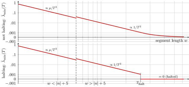
Figure 7: Lower bounds to the groundstate energy of the QTM history state Hamiltonian on a single segment, as a function of the segment length, in the halting and non-halting cases.

The top panel shows the case for which the dovetailed universal TM will not halt. Depending on the segment length $w$, we have the following two cases:

1. For $w<|\upeta|+5$, there is not enough tape for the phase expansion. By Lemma 16, we know that with probability $\geq\mu$, the phase estimation results in a string where the head symbol $q_{?}$ is over a tape qubit $\left\lvert{-}\right\rangle$, which shows the phase estimation truncated the output. Therefore, the head will be penalized by $\mathbf{P}$ with overlap $\geq\mu$. In order to account for the fact that the part of the computation following on from the garbage state coming out of the interrupted phase estimation could well halt, even if $\phi$ encodes a non-halting instance, we scale the lower bound in this area down by a factor $\mu$—which is still non-negative, as $\mu$ is just a constant prefactor. Observe that it is not essential that we inflict the penalty term at the end of the history state (see e.g. (Bausch et al., 2017, Cor. 44)).

2. For $w\geq|\upeta|+5$ the phase estimation finishes exactly, and the universal TM retrieves the complete input on which it will not halt; the energy penalty $\mathbf{P}$ applies as well.

In either case, the history state evolution is of length $T=T(w)$, i.e. the runtime of the computation until the head bumps into the right marker or the clock driving the computation runs out of time, both of which depends on the segment length $w$. In both cases, the last step of the computation will be completely penalized. This pushes the corresponding associated Hamiltonian’s ground state energy up by $\Theta(1/T^{2})$.

In case the dovetailed universal TM does halt, there is no further forward transition . The TM head will not feel the penalty $\mathbf{P}$, and the ground state energy is that of an unfrustrated history state Hamiltonian, i.e. zero. Observe that this happens at a point $T_{\mathrm{halt}}$ which is obviously independent from $w$. The precise statement is that once there is enough tape such that the entire evolution of the (halting) TM can be contained, no halting penalty will be felt. This happens once $w$ is such that $T(w)\geq T_{\mathrm{halt}}$. Define this segment length to be $w_{\mathrm{halt}}$.

After including the Marker Hamiltonian $\mathbf{H}_{s}^{(f)}$ in $\mathbf{H}_{s}$, we obtain the ground state energy bounds shown in Fig. 3. The dashed blue line shows an upper bound on the negative magnitude of the energy bonus $E(w)$ induced by the Marker Hamiltonian $\mu\mathbf{H}_{s}^{(f)}$ with $f(w)=2^{w}$. Note that we chose the loose bound $-\mu/T^{3+\delta}$ for visualization purposes. By Remark 12, we know that this bonus in fact satisfies $-\mu/2^{f(w)}\leq E(w)$. With Eq. 12, we know that

$$T^{3}(w) <2^{f(w)}\Longleftrightarrow\frac{1}{T^{3}(w)}>\frac{1}{2^{f(w)}}\geq-E(w),$$

and thus clearly

$$\operatorname{\lambda_{\mathrm{min}}}+E(w) \geq\bar{\lambda}_{\mathrm{min}}+E(w)>0.$$ (13)

Observe that $\mathbf{H}_{s}^{(f)}$ commutes with both $\mathbf{H}_{\mathrm{TM}}(\upeta)$ and $\mathbf{P}$, so the resulting ground state energy of $\mathbf{H}$ for the block of segment length $w$ will simply be

$$\operatorname{\lambda_{\mathrm{min}}}(\mathbf{H}_{s})=E(w)+\operatorname{\lambda_{\mathrm{min}}}(\mathbf{H}_{\mathrm{TM}}(\upeta)+\mathbf{P}).$$

The solid red line shows the lower bound achieved by subtracting the smaller attractive contribution $E(w)$ from the lower bound for $\operatorname{\lambda_{\mathrm{min}}}(\mathbf{H}_{\mathrm{TM}}(\upeta)+\mathbf{P})\geq\bar{\lambda}_{\mathrm{min}}$. We again consider each case separately.

If the dovetailed UTM does not halt, we subtract $|E(w)|$ (or, equivalently, add $E(w)$, since $E(w)$ is negative) from the lower bound we proved before. The ground state energy $\operatorname{\lambda_{\mathrm{min}}}+E(w)>0$ by Eq. 13.

If the UTM does halt, on the other hand, there exists a halting time $T_{\mathrm{halt}}$ such that $\bar{\lambda}_{\mathrm{min}}(w)=0$ for all $w>w_{\mathrm{halt}}$ (see magnified area). This immediately implies that

$$\operatorname{\lambda_{\mathrm{min}}}(w)\begin{cases}\geq\bar{\lambda}_{\mathrm{min}}(w)+E(w)>0&\text{for all $w<w_{\mathrm{halt}}$}\\ =-f(w)<0&\text{otherwise.}\end{cases}$$

This proves the last claim. ∎

We observe that in the halting case, the energy is smallest when the segment length is precisely $w_{\mathrm{halt}}$, as $|E(w)|$ is strictly monotonically decreasing.

In light of Remark 12, i.e. the fact that $\mathbf{H}^{(f)}$ breaks into signature blocks $\mathbf{H}^{(f)}_{s}$, we want to extend Theorem 20 to the case where the signature $s$ is not just a single segment, but a series of segments of varying length. We capture this in the following lemma.

Lemma 21.

Let the notation be as in Theorem 20, but take a signature $s$ with potentially multiple segment lengths $(w_{i})_{i}$ as in Theorem 11. Let $\nu(w_{i})$ be the energy of the ground state of a block segment of length $w_{i}$. Then

$$\operatorname{\lambda_{\mathrm{min}}}(\mathbf{H}_{s})=\sum_{i}\nu(w_{i}).$$

Proof.

Both $\mathbf{H}_{\mathrm{TM}}(\upeta)$ and $\mathbf{P}$ commute with $\mathbf{H}_{s}^{(f)}$, and we use the same Cartesian graph product argument for the latter as in Lemma 5. ∎

This leads us to the main technical theorem.

Theorem 22.

For any Turing machine $M$ and input $\upeta\in\mathds{N}$ to $M$, we can explicitly construct a sequence of 1D, translationally invariant, nearest-neighbour Hamiltonians $\mathbf{H}_{N}(\upeta,M)$ on the Hilbert space $(\mathds{C}^{d})^{\otimes N}$ with the property that either

1. $M(\upeta)$ does not halt, and $\operatorname{\lambda_{\mathrm{min}}}(\mathbf{H}_{N})\geq 0$ for all $N$, or

2. $M(\upeta)$ halts, and

   $$\operatorname{\lambda_{\mathrm{min}}}(\mathbf{H}_{N})\begin{cases}<-\lfloor N/w_{\mathrm{halt}}\rfloor\Omega(1/T_{\mathrm{halt}}^{3})&\text{$N>w_{\mathrm{halt}}$}\\ \geq 0&\text{$N\leq w_{\mathrm{halt}}$,}\end{cases}$$

   where $T_{\mathrm{halt}}$ is the time needed for $M(\upeta)$ to halt, and $w_{\mathrm{halt}}$ is the length of the tape accessed during the computation.

Proof.

We set $\mathbf{H}\coloneqq\mathbf{H}_{C}(M,\upeta)+\mathbf{H}^{(f)}$ for $\mathbf{H}_{C}(M,\upeta)=\mathbf{H}_{\mathrm{TM}}(M,\upeta)+\mathbf{P}$, and with $f(w)=w^{2}$ as in Lemma 21, but with the full Marker Hamiltonian $\mathbf{H}^{(f)}$ instead of a single signature block. We already know that $\mathbf{H}$ is block diagonal, and by Lemma 21 we know the spectrum of each block. There are two cases.

1. $M(\upeta)$ does not halt. By Theorem 20, we know that the ground state energy contribution of a single segment is falling off monotonically with the segment length. By Lemma 21, we know that the overall ground state energy is the sum of the individual segments. The block with the lowest energy is thus the one with a single segment of length $N$, and in particular non-negative (or if we do not penalize the rightmost halting boundary then the ground state energy is zero).

2. $M(\upeta)$ halts after $T_{\mathrm{halt}}$ steps, having consumed $w_{\mathrm{halt}}$ tape. If $N<w_{\mathrm{halt}}$ the same argument as above holds. If $N>w_{\mathrm{halt}}$, we have space for at least $\lfloor N/w_{\mathrm{halt}}\rfloor$ segments of tape on which the TM terminates. It is beneficial to have as many such segments as possible, as each of these contributes an energy $E(w_{\mathrm{halt}})<0$. Ignoring the right-most segment of non-full length (which is a single constant energy penalty), the block with a signature where the shortest possible segments on which the TM can halt are left-aligned has the lowest energy $<-\Omega(1/T^{3}_{\mathrm{halt}})$. Since there is only a single rightmost segment, but $O(N)$ bonus’ed segments, the asymptotic bound is $\operatorname{\lambda_{\mathrm{min}}}(\mathbf{H}_{N})<-\Omega(1/T_{\mathrm{halt}}^{3})$.

The claim follows. ∎

Note that the ground state energy of $\mathbf{H}$ diverges to minus infinity in the halting case, but the ground state energy density is bounded.

VII Undecidability of the Spectral Gap

In order to obtain the full result, we will need to shift the energy spectrum of $\mathbf{H}$ from Theorem 22 up so that its ground state is either $\geq 1$, or diverges towards $-\infty$, add a trivial Hamiltonian with ground state energy $0$, and another Hamiltonian with continuous spectrum. We begin by observing that an energy shift is readily achieved as follows.

Lemma 23.

By adding at most two-local identity terms, we can shift the energy of $\mathbf{H}$ from Theorem 22 such that

$$\operatorname{\lambda_{\mathrm{min}}}(\mathbf{H})\begin{cases}\geq 1&\text{if the TM does not halt,}\\ \longrightarrow-\infty&\text{in the halting case.}\end{cases}$$

Proof.

Employ Gottesman and Irani (2009)’s boundary trick again (cf. Remark 3), which hinges on the fact that there is $N$ one-local but only $N-1$ two-local terms. ∎

The next step is to construct a simple Hamiltonian with a unique ground state of energy $0$, and a spectral gap of $1$.

Lemma 24.

There exists a one-local translationally-invariant Hamiltonian $\mathbf{H}_{\mathrm{trivial}}$ on $(\mathds{C}^{2})^{\otimes N}$ which is diagonal in the computational basis, with unique zero-energy ground state $\left\lvert{00\cdots 0}\right\rangle$, and all other $\lambda\in\operatorname{spec}(\mathbf{H}_{\mathrm{trivial}})$ satisfy $\lambda\geq 1$.

Proof.

Take $\mathbf{H}_{\mathrm{trivial}}=\sum_{i=1}^{N}\left\lvert{1}\middle\rangle\!\middle\langle{1}\right\rvert_{i}$. ∎

Furthermore, we need a Hamiltonian with continuous spectrum in $[0,\infty)$ in the thermodynamic limit, which we call $\mathbf{H}_{\mathrm{dense}}$. With this, we can prove the following theorem.

Theorem 25.

Take $\mathbf{H}$ from Theorem 22 with shifted energy as in Lemma 23, and let $\mathcal{H}_{C}$ denote the Hilbert space on which it acts. Take $\mathbf{H}_{\mathrm{dense}}$ as defined and denote the Hilbert space on which it acts $\mathcal{H}_{\mathrm{dense}}$. Finally, let $\mathbf{H}_{\mathrm{trivial}}$ be the trivial ground-state-energy $0$ Hamiltonian from Lemma 24 with Hilbert space $\mathcal{H}_{\mathrm{trivial}}$. Then we can construct a Hamiltonian $\mathbf{H}_{\mathrm{tot}}=\mathbf{H}_{\mathrm{tot}}(\mathbf{H},\mathbf{H}_{\mathrm{dense}},\mathbf{H}_{\mathrm{trivial}})$ on $\mathcal{H}\coloneqq(\mathcal{H}_{C}\otimes\mathcal{H}_{\mathrm{dense}})\oplus\mathcal{H}_{\mathrm{trivial}}$ as in Section III.2 such that

$$\operatorname{spec}(\mathbf{H}_{\mathrm{tot}})=\{0\}\cup(\operatorname{spec}(\mathbf{H})+\operatorname{spec}(\mathbf{H}_{\mathrm{dense}}))\cup G,$$

where $G\subset[1,\infty)$.

Proof.

We use a trick from Bausch et al. (2018). Define

$$\mathbf{H}_{\mathrm{guard}}\coloneqq\sum_{i=1}^{N}(\mathds{1}_{1,2}^{(i)}\otimes\mathds{1}_{3}^{(i+1)}+\mathds{1}_{3}^{(i)}\otimes\mathds{1}_{1,2}^{(i+1)}).$$

It is clear that any state with support on both $\mathcal{H}_{C}\otimes\mathcal{H}_{\mathrm{dense}}$ and $\mathcal{H}_{\mathrm{trivial}}$ will incur an energy penalty from $\mathbf{H}_{\mathrm{guard}}$. Define further

$$\mathbf{H}_{\mathrm{tot}}=\mathbf{H}\otimes\mathds{1}_{2}\oplus 0_{3}+\mathds{1}_{1}\otimes\mathbf{H}_{\mathrm{dense}}\oplus 0_{3}+0_{1,2}\oplus\mathbf{H}_{\mathrm{trivial}}+\mathbf{H}_{\mathrm{guard}}.$$

Then the claim follows. ∎

Since the halting problem is undecidable in general, we obtain our main result Theorem 1, which we re-state in the following way.

Theorem 26 (Undecidability of the Spectral Gap in 1D).

Let $\beta\in(0,1]$ be arbitrary. Whether the Hamiltonian in Theorem 25 is gapped with a spectral gap of $1$, or is gapless, is undecidable, even if we multiply $\mathbf{H}$ and $\mathbf{H}_{\mathrm{dense}}$ by $\beta$. $\mathbf{H}_{\mathrm{tot}}$ can then be assumed to comprise local terms as laid out in Theorem 1.

Proof.

We note that the properties required from $\mathbf{H}$ and $\mathbf{H}_{\mathrm{dense}}$ in Theorem 25 remain true, independent of any constant prefactor $\beta$; i.e. the spectral gap for

$$\mathbf{H}_{\mathrm{tot}}= \ \beta(\mathbf{H}\otimes\mathds{1}_{2}\oplus 0_{3}+\mathds{1}_{1}\otimes\mathbf{H}_{\mathrm{dense}}\oplus 0_{3})$$

$$+ \ 0_{1,2}\oplus\mathbf{H}_{\mathrm{trivial}}+\mathbf{H}_{\mathrm{guard}}.$$

remains undecidable, for all $\beta>0$.

In addition, this means we can assume wlog that the local terms of $\mathbf{H}$ and $\mathbf{H}_{\mathrm{dense}}$ have norm $\|\cdot\|\leq 1$ for $\beta\leq 1$. The estimates of the norms in Theorem 1 then stem from computing the norms of the terms in $\mathbf{H}_{\mathrm{trivial}}$ and $\mathbf{H}_{\mathrm{guard}}$. ∎

VIII Extensions of the result

VIII.1 Periodic Boundary Conditions

Theorem 1 can, in a limited fashion, be extended to periodic boundary conditions, which we summarize in the following lemma and theorem.

Lemma 27.

Theorem 1 holds, even on 1D spin chains with periodic boundary conditions, and under the assumption that the spin chain instances all have length coprime to $P$, at the cost of a local dimension that grows with $P$.

Proof.

Take the Hamiltonian from Theorem 1. The only difference to the open boundary conditions case is that there is no mismatch between the number of 1- and 2-local terms, so we will have to modify those parts of the proof carefully.

We first note that Remark 3 relies on this boundary trick. In the periodic case, however, we cannot use it. The reason for Remark 3 was to enforce all segments to have right-boundaries—otherwise a segment which is half-unbounded on the right would pick up the bonus from the marker Hamiltonian, but no penalty due to the TM running out of tape. This problem never occurs on a ring: if there is at least one marker present, it is automatically guaranteed that each segment is properly bounded. Therefore, if we drop the term $\mathbf{P}^{\prime}$, Lemma 4 goes through, but such that the resulting Hamiltonian has a ground state energy of $0$, not $-4$.

The next step which needs amendment is in Theorem 10, where we note that there is no leftover penalty of $1/2$ from the leftmost boundary marker—bonus and penalty terms from Lemma 5 precisely cancel. To this end, there is no energy shift necessary.

The last issue is with Lemma 24: while one can straightforwardly create a Hamiltonian with constant negative ground state energy when there are open boundary conditions, this is not the case with periodic systems. To circumvent this, we assume we have a trivial Hamiltonian $\mathbf{H}_{\mathrm{trivial}}$ with unique classical ground state with energy 0 and first excited state 1. We then shift everything else up by a constant. Under the stated assumption that the spin loop has a length coprime to $P$, the positive energy shift can be achieved by adding an ancilliary Hilbert space of dimension $P$, and adding local projectors that enforce a tiling á la $1,2,3,\ldots,P$. Since this tiling has to be broken at least at one site on the ring, there is a constant energy shift.

The overall Hamiltonian then reads, as before,

$$\mathbf{H}_{\text{tot}}=\mathbf{H}^{\prime}\otimes\mathds{1}_{2}\oplus 0_{3}+\mathds{1}_{1}\otimes\mathbf{H}_{\mathrm{dense}}\oplus 0_{3}+0_{1,2}\oplus\mathbf{H}_{\mathrm{trivial}}+\mathbf{H}_{\mathrm{guard}}.$$

where $\mathbf{H}^{\prime}$ equals $\mathbf{H}$ from Theorem 1, with the $P$-periodic tiling enforced. In the non-halting case, $\mathbf{H}_{\text{tot}}$ will be gapped with $\Delta\geq 1$, and unique ground state. In the halting case, $\mathbf{H}^{\prime}$ will have an energy that diverges to $-\infty$ (despite the constant energy shift inflicted by the $P$-periodic tiling), and therefore pulls the dense spectrum of $\mathbf{H}_{\mathrm{dense}}$ with it. The claim of the theorem follows. ∎

VIII.2 Purely Transverse Field $\upeta$ Dependence

Thus far, the terms in Theorem 1 explicitly-dependent on the phase $\phi$ are two-local. More specifically, there are the one-local terms $\mathbf{a}^{\prime}$ with a coefficient of $\beta 2^{-2|\upeta|}$, as well as the terms $\mathbf{b}^{\prime\prime\prime}$ with prefactors $\exp(\pm\mathrm{i}\pi\phi(\upeta))$ and $\mathbf{b}^{\prime\prime\prime\prime}$ with prefactors $\exp(\pm\mathrm{i}\pi 2^{-2|\upeta|})$, respectively.

We can strengthen our findings by making the $\upeta$-dependent terms all one-local. This is a straightforward observation, and we will leave the details to the reader.

Remark 28.

There exists a variant of the QPE QTM such that the corresponding Hamiltonian $\mathbf{H}_{\mathrm{TM}}(\upeta)$ has only one-local terms that depend on $\upeta$.

Proof.

The two-local terms dependent on $\upeta$ stem from two steps of the phase estimation algorithm:

1. The controlled-phase gates with powers of the gate $\mathbf{U}_{\phi}$, and

2. the inverse QFT with powers of the controlled rotation $\mathbf{U}_{\alpha}$.

Naturally, any modification to the QPE QTM will directly translate to the corresponding history state Hamiltonian $\mathbf{H}_{\mathrm{TM}}$; in particular, if we manage to modify the algorithm to make the gates that depend on $\upeta$ one-local, the resulting Hamiltonian can be rendered one-local as well. To this end, we first note the circuit identity

@C=2em @!R=0em & 1
U        =       @C=2em @!R=0em & V 1 1
V V^†

where $\mathbf{V}=\sqrt{\mathbf{U}}$, as e.g. explained in (Nielsen and Chuang, 2010, fig. 4.6). Furthermore, we note that a generic translation of a circuit gate $\mathbf{V}$ to a Hamiltonian—say at time step $t$—results in a local term à la

$$\mathbf{h}_{\mathbf{V},t}=\sum_{i}\big{(}\left\lvert{t}\right\rangle\left\lvert{i}\right\rangle-\left\lvert{t+1}\right\rangle\mathbf{V}\left\lvert{i}\right\rangle\big{)}\big{(}\left\langle{t}\right\rvert\left\langle{i}\right\rvert-\left\langle{t+1}\right\rvert\left\langle{i}\right\rvert\mathbf{V}^{\dagger}\big{)}.$$

The locality of $\mathbf{h}_{\mathbf{V},t}$ thus crucially depends on how the clock is implemented, and there exists a long history of development rendering those transitions two-local Bausch et al. (2017); Gottesman and Irani (2009). Yet for our purposes we would like said gate to be implemented exactly, and such that if $\mathbf{V}$ depends on $\upeta$, the overall term does not become two-local. This can be achieved by ensuring that the clock transition $\left\lvert{t}\right\rangle\longmapsto\left\lvert{t+1}\right\rangle$ is a geometrically one-local term on the physical spins, during which $\mathbf{V}$ is applied to the quantum register contained within the very same spin. It is clear that this can be done in a translationally-invariant fashion within the context of Feynman’s standard circuit-to-Hamiltonian construction, at the cost of increasing the local dimension slightly. ∎

IX Discussion

In spite of indications that 1D spin chains are simpler systems than higher dimensional lattice models, we have shown that the spectral gap problem is undecidable even in dimension one, settling one of the big open questions left in Cubitt et al. (2015a). At the same time, the construction we present has some distinguishing features from the 2D construction.

In the 2D case, the ground state behaves as a highly non-classical model, showing all features of criticality, for any system size where the Universal Turing machine embedded in the model does not halt. If the machine eventually halts, starting from the corresponding system size the ground state will abruptly transition to a classical, product state. The construction we have presented shows the opposite property: the ground state is a product classical state of the trivial Hamiltonian $\sum_{i=1}^{N}\left\lvert{1}\middle\rangle\!\middle\langle{1}\right\rvert_{i}$ (i.e. $\left\lvert{00\cdots 0}\right\rangle$), unless the machine halts, in which case the low-energy spectrum of the Hamiltonian suddenly begins to converge to a dense set.

While both the 1D and 2D cases can be seen as an example of a size-driven phase transition Bausch et al. (2018), in the 1D construction we transition from trivial to gapless, instead of vice-versa. In 1D, there are algorithms with provably polynomial running time in the system size Landau et al. (2015). Nonetheless, our results prove that any numerical study of the ground-state properties will not reveal any of the phenomena one would expect of a gapless system. For both gapless and gapped cases, the numerics will instead find a classical ground state with constant gap above it, all the way up to some threshold chain length, which is uncomputable in general (determined by the tape length required for the universal Turing machine to halt, if it does indeed halt).

Therefore, not only is there no algorithm that can correctly predict whether a 1D Hamiltonian is gapped or not, but also the known efficient algorithms for computing ground state properties will fail to predict the correct thermodynamic properties of the state—even properties as elementary as the decay of correlations.

Of course the polynomial runtime of ground state approximation algorithms hinges on the promise that the one-dimensional system under study is asymptotically gapped, which is why we do not expect them to work e.g. for Hamiltonians with a QMA hard ground state problem. In fact, because of this, we know that all Hamiltonians of one-dimensional spin chains with a QMA hard ground state problem have to be gapless. Consequently, our 1D result implies that the premise itself on which all the efficient algorithms rely turns out to be undecidable.

Our findings extend to periodic boundary conditions, albeit in a limited fashion, for a number of spins promised to be coprime to some number $P$ (Section VIII.1). This comes at the cost of a local dimension that grows linearly with $P$. The general periodic case with fixed local dimension remains open. We further showed that the same result holds for the case where the $\upeta$-dependence is only on the one-local transverse field, and all two-local terms are fixed (Section VIII.2). As in 2D, the reduction also demonstrates that the ground state energy density of 1D spin chains is, in general, uncomputable.

An important question to ask is whether undecidability of the spectral gap is a generic feature, e.g. in the measure-theoretic sense over some underlying distribution, and whether the construction obeys some form of stability with respect to perturbations. The strongest-known stability proofs for general local perturbations only apply to certain types of frustration-free HamiltonianBravyi et al. (2010); Michalakis and Pytel (2013); Yarotsky (2006). Little is known about stability of the spectral gap to arbitrary local perturbations even for much simpler and far better–studied models than ours, such as the 1d transverse Ising model.

We can say a little more in our specific case. First, note that generic disordered local Hamiltonians—i.e. those where the local interaction terms are chosen uniformly at random, in particular not translationally invariant—are known to be gapless in 1D Movassagh (2017). This no longer holds true in the case of frustration-free translation invariant interactions Lemm (2019), while the question for generic translational invariant models is still open. Whether or not a random instance sampled from a collection of local terms is generically gapped or gapless thus depends on the choice of the underlying distribution. If, for instance, the local terms are those given in Theorem 1 (i.e. such that the phase gate for $\upeta$ and the encoded binary expansion length $|\upeta|$ match), and our choice of random distribution is over the encoded inputs $\upeta$—sampled with regards to some powerlaw distribution, say—then the probability that a random sample thereof has a decidable spectral gap depends on the universal Turing machine used within the construction. Yet in general even this probability itself can be uncomputable (cf. Chaitin’s constants Barmpalias and Dowe (2012)).

Similarly, the type of perturbation we allow determines whether we expect any type of robustness properties to hold. For instance, varying the classical couplings in Theorem 1 (e.g. $\mathbf{a}$ perturbed by a term $\epsilon\bar{\mathbf{a}}$ for small $\epsilon$) leaves the construction intact: any such term encoding a penalty or bonus diagonal in the computational basis will only change the corresponding energies by an amount $\propto\epsilon$. But bonus and penalty terms are of order one: for sufficiently-small $\epsilon$, the limiting behaviour of $\mathbf{H}_{N}$ remains unaltered. In contrast, the Feynman-Kitaev Hamiltonian terms are not robust to perturbations Bausch and Crosson (2018)—any such perturbation tends to produce a localized ground state which we expect to break the intended behaviour of our construction.

Perturbing the parameter $\upeta$ appearing in Eq. 3 will simply change the instance simulated by the UTM; yet for a generic such perturbation, the binary expansion $\phi(\upeta)$ is of course infinitely long. Since our construction cannot provide all those gates with bounded-norm local terms, this type of perturbation cannot be analysed within the scope of Hamiltonians we construct. On the other hand, perturbing the phase term $\phi(\upeta)$ such that its binary expansion remains bounded simply changes the encoded Turing machine input. This could, of course, change the behaviour between halting and non-halting. It is therefore intrinsic to this construction—and expected for any undecidable property of the Hamiltonian—that no form of stability should hold in the encoded phase.

An important point to emphasize is that, in the halting case, the critical behaviour exhibited by $\mathbf{H}_{N}$ depends on the behaviour of the dense spectrum Hamiltonian $\mathbf{H}_{\mathrm{dense}}$. As proven in Theorem 22, the ground state of $\mathbf{H}_{C}$ in the halting case is a product of segments of length just long enough for the encoded Turing machine to halt. While each segment can individually be uncomputably large (e.g. if the instance was a Busy Beaver) with a correspondingly uncomputable amount of entanglement entropy, the overall ground state remains product across these individual segments. This implies that even in the gapless phase, the entanglement entropy of the ground state of $\mathbf{H}_{C}$ is independent of the system size $N$, and only depends on the parameter $\upeta$.

Therefore, if the ground state of $\mathbf{H}_{\mathrm{dense}}$ has large entanglement entropy, so will have the ground state of $\mathbf{H}_{N}$, and thus detecting violation of entanglement entropy area laws is also undecidable. On the other hand there are instances of 1D Hamiltonians with dense spectrum whose ground states do not have large entanglement entropy Wolf et al. (2006); Fernández-González et al. (2014). Choosing such Hamiltonians in the construction will give a family of Hamiltonians $\mathbf{H}_{N}(M,\upeta)$ that always obeys an entanglement area law. Thus criticality is not essential to undecidability of the spectral gap; undecidability is possible even in cases where critical behaviour is guaranteed not to occur.

We conclude by mentioning an open question which is still to be addressed. As in the case of 2D systems, the model we present is extremely artificial, with a very large local dimension, which we did not try to optimize. It is an interesting problem whether it is possible to find more natural models exhibiting undecidable properties, or whether there is a local dimension threshold below which quantum systems necessarily behave in a predictable way Bravyi and Gosset (2015). I.e. does it hold that below some threshold on the local dimension the spectral gap problem becomes decidable? While size-driven phase transitions can happen in 2D with very small local dimension Bausch et al. (2018), these low-dimensional constructions are decidable. Determining if this threshold exists and if and how it depends on the lattice dimension remains a very interesting open question. The only known result in the other direction, proving decidability for frustration-free, nearest-neighbour qubit chains Bravyi and Gosset (2015), is also specific to 1D. Together with our 1D undecidability result, this gives strong evidence that the dimension threshold has a non-trivial answer.