Mining Contrasting Quasi-Clique Patterns

Abstract.

Mining dense quasi-cliques is a well-known clustering task with applications ranging from social networks over collaboration graphs to document analysis. Recent work has extended this task to multiple graphs; i.e. the goal is to find groups of vertices highly dense among multiple graphs. In this paper we argue that in a multi-graph scenario the sparsity is valuable for knowledge extraction as well. We introduce the concept of contrasting quasi-clique patterns: a collection of vertices highly dense in one graph but highly sparse (i.e. less connected) in a second graph. Thus, these patterns specifically highlight the difference/contrast between the considered graphs. Based on our novel model, we propose an algorithm that enables fast computation of contrasting patterns by exploiting intelligent traversal and pruning techniques. We showcase the potential of contrasting patterns on a variety of synthetic and real-world datasets.

1. Introduction

The World Wide Web, social networks, and e-commerce platforms have been successfully studied using various graph mining methods. One of most prominent tasks is mining quasi-cliques, i.e. detecting sets of vertices that are densely connected in a graph.

While traditionally only a single graph was considered, recent research (Pei et al., 2005; Wang et al., 2006; Zeng et al., 2006; Boden et al., 2012) has extended the search for quasi-cliques to the setting where multiple graphs are given (also known as multi-layer/multi-dimensional graphs). Often these graphs represent different types of connections (collaborations, similarity, citations, etc.). Here, the goal is to find groups of vertices that are densely connected among multiple graphs at the same time (cross-graph quasi-cliques); which has proven useful in several applications, most prominently in community detection (see e.g. (Kim and Lee, 2015)). While all existing work in the area of cross-graph quasi-cliques focused on detecting dense areas only, in this work we argue that for the multi-graph scenario sparsity is valuable as well.

Consider, for example, a graph of products in an e-commerce system where on one hand connections indicate co-purchases (graph 1), and on the other their textual similarity w.r.t their description (graph 2). Products highly connected in the co-purchasing graph but textually dissimilar are complementary products; e.g. socks and shoes are purchased together but have different description (see Fig. 1 for an illustrative example). In contrast, similar products not being purchased together are substitute products; e.g. the description of shoes is similar, but often only one model is purchased. Finding complementary and substitute products is useful to make meaningful product suggestions and improve the overall shopping experience (McAuley et al., 2015).

As another example, consider a graph of documents (e.g. scientific papers, websites, etc) where one graph (graph 1) represents citations between documents, and on the other their textual similarity (graph 2). Intuitively, a group of similar documents should be highly connected in the citation graph as well; e.g. papers about quasi-cliques are textually similar and often have a comparable state of the art. Thus, finding a group that is densely connected regarding their content, but sparsely connected regarding their citations is useful to detect, e.g., plagiarism or to identify missing connections between research works. We will show some real-world examples of these patterns in Sec. 5.2.

Figure 1. Contrasting quasi-clique pattern: The vertex set $\{B,C,D,E\}$ is dense in graph 1 (e.g. co-purchasing graph) but sparse in graph 2 (e.g. similarity graph).

Now, consider a group of people, one graph (graph 1) represents their day-to-day contact and the other (graph 2) their friendship on Facebook. People with whom we have a lot of interaction (e.g. friends or family) are expected to be Facebook contacts; i.e. dense in both graphs. However, people highly connected in the Facebook graph and at the same time sparsely connected in the contact graph is an interesting pattern to give insights for a social or psychological study, while people highly connected in the contact graph with few connections in the Facebook graph might represent a different type of relationship; e.g. in principle, teachers, bosses, and supervisors are not expected to be Facebook friends. Later in Sec. 5.2 we show a real case study showing interactions between High School students as given by (Mastrandrea et al., 2015).

As these examples indicate, in a multi-graph scenario sparsity becomes an important characteristic. Based on this motivation, this paper introduces the concept of contrasting quasi-clique patterns (CQC patterns): a collection of vertices highly dense in one graph, and simultaneously sparse in a second graph.

In our model, we consider the fact that a vertex can naturally belong to more than one pattern. Thus, we allow our patterns to overlap. However, allowing overlap often leads to the problem of redundancy since many similar patterns might be generated (Müller et al., 2009; Günnemann et al., 2010). Thus, based on our novel pattern definition, we introduce a model for generating a set of patterns that are non-redundant, though, still allows the patterns to overlap to a certain extend. This final set of patterns should contain the most contrasting patterns.

Finally, since determining the overall clustering according to our model is NP-hard, we introduce an approximate algorithm to compute it. The idea is to use a best-first principle to explore a joint enumeration tree in an informed fashion; thus, analyzing both graphs simultaneously and starting to enumerate the most contrasting patterns first. Our experimental analysis shows that this specialized approach is much more efficient than relying on existing dense cross-graph quasi-clique detection methods.

The contributions of this work are as follows:

• We introduce the problem of finding contrasting quasi-cliques patterns (CQC patterns).

• We propose the algorithm MiSPa to approximate the problem of finding CQC patterns.

• We perform experiments on several real-world datasets confirming the potential of our novel pattern definition.

We want to highlight that our task is different to discriminative subgraph discovery and to community detection in signed networks (see. Sec. 2).

Overview. Sec. 2 presents related work. Sec. 3 introduces the CQC pattern model, followed by our MiSPa algorithm in Sec. 4. Sec. 5 shows our experiments, and Sec. 6 concludes the paper.

2. Related Work

Multiple mining tasks for graphs exist (Aggarwal and Wang, 2010). Relevant to this work is the field of “dense subgraph mining”. Here, different models and notions have been introduced, with cliques and $\gamma$-quasi-cliques (Pei et al., 2005; Liu and Wong, 2008) being the most prominent ones.

Several clustering approaches have been proposed which take a set of networks as input, where each network represents a particular kind of relationship. This type of data if often called multi-relational network (Cai et al., 2005). The work (Cerf et al., 2009b), for example, aims to find cliques in subsequent time steps in a dynamic graph represented as a 3-dimensional boolean cube. By basing on the algorithm of (Cerf et al., 2009a), the desired cliques are specified by (anti-)monotonic constraints. Since it exploits the (anti-)monotonic property of cliques, an extension to quasi-cliques is not possible as the quasi-clique model does not fulfill a monotonicity property.

In (Pei et al., 2005), the principle of cross-graph quasi-cliques detection has been introduced. Given a database of graphs each having the same vertices, a cross-graph quasi-clique is defined as a set of vertices that forms a quasi-clique in all of the graphs. Only maximal sets having this property are output. Similarly, the approaches (Wang et al., 2006) and (Zeng et al., 2006) mine sets of vertices that form a clique (Wang et al., 2006) or quasi-clique (Zeng et al., 2006) in at least a certain percentage of the graphs in the database. Both approaches aim at mining closed (quasi-)cliques. Last, in (Boden et al., 2012) a method for finding non-redundant quasi-cliques spanning across multiple graphs has been proposed.

All of the above works focused on finding dense quasi-cliques only. In contrast, our work aims at finding contrasting patterns: groups of vertices that are dense and sparse at the same time.

As a naive approach to detect contrasting patterns one could consider to use one of the above dense subgraph mining algorithms when operating on the complement graphs. We compare with such an approach in our experimental study.

Finally, please note that the task of community detection in signed networks (Anchuri and Magdon-Ismail, 2012; Esmailian and Jalili, 2015), i.e. networks with positive and negative edges, is different to our principle. There, one is still interested in finding dense clusters, with edges of different kind. Negative edges, however, do not mean sparsity – which is the focus of this work. Indeed, signed networks and our principle could be combined.

Also note the difference to the principle of discriminative subgraph mining (Thoma et al., 2010; Jin and Wang, 2011; Ting and Bailey, 2006) (rarely also called contrast subgraphs as in (Ting and Bailey, 2006)), a supervised-learning task. Here a database of multiple (usually attributed) graphs is given, each belonging to a certain class we aim to predict. The goal is to find subgraphs that discriminate between the classes, i.e. subgraphs appearing in many graphs of one class but only few graphs of the other classes. Whether these subgraphs are dense or sparse is not relevant.

3. Pattern Model

This section formalizes the problem of finding contrasting quasi-clique patterns (CQC patterns); a collection of vertices dense in one graph but sparsely connected in the other. To this aim we appeal to the notion of quasi-cliques, a set of vertices which is almost completely connected.

There have been multiple works on quasi-cliques which rely primarily on two formulations. We will show that choosing a single quasi-clique formulation to detect CQC patterns has severe drawbacks. Thus, we combine both definitions in a single measure of interestingness.

The input under consideration is a set of graphs $\mathcal{G}=\{G_{1},G_{2}\}$ where each graph $G_{i}=(V,E_{i}),E_{i}\subseteq V\times V$ is an undirected graph without self-loops. Both graphs share the same vertices but with different edges. Note that it is possible to consider different vertex sets $\{V_{1},V_{2}\}$ by simply using $V=\bigcup V_{i}$.

3.1. Existing quasi-clique models and their limitations to detect CQC patterns

Before specifying our new model, we first introduce the existing quasi-clique models and highlight their limitations for CQC patterns detection. The first definition of quasi-cliques as, e.g., given by (Boden et al., 2012; Liu and Wong, 2008; Zeng et al., 2006) is:

Definition 3.1 ($\delta$-Quasi-clique).

Given a vertex set $O\subseteq V$ in a graph $G_{i}=(V,E_{i})$, and $\delta\in(0,1]$, $O$ is a $\delta$-quasi-clique if

$$\forall v\in O:deg^{O}_{G_{i}}(v)\geq\lceil\delta\cdot(|O|-1)\rceil$$

where $deg^{O}_{G_{i}}(v)=|\{u\in O\mid(u,v)\in E_{i}\}|$. The density of a quasi-clique $O$ in graph $G_{i}$ is defined by

$$\textstyle\gamma_{G_{i}}(O)=\frac{\min_{v\in O}\{deg^{O}_{G_{i}}(v)\}}{|O|-1}$$

The higher $\delta$, the higher the required density of the quasi-clique. For $\delta=1$, the definition represents cliques.

The second definition of quasi-cliques, inspired by works like (Uno, 2010; Moser et al., 2009), is defined as follows:

Definition 3.2 ($\theta$-Quasi-clique).

Given a connected vertex set $O\subseteq V$ in a graph $G_{i}=(V,E_{i})$, and $\theta\in(0,1]$, $O$ is a $\theta$-quasi-clique if

$$\alpha_{G_{i}}(O)\geq\theta$$

where $\alpha_{G_{i}}(O)=2|E_{i}(O)|/(|O|\cdot(|O|-1))$ is the proportion of observed edges $E_{i}(O)$ in $O$ w.r.t graph $G_{i}$ compared to the potential edges in a (complete) clique, called simply density.

The crucial difference between both definitions is that in a $\delta$-quasi-clique each vertex has to be sufficiently connected, while in a $\theta$-quasi-clique only the average density is important. This seemingly small difference has a severe effect when trying to find dense or sparse regions in a graph.

1) When considering dense regions, the $\delta$-quasi-clique definition favors the desirable detection of “tightly and relatively evenly” connected quasi-cliques as shown by (Zeng et al., 2006) – i.e. the density is relatively homogeneous in the pattern. In graph 2 of Figure 2, the set $O=\{A,B,C,D\}$ is a valid $\delta$-quasi-clique, while the set $O^{\prime}=\{A,B,C,D,E\}$ is none. This property matches the intuition, since the node $E$ has only one edge, making the pattern unevenly connected and not helpful for the density of the group.

In contrast, using $\theta$-quasi-clique the set $O^{\prime}$ would still be regarded as relatively dense ($\alpha=7/10$). Thus, $\delta$-quasi-cliques are better suited for finding homogeneous dense regions.

2) When considering sparse regions, the roles switch: Since the definition of $\delta$-quasi-cliques enforces each vertex to be sufficiently connected, a single less-connected vertex would lower the density significantly. In Figure 2, the density of the vertex set $O^{\prime}=\{A,B,C,D,E\}$ in graph 2 is $\gamma=0.25$, i.e. seemingly sparse – while obviously the region is not entirely sparse. By contrast, the $\theta$-quasi-clique definition does not suffer from this drawback.

While clearly each definition of density and sparsity has its own characteristics, we argue that the resulting patterns should be relatively homogeneous regarding their density and sparsity. That is, the density/sparsity should not just be the effect of individual nodes.

Accordingly, since our goal is to find highly dense vertices in one graph which are sparsely connected in the other, we combine the rationale behind $\delta$ and $\theta$ quasi-cliques. While $\delta$ is more suited to capture density, $\theta$ is better to capture less connected vertices.

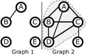
Figure 2. Example to illustrate our CQC pattern model

3.2. CQC patterns

More precise: First, we ensure that the nodes in one graph are sufficiently connected using the $\delta$-quasi-clique model. Second, to define sparsity – or more precise our measure of contrast – we borrow from the $\theta$-quasi-clique definition by referring to the density measure $\alpha$; i.e. the fraction of observed edges compared to the potential edges: If the fraction is high in one graph but low in the other, we observe a significant difference in the number of edges. Thus, the contrast of their density values is high.

Formally:

Definition 3.3 ($(\delta,\delta^{\prime})$-contrasting quasi-clique).

Given a vertex set $O\subseteq V$, graphs $\mathcal{G}=\{G_{1},G_{2}\}$, $\delta\in(0,1]$, and $\delta^{\prime}\in(0,1]$. $O$ is a $(\delta,\delta^{\prime})$-CQC pattern if

• $\max\{{\gamma}_{G_{1}}(O),{\gamma}_{G_{2}}(O)\}\geq\delta$   // i.e. $O$ is a $\delta$-quasi-clique in at least one graph

• $c(O)>\delta^{\prime}$   // i.e. the contrast in densities is high

where $c(O):=|\alpha_{G_{1}}(O)-\alpha_{G_{2}}(O)|$ is the contrast of the pattern.

To illustrate better CQC patterns consider Fig 2, and the set $O=\{A,B,C,D\}$. In the second graph, $O$ is a quasi-clique of high density ($\gamma=1$); in contrast, in the first graph, the density is zero since $C$ and $D$ are disconnected. The contrast value is given by $6/6-1/6=(6-1)/(0.5\cdot 4\cdot 3)=0.83$. Thus, $O$ is a $(1,0.83)$-CQC pattern. The set $O^{\prime}=\{A,B,C,D,E\}$ is not a CQC pattern; $O^{\prime}$ is not a $\delta$ quasi-clique in any of the graphs.

3.3. Selection of $\delta$ and $\delta^{\prime}$

The CQC patterns can be controlled by selecting $\delta$ and $\delta^{\prime}$. A low value of $\delta$ produces sparse patterns while a large value dense ones. Also, if we set $\delta^{\prime}$ to a large value we get patterns with more difference in the number of edges – or more precise a high contrast – while a small $\delta^{\prime}$ favors the detection of patterns with few contrast. Thus, by combining both parameters into a single definition (i.e. CQC patterns), we should consider the influence that both have in the final result. As an example, a small $\delta$ and a large $\delta^{\prime}$ (i.e. sparse vertices with high contrast) might produce no patterns at all wasting computational resources. By contrast, if we set $\delta$ to a large value and $\delta^{\prime}$ to a small one we get highly dense patterns with contrast.

Further, notice that a CQC pattern pattern has to be, first, a potential quasi-clique in at least one of the graphs before considering it a contrasting pattern. Thus, $\delta$ heavily influences the number of potential patterns to investigate while $\delta^{\prime}$ refines the enumeration of these by means of an upper bound on the interestingness of the patterns as we shall show below (in Section 4.4).

In general, we suggest to fix $\delta^{\prime}=0$ (i.e. we will be interested in all patterns with contrast) and set $\delta\geq 0.5$, since in this case the nodes are tightly connected and guaranteed to be connected (Zeng et al., 2006).

3.4. Overall pattern result

Multiple sets of vertices can fulfill the definition of CQC patterns, thus, potentially leading to a large amount of patterns that are quite similar – and, therefore, not interesting for the user. In Fig. 3, e.g., the set $O=\{A,B,C,D\}$ and $P=\{A,C,D\}$ are both reasonable CQC patterns; however, they capture almost the same information.

Figure 3. Example to illustrate redundant CQC patterns

To refine the output to a smaller subsets of patterns, we consider only the most interesting, non-redundant ones.

What are the interesting patterns? We argue that two aspects are of primary importance for our task: First, patterns showing a high contrast are interesting. Observing a set of vertices that is completely connected in one but completely unconnected in the other graph is a surprising result. Second, patterns of large size are interesting. This matches the idea of classical quasi-clique approaches where primarily maximal patterns are detected. We here simply combine both measures into a single interestingness function

(1) $$\textstyle I(O):=|O|\cdot c(O)=\frac{2\cdot\text{abs}(|E_{1}(O)|-|E_{2}(O)|)}{|O|-1}$$

Furthermore, patterns which are not 0.5 quasi-cliques in at least one of the graphs and which are smaller than 4 vertices are not interesting; i.e. we set $I(O)=-1$ for these patterns.

What are redundant patterns? To define redundancy, we adapted the redundancy relation as described in (Boden et al., 2012). Intuitively, a pattern $O$ is redundant to a pattern $P$, if it is less interesting and a high fraction of $O$’s edges are already covered by $P$. Formally,

Definition 3.4 (Redundancy).

Let $O$ and $P$ be two CQC patterns. $O$ is redundant to $P$ (short: $O\prec P$) if

$$O\neq P\wedge I(O)\leq I(P)\wedge\frac{1}{2}\sum_{i\in\{1,2\}}\frac{|E_{i}(O)\cap E_{i}(P)|}{|E_{i}(O)|}\geq r$$

for the redundancy parameter $r\in(0,1]$.

Consider again Fig. 3: The set $O=\{A,B,C,D\}$ has an interestingness of $I(O)=4\cdot 0.5=2$, the set $P=\{A,C,D\}$ of $I(P)=3\cdot 1=3$, and the set $Q=\{B,D,E,F\}$ of $I(Q)=4\cdot 0.66=2.66$. In this example $P$ is more interesting than $O$ since $P$ is not connected at all in the second graph. Thus, $O$ is redundant to $P$ since it is less interesting and they share most of their edges. $Q$ is not redundant to the other patterns since it covers different edges.

Given the interestingness function and the redundancy relation, we define the final output as the result of a constrained combinatorial optimization problem. We aim to find a set of CQC patterns that are pairwise non-redundant and together maximize the interestingness. Formally,

Definition 3.5.

The final result of patterns is given by

$$\mathcal{R}^{*}=\arg\max_{\stackrel{{\scriptstyle\mathcal{R}\subseteq\mathcal{D}}}{{\neg\exists O,O^{\prime}\in\mathcal{R}:O\prec O^{\prime}}}}\Sigma_{O\in\mathcal{R}}I(O)$$

where $\mathcal{D}:=\{O\subseteq V\mid O\text{ is a $(\delta,\delta^{\prime})$-CQC pattern and $I(O)>0$}\}$ is the set of all interesting CQC patterns

3.5. Complexity of Finding CQC patterns

The problem of finding CQC patterns is NP-hard. This can be shown by reducing the NP-hard quasi-clique detection problem (Liu and Wong, 2008) to our problem: Assume we want to find (or even enumerate) quasi-cliques in a graph $G=G_{1}$. By constructing a second graph $G_{2}$ without any edges, the detection of $(\gamma,0)$-contrasting quasi-cliques in $\{G_{1},G_{2}\}$ corresponds to finding $\gamma$-quasi-cliques in $G_{1}$. Hence, our problem is NP-hard, and requires an approximate solution for efficiency.

4. Algorithm MiSPa

To compute CQC patterns one approach is to use an efficient algorithm to find quasi-cliques (e.g. (Boden et al., 2012; Moser et al., 2009; Zeng et al., 2006; Liu and Wong, 2008)) in each individual graph first. Then for each cluster one can compute the density of the clusters with respect to the other graph to check whether a high contrast is obtained. Finally, the most interesting and non-redundant patterns can be selected in a post-processing step.

This approach has two severe limitations: First, one might generate a large set of uninteresting patterns that are dense in both graphs. Thus, only wasting computation time. On the other hand, one might miss important patterns. Since the existing quasi-clique approaches are steered towards finding dense subgraphs only, slightly less dense subgraphs might not be reported – these subgraphs, however, might show much stronger contrast values regarding the second graph.

Hence, we have designed the MiSPa algorithm to efficiently identify CQC patterns. Our algorithm is inspired by the MiMAG algorithm (Boden et al., 2012) that simultaneously analyzes multiple graphs. The huge difference being that our algorithm is steered towards finding high contrast patterns.

Based on Sec. 3.5, we cannot expect to find an efficient algorithm computing an exact result. Thus, instead of determining a result with maximum interestingness, we compute a maximal result. That is, a result where patterns are pairwise non-redundant, have high interestingness, and adding any further pattern would lead to redundancy.

The core idea we follow is twofold: (i) instead of analyzing the graphs individually, we traverse them jointly, and (ii) we traverse the graphs in a informed fashion to enumerate the most interesting patterns first. For this purpose, we adapt the traversal principle proposed in (Liu and Wong, 2008; Boden et al., 2012).

4.1. Joint enumeration tree

In our algorithm, vertex sets $O\subseteq V$ are enumerated by a traversal in the set enumeration tree (Rymon, 1992). An example tree for a graph with three vertices is shown in Figure 4. Basically, the set enumeration tree contains all possible vertex sets $O\subseteq V$. Each set visited by the traversal of the tree is a potential CQC pattern.

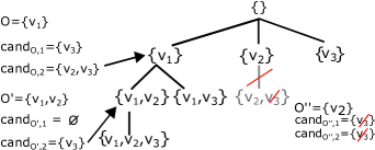
Figure 4. Joint set enumeration tree

The crucial aspect is to prune this enumeration tree, i.e. to avoid traversing it completely. For this purpose, each node $O$ is associated with two candidate sets $cand_{O,1}$ and $cand_{O,2}$. The candidate set $cand_{O,i}$ contains all vertices that can (potentially) be added to $O$ to form a quasi-clique in graph $i$ (one property of our CQC patterns definition). Note that these two candidate sets might (and will primarily) be different since our goal is to find patterns $X\supseteq O$ that are dense in one graph but sparse in the other.

To lower the cardinality of a candidate set, we apply multiple pruning methods (Liu and Wong, 2008). That is, if $O$’s candidate set $cand_{O,i}$ contains a vertex $v$ that can never be part of a quasi-clique $O^{\prime}\supset O$ in graph $i$, we can delete $v$ from the candidate set. If a vertex $v$ can be removed from both candidate sets, the whole subtree rooted at the current node that contains $v$ can be pruned. In none of the graphs, the vertex can be part of a quasi-clique $X\supseteq O\cup\{v\}$. As an example, consider Figure 4 and assume $v_{3}$ is not a promising vertex w.r.t the node $O^{\prime\prime}=\{v_{2}\}$, then $v_{3}$ can be deleted from both $cand_{O^{\prime\prime},1}$ and $cand_{O^{\prime\prime},2}$. Lastly, since both candidate sets are empty, the subtree rooted at $\{v_{2}\}$ can be safely pruned as it can never be part of a quasi-clique.

4.2. Informed tree traversal

The above pruning principle lowers the area of the search space that needs to be investigated. However, still too many patterns might be required to analyze. Therefore, in a next step, instead of following an uninformed (e.g. depth-first) traversal of the tree as in (Liu and Wong, 2008), we perform a best-first (A*-like) traversal.

To realize this informed search, we need to provide bounds / estimates for the interestingness of the patterns expected in a subtree. For each node $O$, we compute a estimation that provides an upper bound for the maximal interestingness of any pattern that can be found in the subtree rooted at $O$. Using this bound, we traverse the most promising subtrees first. In Section 4.4, we show how to compute this bound.

Given this informed search, for each set $O$ we visit during the traversal, we check if $O$ forms a valid CQC pattern. If so, we add it to an intermediate priority queue – we cannot add it to the final result yet since there might be further more interesting patterns in other subtrees (the estimated interestingness provides an upper bound of the subtree’s interestingness only; thus, $O$ itself might have a lower interestingness). This priority queue contains the set of subtrees that are still to process, as well as the set of already detected patterns that are not added to the result so far. This queue is sorted by the (estimated) interestingness values of the subtrees and patterns.

4.3. Overall Processing Scheme

Based on these ideas, the overall processing of MiSPa is shown in Algorithm 1. Given the two input graphs, MiSPa computes a maximal set of CQC patterns which contains only non-redundant patterns. Initially, the set $Result$ is empty (line 3); it will be iteratively filled during the processing. The priority queue contains initially one element which represents the root node of the joint set enumeration tree (line 4) – at the root, the traversal has to start. Then this queue is processed until it is empty.

If the first element of the queue is a CQC pattern, no better patterns can exist; in this case (and if the pattern is non-redundant to previously selected patterns), we can add it to the result set (line 8). In contrast, if the first element is a subtree, we continue with the best-first travel.

In detail, ’continuing the traversal’ means: Given the current subtree – e.g. rooted at $O$ –, we first pick one of the vertices $u\in\bigcup_{i\in\{1,2\}}cand_{O,i}$ from $O$’s candidate set. Here, we use the vertex having the highest degree w.r.t. $O$ since it most probably leads to dense subgraphs. We then check whether $O\cup\{u\}$ is a valid CQC pattern; if so, we add it to the queue. Besides the pattern, two further objects are added to the queue: the new subtree rooted at $O\cup\{u\}$, and the subtree still rooted at $O$ – but now removed by the branch which represents the already added $O\cup\{u\}$. For example, in Fig. 4, assuming we are inspecting the subtree rooted at $\{v_{1}\}$, one would add the subtree rooted at $\{v_{1},v_{2}\}$ as well as the subtree $\{v_{1}\}$ removed by the branch $\{v_{1},v_{2}\}$ to the queue.

In general, by always adding these two subtrees to the queue, we ensure that each node in the joint set enumeration tree is exactly visited once. Simultaneously, the overall priority queue ensures that subtrees and patterns with a high interestingness are processed first: The queue is sorted by the (actual/estimated) interestingness values of the patterns/subtrees. Even more, since the estimated interestingness values of the subtrees are upper bounds on the actual interestingness of the contained patterns, this processing guarantees that patterns are added to the final result in monotonically decreasing order of their interestingness values – thus, approximating our goal of Definition 3.5.

Algorithm 1 MiSPa: Best-first search for CQC patterns

1:Graphs $G_{1},G_{2}$ with $G_{i}=(V,E_{i})$

2:Maximal set $Result$ of non-redundant patterns

3:$Result:=\emptyset$ $\triangleright$ Final result set

4:$queue:=[~{}(\emptyset,[cand_{\emptyset,i}=V]_{i\in\{1,2\}})~{}]$ $\triangleright$ Priority queue of patterns & subtrees

5:while $queue$ not empty do

6:   $Obj:=queue.\mathrm{pop}()$ $\triangleright$ Select object with highest interestingness

7:   if $Obj$ is a CQC pattern $O$ then

8:     if $\neg\exists P\in Result:O\prec P\vee P\prec O$ then $Result.add(O)$      

9:   else$\triangleright$ $Obj$ is subtree $ST=(O,[cand_{O,i}]_{i\in\{1,2\}})$

10:     continue tree traversal at $ST$

11:     $\triangleright$ thus adding potential patterns and child-subtrees to the queue    

12:return Result

Theorem 4.1.

Algo. 1 generates a maximal set of non-redundant CQC patterns.

Proof.

(Sketch) (i) Clearly the result contains no redundancy as ensured by line 8. (ii) The tree traversal ensures that every node which might be a CQC pattern is visited. Further, every node that is a CQC pattern, will be added to the queue. Since the queue is processed until empty, every pattern is either redundant or added to the result. Thus, the result is maximal. ∎

Computational Complexity: MiSPa follows an A*-like principle to enumerate contrasting patterns. Thus, its efficiency depends on the bounds for the interestingness of subtrees; we shall show below in Sec. 4.4 how we determine this upper bound. In the worst case, each node in the enumeration tree has to be visited leading to an exponential complexity in the number of vertices, as in the A*-search strategy. However, in practice our upper bounds combined with our pruning strategies result in fewer nodes visited in the enumeration tree. Indeed, in Sec. 5.3, we study an alternative to MiSPa by turning off all these techniques demonstrating the effectiveness of our pruning strategy in real-world datasets.

4.4. Bounds for the Interestingness

Last, we present our upper bound for the interestingness of subtrees. This bound is crucial for the best-first traversal and to find the most interesting patterns. Moreover, if the estimate is not positive we can even prune the whole subtree since no interesting patterns can be found in it.

Formally, we are interested in finding a function $I^{*}(O)$ such that

$$\text{ $\forall X\supset O,X\subseteq S_{O}$: $X$ is a CQC pattern}\Rightarrow I(X)\leq I^{*}(O)$$

where $S_{O}:=O\cup cand_{O,1}\cup cand_{O,2}$. That is, the interestingness of each CQC pattern located in the subtree rooted at $O$ is bounded from above by $I^{*}(O)$. Of course, the bound needs to be efficiently computable, i.e we cannot simply enumerate all $X$.

To derive the bound, let us first introduce a definition. The set of edges connecting two disjoint sets $A$ and $B$ in graph $i$ is denoted with

$$E_{i}(A\leftrightarrow B):=\{(u,v)\in E_{i}\mid u\in A,v\in B\}$$

Thus, $|E_{i}(A\leftrightarrow B)|=\sum_{a\in A}deg_{G_{i}}^{B}(a)=\sum_{b\in B}deg_{G_{i}}^{A}(b)$ where $deg_{G_{i}}^{Y}(x)$ (see. Def. 3.1) denotes the degree of vertex $x$ w.r.t. the set $Y$ in graph $i$.

Since the interestingness (Eq. (1)) decomposes into the difference in the number of edges and the cardinality of the set, we first derive the following result:

Theorem 4.2.

Assume $X$, $O\subset X\subseteq S_{O}$, is a CQC pattern which forms a quasi-clique in graph $i$, it holds: $|E_{i}(X)|-|E_{j}(X)|\leq d_{ij}(O)$ where

(2) $$\begin{split}d_{ij}(O):=|E_{i}(O)|-|E_{j}(O)|+\!\!\!\!\!\!\!\!\!\sum_{v\in cand_{O,i}}\!\!\!\!\max\{0,deg_{G_{i}}^{O}(v)-\\ deg_{G_{j}}^{O}(v)+\frac{1}{2}deg_{G_{i}}^{cand_{O,i}}(v)\}\end{split}$$

Proof.

Clearly $E_{i}(X)=E_{i}(O)\cup E_{i}(X\backslash O)\cup E_{i}(O\leftrightarrow X\backslash O)$. And since the above sets are disjoint $|E_{i}(X)|=|E_{i}(O)|+|E_{i}(X\backslash O)|+|E_{i}(O\leftrightarrow X\backslash O)|$. Further, since we consider undirected graphs we have $|E_{i}(X\backslash O)|=\frac{1}{2}\sum_{v\in X\backslash O}deg_{G_{i}}^{X\backslash O}(v)$. And since $X$ is assumed to be a quasi-clique in graph $i$ (i.e. $X\subseteq O\cup cand_{O,i}$), we have $deg_{G_{i}}^{X\backslash O}(v)\leq deg_{G_{i}}^{cand_{O,i}}(v)$. It follows, $|E_{i}(X)|-|E_{j}(X)|=|E_{i}(O)|-|E_{j}(O)|+|E_{i}(O\leftrightarrow X\backslash O)|-|E_{j}(O\leftrightarrow X\backslash O)|+E_{i}(X\backslash O)|-E_{j}(X\backslash O)|\leq|E_{i}(O)|-|E_{j}(O)|+\sum_{v\in X\backslash O}[deg_{G_{i}}^{O}(v)-deg_{G_{j}}^{O}(v)+\frac{1}{2}deg_{G_{i}}^{X\backslash O}(v)]\leq|E_{i}(O)|-|E_{j}(O)|+\sum_{v\in X\backslash O}\max\{0,deg_{G_{i}}^{O}(v)-deg_{G_{j}}^{O}(v)+\frac{1}{2}deg_{G_{i}}^{cand_{O,i}}(v)\}\leq|E_{i}(O)|-|E_{j}(O)|+\sum_{v\in cand_{O,i}}\max\{0,$ $deg_{G_{i}}^{O}(v)-deg_{G_{j}}^{O}(v)+\frac{1}{2}deg_{G_{i}}^{cand_{O,i}}(v)\}$ ∎

The above result gives an estimate on the edge difference in a CQC pattern. Note that it is highly efficient to compute since we only have to iterate once through all vertices in the candidate set $cand_{O,i}$. The number of edges in $O$ as well as the degrees can easily be maintained during the run of the algorithm and don’t need to be recomputed all the time. Using the above result leads to:

Theorem 4.3.

Assume $X$, $O\subset X\subseteq S_{O}$, is a CQC pattern, it holds: $I(X)\leq I^{*}(O):=\frac{2}{|O|}\max\{d_{12}(O),d_{21}(O)\}$

Proof.

$I(X)=\frac{2\cdot\text{abs}(|E_{1}(X)|-|E_{2}(X)|)}{|X|-1}\leq$ $\frac{2\cdot\text{abs}(|E_{1}(X)|-|E_{2}(X)|)}{|O|}\leq\frac{2\cdot\max\{d_{12}(O),d_{21}(O)\}}{|O|}$ ∎

Given that $I(X)\leq I^{*}(O)$, we can safely prune the whole subtree when $I^{*}(O)\leq 0$ since there is no contrast at all.

5. Experimental Evaluation

In the following, we evaluate the quality of the detected patterns and runtime of our algorithm on synthetic and real-world datasets. As there is no ground-truth available regarding contrasting patterns, which hinders the evaluation of the algorithm, we highlight some characteristics of the resulting contrasting patterns.

Parameter selection. The redundancy parameter $r$ along with $\delta$ and $\delta^{\prime}$ play a relevant role in the task of mining contrasting patterns. To showcase our CQC pattern model and the MiSPa algorithm, in our experimental setting, we have used $\delta\geq 0.5$ and $\delta^{\prime}=0$; i.e. we are interested in any contrasting pattern that is tightly and evenly connected in at least one graph (see Sec. 3). Also, we have set $r=0.1$ as our interest is in patterns with low redundancy.

Still, we believe that these parameters should be selected according to the application of interest. Thus, our algorithm and all used datasets are available at URL.

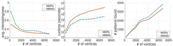
Figure 5. Quality, runtime, and number of patterns of MiSPa contrasted against MiMAG.

Competing approaches. Intuitively, to detect contrasting patterns, it would be possible to consider the complement graphs and apply a dense subgraph extraction algorithm on them. That is, given two graphs $G_{1}=(V,E_{1})$ and $G_{2}=(V,E_{2})$ build their complements $\overline{G_{1}}=(V,\overline{E_{1}})$, $\overline{G_{2}}=(V,\overline{E_{2}})$ where $\overline{E_{i}}=(V\times V)\setminus E_{i}$. Then, apply a cross-graph quasi-clique method first on the combination $G_{1},\overline{G_{2}}$ and then on $\overline{G_{1}},G_{2}$. Next, calculate the interestingness of the patterns considering our interestingness function (i.e. in this step we analyze both graphs $G_{1}$ and $G_{2}$). Before reporting the final resulting set, we remove redundant patterns using our redundancy measure.

Notice that it is crucial to run the method only on the combinations $\overline{G_{i}},G_{j}$ $i\neq j$ since sparse patterns might appear in either of the four input graphs.

For our experimental evaluation we have selected MiMAG (Boden et al., 2012) as the competing approach. The rationale is twofold: First, it is based on the $\delta$-Quasi-Clique definition as our CQC patterns allowing a more fair comparison, second, it allows fast and efficient computation of cross-graph $\delta$-quasi-cliques. Regarding MiMAG parameters we have set $\gamma=\delta$. In our experiments contrasting patterns detected with MiMAG on complement graphs are simply denoted MiMAG.

For further evaluation of our pruning and estimation techniques we study an alternative of MiSPa by turning off all these techniques.

5.1. Evaluation on synthetic graphs

We have evaluated our approach by generating synthetic graphs containing contrasting patterns as well as vertices and edges that do not belong to any pattern (i.e. noise vertices and edges). For this, we generated two random graphs following a power-law distribution and we randomly embedded quasi-cliques of size 10 and density 0.6 to each of them. Since, due to the random embedding, the quasi-cliques cover different node sets in both graphs, we will observe contrast in the two graphs. We scaled the size of these graphs from 110 vertices (442 edges) to 6672 vertices (29464 edges).

In Fig. 5 we report the quality and runtime of MiSPa and MiMAG on these graphs. MiSPa produces patterns with slightly higher interestingness (left plot). Clearly, mining contrasting patterns with MiSPa and analyzing the complement graphs with MiMAG are highly related. The strong difference, though, becomes clear when considering the runtime. As shown in the middle plot, MiSPa clearly outperforms MiMAG (note the logarithmic scale). Indeed, as the size of the graph increases, so does the difference in the running time between both approaches. The approach based on complement graphs does not scale to larger datasets.

It is also important to note that the lower runtime of MiSPa is not simply due to a smaller number of patterns (trivially, zero runtime could be achieved by reporting no patterns at all). Fig. 5 (right) shows that the number of patterns found by MiSPa is even slightly larger than MiMAG; e.g. in the largest synthetic graph MiSPa detected 3848 patterns while MiMAG 3356.

As shown in Fig. 6, MiMAG favors the detection of dense and large quasi-cliques suggesting a trade-off between the size-density and the number-quality of the detected patterns. MiSPa favors the detection of high contrasting patterns while MiMAG large and dense patterns.

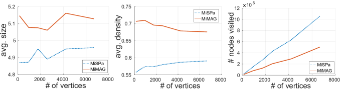
Figure 6. Size, Density, and number of visited nodes in the enumeration tree of MiSPa contrasted against MiMAG.

Given that MiSPa produces more patterns, it visits more nodes in the set enumeration tree (see right plot Fig. 6) but obtains fewer runtime. The underlying reason is that our used pruning techniques are more effective and efficient in sparse graphs. For example, some of the techniques discard unpromising nodes based on the graphs’ diameter (Pei et al., 2005); these principles are more expensive to compute in the dense complement graphs used in MiMAG and do not provide a significant pruning.

5.2. Evaluation on real-world datasets: Case Studies

Our next evaluation considers four real-world datasets. We provide case studies (Sec. 5.2) as well as overall statistics and performance results (Sec. 5.3).

Arxiv. The first real-world dataset considers a portion of the Arxiv database. Here, vertices of the graph are papers. For the first graph, two papers A and B are connected by an edge, if A cites or is being referenced by B. A second graph is constructed, considering the same papers, and computing the similarity of the abstracts. We used word2vec embeddings and cosine distance to measure similarity. Two papers are connected by an edge, if their similarity is larger than 0.98. In principle, papers with similar topics should be highly connected in the citation/reference graph.

So, our interest is to find similar papers without common cites, or cited papers in dissimilar topics. Overall, there are 6156 vertices and 20515 edges.

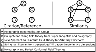
Figure 7. Papers with textual similarity and few citations/references.

Fig. 7 illustrates one contrasting pattern. Note five papers forming a 0.5-quasi-clique in the Similarity graph but with only few citations or references. Particularly, papers A, B, and D are highly related (forming a clique) to the Yang-Mill theory while the rest of them are partially similar and arise in the context of string theory. Despite the similarity, only papers A and B have a connection in the citation graph. The interestingness of the pattern is 3.

Friendship/Facebook. In the following experiment we have contrasted real-life friendship versus Facebook friendship among High School students, considering the data in (Mastrandrea et al., 2015). In this graph we have over 208 vertices and 1843 edges.

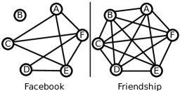
Figure 8. A CQC pattern w.r.t. friendship.

Fig. 8 exhibits a contrasting pattern where all six students have a real-life friendship, but they are very sparse in the Facebook graph. Interestingly, student B is not a Facebook friend of the other five students despite being a highly connected in the real-life graph. The interestingness of this pattern is 2.8.

DBLP. In our next case study, we have used a portion of the DBLP database. In this experiment, each author is a vertex of the KDD, ICDM, VLDB, ICML, WWW, and PAKDD venues, and there is an edge connecting two authors if they have co-authored at least two papers between the years 2000 and 2007. Likewise, a second graph is constructed considering co-authorship between 2008 and 2015. Intuitively, we aim at finding collaborations that start or end over time. This graph contains 5319 vertices and 7012 edges.

In Fig. 9 we can see an example of a collaboration that goes from sparse to highly dense. For example, Gupta and Gosh are no longer co-authors after 2007, in our co-authorship graph, and Gupta became connected with other Ghosh co-authors. By contrast, Ghosh remains collaborating with Dhillon and Deodhar. The interestingness of the pattern is 3.

Figure 9. A contrasting pattern in the co-authorship graphs.

	DBLP		Arxiv		Laws		Friendship
	MiSPa	MiMAG	MiSPa	MiMAG	MiSPa	MiMAG	MiSPa	MiMAG
runtime (min)	0.08	313.5	0.15	584.5	0.009	2.1	2.52	2.52
nodes visited $\times 10^{4}$	11.58	2.41	1.75	2.42	0.95	0.58	240.6	41.36
contrast: avg($I(O)$)	3.72	3.62	4.02	4.05	5.79	5.77	4.7	6.2
contrast: sum($I(O)$)	1255.7	698.6	1950	1200	81	75	539.7	254.4
density: avg($\gamma$)	0.57	0.74	1	1	0.78	0.85	0.86	0.88
size: avg(—O—)	5.32	5.38	4.04	4.04	5.12	6.84	5.55	7.22

Table 1. Performance on real data. MiSPa detects high contrast patterns with a significantly lower runtime.

Law data. Our last experiment comes from a collection of civil laws in Germany (the BGB). To construct this graph we have considered a law (i.e. a paragraph) as a vertex in the graph. In the first graph there is an edge connecting two laws, if one mentions (or is being mentioned by) the other. Then, we have extracted the top 21 keywords for each paragraph, and constructed a second graph by connecting two laws if they share at least 8 keywords. In principle, laws highly connected in the citation (reference) graph should also be textually related. Hence, the goal is to find dissimilar laws highly connected in the citation graph, and similar laws with fewer connections in the citation graph. Overall, the graph contains 2402 vertices and 3054 edges.

In Fig. 10 we illustrate one of these patterns. Notice that in terms of similarity the five laws form a 0.5-quasi-clique. This is expected since all these laws refer to the legal name of a child, so words like ’child’ or ’parent’ are very common.

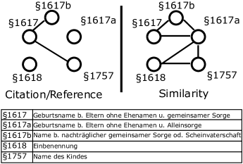
Figure 10. A collection of laws with few citations/references, but having high textual similarity.

Still, notice that $\S~{}1757$ and $\S~{}1617$ are textually dissimilar despite being connected in the Citation graph. This is because $\S~{}1757$ appears in the context of adoption while $\S~{}1617$ refers to the name of the child when one of the parents is not married to the biological parent of the child; i.e. the citation is expected. The interestingness of this pattern is 2.

5.3. Evaluation on real-world datasets: Overall performance

Running times and quality of the patterns. Table 1 summarizes the performance of our MiSPa algorithm and contrasts it against the complement graph approach with MiMAG as the quasi-clique detector.

Regarding runtime, our approach outperforms MiMAG (except in the small friendship graph). As discussed in Section 5.1, this result is related to the poor efficiency of MiMAG’s pruning techniques on dense (complement) graphs. Note that, with the exception of the Arxiv experiment, MiSPa visits more nodes in the enumeration tree which is expected since it considers more subtrees as potential CQC patterns and produces more of them.

Indeed, MiSPa generates often patterns with slightly higher interestingness and – despite its lower runtime – is able to find more interesting patterns, which is clearly illustrated in the sum of interestingness of all the patterns found, sum($I(O)$). In some cases (e.g. in the DBLP experiment) this amounts almost twice the number of patterns reported by MiMAG. In contrast to MiSPa, MiMAG is steered towards slightly more dense and large patterns since in almost all cases MiSPa reported patterns with less density and smaller.

5.4. Effectiveness of pruning

To test the effectiveness of our pruning and bounding techniques we have contrasted MiSPa with and without these techniques. In Fig. 11 we report the runtime and number of nodes visited in the set enumeration tree. Due to the exponential complexity of MiSPa without pruning strategies (see Sec. 4.3), we had to consider a smaller portion of the Arxiv, and the Facebook/Friendship datasets; the graphs have 4575 vertices/5837 edges, and 208 vertices/991 edges. To better illustrate the results we have plotted them using log scale.

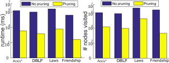
Figure 11. Runtime and number of visits to nodes in the enumeration tree of MiSPa with and without pruning techniques.

As shown in Fig. 11 (left) the runtime is dramatically affected without pruning. The Arxiv experiment took 443 times more time, the Conferences 676 times, the Law data experiment 420 times, and the Friendship experiment 1498 times. This can be explained by the number of visits made to the enumeration tree as shown in Fig. 11 (right). For example, without pruning, the Arxiv experiment did 74 times more visits and the Conferences experiment made 87 times more visits. Interestingly, the law data produces the highest number of visits and runtime despite being the second smallest in terms of number of edges and vertices (e.g. to find all contrasting patterns, it takes 2567 seconds without pruning techniques and only 6 seconds with pruning). These results show that the pruning techniques highly improve the performance of MiSPa.

Overall, as shown in these experiments, MiSPa successfully detects contrasting quasi-clique patterns in a variety of datasets. The various examples indicate the usefulness of our novel pattern model and the potential of MiSPa to efficiently find these patterns.

6. Conclusion

We proposed the new principle of contrasting quasi-clique patterns: subgraphs which are dense in one graph but sparse in another. Unlike existing works focusing on density only, our patterns highlight the difference/contrast between the subgraphs – thus, opening the door for a novel way of knowledge extraction. We introduced a model aiming to find a set of non-redundant, most interesting CQC patterns. Based on this model, we proposed an efficient A^∗-like algorithm using optimistic subtree estimates and pruning techniques. Using a variety of different real-world datasets we illustrated the efficiency of our method and how CQC patterns can be used to derive interesting insights from graphs.

While this paper introduced the first approach for finding CQC patterns, as future work we aim to derive even more scalable approaches, e.g., based on sampling, we plan to propose extensions to more complex multi-layer graphs, and to incorporate edge weights in the model.

References

- (1)
- Aggarwal and Wang (2010) C.C. Aggarwal and H. Wang. 2010. Managing and Mining Graph Data. Advances in Database Systems, Vol. 40. Springer, New York.
- Anchuri and Magdon-Ismail (2012) Pranay Anchuri and Malik Magdon-Ismail. 2012. Communities and balance in signed networks: A spectral approach. In ASONAM. 235–242.
- Boden et al. (2012) Brigitte Boden, Stephan Günnemann, Holger Hoffmann, and Thomas Seidl. 2012. Mining coherent subgraphs in multi-layer graphs with edge labels. In SIGKDD. 1258–1266.
- Cai et al. (2005) Deng Cai, Zheng Shao, Xiaofei He, Xifeng Yan, and Jiawei Han. 2005. Community Mining from Multi-relational Networks. In ECML PKDD. 445–452.
- Cerf et al. (2009a) Loïc Cerf, Jérémy Besson, Céline Robardet, and Jean-François Boulicaut. 2009a. Closed patterns meet n-ary relations. TKDD 3, 1 (2009).
- Cerf et al. (2009b) Loïc Cerf, Tran Bao Nhan Nguyen, and Jean-François Boulicaut. 2009b. Discovering Relevant Cross-Graph Cliques in Dynamic Networks. In ISMIS. 513–522.
- Esmailian and Jalili (2015) Pouya Esmailian and Mahdi Jalili. 2015. Community detection in signed networks: The role of negative ties in different scales. Scientific reports 5, 14339 (September 2015).
- Günnemann et al. (2010) Stephan Günnemann, Ines Färber, Brigitte Boden, and Thomas Seidl. 2010. Subspace Clustering Meets Dense Subgraph Mining: A Synthesis of Two Paradigms. In ICDM. 845–850.
- Jin and Wang (2011) Ning Jin and Wei Wang. 2011. LTS: Discriminative subgraph mining by learning from search history. In ICDE. 207–218.
- Kim and Lee (2015) Jungeun Kim and Jae-Gil Lee. 2015. Community Detection in Multi-Layer Graphs: A Survey. SIGMOD Rec. 44, 3 (December 2015), 37–48.
- Liu and Wong (2008) Guimei Liu and Limsoon Wong. 2008. Effective Pruning Techniques for Mining Quasi-Cliques. In ECML PKDD. 33–49.
- Mastrandrea et al. (2015) Rossana Mastrandrea, Julie Fournet, and Alain Barrat. 2015. Contact Patterns in a High School: A Comparison between Data Collected Using Wearable Sensors, Contact Diaries and Friendship Surveys. PLOS ONE 10, 9 (09 2015), 1–26.
- McAuley et al. (2015) Julian McAuley, Rahul Pandey, and Jure Leskovec. 2015. Inferring Networks of Substitutable and Complementary Products. In SIGKDD. 785–794.
- Moser et al. (2009) Flavia Moser, Recep Colak, Arash Rafiey, and Martin Ester. 2009. Mining Cohesive Patterns from Graphs with Feature Vectors. In SDM. 593–604.
- Müller et al. (2009) E. Müller, I. Assent, S. Günnemann, R. Krieger, and T. Seidl. 2009. Relevant subspace clustering: Mining the most interesting non-redundant concepts in high dimensional data. In ICDM. 377–386.
- Pei et al. (2005) J. Pei, D. Jiang, and A. Zhang. 2005. On mining cross-graph quasi-cliques. In SIGKDD. 228–238.
- Rymon (1992) Ron Rymon. 1992. Search through Systematic Set Enumeration. In KR. 539–550.
- Thoma et al. (2010) Marisa Thoma, Hong Cheng, Arthur Gretton, Jiawei Han, Hans-Peter Kriegel, Alex Smola, Le Song, Philip S Yu, Xifeng Yan, and Karsten M Borgwardt. 2010. Discriminative frequent subgraph mining with optimality guarantees. Statistical Analysis and Data Mining 3, 5 (2010), 302–318.
- Ting and Bailey (2006) Roger Ming Hieng Ting and James Bailey. 2006. Mining minimal contrast subgraph patterns. In SDM. 639–643.
- Uno (2010) Takeaki Uno. 2010. An Efficient Algorithm for Solving Pseudo Clique Enumeration Problem. Algorithmica 56, 1 (01 Jan 2010), 3–16.
- Wang et al. (2006) Jianyong Wang, Zhiping Zeng, and Lizhu Zhou. 2006. CLAN: An Algorithm for Mining Closed Cliques from Large Dense Graph Databases. In ICDE. 73–83.
- Zeng et al. (2006) Z. Zeng, J. Wang, L. Zhou, and G. Karypis. 2006. Coherent closed quasi-clique discovery from large dense graph databases. In SIGKDD. 797–802.