Spectral properties of MXB 1658–298 in the low/hard and high/soft state

Abstract

We report results from a broadband spectral analysis of the low mass X-ray binary MXB 1658–298 with the Swift/XRT and NuSTAR observations made during its 2015–2017 outburst. The source showed different spectral states and accretion rates during this outburst. The source was in low/hard state during 2015; and it was in high/soft state during the 2016 NuSTAR observations. This is the first time that a comparison of the soft and hard spectral states during an outburst is being reported in MXB 1658–298. Compared with the observation of 2015, the X-ray luminosity was about four times higher during 2016. The hard state spectrum can be well described with models consisting of a single-temperature blackbody component along with Comptonized disc emission, or three component model comprising of multi-colour disc, single-temperature blackbody and thermal Comptonization components. The soft state spectrum can be described with blackbody or disc blackbody and Comptonization component, where the neutron star surface (or boundary layer) is the dominant source for the Comptonization seed photons. We have also found a link between the spectral state of the source and the Fe K absorber. The absorption features due to highly ionized Fe were observed only in the soft state. This suggests a probable connection between accretion disc wind (or atmosphere) and spectral state (or accretion state) of MXB 1658–298.

1 Introduction

Low Mass X-ray Binaries (LMXBs) consist of a neutron star (NS) or a black hole (BH) with a low mass ($\lesssim 1M_{\sun}$) companion orbiting around it. The compact object accretes matter from its companion and the accretion rate is usually inferred from the position of the sources in their X-ray colour-colour diagrams (CDs) or hardness-intensity diagrams (HIDs) (Lewin & van der Klis, 2006). The low-luminosity sources trace out an atoll-like shape, with the different branches referred to as the banana branch (high inferred accretion rate) and the island state (low inferred accretion rate) (Hasinger & van der Klis, 1989). They have luminosity in the range of 0.001–0.5 $L_{Edd}$ (van der Klis, 2006).

The NS LMXBs display spectral states and hysteresis pattern similar to that observed in BH binaries, indicating similarity between these two kinds of sources (Muñoz-Darias et al., 2014). NS spectral emission is composed of three main components: disc blackbody from the accretion disc and Comptonization component due to Comptonization of soft X-rays in the corona as of the BH spectra (Done et al., 2007), with the addition of a blackbody component for emission from the NS surface or boundary layer (Lin et al., 2007, 2009; Armas Padilla et al., 2017). During the soft state, the emission is usually dominated by the thermal components, with characteristic temperatures of $kT\sim 0.5-2.0$ keV (Bloser et al., 2000a; Sakurai et al., 2012; Armas Padilla et al., 2017). The Comptonized component is weak with low temperature and large optical depth. In the hard state, the spectra are dominated by a hard Comptonized component with temperatures of a few tens of keV and low optical depths. The thermal components are observed at low temperatures ($kT<1$ keV) and with significantly lower luminosity (Raichur et al., 2011; Sakurai et al., 2012; Zhang et al., 2016; Armas Padilla et al., 2017).

Narrow absorption features from highly ionized Fe and other elements have been observed in large number of X-ray binaries. In particular, Fe xxv (He-like) or Fe xxvi (H-like) absorption lines near 6.6–7.0 keV have been reported from several NS LMXBs (e.g., Sidoli et al., 2001; Díaz Trigo et al., 2006; Hyodo et al., 2009; Ponti et al., 2014; Ponti et al., 2015; Raman et al., 2018) that are almost all viewed at fairly high inclination angles; most of them being dippers (Boirin et al., 2004, 2005; Díaz Trigo et al., 2006). This indicates that the highly ionized plasma probably originates in an accretion disc atmosphere or wind, which could be a common feature of accreting binaries but primarily detected in systems viewed close to edge-on (Díaz Trigo & Boirin, 2013, 2016).

MXB 1658–298 is a transient atoll NS LMXB system (Wijnands et al., 2002) which shows eclipses, dips and thermonuclear bursts in its X-ray lightcurves. It was discovered in 1976 with SAS-3 (Lewin et al., 1976). It has an orbital period of $\sim 7.1$ h and its eclipse lasts for $\sim 15$ min (Cominsky & Wood, 1984). This active phase lasted for about 2 years. The second outburst was observed in 1999–2001 (in ’t Zand et al., 1999b) during which coherent burst oscillations at frequency of $\sim 567$ Hz were reported (Wijnands et al., 2001). The 0.5–30 keV BeppoSAX spectrum obtained from observations made during this outburst, was modeled by a combination of a soft disc blackbody and a harder Comptonized component (Oosterbroek et al., 2001). The residuals to this fit suggested the presence of emission features due to Ne-K/Fe-L and Fe-K in the spectrum. The observations made with XMM-Newton revealed the presence of narrow resonant absorption features due to O viii, Ne x, Fe xxv and Fe xxvi, together with a broad Fe emission feature (Sidoli et al., 2001). The third outburst from the source was detected in the year 2015 (Negoro et al., 2015; Bahramian et al., 2015), which lasted for $\sim 1.5$ years (Parikh et al., 2017). The evolution of the orbital period over about 40 years of data indicates the presence of a circumbinary planet around this binary system (Jain et al., 2017).

In this work, we report results of spectral study of the persistent emission of MXB 1658–298 by using the Swift/XRT and NuSTAR observations made during 2015 and 2016. We also report the detection of state dependent absorption features due to highly ionized materials.

2 Observations and data reduction

The Nuclear Spectroscopic Telescope ARray (NuSTAR; Harrison et al., 2013) mission features two telescopes, focusing X-rays between 3 and 79 keV onto two identical focal planes (usually called focal plane modules A and B, or FPMA and FPMB). During its 2015–2017 outburst, MXB 1658–298 was observed twice with NuSTAR. The observation details are given in Table 1. We have used the most recent NuSTAR analysis software distributed with HEASOFT version 6.20 and the latest calibration files (version 20170120) for reduction and analysis of the NuSTAR data. The calibrated and screened event files have been generated by using the task nupipeline. A circular region of radius $100^{\prime\prime}$ centered at the source position was used to extract the source events. Background events were extracted from a circular region of same size away from the source. The task nuproduct was used to generate the lightcurves, spectra and response files. Using grppha, the spectra were grouped to give a minimum of 200 counts per bin. The FPMA/FPMB light curves were background-corrected and summed using lcmath. The persistent spectra were extracted by excluding the dips, eclipses and bursts.

Table 1: Log of X-ray observations.

Satellite	OBS Id	Start Time	Exposure∗	Mode
		(Date hh:mm:ss)	(ks)
NuSTAR	90101013002	2015-09-28 21:51:08	49.7	-
Swift/XRT	00081770001	2015-09-28 21:36:43	1.3	PC
NuSTAR	90201017002	2016-04-21 14:41:08	21.6	-
Swift/XRT	00081918001	2016-04-21 20:39:01	0.67	WT
∗Net exposure time of persistent emission.

MXB 1658–298 was also monitored by Neil Gehrels Swift Observatory (Gehrels et al., 2004) during its 2015–2017 outburst. For this work, we have focused only on those observations (listed in Table 1) which coincided with the NuSTAR observations. The Swift/X-ray telescope (XRT; Burrows et al., 2005) data were analysed using standard tools incorporated in HEASOFT version 6.20. The 2015 Swift/XRT observation was obtained in the PC mode wherein the effects of photon pile-up have been corrected. The 2016 observation was obtained in the WT mode and it was not affected by pile-up as the XRT count rate was $<100$ count/sec (Romano et al., 2006). We have used xselect to extract source events from a circular region of $70.8^{\prime\prime}$(=30 pixel) radius for WT mode; and annulus region of inner radius $10^{\prime\prime}$ and outer radius $100^{\prime\prime}$ for PC mode. Background events were obtained from the outer regions of the CCD. For the WT mode, we have extracted background from a region with same size of the source and for the PC mode, circular region of radius $150^{\prime\prime}$ was used. Exposure maps were used to create ancillary response files with xrtmkarf, to account for hot pixels and bad columns on the CCD. The latest response matrix file was sourced from the calibration data base (version 20160609). Spectra were grouped to contain a minimum of 20 counts per bin.

We have used XSPEC (Arnaud, 1996) version 12.9.1 for the spectral fitting. The persistent spectra extracted from Swift/XRT, NuSTAR-FPMA and NuSTAR-FPMB observations were fitted simultaneously. We have added a constant to account for cross-calibration of different instruments. The value of constant for NuSTAR-FPMA was fixed to 1 and set free for others. Due to the low energy spectral residuals in the WT mode, the WT mode data was fitted in the energy range 0.5–10 keV; and 0.3–10 keV energy range was used for PC mode data. The NuSTAR data in 3–70 keV and 3–35 keV energy range were used for spectral fitting for 2015 and 2016 observations, respectively. The photo-electric absorption cross section of Verner et al. (1996) and abundance of Wilms et al. (2000) have been used throughout. All the spectral uncertainties and the upper limits reported in this paper are at 90% confidence level. We have assumed the source distance to be equal to $10$ kpc (Muno et al., 2001; Sharma et al., 2018).

Figure 1: Background subtracted lightcurve of MXB 1658–298 extracted from 2015 (left) and 2016 (right) NuSTAR observations binned at 20 sec in energy band of 3–78 keV.

3 Lightcurve & Spectral States

Figure 1 shows the background subtracted FPMA+FPMB lightcurves of MXB 1658–298 binned at 20 sec in energy range of 3–78 keV extracted from NuSTAR observations of 2015 and 2016. During the 2015 observation, the background subtracted average count rate during the persistent phase was $\sim 6$ count/sec. One type-I thermonuclear X-ray burst was also observed where burst count rate reached $>500$ count/s (Sharma et al., 2018). During 2016, the background subtracted average persistent count rate increased to $\sim 40$ count/sec and the bursts observed were weaker and more frequent than 2015 observation.

The CD and HID for MXB 1658–298 are shown in Figure 2. They have been created after removing data during the bursts, dips and the eclipses. The soft colour corresponds to the ratio of count rate between 5–8 keV and 3–5 keV and the hard colour is the ratio between 12–30 keV and 8–12 keV. In Figure 2, the data points of 2015 and 2016 observations are denoted by black and red colours, respectively. In this figure, two branches are visible; the lower branch (red) can be identified with the banana branch and the upper (black) with the island state in CD (left panel of Figure 2). These different spectral branches depend on the accretion rates (Hasinger & van der Klis, 1989). Observation of 2015 shows low accretion state (island) and 2016 is showing high accretion state (banana), as shown in HID (right panel of Figure 2). For a quick comparison, the persistent spectrum for both observations is shown in Figure 3. It clearly shows that the spectrum of 2015 was low/hard and 2016 was high/soft.

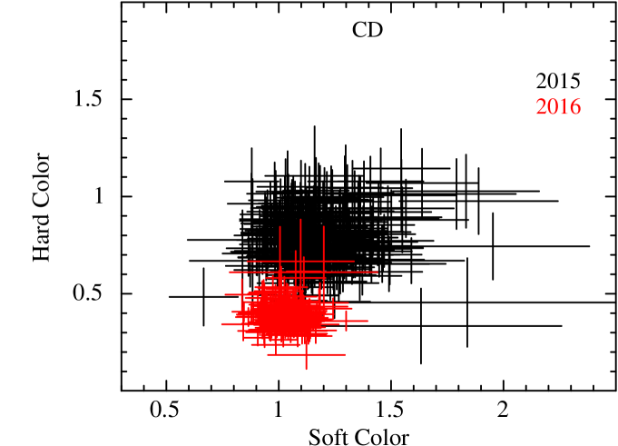
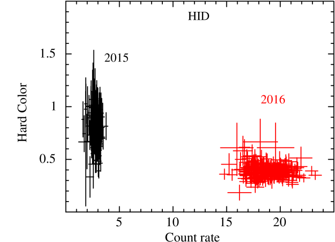
Figure 2: (left) Colour-colour diagram and (right) Hardness-intensity diagram of MXB 1658–298. The time resolution of the data is 200 sec and the count rate is in the energy range of 3–30 keV.

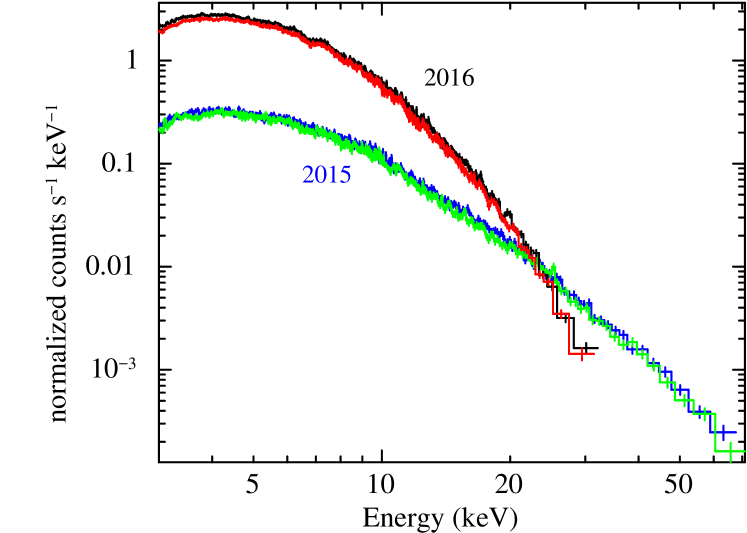
Figure 3: Persistent spectrum extracted from NuSTAR (FPMA & FPMB) observations of 2015 and 2016. The spectrum of 2015 was hard and had low flux emission while spectrum of 2016 was soft and had high flux emission. (The black and red colour represent the FPMA and FPMB data of 2016 observation, and blue and green represent FPMA and FPMB data of 2015 observation.)

4 Spectral Analysis and Results

Table 2: Spectral parameters of MXB 1658-298 obtained from the different best fit models in low/hard state.

Component	parameters	Model A1	Model A2	Model A3	Model A4
TBabs	$N_{H}(10^{22}~{}cm^{-2})$	$0.25\pm 0.07$	$<0.18$	$0.23^{+0.07}_{-0.06}$	$0.23^{+0.08}_{-0.06}$
diskbb	$kT_{disc}~{}(keV)$			$0.63^{+0.10}_{-0.08}$	$0.56^{+0.13}_{-0.12}$
	$Norm_{disc}$			$15.5^{+13.7}_{-7.4}$	$10^{+18}_{-6}$
bbodyrad	$kT_{BB}~{}(keV)$	$1.04\pm 0.04$	$1.04\pm 0.03$	$1.07^{+0.10}_{-0.08}$	$1.14^{+0.09}_{-0.08}$
	$Norm_{BB}$	$1.13\pm 0.17$	$1.13^{+0.17}_{-0.15}$	$1.46^{+0.58}_{-0.46}$	$0.80^{+0.27}_{-0.23}$
nthcomp	$\Gamma$	$1.74^{+0.01}_{-0.02}$		$1.71\pm 0.03$	$1.71\pm 0.03$
	$kT_{e}~{}(keV)$	$19.2^{+3.8}_{-2.3}$		$17.1^{+3.0}_{-2.0}$	$16.8^{+2.8}_{-1.9}$
	$kT_{seed}~{}(keV)$	$0.24~{}(<0.45)$		$=kT_{BB}$	$=kT_{disc}$
	input_type	1		0	1
	Norm ($\times 10^{-2}$)	$1.6^{+0.2}_{-0.3}$		$0.13\pm 0.13$	$1.05^{+0.22}_{-0.18}$
compTT	$kT_{e}~{}(keV)$		$14.8^{+1.6}_{-1.2}$
	$kT_{seed}~{}(keV)$		$0.28^{+0.05}_{-0.07}$
	$\tau$		$6.0\pm 0.4$
	Norm ($\times 10^{-3}$)		$2.1^{+0.5}_{-0.3}$
	${}^{a}frac_{disc}$	-	-	$0.20$	$0.08$
	${}^{a}frac_{BB}$	$0.05$	$0.06$	$0.08$	$0.06$
	${}^{a}frac_{comp}$	$0.95$	$0.94$	$0.72$	$0.86$
	†Flux${}_{0.5-10~{}keV}$	$1.15^{+0.05}_{-0.04}$	$1.06\pm 0.04$	$1.18\pm 0.01$	$1.18\pm 0.02$
	†Flux${}_{0.1-100~{}keV}$	$2.63^{+0.24}_{-0.08}$	$2.40^{+0.08}_{-0.07}$	$2.61\pm 0.05$	$2.61\pm 0.05$
	${}^{\dagger\dagger}L_{X}$	$3.15^{+0.29}_{-0.10}$	$2.87^{+0.09}_{-0.08}$	$3.12\pm 0.06$	$3.12\pm 0.06$
	$\chi^{2}/dof$	712.4/643	709/643	703.1/642	703.4/642
Model A1 : TBabs$\times$(bbodyrad+nthcomp[diskbb]);
Model A2 : TBabs$\times$(bbodyrad+compTT);
Model A3 : TBabs$\times$(diskbb+bbodyrad+nthcomp[BB]);
Model A4 : TBabs$\times$(diskbb+bbodyrad+nthcomp[diskbb]);
†Unabsorbed flux in units of $10^{-10}$ erg cm-2 s-1.
††Unabsorbed 0.1–100 keV X-ray Luminosity in units of $10^{36}$ erg s-1.
arepresents the component fraction.

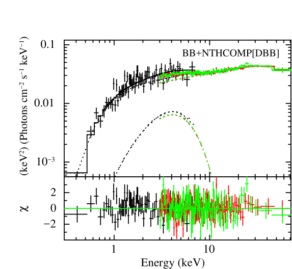
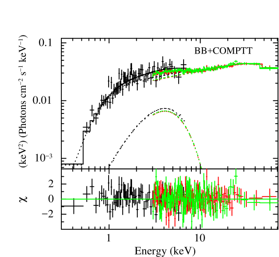
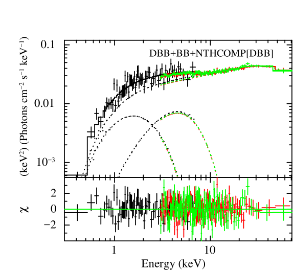
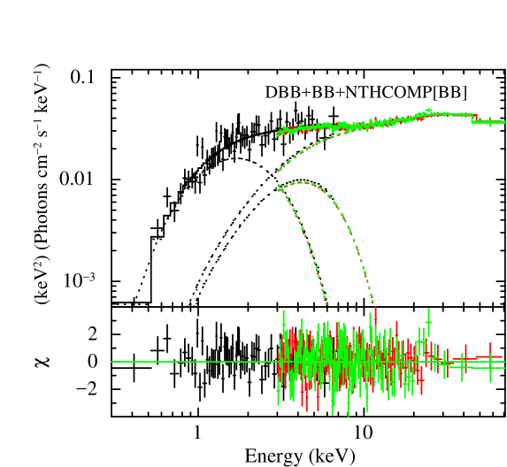
Figure 4: Spectrum of MXB 1658-298 extracted from 2015 observation (hard state) fitted with combinations of thermal and non-thermal components (model is mentioned on the top-right of each figure; DBB–diskbb, BB–bbodyrad). The NuSTAR data have been rebinned for representation purpose. The black points represent the Swift/XRT, red represent NuSTAR-FPMA and green represent NuSTAR-FPMB spectra.

The persistent emission spectra of MXB 1658–298 have been modeled with two component models (Oosterbroek et al., 2001; Sidoli et al., 2001; Díaz Trigo et al., 2006; Sharma et al., 2018). During the 1999–2001 outburst, MXB 1658–298’s broadband spectrum was studied with BeppoSAX and was modeled with combination of disc blackbody and Comptonization component (Oosterbroek et al., 2001). For the same outburst, the spectrum obtained from the observations made with XMM-Newton was modeled with combination of blackbody and cutoff power-law (Sidoli et al., 2001). In this work, we have modeled the persistent emission spectrum obtained from the observation of 2015 (low/hard) and 2016 (high/soft) with different combinations of continuum. This kind of comprehensive spectral analysis is being done for the first time in MXB 1658–298. We have tried single component models for the fitting the spectra of low/hard and high/soft states. But they do not provide statistically adequate fit in both the cases.

4.1 The Hard State Emission

We started with single-temperature blackbody (bbodyrad) plus exponential cutoff power-law (cutoffpl) to model the spectrum of 2015. TBabs has been used for modeling the interstellar absorption. The model TBabs $\times$ (bbodyrad+cutoffpl) did not give a good fit, $\chi^{2}=735$ for 644 degrees of freedom (dof).

Then, we replaced the cutoffpl component by the thermal Comptonization model nthcomp (Zdziarski et al., 1996; Życki et al., 1999). We have expressed the Comptonized model as nthcomp[BB] or nthcomp[diskbb], where [BB] means that seed photons are provided by blackbody and [diskbb] means that seed photons are provided by disc blackbody. A model comprising of the disc blackbody plus Comptonized blackbody gave unphysical value of inner disc radius and seed photon temperature ($kT_{seed}$). The Comptonized disc plus blackbody component (TBabs$\times$(bbodyrad+nthcomp[diskbb])) provided statistically good fit, $\chi^{2}/dof=712.4/643$ (model A1, see Table 2), where disc emission is completely Comptonized with $kT_{disc}=kT_{seed}=0.24(<0.45)$ keV. In model A1, nthcomp component specifies the Comptonization via coronal electron temperature $kT_{e}=19.2^{+3.8}_{-2.3}$ keV and the spectral slope $\Gamma=1.74^{+0.01}_{-0.02}$. Using the equation,

$$\centering\Gamma=-{1\over 2}+\sqrt{{9\over 4}+{1\over{kT_{e}\over m_{e}c^{2}}(1+{\tau\over 3})\tau}}\@add@centering$$

(see, Zdziarski et al., 1996) optical depth of Comptonizing corona estimated to $\tau\sim 4.1$. Following in ’t Zand et al. (1999a); Iaria et al. (2016), we have estimated the emission radius of seed photons (assuming a spherical emission) using

$$R_{0}=3\times 10^{4}D_{kpc}[f_{bol}/(1+y)]^{1/2}(kT_{seed})^{-2}~{}km,$$

where $D_{kpc}$ is the source distance in units of kpc, $f_{bol}$ is unabsorbed bolometric Comptonization flux and $y-$parameter is the Compton parameter defined as $y=4kT_{e}\tau^{2}/m_{e}c^{2}$ (relative energy gained by the photons in the inverse Compton scattering). Using best fit values, we obtained $y-$parameter $\sim 2.5$ and $R_{0}\sim 44(>12.5)$ km, where we used $f_{bol}$ to be 0.1–100 keV unabsorbed flux of Comptonized component ($=2.5\times 10^{-10}$ erg cm^-2 s^-1). The emission radius of seed photons is consistent with the seed photons being generated at the inner accretion disc. The $\sim 1$ keV blackbody with emission radius of $1.06\pm 0.08$ km suggests the emission from equatorial-belt like region of NS (Bloser et al., 2000a; Lin et al., 2007; Sakurai et al., 2012; Zhang et al., 2014).

We also examined the continuum with another thermal Comptonization model CompTT (Titarchuk, 1994) along with the same thermal components. CompTT model contains as free parameters; the temperature of the Comptonizing electron $kT_{e}$, the plasma optical depth $\tau$ and the input temperature of the soft photon (Wein) distribution $kT_{seed}$. A spherical geometry was assumed for the Comptonizing region (corona). The model TBabs $\times$ (bbodyrad + CompTT) provided us a marginally better fit, $\chi^{2}/dof=709/643$ (model A2, see Table 2).

We finally fit the spectrum with the three components model, composed by two thermal components (bbodyrad and diskbb) and Comptonization component, nthcomp[BB] (model A3) or nthcomp[diskbb] (model A4) (Lin et al., 2007; Armas Padilla et al., 2017). We obtained comparable chi-square values in the both cases. The best fit parameters obtained from the above described models are reported in Table 2. Figure 4 shows the best fit spectrum of MXB 1658–298 in the hard state from all the four best fit models explained above. We used the cflux convolution model in XSPEC to estimate the unabsorbed flux in the 0.5–10 keV and 0.1–100 keV energy range. The X-ray luminosities calculated from unabsorbed flux in the 0.1–100 keV energy range are reported in Table 2.

The inner disc radius $R_{in}$ can be estimated from diskbb normalization $Norm_{disc}$ using $R_{in}=\alpha\kappa^{2}(Norm_{disc}/cosi)^{1/2}D_{10kpc}$ km, where $D_{10kpc}$ is the distance to the source in units of 10 kpc and $i$ is the inclination angle of disc and $\alpha=0.41$ and $\kappa=1.7$ are correction factors (Kubota et al., 1998). The inner disc radius of $11^{+5}_{-3}$ and $9^{+8}_{-2}$ km is estimated for model A3 and A4, respectively assuming the inclination angle of $80^{\circ}$ (as source is eclipsing binary; Frank et al., 1987). The calculated inner disc radius is nearly the order of NS radius or close to NS. However, the value of the inner disc radius is uncertain, subjected to the uncertainty in the disc inclination angle $i$. The structure of Comptonized corona was same for both the cases and gave $y-$parameter$\sim 2.7$ and optical depth of $\sim 4.5$.

4.2 Soft State Emission

Table 3: Spectral parameters of MXB 1658-298 obtained from the different best fit models in high/soft state.

Component	parameters	Model B1	Model B2	Model B3
tbabs	$N_{H}(10^{22}~{}cm^{-2})$	$0.25\pm 0.05$	$<~{}0.05$	$0.26\pm 0.04$
edge	$E_{edge}~{}(keV)$	$7.72\pm 0.05$	$7.72\pm 0.05$	$7.73\pm 0.05$
	$\tau$	$0.162\pm 0.016$	$0.153^{+0.019}_{-0.014}$	$0.153^{+0.017}_{-0.018}$
edge	$E_{edge}~{}(keV)$	$9.07\pm 0.07$	$9.06\pm 0.07$	$9.06\pm 0.07$
	$\tau$	$0.129\pm 0.017$	$0.110^{+0.008}_{-0.017}$	$0.119^{+0.017}_{-0.016}$
gauss	$E_{line}~{}(keV)$	$6.77\pm 0.03$	$6.77\pm 0.03$	$6.77\pm 0.03$
	$width~{}(keV)$	$0.09^{+0.05}_{-0.09}$	$0.098^{+0.05}_{-0.08}$	$<0.13$
	Norm ($10^{-4}$)	$-2.98\pm 0.5$	$-3.1\pm 0.5$	$-2.87\pm 0.5$
	Eq. width (eV)	$-(52\pm 6)$	$-(54^{+8}_{-5})$	$-(50^{+18}_{-5})$
diskbb	$kT_{disc}~{}(keV)$			$0.94^{+0.11}_{-0.12}$
	Normdisc			$31^{+14}_{-9}$
bbodyrad	$kT_{BB}~{}(keV)$	$0.64\pm 0.04$	$0.54^{+0.02}_{-0.03}$
	NormBB	$55^{+21}_{-16}$	$247^{+53}_{-34}$
cutoffpl	$\Gamma$	$0.91\pm 0.08$
	$E_{c}~{}(keV)$	$5.3\pm 0.2$
	Norm	$0.11\pm 0.01$
nthcomp	$\Gamma$		$2.23^{+0.07}_{-0.06}$	$2.35\pm 0.16$
	$kT_{e}~{}(keV)$		$3.80^{+0.15}_{-0.12}$	$3.97^{+0.33}_{-0.25}$
	$kT_{seed}~{}(keV)$		$0.97^{+0.05}_{-0.09}$	$1.29^{+0.21}_{-0.24}$
	input_type		0	0
	Norm		$0.021^{+0.005}_{-0.004}$	$0.010^{+0.004}_{-0.003}$
	${}^{a}frac_{comp}$	$0.91$	$0.77$	$0.56$
	†Flux${}_{0.5-10~{}keV}$	$9.17\pm 0.22$	$8.33\pm 0.03$	$9.26\pm 0.04$
	†Flux${}_{0.1-100~{}keV}$	$11.7\pm 0.3$	$10.28\pm 0.04$	$11.71\pm 0.05$
	${}^{\dagger\dagger}L_{X}$	$13.99\pm 0.36$	$12.30\pm 0.05$	$14.01\pm 0.06$
	$\chi^{2}/dof$	857/840	846/839	861/839
Model B1 : TBabs$\times$edge$\times$edge$\times$(bbodyrad+cutoffpl+gaussian);
Model B2 : TBabs$\times$edge$\times$edge$\times$(bbodyrad+nthcomp[BB]+gaussian);
Model B3 : TBabs$\times$edge$\times$edge$\times$(diskbb+nthcomp[BB]+gaussian);
†Unabsorbed flux in units of $10^{-10}$ erg cm-2 s-1.
††Unabsorbed 0.1–100 keV X-ray luminosity in units of $10^{36}$ erg s-1.
arepresents the fraction of Comptonization/cutoffpl component.

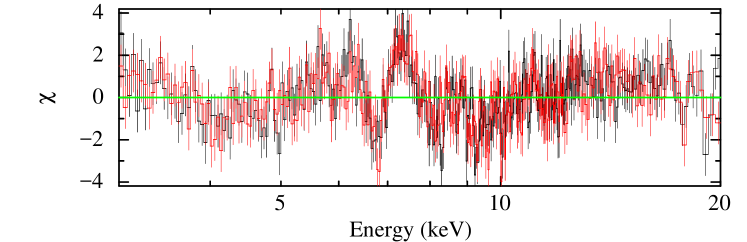
Figure 5: Residuals obtained after modeling persistent spectrum of 2016 observation with absorbed blackbody and cutoff power-law. For simplicity we have shown only NuSTAR data in 3–20 keV. These residuals indicate the absorption feature in 6–10 keV (absorption line and two absorption edges) mainly due to Fe K.

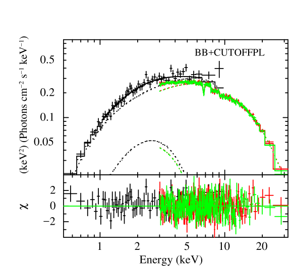
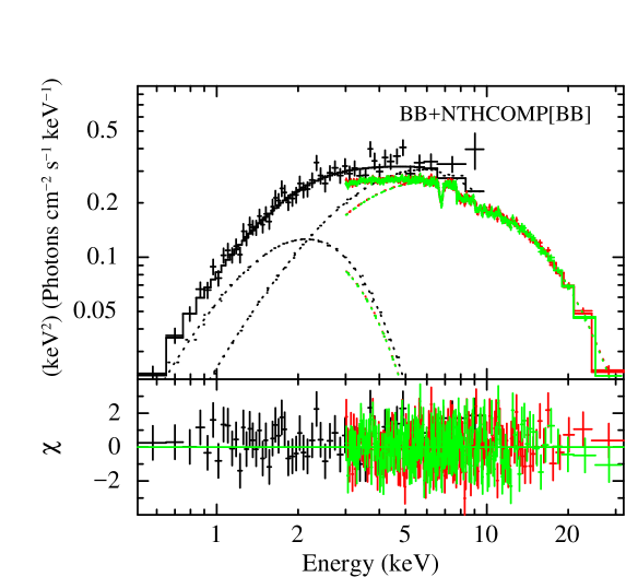
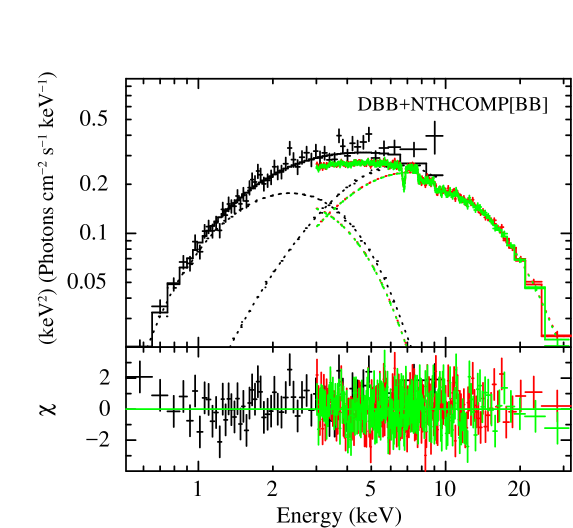
Figure 6: Spectrum of MXB 1658-298 extracted from 2016 observation (soft state) fitted with combinations of thermal and non-thermal components. The model is mentioned on the top-right of each figure. The colour scheme as described in Figure 4. The figures have been rebinned for representation purpose.

Table 4: Spectral parameters with single and double absorption detected in the high/soft state, where continuum used was TBabs$\times$(bbodyrad+nthcomp[BB]).

Component	Parameters	Single Absorption	Double Absorption
tbabs	$N_{H}(10^{22}~{}cm^{-2})$	$<0.05$	$<0.044$
edge 1	$E_{edge}~{}(keV)$	$7.72\pm 0.05$	$7.70\pm 0.05$
	$\tau$	$0.153^{+0.019}_{-0.014}$	$0.157^{+0.015}_{-0.014}$
edge 2	$E_{edge}~{}(keV)$	$9.06\pm 0.07$	$8.83^{f}$
	$\tau$	$0.110^{+0.008}_{-0.017}$	$0.057^{+0.025}_{-0.023}$
edge 3	$E_{edge}~{}(keV)$	-	$9.28^{f}$
	$\tau$	-	$0.062^{+0.024}_{-0.021}$
gauss 1	$E_{line}~{}(keV)$	$6.77\pm 0.03$	$6.70^{f}$
	$width~{}(keV)$	$0.098^{+0.05}_{-0.08}$	$0.05~{}(<0.13)$
	Norm ($10^{-4}$)	$-3.1\pm 0.5$	$-2.45^{+0.38}_{-0.59}$
	Eq. width (eV)	$-(54^{+8}_{-5})$	$-(43^{+8}_{-7})$
gauss 2	$E_{line}~{}(keV)$	-	$6.97^{f}$
	$width~{}(keV)$	-	$0.02~{}(<0.15)$
	Norm ($10^{-4}$)	-	$-0.93\pm 0.38$
	Eq. width (eV)	-	$-(18.6\pm 7.5)$
bbodyrad	$kT_{BB}~{}(keV)$	$0.54^{+0.02}_{-0.03}$	$0.55^{+0.02}_{-0.017}$
	NormBB	$247^{+53}_{-34}$	$244^{+45}_{-28}$
nthcomp	$\Gamma$	$2.23^{+0.07}_{-0.06}$	$2.23\pm 0.05$
	$kT_{e}~{}(keV)$	$3.80^{+0.15}_{-0.12}$	$3.80^{+0.12}_{-0.11}$
	$kT_{seed}~{}(keV)$	$0.97^{+0.05}_{-0.09}$	$0.99^{+0.10}_{-0.05}$
	input_type	0	0
	Norm	$0.021^{+0.005}_{-0.004}$	$0.020^{+0.003}_{-0.004}$
	$\chi^{2}/dof$	846/839	855/838
f Fixed.

During the observation of 2016, MXB 1658–298 was in the high/soft state and significantly detected above background upto 35 keV only. We have modeled the persistent spectra of 2016 observation with absorbed cutoff power-law with a thermal blackbody component, TBabs*(bbodyrad+cutoffpl). The fit obtained was unacceptable with $\chi^{2}/dof=1290/847$. This model described the 0.5–35 keV continuum well except between 6–10 keV. The structure of residuals showed the presence of an absorption line near 6.7 keV and two absorption edges at 7.7 keV and 9 keV (see, Figure 5). So we added a Gaussian absorption line model (gauss) and two absorption edge models (edge). This resulted in an acceptable fit with $\chi^{2}/dof=857/840$ (fit improvement by adding an edge at 9 keV: $-\Delta\chi^{2}=121$ for 2 additional parameters, another edge at 7.7 keV: $-\Delta\chi^{2}=143.7$ for 2 additional parameters and Gaussian absorption line at 6.7 keV: $-\Delta\chi^{2}=167.7$ for 3 additional parameters). The best fit parameters of this model (B1) are given in Table 3. With this model, the photon index obtained was hard ($\sim 0.91$). Similar hard photon index during soft state was found by Bloser et al. (2000a, b) with cutoff power-law model. If cutoffpl is replaced with powerlaw, the spectrum upto 10 keV will give photon index of $\sim 1.8$, consistent with the value measured in the soft state of NS LMXBs (Boirin et al., 2005; Díaz Trigo et al., 2006; Raman et al., 2018).

In the next approach, we replaced the cutoff power-law component with Comptonization component nthcomp. The model TBabs*(bbodyrad+nthcomp[BB or diskbb]) also showed the presence of same spectral feature of absorption in 6–10 keV. So, we added the same Gaussian absorption line and two absorption edge models. The model with nthcomp[diskbb] resulted in unphysical values of emission radius of disc photons $\sim 2-3$ km and $kT_{BB}<kT_{disc}$ (Lin et al., 2007). When input seed photon type changed to blackbody (nthcomp[BB]; model B2), an acceptable fit was obtained (Table 3).

We replaced the bbodyrad with diskbb in model B2. This gave a marginally poor fit but it describes the continuum well. This model (B3) represents the blackbody emission from NS surface/boundary layer with $kT_{BB}=1.29^{+0.21}_{-0.24}$ keV and emission radius of $R_{0}\sim 3-4$ km is completely Comptonized and emission from accretion disc with $kT_{disc}=0.94^{+0.11}_{-0.12}$ keV and inner disc radius of $R_{in}=15.8^{+3.7}_{-2.3}$ km is directly visible. We have also found that adding a third thermal component, diskbb in model B2 and bbodyrad in B3 did not improve the fit. So, the continuum during high/soft state can be described with combination of blackbody or disc blackbody and thermally Comptonization component where input seed photons are provided by blackbody (NS surface/boundary layer). Figure 6 shows the best fit spectrum of MXB 1658–298 in the soft state from above described best fit models B1, B2 and B3. The model TBabs $\times$ (bbodyrad+nthcomp[BB]) i.e., model B2 reproduce the data best as it improve the residuals in the soft band. The best fit parameters and the X-ray luminosities calculated from unabsorbed flux in the 0.1–100 keV energy range are reported in Table 3. The estimated X-ray luminosity during 2016 was a factor of $\sim 4$ higher than 2015.

Figure 7: Spectrum of MXB 1658–298 during high/soft state when modeled with double absorption. For representation purpose, figure has been rebinned and only NuSTAR data is shown.

4.2.1 Absorption features

The absorption line observed during soft state at $6.77\pm 0.03$ keV showed line width of $\sim 0.1$ keV and was broader than the results of the previous observations, when single absorption lines from Fe xxv and Fe xxvi were detected (Sidoli et al., 2001). This line can be due to blend of Fe xxv K$\alpha$ (6.70 keV) and Fe xxvi K$\alpha$ (6.97 keV) absorption lines. Accordingly, we applied two Gaussian absorption lines at 6.70 and 6.97 keV by freezing the line energy parameter instead of single Gaussian absorption line in the model B2. Both lines obtained were unresolved, we found the upper limits on the line widths of <0.12 keV and <0.14 keV for Fe xxv and Fe xxvi, respectively. The equivalent width (EW) of Fe xxv and xxvi K$\alpha$ lines obtained were $-42\pm 8$ eV and $-18\pm 7$ eV, respectively. The two absorption edges were observed at $7.72\pm 0.05$ keV and $9.06\pm 0.07$ keV with optical depth of $\sim 0.15$ and $0.11$, respectively. The absorption edge at 9 keV is due to highly ionized Fe xxv/xxvi K edge. Similar, absorption feature as observed in MXB 1658–298 were also observed in Galactic jet source GRO J1655–40 (Yamaoka et al., 2001). Since absorption line features of Fe K ions are detected, the accompanying absorption edge structures from the Fe ions in the same ionization states would also appear in the spectra. Hence following Yamaoka et al. (2001) and Sidoli et al. (2002), we applied two absorption edges fixed at 8.83 keV (Fe xxv) and 9.28 keV (Fe xxvi) instead of the single 9 keV edge detected above. The best-fit parameters for single and double absorptions are shown in Table 4. The obtained optical depth for 8.83 keV and 9.28 keV edges were nearly same $\sim 0.06$, shows both edges arises from nearly same region. Figure 7 shows the spectra with double absorption lines from Fe xxv and xxvi K$\alpha$ and their respective absorption edges.

The absorption lines due to Fe xxv K$\beta$ and Fe xxvi K$\beta$ at 7.88 keV and 8.26 keV, respectively had been observed in NS LMXB AX J1745.6–2901 (Hyodo et al., 2009; Ponti et al., 2015) and GX 13+1 (Sidoli et al., 2002). The observed absorption edge at 7.7 keV can be due to Fe xxv/xxvi K$\beta$ absorption lines with contribution from highly ionized Ni K$\alpha$ absorptions lines (Yamaoka et al., 2001) or(/and) Fe K emission as absorption edge can mimic the broad Fe K emission line (D’Aí et al., 2006; Egron et al., 2011; Mondal et al., 2016)

4.3 Photo-ionized Absorption Model

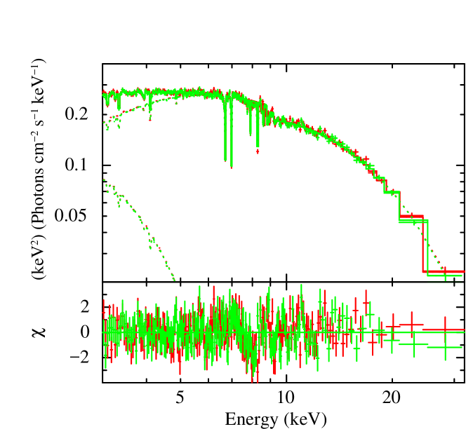
Figure 8: Spectrum when modeled with TBabs*zxipcf*(bbodyrad+nthcomp[BB]). For representation purpose, figure has been rebinned and only NuSTAR data is shown.

We have also modeled the observed absorption features in the soft state with a photo-ionized absorption component (zxipcf; Reeves et al., 2008) and assumed to be totally covering the X-ray source (covering fraction was fixed to 1). We modeled the broadband spectrum with model Tbabs*zxipcf*(bbodyrad+nthcomp[BB]). We note that zxipcf model was able to reproduce Fe K absorption lines between 6–7 keV and absorption edge at 9 keV (as shown in Figure 8). However residuals at 7–8 keV were still present. The fit showed positive residuals around 7 keV and negative residuals at 8 keV (see lower panel of Figure 8). The fit obtained was not good, $\chi^{2}/dof=927/844$. We first modeled these 7–8 keV features with an absorption edge. The fit improved to $\chi^{2}/dof=876.5/842$ with column density of $N_{H}\sim 10^{24}$ cm^-2 and ionization parameter of log$(\xi)\sim 4.2$ of ionized absorber. The absorption edge was observed at $7.53\pm 0.09$ keV with optical depth of $0.07\pm 0.01$. In the second approach, we modeled this feature with emission line using Gaussian model and fit improved to $\chi^{2}/dof=878/841$. The line energy observed was $6.78^{+0.06}_{-0.09}$ keV with line width of $0.38^{+0.11}_{-0.04}$ keV. The best fitting column density of ionized layer was $N_{H}=6.7^{+1.2}_{-2.4}\times 10^{23}$ cm^-2, having an ionization parameter log$(\xi)=4.06^{+0.09}_{-0.14}$. The EW of Fe K emission line obtained was $61^{+27}_{-20}$ eV. The edge at 7.5 keV can mimic the Fe K emission feature which was also found in 4U 1728–34 (D’Aí et al., 2006; Egron et al., 2011) and 4U 1820–30 (Mondal et al., 2016). Broad Fe K emission line was also observed during previous outburst with EW of $41^{+17}_{-9}$ eV in BeppoSAX spectra (Oosterbroek et al., 2001) and $160^{+60}_{-40}$ eV in XMM-Newton spectra (Sidoli et al., 2001).

4.3.1 Absorption in Hard State

Since no absorption feature were detected during persistent spectrum of 2015, therefore we added the Gaussian absorption line in model A1 to estimate upper limits. We found an absorption line at $6.63^{+0.13}_{-0.12}$ keV (line width fixed to 10 eV) with EW of $-15\pm 6$ eV with marginal fit improvement of $\Delta\chi^{2}=6$ for 2 additional parameters with F-test probability of 0.07. The addition of absorption line did not improve the fit significantly. So, this absorption feature is not much significant in this 2015 observation. We also estimated the upper limit on the EW of 6.4 keV Fe emission line of $16.5$ eV (line width fixed to 0.3 keV) and on 6.97 keV Fe xxvi absorption line of $-9$ eV (line width fixed to 10 eV). We have also modeled the persistent spectrum of 2015 with photo-ionization absorption model zxipcf. We used the resultant model Tbabs $\times$ zxipcf $\times$ (boodyrad + nthcomp[diskbb]). The covering fraction and redshift was fixed to 1 and zero, respectively. This improved the fit with $\Delta\chi^{2}=$4 for 2 additional parameters with F-test probability of 0.16, which is not significant. So during observation of 2015, no absorption features were detected significantly as observed in the observation of 2016.

5 Discussion and Conclusion

This work shows the comparison of the broadband spectrum of MXB 1658–298 in its soft and hard states. This kind of analysis has been done for the first time in this source. During its recent outburst, it was in low/hard state during the 2015 observation and in high/soft states during the 2016 observation. Many of the NS LMXBs have shown the transitions between the spectral states (Muñoz-Darias et al., 2014). Transient atoll source Aql X–1 has been observed in both hard and soft states during its 2007 outburst (Raichur et al., 2011; Sakurai et al., 2012). During the outburst of 2011, Aql X–1 is reported to show a spectral transition from hard to soft state (Ono et al., 2017). The transient LMXB AX J1745.6–2901 is also known to show both the spectral states during an outburst (Ponti et al., 2018).

During low/hard state, the combined broadband spectrum from NuSTAR and Swift/XRT observations can be well described with combination of thermal component (blackbody) and Comptonized disc component. However, combination of two thermal components (blackbody and disc blackbody) and Comptonized component can not be ruled out (see, Table 2). During 2016 observation when source was in high/soft state, its broadband spectrum can be described with combination of blackbody or disc blackbody and a Comptonization component (see, Table 3). In the soft state, our study supports the NS surface (or boundary layer) as the dominant source for the Comptonization seed photons yielding the observed weak hard emission, while in the hard state inner accretion disc is favoured but with three-component model solutions, either the disc or the NS surface/boundary layer are equally favoured. The spectral shape during both observations were different and were according to the spectral state of the source. The electron temperature of Comptonizing plasma decreased to $\sim 4$ keV in high/soft state from $\sim 19$ keV in low/hard state. During low/hard state, Comptonizing region had optical depth of $\sim 4.1$ and during high/soft state, plasma became optically thick with optical depth of $\sim$ 7. This type of variations in electron temperature and plasma optical depth have been observed during the hard and soft spectral state of several atoll LMXBs (e.g., Done et al., 2007; Raichur et al., 2011; Sakurai et al., 2012; Ono et al., 2017).

Like MXB 1658–298, the broadband spectrum of Aql X–1, a typical non-dipping LMXB and 4U 1915–05, a typical dipping LMXB were also modeled with diskbb+nthcomp[BB] model in the soft state (Sakurai et al., 2012; Zhang et al., 2014). They showed blackbody emission of $R_{BB}\sim 3-4$ km, which implies that the blackbody emission arises from an equatorial belt-like region on the NS surface. They also commonly indicate that the inner edge of the accretion disc is close to the NS surface ($R_{in}\sim 10-20$ km). The measured coronal temperature $kT_{e}$ of MXB 1658–298 $\sim 4$ keV, is somewhat higher than that of Aql X–1 ($2-3$ keV), but is significantly lower than 4U 1915–05 ($\sim 9$ keV) (Sakurai et al., 2012; Zhang et al., 2014). The dipping LMXBs in soft state (banana state) have systematically harder spectra than the normal LMXBs (Gladstone et al., 2007). The strength of Comptonization is normally evaluated by the $y-$parameter. Following Zhang et al. (2014), for LMXBs in the soft state, the difference between $kT_{e}$ and $kT_{seed}$ becomes small and they employed a new definition of the $y-$parameter as $4(\tau+\tau^{2}/3)(kT_{e}-kT_{seed})/m_{e}c^{2}$. The newly defined $y-$parameter of MXB 1658–298 is $\sim 0.5$ similar to 4U 1915–05 in the soft state (Zhang et al., 2014). This value appears at the upper limit of the recalculated $y-$parameters of normal LMXBs in the soft state by Zhang et al. (2014). Thus similar to 4U 1915–05, MXB 1658–298 is inferred to show stronger Comptonization effects than low and medium inclination LMXBs. We have obtained $y-$parameter $\sim 2.5$ in the hard state (as defined in section 4.1), a value higher than EXO 0748–676 ($y\sim 1.4$) and other low and medium inclined LMXBs ($y<1.4$; Zhang et al., 2016). The large difference in the value of $y-$parameter between MXB 1658–298 and EXO 0748–676 (both dipping LMXBs) can be due to the spectral modeling. EXO 0748–676 was modeled with diskbb+nthcomp[BB] (Zhang et al., 2016) while MXB 1658–298 was modeled with bbodyrad+nthcomp[diskbb]. Our model assume the the disc is fully covered by Comptonizing corona and the high value of $y-$parameter suggests that corona is flattened over the disc. So, our study suggests that the Comptonizing corona has an oblate shape and the seed photons have to pass through the corona with a longer path resulting in systematically stronger Comptonization (Zhang et al., 2014, 2016).

We have observed absorption lines due to highly ionized Fe K in MXB 1658–298 during high/soft state. The Fe xxv K$\alpha$ (6.70 keV) and Fe xxvi K$\alpha$ (6.97 keV) absorption lines were observed with EW of $-43^{+8}_{-7}$ eV and $-18.6\pm 7.5$ eV, respectively with their corresponding absorption edges with optical depth of $\sim 0.06$. For the first time absorption edges due to highly ionized Fe is observed in MXB 1658–298. The intense Fe K absorption features during soft states have been found in both NS and BH systems (e.g., Neilsen & Lee, 2009; Ponti et al., 2012, 2014, 2016; Ponti et al., 2018; Bozzo et al., 2016; Degenaar et al., 2014; Degenaar et al., 2016). The Fe K absorber is related to the presence of accretion disc absorber. In nearly 70% of the known NS LMXBs, absorbing material is known to be bound to the accretion disc atmosphere. There is no shift in their absorption line energies. The rest of systems show blueshift in their absorption line energies (Díaz Trigo & Boirin, 2013). For example, MXB 1658–298 (previous outburst), 4U 1323–62 and EXO 0748–676 did not show significant energy shifts, indicating that the absorption might occur in the disc atmosphere and does not necessarily require an outflow (Sidoli et al., 2001; Díaz Trigo et al., 2006; Boirin et al., 2005; Ponti et al., 2014). So, the observed absorption lines and edges in MXB 1658–298 are probably due to accretion disc atmosphere (or wind) as the source is viewed close to edge-on. Since, the observed K-absorption lines and K-absorption edges due to Fe ions were absent or not significantly detected during low/hard state. So, this suggests a connection between Fe K absorber and spectral state of the source. The connection between spectral state and presence of accretion disc wind or atmosphere have been found in both BH systems (Neilsen & Lee, 2009; Ponti et al., 2012) and high inclination NS LMXBs: EXO 0748–676 (Ponti et al., 2014) and AX J1745.6–2901 (Ponti et al., 2015, 2018). Our study presents an overall picture of high inclination LMXBs (BH and NS) and their spectral states/disc absorber connection.

References

- Armas Padilla et al. (2017) Armas Padilla M., Ueda Y., Hori T., Shidatsu M., Muñoz-Darias T., 2017, MNRAS, 467, 290
- Arnaud (1996) Arnaud K. A., 1996, in Jacoby G. H., Barnes J., eds, Astronomical Society of the Pacific Conference Series Vol. 101, Astronomical Data Analysis Software and Systems V. p. 17
- Bahramian et al. (2015) Bahramian A., Heinke C. O., Wijnands R., 2015, The Astronomer’s Telegram, 7957
- Bloser et al. (2000a) Bloser P. F., Grindlay J. E., Barret D., Boirin L., 2000a, ApJ, 542, 989
- Bloser et al. (2000b) Bloser P. F., Grindlay J. E., Kaaret P., Zhang W., Smale A. P., Barret D., 2000b, ApJ, 542, 1000
- Boirin et al. (2004) Boirin L., Parmar A. N., Barret D., Paltani S., 2004, Nuclear Physics B Proceedings Supplements, 132, 506
- Boirin et al. (2005) Boirin L., Méndez M., Díaz Trigo M., Parmar A. N., Kaastra J. S., 2005, A&A, 436, 195
- Bozzo et al. (2016) Bozzo E., et al., 2016, A&A, 589, A42
- Burrows et al. (2005) Burrows D. N., et al., 2005, Space Sci. Rev., 120, 165
- Cominsky & Wood (1984) Cominsky L. R., Wood K. S., 1984, ApJ, 283, 765
- D’Aí et al. (2006) D’Aí A., et al., 2006, A&A, 448, 817
- Degenaar et al. (2014) Degenaar N., Miller J. M., Harrison F. A., Kennea J. A., Kouveliotou C., Younes G., 2014, ApJ, 796, L9
- Degenaar et al. (2016) Degenaar N., et al., 2016, MNRAS, 461, 4049
- Díaz Trigo & Boirin (2013) Díaz Trigo M., Boirin L., 2013, Acta Polytechnica, 53, 659
- Díaz Trigo & Boirin (2016) Díaz Trigo M., Boirin L., 2016, Astronomische Nachrichten, 337, 368
- Díaz Trigo et al. (2006) Díaz Trigo M., Parmar A. N., Boirin L., Méndez M., Kaastra J. S., 2006, A&A, 445, 179
- Done et al. (2007) Done C., Gierliński M., Kubota A., 2007, A&ARv, 15, 1
- Egron et al. (2011) Egron E., et al., 2011, A&A, 530, A99
- Frank et al. (1987) Frank J., King A. R., Lasota J.-P., 1987, A&A, 178, 137
- Gehrels et al. (2004) Gehrels N., et al., 2004, ApJ, 611, 1005
- Gladstone et al. (2007) Gladstone J., Done C., Gierliński M., 2007, MNRAS, 378, 13
- Harrison et al. (2013) Harrison F. A., et al., 2013, ApJ, 770, 103
- Hasinger & van der Klis (1989) Hasinger G., van der Klis M., 1989, A&A, 225, 79
- Hyodo et al. (2009) Hyodo Y., Ueda Y., Yuasa T., Maeda Y., Makishima K., Koyama K., 2009, PASJ, 61, S99
- Iaria et al. (2016) Iaria R., et al., 2016, A&A, 596, A21
- Jain et al. (2017) Jain C., Paul B., Sharma R., Jaleel A., Dutta A., 2017, MNRAS, 468, L118
- Kubota et al. (1998) Kubota A., Tanaka Y., Makishima K., Ueda Y., Dotani T., Inoue H., Yamaoka K., 1998, PASJ, 50, 667
- Lewin & van der Klis (2006) Lewin W. H. G., van der Klis M., 2006, Compact Stellar X-ray Sources. Cambridge University Press
- Lewin et al. (1976) Lewin W. H. G., Hoffman J. A., Doty J., Liller W., 1976, IAU Circ., 2994
- Lin et al. (2007) Lin D., Remillard R. A., Homan J., 2007, ApJ, 667, 1073
- Lin et al. (2009) Lin D., Remillard R. A., Homan J., 2009, ApJ, 696, 1257
- Mondal et al. (2016) Mondal A. S., Dewangan G. C., Pahari M., Misra R., Kembhavi A. K., Raychaudhuri B., 2016, MNRAS, 461, 1917
- Muñoz-Darias et al. (2014) Muñoz-Darias T., Fender R. P., Motta S. E., Belloni T. M., 2014, MNRAS, 443, 3270
- Muno et al. (2001) Muno M. P., Chakrabarty D., Galloway D. K., Savov P., 2001, ApJ, 553, L157
- Negoro et al. (2015) Negoro H., et al., 2015, The Astronomer’s Telegram, 7943
- Neilsen & Lee (2009) Neilsen J., Lee J. C., 2009, Nature, 458, 481
- Ono et al. (2017) Ono K., Makishima K., Sakurai S., Zhang Z., Yamaoka K., Nakazawa K., 2017, PASJ, 69, 23
- Oosterbroek et al. (2001) Oosterbroek T., Parmar A. N., Sidoli L., in ’t Zand J. J. M., Heise J., 2001, A&A, 376, 532
- Parikh et al. (2017) Parikh A., Wijnands R., Bahramian A., Degenaar N., Heinke C., 2017, The Astronomer’s Telegram, 10169
- Ponti et al. (2012) Ponti G., Fender R. P., Begelman M. C., Dunn R. J. H., Neilsen J., Coriat M., 2012, MNRAS, 422, L11
- Ponti et al. (2014) Ponti G., Muñoz-Darias T., Fender R. P., 2014, MNRAS, 444, 1829
- Ponti et al. (2015) Ponti G., et al., 2015, MNRAS, 446, 1536
- Ponti et al. (2016) Ponti G., Bianchi S., Muñoz-Darias T., De K., Fender R., Merloni A., 2016, Astronomische Nachrichten, 337, 512
- Ponti et al. (2018) Ponti G., et al., 2018, MNRAS, 473, 2304
- Raichur et al. (2011) Raichur H., Misra R., Dewangan G., 2011, MNRAS, 416, 637
- Raman et al. (2018) Raman G., Maitra C., Paul B., 2018, MNRAS, 477, 5358
- Reeves et al. (2008) Reeves J., Done C., Pounds K., Terashima Y., Hayashida K., Anabuki N., Uchino M., Turner M., 2008, MNRAS, 385, L108
- Romano et al. (2006) Romano P., et al., 2006, A&A, 456, 917
- Sakurai et al. (2012) Sakurai S., Yamada S., Torii S., Noda H., Nakazawa K., Makishima K., Takahashi H., 2012, PASJ, 64, 72
- Sharma et al. (2018) Sharma R., Jaleel A., Jain C., Paul B., Dutta A., 2018, Journal of Astrophysics and Astronomy, 39, 16
- Sidoli et al. (2001) Sidoli L., Oosterbroek T., Parmar A. N., Lumb D., Erd C., 2001, A&A, 379, 540
- Sidoli et al. (2002) Sidoli L., Parmar A. N., Oosterbroek T., Lumb D., 2002, A&A, 385, 940
- Titarchuk (1994) Titarchuk L., 1994, ApJ, 434, 570
- Verner et al. (1996) Verner D. A., Ferland G. J., Korista K. T., Yakovlev D. G., 1996, ApJ, 465, 487
- Wijnands et al. (2001) Wijnands R., Strohmayer T., Franco L. M., 2001, ApJ, 549, L71
- Wijnands et al. (2002) Wijnands R., Muno M. P., Miller J. M., Franco L. M., Strohmayer T., Galloway D., Chakrabarty D., 2002, ApJ, 566, 1060
- Wilms et al. (2000) Wilms J., Allen A., McCray R., 2000, ApJ, 542, 914
- Yamaoka et al. (2001) Yamaoka K., Ueda Y., Inoue H., Nagase F., Ebisawa K., Kotani T., Tanaka Y., Zhang S. N., 2001, PASJ, 53, 179
- Zdziarski et al. (1996) Zdziarski A. A., Johnson W. N., Magdziarz P., 1996, MNRAS, 283, 193
- Zhang et al. (2014) Zhang Z., Makishima K., Sakurai S., Sasano M., Ono K., 2014, PASJ, 66, 120
- Zhang et al. (2016) Zhang Z., Sakurai S., Makishima K., Nakazawa K., Ono K., Yamada S., Xu H., 2016, ApJ, 823, 131
- Życki et al. (1999) Życki P. T., Done C., Smith D. A., 1999, MNRAS, 309, 561
- in ’t Zand et al. (1999a) in ’t Zand J. J. M., et al., 1999a, A&A, 345, 100
- in ’t Zand et al. (1999b) in ’t Zand J., Heise J., Smith M. J. S., Cocchi M., Natalucci L., Celidonio G., Augusteijn T., Freyhammer L., 1999b, IAU Circ., 7138
- van der Klis (2006) van der Klis M., 2006, in Lewin W., van der Klis M., eds, Compact Stellar X-ray Sources. Cambridge University Press. p. 39 (arXiv:astro-ph/0410551)