An alternative approach to the Finger of God in large scale structures

Abstract

It is generally accepted that linear theory of growth of structure under gravity produces a squashed structure in the two-point correlation function (2PCF) along the line of sight (LoS). On the other hand, the observed radial spread out structure known as Finger of God (FoG) is attributed to non-linear effects. In this paper we argue that the squashed structure associated with the redshift-space ($s-$) linear theory 2PCF is obtained only when this function is displayed in real-space ($r-$), or when the mapping from $r-$ to $s-$space is approximated. We find a way to solve for the mapping function $\bm{s}(\bm{r})$ that allows us to display the $s-$space 2PCF properly in a grid in $s-$space, by using plane of the sky projections of the $r-$ and $s-$ 2PCFs. We show that even in the simplest case of the linear Kaiser spectrum with a conservative power-law $r-$space 2PCF, a structure quite similar to the FoG is observed in the small scale region, while in the large scale the expected squashed structure is obtained. This structure depends on only three parameters.

Comúnmente se acepta que la teoría de colapso lineal gravitacional produce una estructura comprimida a lo largo de la visual en la función de correlación de dos puntos (2PCF). Por otro lado, la estructura conocida como Finger of God (FoG) se ha atribuido a efectos no-lineales. Aca argumentamos que la estructura asociada con el espacio de corrimiento al rojo ($s-$) de la 2PCF de la teoría lineal, sólo se obtiene cuando esta función es desplegada en el espacio-real ($r-$) ó cuando el mapeo de $r-$ al $s-$ se calcula mediante una aproximación. Encontramos una forma de resolver para la función de mapeo $\bm{s}(\bm{r})$ que nos permite visualizar correctamente la $s-$ 2PCF en una malla en $s-$, utilizando proyecciones en el plano del cielo para ambas 2PCFs, $r-$ y $s-$. Mostramos que aún en el caso mas simple, el de un espectro de Kaiser con ley de potencia para la 2PCF del $r-$, es posible apreciar a pequeña escala una estructura similar a FoG, mientras que a gran escala se obtiene la estructura comprimida esperada. Dicha estructura solo depende de tres parámetros.

galaxies: clusters: general galaxies: quasars: general cosmology: theory cosmology: large scale structure

0.1 Introduction

A spherical object observed at a distance in its longitudinal ($||$) and transversal ($\bot$) dimensions, should provide a test of different cosmological models, as first proposed by Alcock & Paczyński (1979). The Alcock-Paczyński parameter, hereafter $AP$, basically the ratio of $||$ to $\bot$ dimensions, takes a value of one at redshift zero, and increases with $z$ with a strong dependence on the value of the cosmological parameters that make up the Hubble function, introducing a cosmological distortion to the large scale structure observations. This apparently simple comparison is, however, greatly complicated by several factors. First, real-space measurements are not directly attainable and one has to rely on redshift-space. Then, if the proposed object consists of a cluster of quasars or galaxies, or a statistical ensemble of such, proper motions of its constituents, either derived from gravitational collapse or virialized conditions, distort redshift-space measurements causing a degeneracy problem (e.g., Hamilton, 1998). On cosmological scales, clusters of galaxies or quasars are among the most simple geometric structures that one may conceive. Even if single clusters may have non-spherical or filamentary structures, those should be randomly oriented. As we probe more distant clusters, observations become biased towards brighter and widely separated members, and the numbers become statistically insignificant. A superposition of many such clusters may reduce the problem while retaining spherical symmetry. The two-point correlation function (2PCF), and its Fourier transform, the power spectrum, have been fundamental tools in these studies for more than 40 years (e.g., Peebles, 1980).

Overdense clusters or associations separate from the Hubble flow due to their own gravity, which results in peculiar velocities of its members that distort redshift-space observations. When gravitational fields are small, velocities are well described by linear theory of gravitational collapse (Peebles, 1980). In the study of these clusters, the 2PCF was initially conceived as a single entity $\xi$ that could be evaluated in either real ($r-$) or redshift ($s-$) space (Peebles, 1980). Davis & Peebles (1983) even mentioned that when observing the local universe, if the peculiar velocities were small by comparison, $s-$space would directly reproduce $r-$space and one would have $\xi(\bm{r})=\xi(\bm{s})$. That should be the case for distant objects, although one should be careful not to mix up the notions of distant from each other and distant from the observer. In the case of the CfA Redshift Survey (e.g., Huchra et al., 1983), as described in Davis & Peebles (1983) peculiar velocities were significant, and the authors chose to go from real $\xi(r)$ to observable $\xi(s)$ by means of a convolution with a pair-wise velocity distribution, tailored to approach the Hubble flow at large distances, known as the streaming model. The convolution integral would at the same time convert $r-$space to $s-$space coordinates. However, the same function $\xi$ would be obtained as a result of the convolution of $\xi$ with a function of velocity, which constitutes an inconsistency. Later on, Kaiser (1987), hereafter K87, showed that gravitationally induced peculiar velocities by gravitational collapse of overdense structures in the linear regime, produces a power spectrum $P^{(s)}$ for $s-$space different from the one $P^{(r)}$ for $r-$space, that is two different functions for the power spectrum. Both are, however, functions of the $r-$space Fourier frequency $\bm{k}$. Then, while $P^{(r)}({\bm{k}})$ is a spherically symmetric function, $P^{(s)}({\bm{k}})$ shows an elongation along the line of sight (LoS) direction. Later on, Hamilton (1992) translated these results to configuration space obtaining the 2PCF in its two flavors: $\xi^{(r)}({\bm{r}})$ and $\xi^{(s)}({\bm{r}})$. Again $\xi^{(r)}({\bm{r}})$ is symmetric and the possibility of a power-law $r^{-\gamma}$ is considered, as had been historically accepted (e.g., Peebles, 1980, who favored $\gamma=1.8$ ). Also in perfect agreement with K87, $\xi^{(s)}({\bm{r}})$ shows a squashing along the LoS direction. Hamilton (1998) presents in great detail the assumptions that led to his results. He starts by defining selection functions $n^{(r)}(r)$ and $n^{(s)}(s)$ for $r-$space and $s-$space and by numerical conservation obtains a complicated high order expression (his eq. 4.28) for the density contrast $\delta^{(s)}$. From that one can obtain the 2PCF, but a series of approximations are needed (the linear case) first to reduce the right hand side of the equation and end up in his eq. 4.30 for $\delta^{(s)}({\bm{s}})$. Then, he performs one extra assumption, $\delta^{(s)}({\bm{r}})=\delta^{(s)}({\bm{s}})$, which is not justified by the linear approximation. This changes the left hand side of the equation directly to $\delta^{(s)}({\bm{r}})$. It may be argued that this approximation is valid in the distant case mentioned above. Consequently, one could easily write $\xi^{(s)}({\bm{s}})$ in place of $\xi^{(s)}({\bm{r}})$, shifting between one form and the other as needed. That is an imperative because observable 2PCF are inevitably obtained in $s-$space.

Since then many authors have tried the Kaiser linear approximation facing this dilemma and have performed similar approximations. In the description of 2PCF in redshift-space, due to the multipole expansion of the inverse Lagrangian operator derived from the corresponding power spectrum in Fourier space (Hamilton, 1992), there appears a dependence with $\mu$, the cosine of the angle between the ${\bm{r}}$ (real space) vector and the LoS: $\leavevmode\nobreak\ \mu{(\bm{r})}\,=\,r_{||}/|{\bm{r}}|$. However, it has been a common practice to approximate $\mu$ from redshift-space coordinates as either $\mu{(\bm{s})}=s_{||}/|{\bm{s}}|$ or $\mu{(\bm{cs})}=c_{||}s_{||}/\sqrt{c_{\bot}^{2}s_{\bot}^{2}+c_{||}^{2}s_{||}^{2}}$ (e.g., Matsubara & Suto, 1996; Nakamura et al., 1998; López-Corredoira, 2014). Yet in some other cases the approximation $r_{||}=s_{||}$ is specifically made (e.g.,, Tinker et al., 2006) calling it the “distant observer” approximation. But as mentioned above this is really meant to mean a wide separation approximation and does not apply in the small scale regime. Furthermore, the “distant observer” name is also used for the plane-parallel case (e.g., Percival & White, 2009), adding to confusion. In some other cases the substitution $r_{||}=s_{||}$ is just performed with no further comment (e.g., Hawkins et al., 2003). Another facet of the same problem has been to expand the redshift-space correlation function as a series of harmonics of that same $\mu{(\bm{s})}$, rather than the actual $\mu({\bm{r}})$ derived in linear theory (e.g., Guo et al., 2015; Chuang & Wang, 2012; Marulli et al., 2017). While this is certainly a valid approach, the conclusions of linear theory, like the existence of only monopole, quadrupole and hexadecapole terms in the Legendre polynomial expansion, are not really applicable to the $\mu{(\bm{s})}$ case. All these forms of the approximation are really one and the same, and to avoid further confusion (like the term “distant observer”) we decided to call it the $\mu(\bm{s})$ approximation.

When observational data is used to construct the 2PCF $\xi^{(s)}(\bm{s})$, it is generally true that simple linear theory predictions are not kept. On one hand, the predicted compression along the viewing direction is observed, but as one approaches the LoS axis the observed structure is mostly dominated by an elongated feature (e.g., Hamaus et al., 2015), usually called Finger of God (Huchra, 1988), hereafter FoG. Prominent examples of FoG were found in the Coma Cluster by de Lapparent et al. (1986) and in the Perseus cluster by Wegner et al. (1993). The FoG feature is also commonly observed in the 2PCF of statistical aggregates (e.g., Hawkins et al., 2003), making it a common feature in large scale structure.

Many studies have been conducted to explain this discrepancy. In general non-linear processes are invoked. Sometimes the non-linearities are assigned to virial relaxation in the inner regions of clusters, while others explore the non-linear terms in the approximation in the derivation of the K87 result. In these categories, we mention a small sample of representative literature. Kinematic relaxation, like the virialized motion of cluster members in the inner regions (Kaiser, 1987; Hamaus et al., 2015), are explored by introducing a distribution of pair-wise peculiar velocities for cluster components. There are at least two ways of doing so: First, the streaming model where a velocity distribution $f(V)$ is convolved with $\xi^{(r)}(\bm{r})$ to obtain $\xi^{(s)}(\bm{s})$, without using the K87 result, similar to Davis & Peebles (1983) but differentiating $\xi^{(s)}$ from $\xi^{(r)}$. More recent work on distribution functions take great care on this issue (Seljak & McDonald, 2011; Okumura et al., 2012a, b) by directly obtaining the power spectra in redshift-space as a function of the $s-$space wave-number. Unfortunately, the expression that results for the power spectra is rather complicated, even when it is conveniently expressed as a series in mass weighted velocity moments. However, it is possible to obtain FoG structures in $\xi^{(s)}(\bm{s})$ maps by the convolution with simple velocity distributions, at the same time that a mapping from $r-$ to $s-$space takes place (e.g., Scoccimarro, 2004). Paradoxically, it is not that easy to obtain the traditional peanut-shape structure that is generally recognized as the K87 limit in $\xi^{(s)}(\bm{s})$, unless the limit $s\sim r$ is once again invoked. Second, in the phenomenological dispersion model (c.f., Scoccimarro, 2004; Tinker et al., 2006) a linear K87 spectrum is multiplied in Fourier space by a velocity distribution. This can be seen as a convolution in configuration space, as in Hawkins et al. (2003), but the procedure has the disadvantage that it obtains the same function $\xi^{(s)}$ as the result of the convolution of $\xi^{(s)}$ and $f(V)$. It has to be noted, however, that very good fits to the observed data are obtained by this procedure. The same is true for the fits to numerical simulation results at mid spatial frequencies obtained by similar procedures in e.g., Marulli et al. (2017). In the streaming model, the velocity distribution function can also be obtained from the interaction of galaxies with dark mater halos (e.g., Tinker et al., 2006; Tinker, 2007), via the halo occupation distribution formalism.

Apart from kinematics, non-linear terms also arise in the expansion of the mass conservation or continuity equation in $r-$ and $s-$spaces to obtain the power spectrum or the 2PCF (e.g., Matsubara, 2008; Taruya et al., 2010; Zheng & Song, 2016). Preserving only first order terms yields the K87 result. However, a full treatment of all the terms is possible with the use of perturbative methods. There are diverse techniques: standard, Lagrangian, re-normalized, resumed Lagrangian (for a comparison see Percival & White, 2009; Reid & White, 2011). The latter authors however, conclude that the failure of these methods to fit the $l$=2 and 4 terms in the expansion $\xi^{(s)}_{l}(r)$ on quasi-linear scales of 30 to 80 $h^{-1}$ Mpc, must be due to inaccuracies in the mapping between $r$- and $s$-spaces. So, they favor again the streaming model. Clearly, there is still substantial debate on this subject.

In most of these works the necessity to translate their results to observable 2PCFs, $\xi^{(s)}(\bm{s})$, is not really addressed. Most authors prefer to display their results in Fourier space as $s$-space power spectrum $P^{(s)}(\bm{k}_{r})$ (e.g., Matsubara, 2008; Okumura et al., 2012a), but with $k_{r}$ in $r$-space; or display its moments $P^{(s)}_{l}(\bm{k}_{r})$ (e.g., Taruya et al., 2010; Zheng & Song, 2016); or power spectra with $k_{s}$ in $s-$space $P^{(s)}(\bm{k}_{s},\mu_{s})$ (e.g., Okumura et al., 2012b). Other authors display the correlation function in $r$-space, either as $\xi^{(r)}(\bm{r})$ (e.g., Matsubara, 2008) or $\xi^{(s)}(\bm{r})$ (e.g., Tinker, 2007; Reid & White, 2011; Okumura et al., 2012a), or its moments $\xi^{(s)}_{l}(s)$ (e.g., Taruya et al., 2010) for $l$=2. Few works try to display directly the 2PCFs $\xi^{(s)}(\bm{s})$ (e.g., Matsubara & Suto, 1996; Nakamura et al., 1998; Tinker et al., 2006; López-Corredoira, 2014), but as already mentioned above, usually perform the $\mu(\bm{s})$ approximation that amounts to really obtaining $\xi^{(s)}(\bm{r})$ instead.

To further complicate matters, redshift-space distortions are often treated separately from the cosmological distortions. Both are not easily discernible because both produce stretching or squashing in the LoS direction (Hamilton, 1998; Hamaus et al., 2015). This degeneracy could in principle be resolved because the cosmological and peculiar velocity signals evolve differently with redshift, but in practice the uncertain evolution of bias (the dimensionless growth rate for visible matter, see eq. 26) complicates the problem (Ballinger et al., 1996). Furthermore, Kaiser (1987) and Hamilton (1992, 1998) do not consider cosmological distortions in their analysis of peculiar motions. Since the earlier works, the inclusion of cosmological distortions has been attempted by several authors (e.g., Matsubara & Suto, 1996; Hamaus et al., 2015).

In this paper, we show that a structure quite similar to FoG can be obtained in $\xi^{(s)}(\bm{s})$ directly in the linear theory limit of K87. That is, without invoking virial relaxation or the streaming model, nor the non-linearities studied in perturbation theory, but just by avoiding the $\mu(\bm{s})$ approximation, in any of its forms ($\mu=s_{||}/|\bm{s}|$, “distant observer” or $r_{||}=s_{||}$ ), the FoG structure is recovered. This will be accomplished by solving for the function $\bm{r}(\bm{s})$ with the aid of the projected correlation function of both 2PCFs : $\xi^{(s)}(\bm{s})$ and $\xi^{(r)}(\bm{r})$. We will stay on the academic power-law approximation $\xi^{(r)}(\bm{r})\sim r^{-\gamma}$ in order to be able to show a closed form for the result, and to prove the main point of this paper, i.e. that the FoG feature is derived in the simplest case.

We start with a detailed definition of $r-$ and $s-$space, noting that frequently $s-$space is expressed in distance units as is $r-$space. But in doing so, one multiplies by a scale factor that invariably introduces a cosmological parameter in the definition; and as a result the named $s-$space is no longer purely observational. Later on the factor is solved by introducing a fiducial cosmology and solving for the real values. An example can be seen in the analysis made by Padmanabhan & White (2008) in Fourier space and Xu et al. (2013) in configuration space. The latter recognize the need of introducing a two-step transformation, one isotropic dilation and one warping transformation, to transform from real fiducial to real space. However, the real fiducial space is actually redshift-space, and this identification is missing in these works.

Therefore, we argue (c.f., Section 0.2) that it is convenient to define the observable-redshift-space ${\bm{\sigma}}$ (${\sigma}$-space) given by the simple redshift differences and subtended angles that are truly observable, and that do not depend on any choice of cosmological parameters. Multiplying by a units function (scale factor) produces the physical redshift-space ($s-$space): ${\bm{s}}=K({\bm{\Omega}},z)\leavevmode\nobreak\ {\bm{\sigma}}$, that is isomorphic to the observable ${\sigma}$-space, but has actual distance units that are dependent on a particular cosmological set of parameters Ω and the redshift $z$. The $K({\bm{\Omega}},z)$ function is chosen so that the physical redshift-space is related to real space ${\bm{r}}$ by a unitary Jacobian independent of redshift. So that no additional scaling is needed, and the only remaining difference will be precisely in shape. That is why ${\bm{\sigma}}$ and ${\bm{s}}$ are more alike, and thus can both be named redshift-space; ${\bm{\sigma}}$ is the observable redshift-space while ${\bm{s}}$ is the physical redshift-space. Then, the transformation to real-space necessarily goes through redshift distortions.

Furthermore, when we introduce peculiar non-relativistic velocities in this scheme, we will show that it is possible to keep the same relation between observable and physical redshift-spaces, ${\bm{s}}$ and ${\bm{\sigma}}$, and that the Kaiser (1987) effect is recovered independently of redshift (see Section 0.3). That is, now redshift-space will also show an additional gravitational distortion with respect to real-space.

To solve for the relation between real-space and redshift-space, we will rely on projected correlations. Projections of the 2PCF in the plane of the sky have been widely used to avoid the complications of dealing with unknown components in redshift-space (e.g., Davis & Peebles, 1983). This has the advantage that in the case of a symmetric 2PCF in real-space, the 3-D structure can be inferred from the projection. We will show in Section 0.4 that since the projections of the 2PCF in real-space and in redshift-space are bound to give the same profile, a relationship can be obtained for the real-space coordinate $r_{||}$ as a function of the corresponding one in redshift-space $s_{||}$. From this, we solve for $\mu{(\bm{r})}$ in real-space, and show that a different view of the redshift-space 2PCF emerges. The main result is that the redshift-space 2PCF presents a distortion in the LoS direction which looks similar to the ubiquitous FoG. This is due to a strong anisotropy that arises purely from linear theory and produces a change in scale as one moves into the on-axis LoS direction. As we move out of the LoS, a structure somewhat more squashed than the traditional result by the $\mu(\bm{s})$ approximation is obtained. As this effect has been missed before (to the best of our knowledge), we provide a detailed derivation in Sections 0.2 to 0.4, and show examples of the derived 2PCFs in redshift-space (Section 0.5). Finally, in Section 0.6 we summarize our main conclusions.

0.2 redshift-space

Consider the Friedmann-Lemaître-Robertson-Walker metric (e.g., Harrison, 1993) written in units of distance and time as follows:

$${ds}^{2}=c^{2}{dt}^{2}-dr^{2}=c^{2}{dt}^{2}-a(t)^{2}\left({d\chi}^{2}+S_{k}(\chi)^{2}({d\theta}^{2}+\sin^{2}(\theta){d\varphi}^{2})\right),$$ (1)

with   $S_{k}=(\leavevmode\nobreak\ sin\leavevmode\nobreak\ ,\leavevmode\nobreak\ {Identity}\leavevmode\nobreak\ ,\leavevmode\nobreak\ sinh\leavevmode\nobreak\ )$ for $k=(1,0,-1)$. Then the co-moving present-time length of an object $dr^{0}$ that is observed longitudinally is related to a variation in the observed redshift $dz$ by

$$dr_{||}^{0}=\frac{cdz}{H(z)},$$ (2)

where $H(z)$ is the Hubble function and the ⁰ superindex is used to define the present time $t_{0}$. Similarly, an object with a transversal co-moving dimension ${dr}_{\bot}^{0}$ subtends an angle $d\theta$ given by the angular co-moving distance (e.g., Hogg, 1999) as

$$\frac{{dr}_{\bot}^{0}}{{d\theta}}=a_{0}S_{k}\left(\frac{c}{a_{0}}\int_{0}^{z}\frac{{dz}^{\prime}}{H(z^{\prime})}\right),$$ (3)

where $a_{0}$ is the present day scaling parameter of the metric.

Observationally one measures redshift differences $dz$ and subtended angles $d\theta$. We then define the observable redshift-space adimensional quantities ($d\sigma_{||}\leavevmode\nobreak\ ,d\sigma_{\bot}$) as

$$d\sigma_{||}=dz$$ (4)

and

$$d\sigma_{\bot}=zd\theta.$$ (5)

The physical redshift-space sizes $ds_{||}$ and $ds_{\bot}$ can then be defined in terms of ${\bm{\sigma}}$ as

$$ds_{||}=K({\bm{\Omega}},z)d\sigma_{||}$$ (6)

and

$$ds_{\bot}=K({\bm{\Omega}},z)d\sigma_{\bot},$$ (7)

where $K({\bm{\Omega}},z)$ has distance units and depends on the cosmology, represented here symbolically by the ${\bm{\Omega}}$ terms. The relation between real-space and physical redshift-space is then obtained from eqs. (2) to (7), that is:

$$dr^{0}_{||}=c_{||}ds_{||}$$ (8)

and

$$dr^{0}_{\bot}=c_{\bot}ds_{\bot},$$ (9)

with

$$c_{||}=\frac{c}{K({\bm{\Omega}},z)\leavevmode\nobreak\ H(z)}$$ (10)

and

$$c_{\bot}=\frac{a_{0}}{z\leavevmode\nobreak\ K({\bm{\Omega}},z)}\leavevmode\nobreak\ S_{k}\left(\frac{c}{a_{0}}\int_{0}^{z}\frac{{dz}^{\prime}}{H(z^{\prime})}\right).$$ (11)

It is clear then that the Alcock & Paczyński (1979) function $AP(z)$, that tests redshift distortions of a particular cosmology, can be written as

$$AP(z)=\frac{c_{\bot}(z)}{c_{||}(z)}=\frac{a_{0}}{c}\leavevmode\nobreak\ \frac{H(z)}{z}\leavevmode\nobreak\ S_{k}\left(\frac{c}{a_{0}}\int_{0}^{z}\frac{{dz}^{\prime}}{H(z^{\prime})}\right).$$ (12)

Furthermore, from the transformation of physical redshift-space with coordinates $(ds_{\bot},ds_{\bot},ds_{||})$ into real-space $(dr_{\bot}^{0},dr_{\bot}^{0},dr_{||}^{0})$ we get a Jacobian

$$\left|{\frac{d^{3}\bm{s}}{d^{3}\bm{r}}}\right|=\frac{1}{c_{||}(z)}\leavevmode\nobreak\ \frac{1}{c_{\bot}^{2}(z)}.$$ (13)

In order for this transformation to preserve scale we need a unitary Jacobian. This condition can be achieved simply by the following condition:

$$K({\bm{\Omega}},z)=\frac{c}{H(z)}\leavevmode\nobreak\ AP(z)^{2/3},$$ (14)

as can be seen from eqs. (10) to (12). Here the dependence on the cosmology is made explicit through the Hubble function. Note that the resulting scale factor $K({\bm{\Omega}},z)$ approaches the Hubble radius $a_{H}=c/H_{0}$ as $z\rightarrow 0$ and decreases approximately as $1/(1+z)$ thereafter. Also note that for redshift $z>0$, the physical scale that transforms all dimensions of redshift-space, contracts isotropically. Also we remark that $c_{||}$ and $c_{\bot}$ are of order unity as $z\rightarrow 0$, and satisfy $c_{\bot}/c_{||}=AP(z)$ for all $z$. In fact we have (see also Xu et al., 2013):

$$c_{||}(z)=AP(z)^{-2/3},$$ (15)

and

$$c_{\bot}(z)=AP(z)^{1/3}.$$ (16)

Peculiar velocities modify the observed redshift, and therefore alter the relation between real-space and redshift-space giving rise to kinematic distortions. Suppose the near-end of an object is at rest at redshift $z$, while the far-end is moving with peculiar non-relativistic velocity $\vec{\rm v}$. Then it will appear Doppler shifted to an observer at rest at the far-end position, causing eq. (2) to get the form (see also Matsubara & Suto, 1996; Hamaus et al., 2015):

$$cdz=H(z)\leavevmode\nobreak\ dr_{||}^{0}+(1+z)\leavevmode\nobreak\ (\vec{\rm v}\cdot\hat{r}),$$ (17)

where $\hat{r}$ points in the direction of the far-end, at an angle $d\theta$ from the near-end. Since $\vec{\rm v}\cdot\hat{r}={\rm v}_{||}+{\rm v}_{\bot}\leavevmode\nobreak\ d\theta$, then for small angular separations ($d\theta<<1$) the perpendicular component of the peculiar velocity may be trivialized. Therefore eq. (8) gets modified to

$$dr_{||}^{0}=c_{||}\leavevmode\nobreak\ (ds_{||}-ds_{\rm v}).$$ (18)

where $ds_{\rm v}$ (in physical redshift-space) is given by

$$ds_{\rm v}=K({\bm{\Omega}},z)\leavevmode\nobreak\ d\sigma_{\rm v}$$ (19)

and $d\sigma_{v}$ (in observable redshift-space) is given by

$$d\sigma_{\rm v}=(1+z)\leavevmode\nobreak\ \frac{{\rm v}_{||}}{c}.$$ (20)

And through the similarity of eqs. (19) and (20) with eqs. (6) and (4), we note that the concepts of observable redshift-space and physical redshift-space can be extended to include peculiar motions as well.

0.3 Two point correlation function

Let ${\bm{r}}$ be real-space Euclidean co-moving coordinates in the close vicinity of a point at redshift $z$, what was defined as $dr$ in the previous section. Then for azimuthal symmetry around the line of sight (aligned to the third axis) we have ${\bm{r}}$ = $(dr_{\bot}^{0},dr_{\bot}^{0},dr_{||}^{0})$. Let ${\bm{s}}$ denote physical redshift-space coordinates around the same point (in the same tangent subspace), with the third axis along the line of sight. Then, from eqs. (9) and (18), the Jacobian is

$$\left|{\frac{d^{3}\bm{s}}{d^{3}\bm{r}}}\right|=\frac{1}{c_{||}(z)\leavevmode\nobreak\ c_{\bot}^{2}(z)}\leavevmode\nobreak\ \left(1+{\frac{(1+z)}{H(z)}}\leavevmode\nobreak\ \leavevmode\nobreak\ {\frac{\partial{\rm v}_{||}}{\partial r_{||}}}\right)=1+{\frac{(1+z)}{H(z)}}\leavevmode\nobreak\ \leavevmode\nobreak\ {\frac{\partial{\rm v}_{||}}{\partial r_{||}}},$$ (21)

where we have used the unitary condition on eq. (13) to eliminate the $c_{||}(z)\leavevmode\nobreak\ c_{\bot}^{2}(z)$ term. In going from ${\bm{r}}$ to ${\bm{s}}$ space, the density change can be related to the change in volume $V$, and the Jacobian by the equation

$$\left({\frac{d\rho}{\rho}}\right)_{\bm{s}-r}=-{\frac{dV}{V}}=1-\left|{\frac{d^{3}\bm{s}}{d^{3}\bm{r}}}\right|.$$ (22)

This can also be expressed in terms of the contrast density ratios in $\bm{s}$ and $\bm{r}$ spaces defined such that

$$\left({\frac{d\rho}{\rho}}\right)_{\bm{s}-r}=\delta^{(s)}-\delta^{(r)},$$ (23)

where $\delta^{(s)}$ and $\delta^{(r)}$ are two distinct scalar functions of position in either space. This particular definition of $\delta^{(s)}$ requires knowledge of the real-space selection function (Hamilton, 1998), which makes it rarely a first choice. However, the procedure given below allows us precisely to solve for the function ${\bm{r}}({\bm{s}})$.

In linear theory, Peebles (1980) shows in eqs. 14.2 and 14.8 that an overdensity of mass $\delta(\bm{r})$ creates a peculiar velocity field similar to the acceleration field produced by a mass distribution. As such, it can be derived from a potential function whose Laplacian is the overdensity itself (e.g., Thornton & Marion, 2004) times a constant which is time (or redshift) dependent. That is

$${\bf{\rm v}}({\bm{r}})=-{\frac{H(z)\leavevmode\nobreak\ f(z)}{(1+z)}}\leavevmode\nobreak\ {\bm{\nabla}}\nabla^{-2}\delta^{(r)}_{m}({\bm{r}}),$$ (24)

where $\nabla$ is the gradient and $\nabla^{-2}$ is inverse Laplacian, and

$$f(z)={\frac{a(z)}{D(z)}}{\frac{dD}{da}}.$$ (25)

Here $D(z)$ is the growth factor, the temporal component of density. Note that in Peebles (1980) coordinates are given in the expanding background model ${\bm{x}}$ which relate to present time real-space coordinates by ${\bm{r}}=a_{0}{\bm{x}}$; this brings about the $(1+z)$ factor to eq. (24). The $m$ subscript to $\delta$ emphasizes that all mass is responsible for the velocity field, while $\delta$ without the subscript refers to visible mass in the form of galaxies or quasars. To account for the difference, it is customary to introduce a bias factor $b(z)$ and define the dimensionless growth rate for visible matter

$$\beta(z)={\frac{f(z)}{b(z)}}.$$ (26)

Then from eqs. (21) to (24) we get:

$$\delta^{(s)}({\bm{r}})=\left(1+\beta(z)\leavevmode\nobreak\ \partial_{||}^{2}\leavevmode\nobreak\ \nabla^{-2}\right)\delta^{(r)}({\bm{r}}),$$ (27)

where $\partial_{||}$ denotes $\partial/\partial r_{||}$ in real space. Note that if we had not required a unity Jacobian (c.f., eq. 13), then eqs. (21) and (22) would not had canceled out the $1-c_{||}(z)^{-1}c_{\bot}(z)^{-2}$ term. We note that this term is not small when $K(\Omega,z)$ is a constant, and will vary by one order of magnitude as $z\rightarrow 1$, and up to three orders of magnitude as $z\rightarrow 10$. So the transformation between observable and physical redshift-spaces cannot be neglected (contrary to Matsubara & Suto, 1996, assumption).

The square modulus of the Fourier transform of eq. (27) gives an expression for the power spectrum, or the Fourier transform of the autocorrelation function (2PCF) $\xi$, which generalizes Kaiser (1987) results for any redshift $z$

$$\widetilde{\xi^{(s)}}({\bm{k}})=\left(1+\beta(z)\leavevmode\nobreak\ \mu_{k}^{2}\right)^{2}\widetilde{\xi^{(r)}}({\bm{k}}),$$ (28)

where $\mu_{k}=k_{r3}/|{\bm{k}_{r}}|$ is the cosine of the angle between the $k_{r3}$ component and the wave number vector ${\bm{k}_{r}}$ in real-space; and it arises by the Fourier transform property of changing differentials into products. Note that wave number vectors in real-space also differ from their counterparts in redshift-space by the unknown velocity field in eq. (17).

Fourier transforming back into coordinate space gives Hamilton (1992) result:

$$\xi^{(s)}({\bm{r}})=\left(1+\beta(z)\leavevmode\nobreak\ \partial_{||}^{2}\leavevmode\nobreak\ \nabla^{-2}\right)^{2}\xi^{(r)}({\bm{r}}).$$ (29)

Note that this equation is written in a way that all terms in the right hand side are real-space coordinates ${\bm{r}}$ dependent, as is the case for the derivatives and inverse Laplacian. Recalling that the solution of the Laplace equation in spherical coordinates consists of spherical harmonics in the angular coordinates and a power series in the radial part, one can write for the case of azimuthal symmetry

$$\xi^{(s)}({\bm{r}})=\sum_{l=0}\xi_{l}(r)\leavevmode\nobreak\ P_{l}(\mu{(\bm{r})})$$ (30)

where $P_{l}(\mu{(\bm{r})})$ are the Legendre polynomial,

$${\mu{(\bm{r})}}={\frac{r_{||}}{|{\bm{r}}|}},$$ (31)

explicitly defined for real-space coordinates, and the harmonics are given by the coefficients $\xi_{l}(r)$ that can be obtained from eq.(30) through orthogonality properties as

$$\xi_{l}(r)={\frac{(2l+1)}{2}}\int_{-1}^{1}P_{l}(\mu{(\bm{r})})\leavevmode\nobreak\ \xi^{(s)}({\bm{r}})\leavevmode\nobreak\ d\mu{(\bm{r})}.$$ (32)

Substituting eq. (29) in (32) for the case of spherical symmetry in real-space ($\xi^{(r)}({\bm{r}})=\xi^{(r)}(r)$), one gets by direct evaluation the classical result given by Hamilton (1992), see also Hawkins et al. (2003). That result consists of only three terms, monopole, quadrupole and hexadecapole ($l=0,2,4$), all the others evaluate to zero. It is important to note that this is not true when the expansion of eq. (30) has been done in $\mu{(\bm{s})}$ as is assumed by several authors (e.g., Guo et al., 2015; Chuang & Wang, 2012; Marulli et al., 2017).

When the 2PCF could be approximated by a power-law, $\xi^{(r)}(r)=(r/r_{0})^{-\gamma}$, the solution for eq. (29) can be written as

$$\xi^{(s)}({\bm{r}})=g(\gamma,\beta,\mu{(\bm{r})})\leavevmode\nobreak\ \xi^{(r)}(r).$$ (33)

where $g(\gamma,\beta,\mu{(\bm{r})})$ has been written in several equivalent forms (Hamilton, 1992; Matsubara & Suto, 1996; Hawkins et al., 2003). One of these is the following

$$g(\gamma,\beta,\mu{(\bm{r})})=1+2{\frac{1-\gamma\,\mu(\bm{r})^{2}}{3-\gamma}}\leavevmode\nobreak\ \beta(z)+{\frac{\gamma(\gamma+2)\,\mu(\bm{r})^{4}-6\gamma\,\mu(\bm{r})^{2}+3}{(3-\gamma)(5-\gamma)}}\leavevmode\nobreak\ \beta(z)^{2}.$$ (34)

This function takes values greater than 1 for the equatorial region ($\mu{(\bm{r})}\rightarrow 0$), and less than 1 for the polar axis ($\mu{(\bm{r})}\rightarrow 1$). Alternatively, it has been mentioned that the quadrupolar term in the multipole expansion dominates the hexadecapole. As a result of either argument the 2PCF $\xi^{(\bm{s})}(\bm{r})$ seems squashed with a peanut shape when displayed in $r$-space , in agreement with common knowledge.

However, we will show below that the stretching of redshift scale along the LoS will counteract this apparent squashing producing a structure similar to a FoG. In order to stay within the linear regime, we ensure not to reach the turnaround velocity by keeping $g(\gamma,\beta,\mu{(\bm{r})})$ positive in the polar region. In that case $\beta$ is limited from 0 to an upper limit which is a function of $\gamma$, and equals 2/3 when $\gamma=1.8$. The $\beta=0$ case gives the no gravity one in which $\xi^{(s)}({\bm{r}})=\xi^{(r)}({\bm{r}})$.

We now remark that $\mu{(\bm{r})}=r_{||}/|{\bm{r}}|$ (see eq. 31). But in some works (e.g., Matsubara & Suto, 1996; Tinker et al., 2006; López-Corredoira, 2014) it has been approximated as $\mu{(\bm{s})}=s_{||}/|{\bm{s}}|$ or as $\mu{(\bm{cs})}=c_{||}s_{||}/\sqrt{c_{\bot}^{2}s_{\bot}^{2}+c_{||}^{2}s_{||}^{2}},$ or even as $r_{||}=s_{||}$. We have referred to this as the $\mu{(\bm{s})}$ approximation. In principle, given that $\mu$ is a scalar function, either form should be acceptable as long as the ${\bm{s}}$ and ${\bm{r}}$ vectors refer to the same point. However, we remark that $r_{||}$ differs from $c_{||}s_{||}$ (see eq. 18), and that it is usually unknown, since in order to obtain it from $s_{||}$, the infall velocity field must be known. So these approximations should be carefully used.

The result in our eq. (33) has been derived for $r$-space, profiting on the difference between $r$- and $s$- spaces. Plotting this function directly in $r$-space as the independent variable, produces a squashed structure for $\xi^{(s)}(\bm{r})$. However, one wants to display the correlation function in $s$-space to compare with observations, not in $r$-space. In order to do so, some authors perform the $\mu(\bm{s})$ approximation while others may plainly substitute $s$ for $r$ all the way in eq. (33) and write $\xi^{(s)}(\bm{s})=g(\gamma,\beta,\mu(\bm{s}))\leavevmode\nobreak\ \xi^{(r)}(s)$ to be able to display $\xi^{(s)}$ in $s$-space. This is certainly wrong because $\bm{s}$ and $\bm{r}$ are not just independent names for position, and there exists a relation $\bm{s}(\bm{r})$ between them that is not linear. Specifically, the parallel component is $s_{||}\sim r_{||}+v_{||}$ (eq. 18), with $v_{||}$ also a (yet unknown) function of position $\bm{r}$. In the case of small disturbances we expect small velocities (below turnover) that result in a bi-univocal map $\bm{s}(\bm{r})$ and its inverse. So, if we want to display the resulting $\xi^{(s)}$ in $\bm{s}$ space, one must proceed first to evaluate $\bm{r}=\bm{r}(\bm{s})$ and then $\xi^{(s)}(\bm{r})$ via eq. (33), or in short $\xi^{(s)}(\bm{r}(\bm{s}))=g(\gamma,\beta,\mu(\bm{r}(\bm{s})))\leavevmode\nobreak\ \xi^{(r)}(r(\bm{s}))$. We can therefore informally define $\xi^{(s)}(\bm{s})\equiv\xi^{(s)}(\bm{r}(\bm{s}))$ and we claim that this is the correct way to evaluate the two-point correlation function on a grid in $s$-space.

On the other hand, if the $\mu{(\bm{s})}$ approximation is used one then obtains structures that are squashed in the LoS direction, and with a characteristic peanut-shaped geometry close to the polar axis (see for example Hawkins et al., 2003). One concludes that this geometry fails to reproduce the structure known as “Finger of God” (FoG). The consequence is that other processes are called upon to account for it, such as random motions arising in the virialized inner regions of clusters. We next show below that by avoiding this approximation, it allows us to obtain a geometrical structure quite similar to the FoG feature.

0.4 Projected correlation function

In order to avoid the complications that redshift-space distortions introduced in the correlation function, such as those produced by gravitationally induced motions or virialized conditions, the projected correlation function $w_{\bot}(r_{\bot})$ is frequently preferred in the analysis. This approach was first suggested in the analysis of CfA data by Davis & Peebles (1983), who mention that at small redshift separations, peculiar velocities may cause $\xi(s)$ to differ from $\xi(r)$. To avoid this effect, they integrate $\xi(r)$ along the redshift difference to obtain the projected function $w_{\bot}(r_{\bot})$ on the plane of the sky. Then, from it, they recuperate $\xi(r)$ inverting the problem by solving Abel’s integral equation (Binney & Tremaine, 1987) numerically. See also Pisani et al. (2014) for other possibilities. In the case where $\xi(r)$ is a power-law, $w_{\bot}(r_{\bot})$ will be one as well, and the relation between them is analytical (e.g., Krumpe et al., 2010).

We will show that the projected correlation function can be used to obtain the $r_{||}(s_{||})$ function that allows one to calculate $\mu{(\bm{r})}$. We start by noting that the projection on the plane of the sky may be performed either by using the $\xi^{(s)}$ function or its real space counterpart $\xi^{(r)}$. Then we define the projected correlation functions as

$$w^{(s)}_{\bot}(s_{\bot},s^{*}_{||})=\int_{0}^{s^{*}_{||}}{\xi^{(s)}({\bm{r}}(s_{\bot},s_{||}))\leavevmode\nobreak\ ds_{||}},$$ (35)

and

$$w^{(r)}_{\bot}(r_{\bot},r^{*}_{||})=\int_{0}^{r^{*}_{||}}{\xi^{(r)}(r_{\bot},r_{||})\leavevmode\nobreak\ dr_{||}},$$ (36)

where $\xi^{(s)}(\bm{r}(s_{\bot},s_{||})$, given by eq. (33), may be understood as $\xi^{(s)}(\bm{s})$ as mentioned above.

The integral limits should go to infinity to get the total projected functions. However, one can project the correlation function up to a particular real space distance $r^{*}_{||}$. Furthermore, if we assume that there exists a biunivocal function $s_{||}(r_{||})$, then we can find the corresponding $s^{*}_{||}=s_{||}(r^{*}_{||})$. Boundary conditions are thus well defined (e.g., Nock et al., 2010). On the one hand slices in r-space (eq. 36) do not depend on the observers perspective, while on the other (eq. 35) the limit of the integral (boundary condition) becomes a function that is precisely going to be evaluated. Carrying on, due to number conservation the projections in redshift- and real-space, multiplied by the corresponding area elements that complete the volume where the number of pairs are counted, must be equal. Which leads to

$$w^{(s)}_{\bot}(s_{\bot},s^{*}_{||})\leavevmode\nobreak\ ds_{\bot}^{2}=w^{(r)}_{\bot}(r_{\bot},r^{*}_{||})\leavevmode\nobreak\ dr_{\bot}^{2},$$ (37)

for all values of $r_{\bot}$ (or its corresponding $s_{\bot}$, see eq. 9). Inverting the $s_{||}(r_{||})$ map and using eqs. (35) to (37), together with (33) and (9) we obtain

$$\int_{0}^{s^{*}_{{||}}}{g(\gamma,\beta,\mu{(\bm{r})})\leavevmode\nobreak\ \xi^{(r)}(r_{\bot},r_{||})\leavevmode\nobreak\ ds_{||}}=c_{\bot}^{2}\leavevmode\nobreak\ \int_{0}^{r_{||}(s^{*}_{{||}})}{\xi^{(r)}(r_{\bot},r_{||})\leavevmode\nobreak\ dr_{||}}.$$ (38)

Then, changing variables to $r_{||}$ in the left ($ds_{||}={\frac{ds_{||}}{dr_{||}}}dr_{||}$), and noting that the equality holds for all values of $s^{*}_{{||}}$, the integral signs can be omitted. Furthermore, using eqs. (15) and (16) the equation simplifies to

$$c_{||}\leavevmode\nobreak\ ds_{||}={\frac{dr_{||}}{g(\gamma,\beta,\mu(\bm{r}(r_{\bot},r_{||})))}},$$ (39)

where the dependence $\mu(\bm{r}(r_{\bot},r_{||}))=r_{||}/\sqrt{r_{\bot}^{2}+r_{||}^{2}}$ has been emphasized for clarity. Equation (39) completes the metric transformation between redshift- and real-spaces. As a consistency test, we note that in the limit of no gravitational disturbance ($\beta=0$) we have $g(\gamma,\beta,\mu{(\bm{r})})=1$ and eq. (8) is recovered.

0.5 Resulting redshift-space and real-space relation

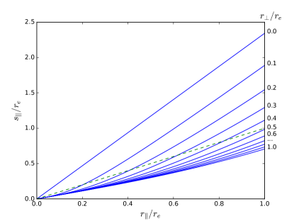
Figure 1: $s_{||}/r_{e}$ vs. $r_{||}/r_{e}$ for $r_{\bot}/r_{e}$ from 0 to 1 as indicated in the figure, for $\gamma=1.8$, $\beta=0.4$, and $c_{||}=1$. For any value of the scaling parameter $r_{e}$. The dashed line indicates the identity $s_{||}=r_{||}$ for reference.

We integrate eq. (39) numerically using eq. (34), to obtain the $s_{||}(r_{||})$ function shown in Figure 1, for different values of $r_{\bot}/r_{e}$ indicated for each curve in the figure, where $r_{e}$ is an arbitrary scaling parameter, $\gamma=1.8$, $\beta=0.4$, and $c_{||}=1$. Note that the relation is not linear. If we compare to the identity line ($s_{||}=r_{||}$) shown as a dashed line, we note that sometimes the curves of constant $r_{\bot}$ lie above or below the identity line, or even cross it.

So, it can be noted that for on-axis separations (where $r_{\bot}=0$), the spatial scale in redshift space is stretched, i.e. $s_{||}>r_{||}$, effectively opposing the squashing effect obtained by the rough $\mu{(\bm{s})}$ approximation. On the other hand, for $r_{\bot}\rightarrow 1$ a squashed structure is seen (even more so that the one obtained by the $\mu{(\bm{s})}$ approximation) that ultimately converges to the limit $s_{||}\rightarrow r_{||}$ as we approach the plane of the sky ($r_{||}=0$).

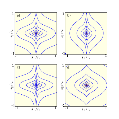
Figure 2: Redshift-space Two-Point-Correlation-Function (2PCF) $\xi^{(s)}(s_{\bot},s_{||})$ in logarithmically spaced contours at $e$ intervals for any value of the scaling parameter $r_{e}$. The parameter values are: a) $\gamma=1.8$, $\beta=0.4$ and $AP=1$; b) $\gamma=1.8$, $\beta=0.4$ and $AP=2$; c) $\gamma=1.8$, $\beta=0.5$ and $AP=1$; d) $\gamma=1.8$, $\beta=0.2$ and $AP=1$;

These geometrical distortions can be better appreciated by their effect on the 2PCF presented in Fig. 2. Here we start from a grid in $s-$space, and transform to r-space using the integral relation (eq. 39) for the parallel component and eq. (9) for the perpendicular one. From there, we calculate $\mu{(\bm{r})}$ (eq. 31), $g(\gamma,\beta,\mu{(\bm{r})})$ (eq. 34), assuming that $\xi^{(r)}({\bm{r}})=(r/r_{0})^{-\gamma}$; and finally, $\xi^{(s)}({\bm{s}})$ (i.e. $\xi^{(s)}(\bm{r}({\bm{s}}))$ ) from eq. (33). The cosmological distortion is governed by the $c_{||}$ and $c_{\bot}$ parameters that depend on the Alcock-Paczyński function $AP$ (see eq. 12). Its value depends on the cosmological parameters ${\bm{\Omega}}=(\Omega_{m},\Omega_{k},\Omega_{\Lambda})$ and increases with the redshift $z$ (see figure 1 in Alcock & Paczyński, 1979).

Figure 2(a) shows the case that corresponds to the parameters used for Figure 1: $\gamma=1.8$, $\beta=0.4$ and $AP=1$, where the geometrical distortions produced are evident, an elongation in the polar direction and a squashing in the equatorial direction. As can be noted the polar elongation resembles the structure known as FoG.

In the other three figures, 2(b), 2(c) and 2(d), we explore the effect of cosmological and gravitational alterations. Figure 2(b) shows that the effect of increasing $AP$ is a geometrical distortion that concentrates the structure towards the polar axis direction for $AP=2$ that corresponds to $\Lambda$CDM cosmology at $z=2.6$. In Figure 2(c) we explore the effect of changing the dimensionless growth-rate for visible mater $\beta$. This gravitational effect is to enhance the FoG structure as its value increases (recall that its limit value is 2/3). On the other hand, if $\beta$ decreases the structure becomes rounder and the FoG faints accordingly as is shown in Fig. 2(d). By comparing figures 2(b) and 2(c) relative to panel 2(a), we note that the same enhanced strength of the FoG feature is obtained in the small scale regions, but the large scale structure is quite different. This is because in the first case the distortion is cosmological while on the second it is gravitational.

Although it has not been the purpose of this paper, we may consider different values of the power-law index $\gamma$ and obtain figures similar to those shown in Fig. 2. In some cases they might even resemble some of the cases depicted here. It turns out that lower values may accommodate rounder 2PCFs at mid scales, while a steeper $\gamma$ may also concentrate the structure towards the LoS. Note however, that it is easy to discern those cases by a simple projection on the plane of the sky, as depicted through section 0.4. This is because that projection will erase redshift distortions, both gravitational ($\beta$) and cosmological ($AP$) while preserving the radial structure $\gamma$.

As we have indicated, a rounder 2PCF at mid spatial scales is favoured by some works that use the $\mu(s)$ approximation. As can be seen in Fig. 2(b), rounder figures can be obtained with lower values of $\beta$. We have estimated that a $\beta=0.25$ produces a 2PCF which is equally squashed to that obtained by the $\mu(s)$ approximation for the case $\beta=0.4$ for most points in the s-space plane, those with $s_{\bot}>s_{||}$. An increase in the $AP$ parameter may also contribute to alleviate the situation.

Another possibility, that was not intended to be covered here, is the case of a more realistic 2PCF $\xi^{(r)}({r})$ as the ones inferred from baryon acoustic oscillations (BAOs) (e.g. Slosar et al., 2013) or those obtained by the CAMB code (Seljak & Zaldarriaga, 1996). In order to apply the results of this paper to such cases, one could try breaking the inferred $\xi^{(r)}({r})$ profile in a series of power-laws and then apply eq. (39) to each section. If this is not possible, then we would have to give up eqs. (33) and (34) as a way of simplifying $\xi^{(s)}({\bm{r}})$. However, the projections in the plane of the sky, i.e. eqs. (35) and (36) are still valid, and instead of using eq. (33) to simplify, we would have to go back to the expansion of $\xi^{(s)}({\bm{r}})$ in multipoles eq. (30). In that case one would end up with the following equation:

$$c_{||}\leavevmode\nobreak\ ds_{||}={\frac{\xi^{(r)}(r)}{\sum_{l=0,2,4}\xi_{l}(r)\leavevmode\nobreak\ P_{l}(\mu{(\bf r)})}}dr_{||}$$ (40)

instead of eq. (39). And we would have to find a way to estimate the multipole moments $\xi_{l}(r)$. Another possibility is to leave $\xi^{(s)}(r)$ in the denominator. Considering these possibilities seems like an interesting task for future works, but it is beyond the scope of this paper.

We conclude that a whole range of possibilities in shape and strength of the FoG structure and the squashing of the equatorial zone can be obtained by tuning the parameters $\gamma$, $\beta$, and $AP$. This may provide a path towards solving the usual degeneracy problem between cosmological and gravitational distortions, that can still be seen at a level of 10% in 1$\sigma$ correlated variations in recent work (e.g. Satpathy et al., 2017).

0.6 Conclusions

We emphasize the importance of distinguishing three spaces in cluster and large scale structure studies: the observable redshift-space ${\bm{\sigma}}$, the physical redshift-space ${\bm{s}}$, and the real-space ${\bm{r}}$. The transformation between ${\bm{\sigma}}$ and ${\bm{s}}$ is isotropic dilation that introduces a scale factor dependent on the cosmology.

On the other hand, the transformation between ${\bm{s}}$ and ${\bm{r}}$ goes through a unitary Jacobian independent of redshift, and only distorts the space by factors related to the Alcock-Paczyński $AP$ function (c.f., eqs. 15 and 16).

Furthermore, when we introduce peculiar non-relativistic velocities in this scheme, we demonstrate that the same relation between observable and physical redshift-spaces ${\bm{s}}=K({\bm{\Omega}},z)\leavevmode\nobreak\ {\bm{\sigma}}$ is kept. In the analysis of the 2PCF in the physical redshift-space ${\bm{s}}$, we recover the Kaiser (1987) effect independent of redshift in Fourier space, and Hamilton (1992) results in configuration space.

We remark, that there appears a dependence with $\mu$ in real-space ($\mu{(\bm{r})}=r_{||}/|{\bm{r}}|$), and that it has been a common practice to approximate it from redshift-space coordinates as either $\mu{(\bm{s})}=s_{||}/|{\bm{s}}|$ or $\mu{(\bm{cs})}=c_{||}s_{||}/\sqrt{c_{\bot}^{2}s_{\bot}^{2}+c_{||}^{2}s_{||}^{2}}$ or $r_{||}=s_{||}$, sometimes called the“distant observer approximation”, or simply to substitute $\bm{s}$ for $\bm{r}$ in the equations. To avoid further confusion we have called this the $\mu{(\bm{s})}$ approximation in any of its forms. We argued that this wrong assumption produces either a squashed or a peanut-shaped geometry close to the LoS axis, for the 2PCF in redshift-space.

Since $r_{||}$ is usually unknown, we proposed a method to derive it from $s_{||}$ using number conservation in the projected correlation function in both real- and redshift-spaces. This led to a closed form eq. (39) for the case where the real 2PCF can be approximated by a power-law. From this, we solved for $\mu{(\bm{r})}$ in real-space, and showed that a different view of the redshift-space 2PCF emerges. The main result is that the redshift-space 2PCF presents a distortion in the LoS direction which looks quite similar to the ubiquitous FoG. This is due to a strong anisotropy that arises purely from linear theory and produces a stretching of the scale as one moves into the on-axis LoS direction. Moving away from the LoS the structures appear somewhat more squashed than those obtained by the $\mu(s)$ approximation for equivalent values of $\beta$. The implications of this remains an open question.

The development presented here produces structures that qualitatively reproduce the observed features of the 2PCF of galaxies and quasars large scale structure. A squashing distortion in the equatorial region is attributed to a mixture of cosmological and gravitational effects. And the FoG feature that is usually attributed to other causes, is instead ascribed to the same gravitational effects derived from linear theory.

We conclude that a whole range of possibilities in shape and strength of the FoG structure, and the squashing of the equatorial zone, can be obtained by tuning the parameters $\gamma$, $\beta$, and $AP$. This provides a path towards solving the usual degeneracy problem between cosmological and gravitational distortions. In a future paper (Salas & Cruz-González in preparation) we apply these results to the galaxies and quasar data obtained by current large scale surveys.

Acknowledgements. I.C.G. acknowledges support from DGAPA-UNAM (Mexico) grant IN113417.

References

- Alcock & Paczyński (1979) Alcock, C. & Paczyński, B. 1979, Nature, 281, 358
- Ballinger et al. (1996) Ballinger, W. E., Peacock, J. A., & Heavens, A. F. 1996, MNRAS, 282, 877
- Binney & Tremaine (1987) Binney, J. & Tremaine, S. 1987, Galactic Dynamics (Princeton University Press)
- Chuang & Wang (2012) Chuang, C.-H. & Wang, Y. 2012, MNRAS, 426, 226
- Davis & Peebles (1983) Davis, M. & Peebles, P. J. E. 1983, ApJ, 267, 465
- de Lapparent et al. (1986) de Lapparent, V., Geller, M. J., & Huchra, J. P. 1986, ApJ Letters, 302, L1
- Guo et al. (2015) Guo, H., Zheng, Z., Zehavi, I., Dawson, K., Skibba, R. A., Tinker, J. L., Weinberg, D. H., White, M., & Schneider, D. P. 2015, MNRAS, 446, 578
- Hamaus et al. (2015) Hamaus, N., Sutter, P. M., Lavaux, G., & Wandelt, B. D. 2015, J. Cosmology Astropart. Phys., 11, 036
- Hamilton (1992) Hamilton, A. J. S. 1992, ApJ Letters, 385, L5
- Hamilton (1998) Hamilton, D., ed. 1998, Astrophysics and Space Science Library, Vol. 231, Linear Redshift Distortions: a Review, ed. D. Hamilton, 185
- Harrison (1993) Harrison, E. 1993, ApJ, 403, 28
- Hawkins et al. (2003) Hawkins, E., Maddox, S., Cole, S., Lahav, O., Madgwick, D. S., Norberg, P., Peacock, J. A., Baldry, I. K., Baugh, C. M., Bland-Hawthorn, J., Bridges, T., Cannon, R., Colless, M., Collins, C., Couch, W., Dalton, G., De Propris, R., Driver, S. P., Efstathiou, G., Ellis, R. S., Frenk, C. S., Glazebrook, K., Jackson, C., Jones, B., Lewis, I., Lumsden, S., Percival, W., Peterson, B. A., Sutherland, W., & Taylor, K. 2003, MNRAS, 346, 78
- Hogg (1999) Hogg, D. W. 1999, ArXiv Astrophysics e-prints /9905116
- Huchra et al. (1983) Huchra, J., Davis, M., Latham, D., & Tonry, J. 1983, ApJS, 52, 89
- Huchra (1988) Huchra, J. P. 1988, in Astronomical Society of the Pacific Conference Series, Vol. 5, The Minnesota lectures on Clusters of Galaxies and Large-Scale Structure, ed. J. M. Dickey, 41–70
- Kaiser (1987) Kaiser, N. 1987, MNRAS, 227, 1
- Krumpe et al. (2010) Krumpe, M., Miyaji, T., & Coil, A. L. 2010, ApJ, 713, 558
- López-Corredoira (2014) López-Corredoira, M. 2014, ApJ, 781, 96
- Marulli et al. (2017) Marulli, F., Veropalumbo, A., Moscardini, L., Cimatti, A., & Dolag, K. 2017, A&A, 599, A106
- Matsubara (2008) Matsubara, T. 2008, Physical Review D, 77, 063530
- Matsubara & Suto (1996) Matsubara, T. & Suto, Y. 1996, ApJ Letters, 470, L1
- Nakamura et al. (1998) Nakamura, T. T., Matsubara, T., & Suto, Y. 1998, ApJ, 494, 13
- Nock et al. (2010) Nock, K., Percival, W. J., & Ross, A. J. 2010, MNRAS, 407, 520
- Okumura et al. (2012a) Okumura, T., Seljak, U., & Desjacques, V. 2012a, J. Cosmology Astropart. Phys., 11, 014
- Okumura et al. (2012b) Okumura, T., Seljak, U., McDonald, P., & Desjacques, V. 2012b, J. Cosmology Astropart. Phys., 2, 010
- Padmanabhan & White (2008) Padmanabhan, N. & White, M. 2008, Physical Review D, 77, 123540
- Peebles (1980) Peebles, P. J. E. 1980, The large-scale structure of the universe (Princeton University Press)
- Percival & White (2009) Percival, W. J. & White, M. 2009, MNRAS, 393, 297
- Pisani et al. (2014) Pisani, A., Lavaux, G., Sutter, P. M., & Wandelt, B. D. 2014, MNRAS, 443, 3238
- Reid & White (2011) Reid, B. A. & White, M. 2011, MNRAS, 417, 1913
- Satpathy et al. (2017) Satpathy, S., Alam, S., Ho, S., White, M., Bahcall, N. A., Beutler, F., Brownstein, J. R., Chuang, C.-H., Eisenstein, D. J., Grieb, J. N., Kitaura, F., Olmstead, M. D., Percival, W. J., Salazar-Albornoz, S., Sánchez, A. G., Seo, H.-J., Thomas, D., Tinker, J. L., & Tojeiro, R. 2017, MNRAS, 469, 1369
- Scoccimarro (2004) Scoccimarro, R. 2004, Physical Review D, 70, 083007
- Seljak & McDonald (2011) Seljak, U. & McDonald, P. 2011, J. Cosmology Astropart. Phys., 11, 039
- Seljak & Zaldarriaga (1996) Seljak, U. & Zaldarriaga, M. 1996, ApJ, 469, 437
- Slosar et al. (2013) Slosar, A., Iršič, V., Kirkby, D., Bailey, S., Busca, N. G., Delubac, T., Rich, J., Aubourg, É., Bautista, J. E., Bhardwaj, V., Blomqvist, M., Bolton, A. S., Bovy, J., Brownstein, J., Carithers, B., Croft, R. A. C., Dawson, K. S., Font-Ribera, A., Le Goff, J.-M., Ho, S., Honscheid, K., Lee, K.-G., Margala, D., McDonald, P., Medolin, B., Miralda-Escudé, J., Myers, A. D., Nichol, R. C., Noterdaeme, P., Palanque-Delabrouille, N., Pâris, I., Petitjean, P., Pieri, M. M., Piškur, Y., Roe, N. A., Ross, N. P., Rossi, G., Schlegel, D. J., Schneider, D. P., Suzuki, N., Sheldon, E. S., Seljak, U., Viel, M., Weinberg, D. H., & Yèche, C. 2013, J. Cosmology Astropart. Phys., 4, 026
- Taruya et al. (2010) Taruya, A., Nishimichi, T., & Saito, S. 2010, Physical Review D, 82, 063522
- Thornton & Marion (2004) Thornton, S. T. & Marion, J. B. 2004, Classical Dynamics of Particles and Systems, 5th edn. (Brooks/Cole, a division of Thomson Learning Inc.)
- Tinker (2007) Tinker, J. L. 2007, MNRAS, 374, 477
- Tinker et al. (2006) Tinker, J. L., Weinberg, D. H., & Zheng, Z. 2006, MNRAS, 368, 85
- Wegner et al. (1993) Wegner, G., Haynes, M. P., & Giovanelli, R. 1993, AJ, 105, 1251
- Xu et al. (2013) Xu, X., Cuesta, A. J., Padmanabhan, N., Eisenstein, D. J., & McBride, C. K. 2013, MNRAS, 431, 2834
- Zheng & Song (2016) Zheng, Y. & Song, Y.-S. 2016, J. Cosmology Astropart. Phys., 8, 050