The White Dwarf Luminosity Functions from the Pan–STARRS 1 3$\pi$ Steradian Survey

Abstract

A large sample of white dwarfs is selected by both proper motion and colours from the Pan-STARRS 1 $3\pi$ Steradian Survey Processing Version 2 to construct the White Dwarf Luminosity Functions of the discs and halo in the solar neighbourhood. Four-parameter astrometric solutions were recomputed from the epoch data. The generalised maximum volume method is then used to calculate the density of the populations. After removal of crowded areas near the Galactic plane and centre, the final sky area used by this work is $7.833$ sr, which is $83\%$ of the $3\pi$ sky and $62\%$ of the whole sky. By dividing the sky using Voronoi tessellation, photometric and astrometric uncertainties are recomputed at each step of the integration to improve the accuracy of the maximum volume. Interstellar reddening is considered throughout the work. We find a disc-to-halo white dwarf ratio of about $100$.

1 Introduction

Main sequence (MS) stars with initial mass less than $8\mathop{}\!\,\mathcal{M}_{\sun}$ end up as white dwarfs (WDs) at the end of their lives. Since this mass range encompasses the vast majority of stars in the Galaxy, these degenerate remnants are the most common final product of stellar evolution. In this state there is little nuclear burning to replenish the energy they radiate away. As a consequence, the luminosity and temperature decrease monotonically with time. The electron degenerate nature means that a WD with a typical mass of $0.6\mathop{}\!\,\mathcal{M}_{\sun}$ has a similar size to the Earth which gives rise to their high densities, large surface gravities and low luminosities. The coolest WDs in particular have neutral colours and very low luminosities and are consequently very hard to study.

The use of the white dwarf luminosity function (WDLF) as cosmochronometer was first introduced by Schmidt (1959). Given a finite age of the Galaxy, there is a minimum temperature below which no white dwarfs can reach in a limited cooling time. This limit translates to an abrupt downturn in the WDLF at faint magnitudes. Evidence of such behaviour was observed by Liebert et al. (1979), however, it was not clear at the time whether it was due to incompleteness in the observations or to some defect in the theory (e.g., Iben & Tutukov, 1984). A decade later, Winget et al. (1987) gathered concrete evidence for the downturn and estimated the age of the disc to be $9.3\pm 2.0\mathop{}\!\,\mathrm{Gyr}$ (see also Liebert et al. 1988). While most studies focused on the Galactic discs (Liebert et al., 1989; Wood, 1992; Oswalt & Smith, 1995; Leggett et al., 1998; Knox et al., 1999; Giammichele et al., 2012), some worked with open clusters (Richer et al., 2000), globular clusters (Hansen et al., 2002; Kalirai et al., 2009; Bedin et al., 2010), the stellar halo (Harris et al. 2006, hereafter H06; Rowell & Hambly 2011, hereafter RH11; Munn et al. 2017, hereafter M17) and the Galactic bulge (Calamida et al., 2015).

Algorithms for recovering the age and star formation history (SFH) of a stellar population from the WDLF have also been developed (Noh & Scalo, 1990; Isern et al., 2001; Rowell, 2013, hereafter R13). For example, a short burst of increased star formation would appear as a bump in the WDLF. The use of WDLF inversion to derive the SFH is still in its infancy. R13 developed an inversion algorithm that requires input WDLF and WD atmosphere evolution models, and is similar to other inversion algorithms applied on colour-magnitude diagrams. However, there is some debate over the smoothing and possible amplification of noise during the application of Richardson-Lucy deconvolution (Richardson, 1972; Lucy, 1974) and the determination of the point of convergence. Tremblay et al. (2014) used a set of confirmed spectroscopic WDs with well determined distance, temperature and surface gravity, hence the mass and radius, to derive the age of each individual WD. In their case, the derived SFH was mostly consistent with R13 but it lacks a peak at recent times which they claim as noise being amplified by the algorithm developed by R13. Overall, the results are broadly consistent with each other as well as those derived from the inversion of colour-magnitude diagrams with different algorithms (Vergely et al., 2002; Cignoni et al., 2006).

Hot WDs have UV excess compared to the MS stars. However, warm and cool WDs overlap with the MS stars in any colour combination so it is difficult to distinguish them in colour-colour space. In the ultracool regime, collisonally–induced absorption due to molecular hydrogen (H2CIA) makes them blue and so they deviate from MS colours; however, they are intrinsically too faint to be found in most surveys. To date, there are 19,712 WDs in the catalogue of spectroscopically confirmed isolated WD from the Sloan Digital Sky Survey (SDSS) DR7 (Kleinman et al., 2013) and an addition of 8,441 and 3,671 from SDSS DR10 and DR12 respectively (Kepler et al., 2015, 2016). A lot of them are either false positives of follow up observations targeting quasars or from the BOSS ancillary science programs that has very strict colour selections (see Appendix B2 of Dawson et al., 2013). Hence, the sample is biased towards hot and warm WDs (typically $T_{\mathrm{eff}}>14,000$ K for DAs, $T_{\mathrm{eff}}>8,000$ K for DBs; and a minimum of $T_{\mathrm{eff}}=6,000$ K). Thus, these catalogues are of little use when it comes to the faint end of the WDLF which reveals the star formation scenario of the Galaxy at early times. The use of reduced proper motion (RPM) as a proxy-absolute magnitude can separate WDs from the MS stars in an RPM diagram, which resembles an HR diagram where the WDs are a few magnitudes fainter than the MS stars. High speed digital imaging allows rapid scanning of the sky at high cadence and to detect objects below the sky brightness, such that the survey volume is greatly increased for the search of these faint objects. This selection method has been proven to be efficient in identifying WD candidates (e.g., Evans, 1992; Knox et al., 1999; H06 and RH11). Although this technique gives more leverage to separate WDs from MS stars, it is more difficult to treat completeness and contaminations because of the introduction of an extra parameter – proper motion.

High quality proper motion requires a long maximum time baseline, large number of epochs and high astrometric precision. A simplified proper motion uncertainty relation can be approximated by $\sigma_{\mu}=\sqrt{2}\times\sigma_{x}\times\frac{1}{\Delta t}\times\sqrt{\frac{12}{N}}$ where the $\sqrt{2}$ comes from the symmetric contribution from the $\alpha$ and $\delta$ directions, $\sigma_{x}$ is the astrometric precision, $\Delta t$ is the maximum epoch difference, $N$ is the number of detections and the factor of $12$ comes from the variance of a uniform distribution (Hambly et al., 2013). Most previous works, with the exception of a few (e.g., Goldman, 1999, M17 etc.), used entirely or some photographic plate data in order to gain sufficient maximum epoch difference, so the faint magnitude limit is roughly at the sky brightness, $R\approx 19.5$ mag. This has significantly restricted the survey volume: in H06, even though the photometry is given by the SDSS, the pairing criterion limits the depth of their catalogue to the magnitude limits of the USNO-B1.0 survey; in RH11, the SuperCOSMOS Sky Survey was compiled by digitising several generations of photographic plate surveys which has roughly the same photometric limits in H06. Using the state-of-the-art Panoramic Survey Telescope and Rapid Response System 1 (Pan–STARRS 1 or PS1, Kaiser et al. 2010), with multi epoch data which has on average $60$ epochs, proper motion objects were not limited to the ones that were also detected in the past by photographic plates. This system can provide a homogeneous selection of WD candidates.

This article is organised in the following structure. In Section 2, the properties of PS1 are described, and details how it delivers a large sample of proper motion objects reaching the survey magnitude limits. The data selection by the derived properties is described in Section 3. The technique for maximising the survey volume and the mathematical construction of the WDLF with the Voronoi method are detailed in Section 4. Section 5 presents the WDLFs of the solar neighbourhood and the halo. Section 6 compares the WDLFs with previous works. The final section finishes with a summary and a brief discussion.

2 Selection Criteria - Survey Properties

The PS1 is a wide-field optical imager devoted to survey operations (Kaiser et al., 2010; Chambers et al., 2016). The telescope has a 1.8 m diameter primary mirror and is located on the peak of Haleakal$\bar{\mathrm{a}}$ on Maui (Hodapp et al., 2004). The site and optics deliver a point spread function (PSF) with a full-width at half-maximum (FWHM) of $\sim$$1\arcsec$ over a seven square degree field of view. The focal plane of the telescope is equipped with the Gigapixel Camera 1, an array of sixty $4,800\times 4,800$ pixels orthogonal transfer array (OTA) CCDs (Tonry & Onaka, 2009; Onaka et al., 2008). Each OTA CCD is further subdivided into an $8\times 8$ array of independently addressable detector regions, which are individually read out by the camera electronics through their own on-chip amplifier. Most of the PS1 observing time is dedicated to two surveys: the 3$\pi$ Sterdian Survey (3$\pi$ Survey), that covers the entire sky north of declination $-30^{\circ}$, and the Medium-Deep Survey (MDS), a deeper, multi-epoch survey of $10$ fields, each of $\sim$$7$ square degrees in size (Chambers, 2012). Each survey is conducted in five broadband filters, denoted g_P1, r_P1, i_P1, z_P1 and y_P1, that span over the range of $400-1,000$ nm. These filters are similar to those used in the SDSS, except the g_P1 filter extends $20$ nm redward of g_SDSS while the z_P1 filter is cut off at $920$ nm. The y_P1 filter covers the region from $920$ to $1,030$ nm where SDSS does not have an equivalent one. These filters and their absolute calibration in the context of PS1 are described in Tonry et al. (2012), Schlafly et al. (2012) and Magnier et al. (2013). The PS1 images are processed by the PS1 Image Processing Pipeline (IPP; Magnier, 2006; Magnier et al., 2016a). This pipeline performs automatic bias subtraction, flat fielding, astrometry, photometry, and image stacking and differencing for every image taken by the system (Magnier, 2007; Magnier et al., 2008; Waters et al., 2016; Magnier et al., 2016b, c).

Each observation of the 3$\pi$ Survey visits a patch of sky two times with an interval of 15 minutes in between, which make a transit-time-interval (TTI) pair (Chambers, 2012). These observations are used primarily to search for high proper-motion solar system objects (asteroids and Near-Earth-Objects). As part of the nightly processing these TTI pairs are mutually subtracted and objects detected in the difference image are reported to the Moving Object Pipeline Software. Each of the TTI pairs are taken at exactly the same pointing and rotation angle so that the fill factor for searching for asteroids is not compromised. However, the other TTI pairs are taken at different rotation angles and centre offsets such that a stack fills in the gaps and masked regions of the focal plane. The g_P1, r_P1 and i_P1 bands are observed close to opposition to enable asteroid discovery while the z_P1 and y_P1 bands are scheduled as far from opposition as feasible in order to enhance the parallax factors of faint, low-mass objects in the solar neighbourhood. Each year, the field is then observed a second time with the same filter for an additional TTI pair of images, making four images of each part of the sky, in each of the five PS1 filters, giving an average of $20$ images on $3\pi$ steradian of the sky per year. The positions given are corrected for differential chromatic refraction (DCR). This Section describes all the selection criteria based on the survey properties, where further selection requirements based on the derived properties will be discussed in Section 3.

2.1 Proper Motion

Before the Gaia DR2 (Gaia Collaboration et al., 2018; Lindegren et al., 2018) became available most objects did not have parallax measurements and WDs could only be identified efficiently with proper motions. Therefore, on top of magnitude limits, a good knowledge of the proper motions and their associated uncertainties are needed to apply a completeness correction to a proper motion-limited sample. Beyond $\sim$$70$ pc, the parallax solution from PS1 is the manifestation of amplified noise (Magnier et al., 2008). In particular, WDs are much fainter than stellar objects so they have even larger uncertainties at the same distance. The reliable distance estimation limit is even smaller.

There are large correlated errors between parallax and proper motion particularly when coverage in parallactic factor is low. These correlations are not propagated into the final catalogue products in PS1 PV2, so the proper motions from the 5-parameter solutions (the pair of zero-point in the right ascension, $\alpha$, and declination, $\delta$, directions, the pair of proper motions and the parallax) have increased scatter over those that can be computed from the 4-parameter solutions using the epoch astrometry. Since the given set of astrometric solution is only good up to a few tens of parsecs, even for the study of nearby WDs, most of them lie outside the range where the parallax solutions are meaningful. Therefore, for our purposes we are required to compute our own set of 4-parameter solutions, for all sources with better than $1\sigma$ proper motion, where parallaxes are not solved for. The best fit solution is found by the method of least squares, when written in matrix form,

$$\underbrace{\left(\begin{array}[]{cccc}\frac{1}{w_{0}}&0&\frac{t_{0}}{w_{0}}&0\\ 0&\frac{1}{w_{0}}&0&\frac{t_{0}}{w_{0}}\\ \cdot&\cdot&\cdot&\cdot\\ \cdot&\cdot&\cdot&\cdot\\ \frac{1}{w_{n}}&0&\frac{t_{n}}{w_{n}}&0\\ 0&\frac{1}{w_{n}}&0&\frac{t_{n}}{w_{n}}\end{array}\right)}_{\mathrm{\bf A}}\left(\begin{array}[]{c}\xi_{\mathrm{ZP}}\\ \eta_{\mathrm{ZP}}\\ \mu_{\xi}\\ \mu_{\eta}\end{array}\right)=\left(\begin{array}[]{c}\frac{\Delta\xi_{0}}{w_{0}}\\ \frac{\Delta\eta_{0}}{w_{0}}\\ \cdot\\ \cdot\\ \frac{\Delta\xi_{n}}{w_{n}}\\ \frac{\Delta\eta_{n}}{w_{n}}\end{array}\right)$$ (1)

with

$$w_{i}=\sqrt{\Delta m_{i}^{2}+0.015^{2}}$$

where $w_{i}$ is the weight, $t_{i}$ is the epoch of the measurement, $\xi$ and $\eta$ are the local plane coordinates in the direction of the right ascension and declination, $\Delta\xi_{i}$ is the offset of the $\xi_{i}$ from the mean position, $\Delta\eta_{i}$ is that for $\eta_{i}$, $\sigma_{i}$ is the astrometric precision, $0.015$ is the noise floor of the PV2 photometry and $\Delta m_{i}$ is the photometric uncertainty. The solutions are the $\xi$, $\eta$, $\mu_{\xi}$ and $\mu_{\eta}$ in the middle bracket. The associated uncertainties are diagonal terms of the dot product of the transpose of first matrix A with itself,

$$\left(\begin{array}[]{c}\sigma_{\xi}^{2}\\ \sigma_{\eta}^{2}\\ \sigma_{\mu_{\xi}}^{2}\\ \sigma_{\mu_{\eta}}^{2}\end{array}\right)=\mathrm{diag}\left[\left({\bf A}^{\mathrm{T}}{\bf A}\right)^{-1}\right].$$ (2)

The re-computation of proper motion is performed on all objects with signal-to-noise (S/N) ratio greater than unity in the given proper motions.

2.2 Reduced Proper Motion (RPM)

There exists a correlation between proper motions and distance of nearby objects, since closer objects are more likely to show large proper motions. RPM, $H$, combines the proper motion with apparent magnitude to provide a crude estimate of the absolute magnitude. Thus, the RPM equation has a close resemblance to the absolute-apparent magnitude relation,

$$H_{m} =m+5\log\mu+5$$ (3)

$$=M+5\log v_{\mathrm{tan}}-3.3791$$ (4)

where $\mu$ is the proper motion in arcseconds per year, $m$ is the apparent magnitude, $M$ is the absolute magnitude and $v_{\mathrm{tan}}$ is the tangential velocity in kilometers per second. The RPM of WDs are a few magnitudes fainter than MS dwarf and subdwarf stars of the same colour. Therefore, the WD locus is separated from other objects in the RPM diagram. This has been proved to be an efficient way to obtain a clean sample (e.g., H06 and RH11). In this work, we use the r_P1 to calculate the RPM, which is denoted by $H_{r}$; see Fig. 1 for RPM diagrams at different levels of proper motion significance.

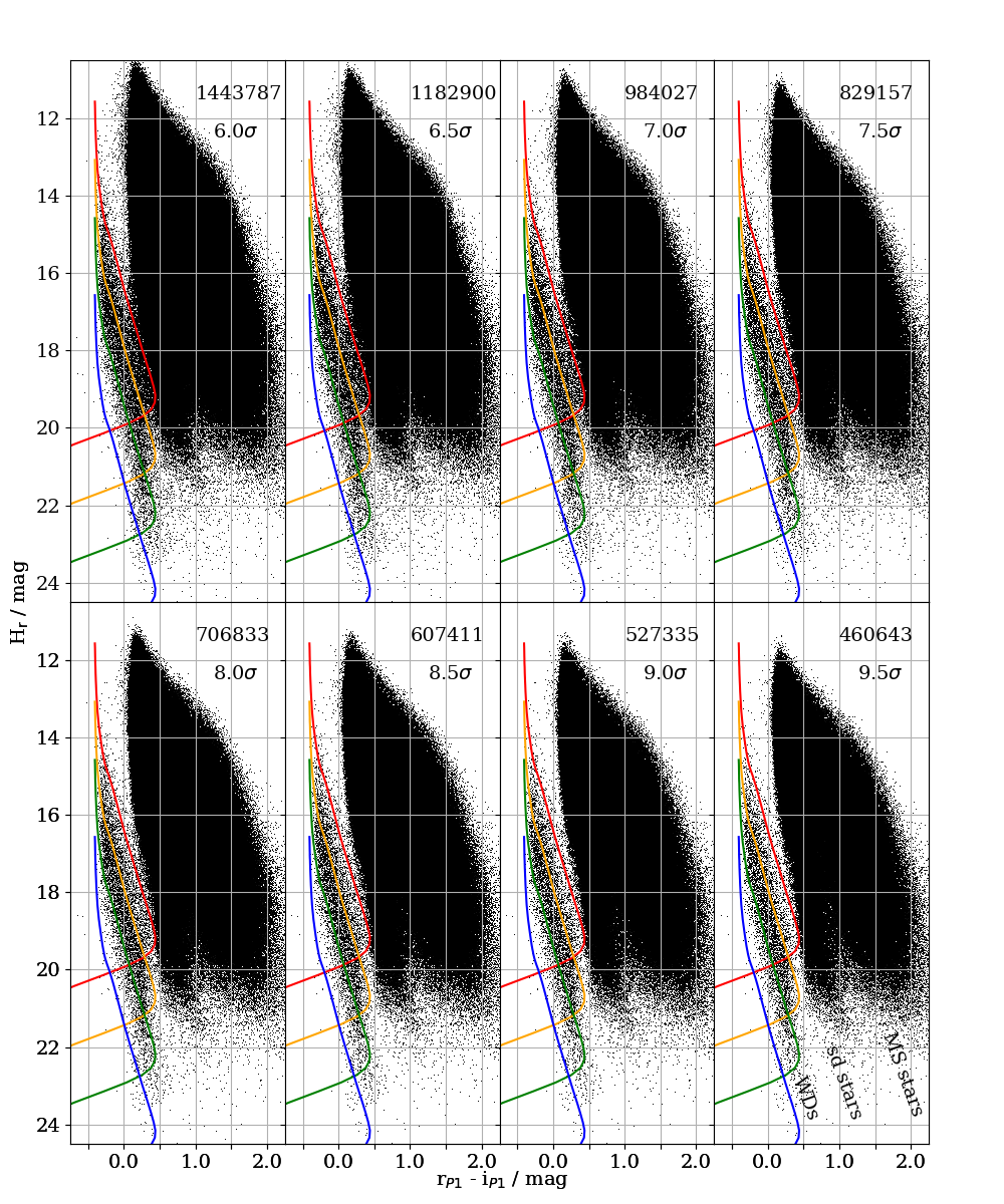
Figure 1: RPM diagrams with $\mu>5.0$ to $9.5\sigma$ from top left to bottom right. The numbers above the significance shows the total number of objects in the scattered plots. The red, yellow, green and blue lines are the cooling sequence for DA WDs with tangential velocity at $20,40,80$ and $200\mathop{}\!\,\mathrm{km\,s}^{-1}$. Most contaminants appear as vertical scatter with neutral colour ($0.0<$r${}_{\mathrm{P}1}-$i${}_{\mathrm{P}1}<0.5$).

2.3 Lower Proper Motion Limits

In order to select a clean sample of proper motion objects, we require our samples to have high S/N ratio in the proper motions. This excludes most of the non-moving objects from our catalogue and limits scatter in the RPM diagram. The total proper motion uncertainty of an individual object is given by

$$\sigma_{\mu}=\sqrt{\left(\frac{\mu_{\alpha}\cos(\delta)}{\mu}\right)^{2}\sigma_{\mu_{\alpha}\cos(\delta)}^{2}+\left(\frac{\mu_{\delta}}{\mu}\right)^{2}\sigma_{\mu_{\delta}}^{2}},$$ (5)

where $\mu$ is the total proper motion.

When $\sigma_{\mu}$ is plotted against r_P1 there is significant scatter at a given magnitude. However, a well defined relation between the proper motion uncertainty and magnitude is needed for volume integration and completeness corrections (Section 4.3). See Section 4.6 for how the individual lower proper motion limits can be applied to a sample from a non-uniform survey.

2.4 Upper Proper Motion Limit

The upper proper motion limit is determined by PS1 PV2 matching radius, matching algorithm and its efficiency.

Matching Radius

The search radius for cross-matching between different epochs of PS1 data was $1\arcsec\,yr^{-1}$. Although each part of the sky was imaged twelve times per year on average, some parts of the sky were limited by seasonal observability and weather. At low declinations, the sky could only be observed in a window of a few months every year so the maximum proper motion an object can carry is limited to roughly the size of the search radius per year, which is $1\arcsec\,yr^{-1}$.

Matching Algorithm

In PV2 high proper motion objects moving by more than $1\arcsec$ throughout the survey period would be detected as 2 or more separate objects. The IPP solves for the 5-parameter astrometric solutions that include parallax. In order to break the degeneracy in the parallax and proper motion in the astrometric solution, a minimum epoch difference of 1.5 years is required. For objects that move faster than $0.66\arcsec\,yr^{-1}$, they would have moved outside the matching radius after 1.5 years. Otherwise, these objects would have either erroneously large proper motion with small parallax or vice versa. Although it is possible to “stitch” the multiple parts back together and recalculate the proper motions with the maximal use of data, this creates a completeness problem to the faint high proper motion objects. When objects close to the detection limits can only be observed under the best observing conditions, there are not enough epochs to solve for the astrometric solution when they are split into parts. For example, if an object has 10 evenly distributed measurements that are catalogued as “2 sources” each with 5 measurements, the individual uncertainty would become $2\times\sqrt{2}\approx 2.28$ times larger than that is solved as a single object where the $2$ comes from the ratio of the maximum epoch difference and $\sqrt{2}$ comes from the ratio of the number of epochs.

Matching Efficiency

The high proper motion population is in the immediate solar neighbourhood so the number density is uniform at this limit. Through using proper motion as a proxy-parallax (like that in reduced proper motion), the number density follows

$$\log{N}\propto-3\log(\mu)$$ (6)

for a complete sample. In the 3$\pi$ Survey, the gradient deviates from $-2.7$ at $0.501\arcsec\,yr^{-1}$ (See Fig. 2).

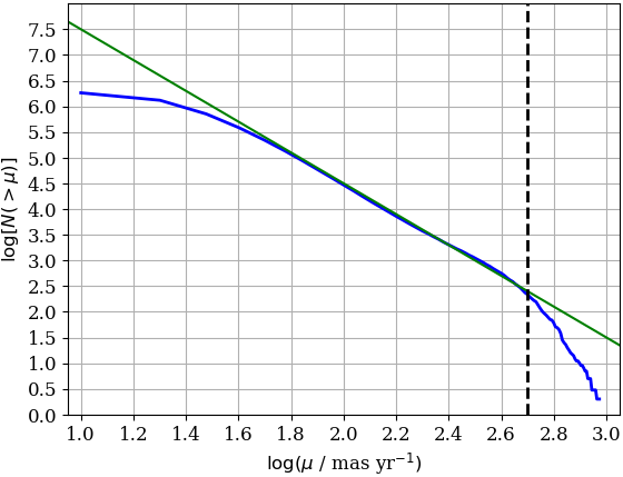
Figure 2: The logarithm of the number of object with proper motion larger than the given proper motion is plotted against proper motion (blue). Due to the small distances the high proper motion objects are at, the relation has a gradient of $-3$ as shown by the green line. Above $10^{2.7}=501\,\mathrm{mas}\,\mathrm{yr}^{-1}$ (dashed line), the underestimation of the number of objects implies an incomplete matching of those high proper motion objects

Combining the three cases, the matching efficiency gives the tightest limit among all, so the global upper proper motion limit in this study is set at $0.501\arcsec\,yr^{-1}$.

2.5 Faint Magnitude Limit

In order to find the faint magnitude limits at which data are complete, the object counts were compared against synthetic star and galaxy counts in g_P1, r_P1, i_P1 and z_P1 filters in 15 fields at high galactic latitudes to avoid interstellar extinction complicating this analysis. We chose a field of view of $\sim$$3.4$ square degrees (a HEALPix pixel size with $\mathrm{N}_{\mathrm{side}}=32$, see later), a size that is large enough for sufficient star counts and to smooth out inhomogeneity of galaxies while at the same time small enough to limit variations in data quality across the field (see Fig. 3). Each of the filter is treated independently in this exercise where each source is required to be detected at least 3 times with a magnitude uncertainty less than $0.2\mathop{}\!\,\mathrm{mag}$.

Stars

Differential star counts along the line of sight to each field were obtained using the Besançon Galaxy model (Robin et al., 2003, 2004). This employs a population synthesis approach to produce a self-consistent model of the Galactic stellar populations, which can be “observed” to obtain the theoretical star counts. It is a useful tool to test various Galactic structure and formation scenarios although we have adopted all the default input physical parameters except the latest spectral type is DA9 instead of the default DA5. There are only two photometric systems available, the Johnson-Cousins and the CFHTLS-Megacam systems. Since there is only a small difference between the PS1 and Megacam, the g’, r’, i’ and z’ are used to approximate the g_P1, r_P1, i_P1 and z_P1 in this work. The faint magnitude limits of the model are set at $25\mathop{}\!\,\mathrm{mag}$ to guarantee that the model is always complete as compared to the data.

Galaxies

Fainter than $\sim$$19\mathop{}\!\,\mathrm{mag}$, galaxies become unresolved (i.e., point-like) and have photometric parameters that overlap with stars. Therefore, it is necessary to include galaxies in the synthetic number counts. Galaxy counts to faint magnitudes have been determined in many independent studies. The Durham Cosmology Group has combined their own results (see e.g., Jones et al., 1991; Metcalfe et al., 1991) with many other authors. These are available online along with transformations to different photometric bands. They are provided in terms of log-number counts per square degree per half-magnitude unless specified otherwise. A cubic spline was fitted over all available observations to obtain the galaxy counts as functions of magnitude in each band.

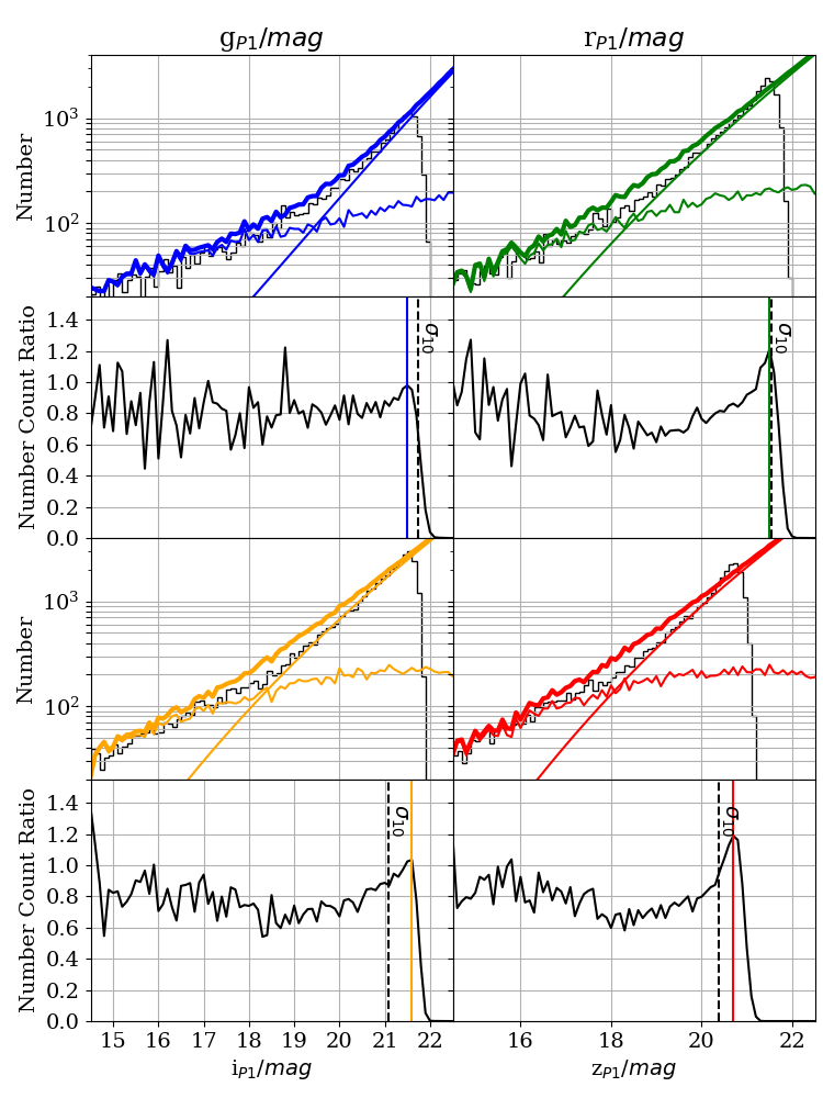
Figure 3: An example star and galaxy counts in g_P1 (purple), r_P1 (blue), i_P1 (green) and z_P1 (yellow) filters in the direction $(\alpha,\delta)=(0.0,-13.248015)$. The odd rows (from top) show the star and galaxy counts with thin colour lines and the combined star and galaxy counts in thick colour line. The black lines are the observed number counts. The even rows show the ratios between the model and observation, the dashed lines show the 10$\sigma$ photometric limits and the colour lines mark the completeness limit (see Section 2.6).

PS1 has a very complex variation in the data quality as a function of position. If the small/medium scale variations in the survey depth are not considered, the survey volume would be limited to the shallowest parts of the sky, which would be more than a magnitude brighter than the deepest parts. In order to take into account these small scale effects, a linear relationship between the completeness magnitude and the detection depth map (Farrow et al., 2014), $D(\alpha,\delta)$, was found empirically, see Fig. 4. Since the given depth maps are the $10\sigma$ detection limit in a fiducial $3\arcsec$ aperture we converted to FWHM magnitude by accounting for the flux included in the PSF, so the limiting magnitude was corrected with a linear transformation $D^{\prime}=D-2.5\times\log(2)$. The characteristics in the y_P1 band were assumed similar to the other filters.

2.6 Survey Depth

The $3.4$ square degrees field-of-view of PS1 is not small compared to the size of inhomogeneities in survey quality so there is some scatter in the completeness-depth relation. In order to account for these variations, instead of choosing the best fit straight line ($C$, where $C=0.6826\times\sigma_{10}+6.8197$), which has half the data points above the line and the other half below it, a straight line that would have covered 99.9% of all data was used, this corresponds to $3.090\,\sigma_{\mathrm{measured}}$. This threshold means that $99.9\%$ of the time the HEALPix pixel is complete. The scatter of these points was measured from the median absolute deviation (MAD) to minimize the effect from outliers, where $\sigma_{\mathrm{measured}}=1.48\times\mathrm{MAD}$. The completeness limit is

$$C^{\prime}=C-3.090\times\sigma$$ (7)

where $\sigma$ is measured to be $0.1359$.

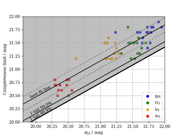
Figure 4: The completeness limits are plotted against the $10\sigma$ point source detection limits. The solid line is the best fit linear relation, dashed line is the vertical offset of the best fit solution that has covered $68.2\%$ of all data (i.e., $1\sigma$ in each direction).

By applying this relation to the photometric depth maps, the completeness maps in the five PS1 filters were produced. The resolution at which these maps were applied was degraded to $\mathrm{N}_{\mathrm{side}}=16$ to match the resolution of the tangential velocity completeness correction.

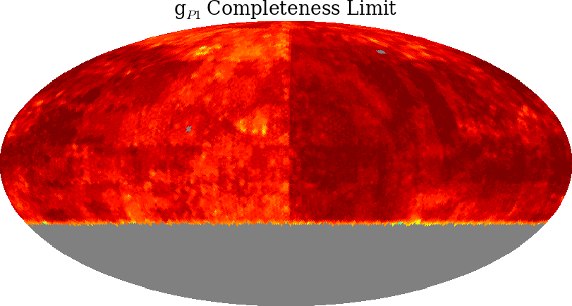
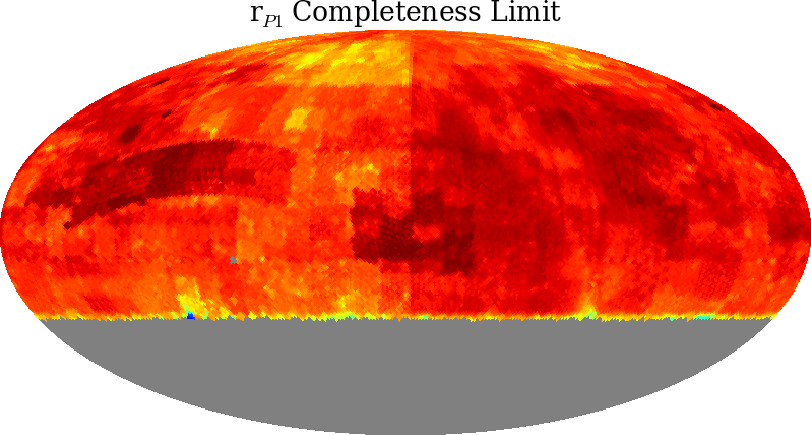
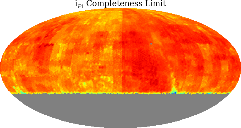
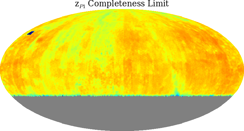
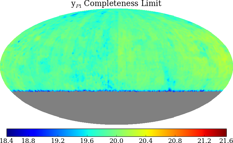
Figure 5: Completeness map in g_P1, r_P1, i_P1, z_P1 and y_P1 filters respectively, all magnitudes are with the same colour scale.

2.7 Bright Magnitude Limit

Brighter than $15\mathop{}\!\,\mathrm{mag}$, there is an astrometric bias that is colloquially known as the ‘Koppenhofer effect’ amongst the PS1 Science Consortium. The essence of the effect was that a large charge packet could be drawn prematurely over an intervening negative serial phase into the summing well, and this leakage was proportionately worse for brighter stars. The brighter the star, the more the charge packet was pushed ahead. The amplitude of the effect was at most $0.25^{\prime\prime}$, corresponding to a shift of about one pixel. Roughly a quarter of the data were affected before the problem was corrected (Magnier et al., 2016c). Since there are few WDs brighter than $15\mathop{}\!\,\mathrm{mag}$, we choose this as our bright limit to minimise the effect.

2.8 Object Morphology

All objects marked as good were selected (i.e., not flagged as extended, rock, ghost, trail, bleed, cosmic ray or asteroid).

Star-Galaxy Separation

The 3$\pi$ Survey catalogue has a star-galaxy separator (SGS) entry for every object. The typical photometric limits are $\sim$$21\mathop{}\!\,\mathrm{mag}$ in the optical and a typical FWHM of $1.2\arcsec$ so at the faint end of the survey, the realiability of the SGS is limited to the observing conditions. Therefore, we compared the SGS with the object classifier from the Canada-France-Hawai’i Telescope Lensing Survey (CFHTLenS, Heymans et al., 2012; Erben & CFHTLenS Collaboration, 2012 and Hildebrandt et al., 2012) employing codes CLASS_STAR, star_flag and FITCLASS. CFHTLenS is a $154$ square degrees multi-colour optical survey with the Megacam u*, g’, r’, i’ and z’ filters incorporating all data collected in the five-year period on the CFHT Legacy Survey, which was optimised for weak lensing analysis. The deep photometry in the i’-band was always taken in sub-arcsecond seeing conditions. Both star_flag and FITCLASS were optimised for galaxy selection, so the CLASS_STAR provided by SExtractor was used in this analysis. Considering the superior quality in both photometry and observing conditions of CFHTLS, at the limit of i${}_{\mathrm{P1}}\sim$$21\mathop{}\!\,\mathrm{mag}$, we assumed that CLASS_STAR was completely reliable. The pairing criteria of the two catalogues were $2^{\prime\prime}$ matching radius and $5\sigma$ proper motions.

In Fig. 6, the PS1 SGS is plotted against CLASS_STAR. We defined an object as a star when CLASS_STAR $>0.5$ or as a contaminant otherwise. The green dotted line indicates the PS1 SGS limit at $10.728$ which keeps the sample at $90.0\%$ complete and with a galaxy contamination rate of $3.9\%$.

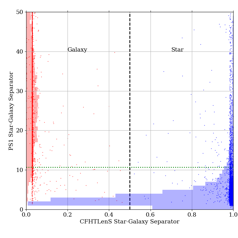
Figure 6: PS1 SGS is plotted against the CFHTLenS star galaxy separator, CLASS_STAR. When the CLASS_STAR is larger than $0.5$, it is considered as a star; otherwise, a galaxy. The green dotted line indicates the PS1 SGS limit. The semi-transparent histograms are the respective number counts as functions of PS1 SGS, the full range of the x-axis corresponds to a number count of $2,500$.

3 Selection Criteria - Derived Properties

The construction of a WDLF depends on the distance, luminosity and atmosphere type of the WDs, as well as the physical properties of the host population. Since most detected WDs lie within a few hundred parsecs from the Sun, the radial scale-lengths, which are of the order of kiloparsecs, of all Galactic components were not considered in this work. Interstellar reddening was corrected with the use of a three dimensional dust map when solving for the photometric parallax.

3.1 WD Atmosphere Type

On the theoretical front, WD atmospheres have been studied in detail. In recent years, with the abundant spectroscopic data available from SDSS, there were significant improvements in the understanding in the atmospheres. In addition to the conventional DA ($1,500$ K $<T_{\mathrm{eff}}<120,000$ K) models, synthetic photometry is available for 9 different hydrogen-helium mass ratios in the range $2,000$ K $<T_{\mathrm{eff}}<12,000$ K (Holberg & Bergeron, 2006; Kowalski & Saumon, 2006; Tremblay et al., 2011; and Bergeron et al., 2011). We choose the most helium rich model with $\log(\frac{\mathcal{M}_{\mathrm{He}}}{\mathcal{M}_{\mathrm{H}}}=8.0)$ to be our DB model. All models were provided in the PS1 filters by Dr. Pierre Bergeron (private communication). The cooling tracks of different chemical compositions are very similar above $T_{\mathrm{eff}}\sim 10,000$ K (i.e., $\mathrm{M}_{\mathrm{bol}}<12.0$).

3.2 Interstellar Reddening

A three dimensional map of interstellar dust reddening was produced using 800 million stars with PS1 photometry of which $200$ million also have 2MASS photometry (Green et al., 2015). Although there is a health warning that the reddening is “best determined by using the representative samples, rather than the best-fit relation”, with $\sim$$20,000$ spectroscopically confirmed WDs over the whole sky, most of which reside in the SDSS footprint, the only way to deredden our samples was to use the given best-fit solution. In order to convert the reddening values of $E(B-V)$ to extinction in the PS1 photometric systems, the values on Table 6 of Schlafly & Finkbeiner (2011) were used. We adopted the values from the column $R_{v}=3.1$ for this work (see Table 1).

Table 1: $A_{x}/E(B-V)_{SFD}$ in different passbands x, evaluated according to an Fitzpatrick (1999) reddening law with $R_{v}=3.1$ using a 7,000 K source spectrum. The subscript SFD refers to Schlegel et al. (1998).

Passband (x)	g	r	i	z	y
$A_{x}/E(B-V)_{SFD}$	3.172	2.271	1.682	1.322	1.087

The reddening information along the line of sight was given between distance modulus $4.0$ and $19.0$ in $0.5$ intervals. Each line of sight was interpolated with a cubic spline between the given points in order to compute the reddening at arbitrary distance.

3.3 Photometric Parallax

The surface gravities of WDs are narrowly distributed at about

$$\left<\log\,g\right>=7.937\pm 0.012$$ (8)

with SDSS DR10 (Kepler et al., 2015). Thus, by assuming a constant surface gravity at $\log(g)=8.0$, the distance and temperature of an object can be determined simultaneously. However, in doing so, extra scatter is introduced to the solution statistics. The goodness-of-fit $\chi^{2}_{\nu}$ would not be at $\sim$$1$. Therefore, a simple Monte Carlo method was used to produce a table of WDs following the distribution of equation 8. The standard deviations in magnitudes in each of the filters were found as a function of temperature for each of the DA and DB models ($\sigma_{log(g)}$). With these relations, it was possible to propagate the uncertainties arisen from adopting constant surface gravity into the final photometric parallax solutions (Fig. 7). This is also important in up/down-weighting different filters in the fitting procedure where the WD SEDs vary most significantly in the bluer filters.

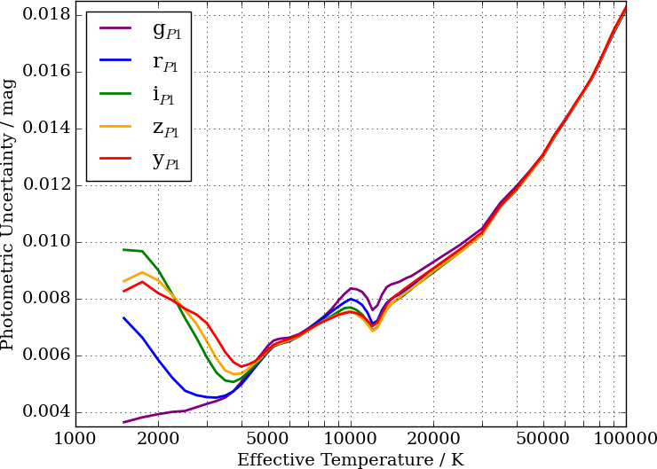
Figure 7: The standard deviations in magnitude in each filter when a population following the distribution described by equation 8 is assumed to have fixed surface gravity of $\log(g)=8.0$ for DA WDs.

The best-fit solutions with the DA and DB atmospheres were found by sampling the distance-temperature space with a Markov-Chain Monte-Carlo (MCMC) method emcee (Foreman-Mackey et al., 2013). In both cases, we used $20$ walkers of length $20,000$ with a burn-in phase of $1,000$ steps. There are some degeneracies in the solution, the most notable one being between a cool WD at small distance and a hot WD at large distance because interstellar reddening alters the shape of the model spectral energy distribution (SED). A simple minimisation technique (e.g., with Nelder-Mead method) sometimes cannot guarantee a global minimal in some cases.

When interstellar reddening is included in the calculation, the likelihood function to be maximised is

$$\sum_{i} \left\{\frac{\left[m_{i}-\mu_{D}-m_{\mathrm{model},i}(T_{\mathrm{eff}})-A_{i}(D)\right]^{2}}{\sigma_{i}^{2}+\sigma_{log(g),i}^{2}}+\right.$$ (9)

$$\hskip 14.22636pt\log\left[2\pi(\sigma_{i}^{2}+\sigma_{log(g),i}(T_{\mathrm{eff}})^{2})\right]\Bigg{\}}$$

where $m_{i}$ is the magnitude filter $i$, $\mu_{D}=5\log(D)-5$ is the distance modulus with subscript $D$ to distinguish it from the symbol for proper motion, $m_{\mathrm{model},i}(T_{\mathrm{eff}})$ is the magnitude of a given model which depends only on the effective temperature and $A_{i}(D)$ is the total extinction at distance $D$. In the case of the mixed atmosphere models, the model magnitude becomes $m_{\mathrm{model},i}(T_{\mathrm{eff}})$.

4 Survey Volume Maximisation

There are various statistical methods to arrive at a luminosity function. The most commonly used estimator in WD studies is the maximum volume density estimator (Schmidt, 1968). Its relatively straightforward approach has attributed to its popularity. This method was developed to combine several independent surveys (Avni & Bahcall, 1980) and to correct for scaleheight effects (Stobie et al., 1989; Tinney et al., 1993). Geijo et al. (2006) has shown that it is superior to the Chołoniewski and the Stepwise Maximum Likelihood method at the faint end of the WDLF, provided that the sample is sufficiently large, with more than $300$ objects. Like many previous works, when objects are both photometric and proper motion limited, extra caution is needed in order not to introduce bias. Simple, but sufficient at the time, assumptions were made to cope with such cases (Schmidt, 1975). However, it was shown in Lam et al., 2015  (hereafter LRH15) that the estimator underestimates the density of the intrinsically faint objects, and the modified maximum volume should be used where the discovery fraction is inseparable from the volume integrand. Lam (2017a, hereafter L17) further extended the LRH15 method to conduct object selection based on individual proper motion uncertainties before which a global uncertainty has to be used in order to perform completeness correction.

The maximum volume density estimator (Schmidt, 1968) tests the observability of a source by finding the maximum volume in which it can be observed by a survey (e.g., at a different part of the sky at a different distance). It is proven to be unbiased (Felten, 1976) and can easily combine multiple surveys (Avni & Bahcall, 1980). In a sample of proper motion sources, we need to consider both the photometric and astrometric properties (see LHR15 for details). The number density is found by summing the number of sources weighted by the inverse of the maximum volumes. For surveys with small variations in quality from field to field and from epoch to epoch, or with small survey footprint areas, the survey limits can be defined easily. However, in modern surveys, the variations are not small; this is especially true for ground-based observations. Therefore, properties have to be found locally to analyse the data most accurately. Through the use of Voronoi tessellation, sources can be partitioned into individual 2D cells within which we assume the sky properties are defined by the governing source. Each of these cells has a different area depending on the projected density of the population.

HEALPix is the acronym for Hierarchical Equal Area isoLatitude Pixelization of a sphere (Górski et al., 2005). This pixelisation routine produces a subdivision of a spherical surface in which all pixels at the same level in the hierarchy cover the same surface area. All pixel centres are placed on rings of constant latitude, and are equidistant in azimuth (on each ring). However, the pixels are not regular in shape. A HEALPix map has $\mathrm{N}_{\mathrm{pix}}=12\mathrm{N}_{\mathrm{side}}^{2}$ pixels each with the same area $\Omega=\pi/3\mathrm{N}_{\mathrm{side}}^{2}$, where $\mathrm{N}_{\mathrm{side}}$ is the square root of the number of division of the base pixel and it can be any value with a base of 2 (i.e., $2^{x}$ for any positive integer $x$). This pixelisation routine is used in computing the tangential velocity completeness correction.

In the rest of the article, cell will be used to denote Voronoi cell and h-pixel for HEALPix pixel.

4.1 Tangential Velocity Completeness Correction

In order to clean up the sample of proper motion objects, a lower tangential velocity limit was applied to remove spurious sources (low-velocity WDs have similar RPMs to those of high velocity subdwarfs from the Galactic halo). For example, $20,30$ or $40\mathop{}\!\,\mathrm{km\,s}^{-1}$ are typical choices to obtain clean samples of the disc populations, the precise choice of the value depends on the data quality; and $160,200$ or $240\mathop{}\!\,\mathrm{km\,s}^{-1}$ are used to obtain stellar halo objects (H06, RH11, M17). However, this process removes genuine objects from the sample. With some knowledge of the kinematics of the solar neighbourhood, it is possible to model the fractions of objects that are removed in any line of sight. A resolution of $\mathrm{N}_{\mathrm{side}}=16$ was used to pixelise the sky into $3,072$ h-pixels in order to account for the variation in the projected kinematics across the sky.

The problem of incompleteness as a result of kinematic selection bias was identified by Bahcall & Casertano (1986). A Monte–Carlo (MC) simulation was used to correct for such incompleteness by comparing with star counts. This correction, known as the discovery fraction, $\chi$, was then applied by H06. Instead of using a simulation, Digby et al. (2003) arrived at the discovery fractions by integrating over the Schwarzschild distribution functions to give the tangential velocity distribution, $\mathrm{P}(v_{\mathrm{T}},\alpha,\delta)$. This was done by projecting the velocity ellipsoid of the Galactic populations on to the tangent plane of observation, correcting for the mean motion relative to the Sun, and marginalising over the position angle to obtain the distribution in tangential velocity (see Murray, 1983). The values adopted for the mean reflex motions and velocity dispersion tensors are given in Table 2. These are obtained from the Fuchs et al. (2009) study of SDSS M dwarfs, with values taken from their 0–100 pc bin that is least affected by the problems associated with the deprojection of proper motions away from the plane (McMillan & Binney, 2009). RH11 further generalised the technique to cope with an all sky survey as opposed to the individual fields of view employed in earlier works. However, there are some discrepancies between the parameter space in which the volume and the discovery fractions were integrated over in all these cases. In order to generalise over a proper motion limited sample properly, the effects of the tangential velocity limits and the proper motion limits have to be considered simultaneously at each distance interval. The discovery fraction at a given distance, $\chi(\alpha_{h},\delta_{h},r)$, can be found from the normalised cumulative distribution function of the WD tangential velocity,

$$\chi(\alpha_{h},\delta_{h},r)=\int_{a(r)}^{b(r)}\mathrm{P}(v_{\mathrm{T}},\alpha_{h},\delta_{h})\mathrm{d}v_{\mathrm{T}}$$ (10)

where

$$a(r)=\mathrm{max}(v_{\mathrm{min}},4.74047\times\mu_{\mathrm{min}}\times r)$$ (11)

and

$$b(r)=\mathrm{min}(v_{\mathrm{max}},4.74047\times\mu_{\mathrm{max}}\times r),$$ (12)

where the subscript $h$ denotes the properties of a h-pixel; $v_{\mathrm{min}}$ and $v_{\mathrm{max}}$ are the minimum and maximum tangential velocity limit; the factor of $4.74047$ comes from the unit conversion from arcsec yr^-1 to km s^-1 at distance $r$ in unit of pc; $4.74047\mu_{\mathrm{min}}r$ and $4.74047\mu_{\mathrm{max}}r$ are the tangential velocity limits at distance $r$ arising from the proper motion limits. The appropriate limits on the integral are found by considering both of them.

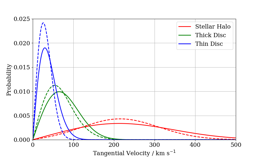
Figure 8: The tangential velocity distribution of the thin disc, thick disc and stellar halo in the direction of the North Galactic Pole (solid lines) and the Galactic Anti-Center (dashed line) based on the kinematic information from Table 2.

Table 2: Physical properties of the Galaxy used in the Schwarzschild distribution functions. The thick disc parameters are provided for illustration purpose only.

Parameter	Thin disc	Thick disc	Stellar Halo
$\langle$U$\rangle/\mathop{}\!\,\mathrm{km\,s}^{-1}$	-8.62a	-11.0c	-26.0c
$\langle$V$\rangle/\mathop{}\!\,\mathrm{km\,s}^{-1}$	-20.04a	-42.0c	-199.0c
$\langle$W$\rangle/\mathop{}\!\,\mathrm{km\,s}^{-1}$	-7.10a	-12.0c	-12.0c
$\sigma_{U}/\mathop{}\!\,\mathrm{km\,s}^{-1}$	32.4a	50.0c	141.0c
$\sigma_{V}/\mathop{}\!\,\mathrm{km\,s}^{-1}$	23.0a	56.0c	106.0c
$\sigma_{W}/\mathop{}\!\,\mathrm{km\,s}^{-1}$	18.1a	34.0c	94.0c
H/pc	250b	1000d	$\infty$

1. Fuchs et al. (2009)

2. Mendez & Guzman (1998)

3. Chiba & Beers (2000)

4. Girard et al. (2006)

4.2 Density Profile

Luminous WDs near the faint limits can be several hundred parsecs from the Galactic plane, where their space density is significantly reduced. In order to correct for the stellar density effect on the survey volume, the density scaling of the Galaxy has to be considered. Since the radial profile is large even when compared to the distance of the most luminous objects, only the scaleheight, which is perpendicular to the plane, was considered.

Thin Disc

The thin disc employs an exponential decay law to correct for the “reduction in survey volume” by the scaleheight effect. The density profile combined with all the appropriate correction becomes

$$\frac{\rho(r)}{\rho_{\odot}}=\exp\left(-\frac{|r\sin(b)+z_{\odot}|}{\mathrm{H}}\right)$$ (13)

where $|z|=r\sin{(b)}$ is the Galactic plane distance with $r$ being the line of sight distance, $b$ the Galactic latitude, the solar distance from the Galactic plane is $z_{\odot}\sim 20$ pc (Reed, 2006) and H the scaleheight.

Mendez & Guzman (1998) obtained a value of $\mathrm{H}_{\mathrm{thin}}=250$ pc based on faint main-sequence stars. These are likely of similar age to the WDs candidates in this work and are expected to show a similar spatial distribution and having been subjected to the same kinematic heating. This value is the most accepted value among works on WDLFs although there is evidence that the scale height for faint objects is larger (H06).

Stellar Halo

The scaleheight of the halo is of order of kiloparsecs. For the depth this work probed, the most distant objects are only a few hundred parsecs from the sun, it is valid to assume a uniform density profile.

4.3 Modified Volume Density Estimator

The modified volume density estimator (LRH15) is a variant of the maximum volume density estimator that is generalised over a proper motion limited sample. In order to calculate the volume available for the object, at each distance step of the integration both the stellar density profile and discovery fractions are considered. The total modified survey volume between r${}_{\text{min}}$ and r${}_{\text{max}}$ is therefore written as

$$\mathrm{V}_{\mathrm{mod}}=\Omega\int_{r_{\mathrm{min}}}^{r_{\mathrm{max}}}\frac{\rho(r)}{\rho_{\odot}}r^{2}\chi(\alpha,\delta,r)\mathrm{d}r,$$ (14)

where $\chi(\alpha,\delta,r)$ is from Equation 10 and the distance limits are solely determined by the photometric limits of the survey

$$r_{\mathrm{min}}=r\times\mathrm{max}\left[10^{\frac{1}{5}(m_{\mathrm{min},i}-M_{i})}\right]$$ (15)

and

$$r_{\mathrm{max}}=r\times\mathrm{min}\left[10^{\frac{1}{5}(m_{\mathrm{max},i}-M_{i})}\right].$$ (16)

The number density of a given magnitude bin is the sum of the inverse modified volume

$$\Phi_{k}=\sum_{i}^{N_{k}}\frac{1}{\textrm{V}_{\textrm{mod, i}}},$$ (17)

for N_k objects in the $k$-th bin. The uncertainty of each star’s contribution is assumed to follow Poisson statistics. The sum of all errors in quadrature within a luminosity bin is therefore written as

$$\sigma_{k}=\left[\sum_{i=1}^{N_{k}}\left(\frac{1}{\textrm{V}_{\textrm{mod}}}\right)^{2}\right]^{1/2}.$$ (18)

4.4 Voronoi Tessellation

A Voronoi tessellation is made by partitioning a plane with $n$ points into $n$ convex polygons such that each polygon contains one point. Any position in a given polygon (cell) is closer to its generating point than to any other points. For use in astronomy, such a tessellation has to be done on a spherical surface (two-sphere).

In this work, the tessellation is constructed with the SciPy package spatial.SphericalVoronoi, where each polygon is given a unique ID that is combined with the vertices to form a dictionary. The areas are calculated by first decomposing the polygons into spherical triangles with the generating points and their vertices (Reddy, 2015) and then by using L’Huilier’s Theorem to find the spherical excess. For a unit-sphere, the spherical excess is equal to the solid angle of the triangle. The sum of the constituent spherical triangles provides the solid angle of each cell. See Section 2 of L17 for detailed description.

4.5 Cell Properties

For a Voronoi cell $j$, the properties of the cell are assumed to be represented by generating source $i$. Both $i$ and $j$ are indexed from $1$ to $\mathcal{N}$, but since each source has to be tested for observability in each cell to calculate the maximum volume, $i$ and $j$ cannot be contracted to a single index. Furthermore, the cells do not need to be defined by only the sources of interest. Arbitrary points can be used for tessellation such that $i$ and $j$ will not have a one-to-one mapping. The epoch of the measurement is labelled by $k$. In this work, we use the full catalogue with $14,598$ sources to generate the Voronoi tessellation, and analysis were performed using this fixed set of cells (See Table 3 for the catalogue of these sources, and Table 4 for the epoch information).

4.6 Voronoi V_max

In order to incorporate the Voronoi tessellation into the modified volume method, two minor adjustments are required to apply to the volume integral – (1) the lower proper motion limit; and (2) the area element $\Omega_{j}$ in Equation 19.

Lower Proper Motion Limit

$$\mathrm{V}_{\mathrm{max}}=\sum_{j}\Omega_{j}\int_{r_{\mathrm{min,j}}}^{r_{\mathrm{max,j}}}\dfrac{\rho(r)}{\rho_{\odot}}\times r^{2}\\ \hfill\times\left[\int_{a(r)}^{b(r)}P_{h(j)}(v_{\mathrm{T}})\,\mathrm{d}v_{\mathrm{T}}\right]\mathrm{d}r$$ (19)

where $\dfrac{\rho(r)}{\rho_{\odot}}$ is the density normalized by that at the solar neighbourhood, $P_{h(j)}$ is the tangential velocity distribution, $h(j)$ denotes the h-pixel mapped from cell $j$ with area $\Omega_{j}$, $v_{\mathrm{T}}$ is the tangential velocity, $r_{\mathrm{min}}$ and $r_{\mathrm{max}}$ are the minimum and maximum photometric distances, and $\sigma_{\mu}(r)$ is the proper motion uncertainty as a function of the distance to the source. Consequentially, at each step of the integration, the $\sigma_{\mu}$ has to be recomputed (L17, necessary epoch informations can be found in 4). With a set of catalogued observational data, new interstellar reddening has to be applied at the new distance before the “new observed flux” is converted into instrumental flux by using the given zero-points. A set of new photometric and astrometric uncertainties can then be recomputed based on the instrumental flux, epoch sky brightness, dark current and read noise. The uncertainties are checked against the desired limits in order to identify the distance limit for the volume integration. The lower tangential velocity limit in the inner integral, $a(r)$, is

$$a(r)=\mathrm{max}\left[v_{\mathrm{min}},4.74047\times s\times\sigma_{\mu}(r)\times r\right]$$ (20)

where $v_{\mathrm{min}}$ is the global lower tangential velocity limit and $s$ is the significance of the proper motions, which is $7.5$ in this work.

4.6.1 Voronoi Cell Area

In the framework of L17, the simulated data is an all sky survey with no spatial selection criteria. However, in any given survey or analysis, there are usually spatial limits (e.g., selection or limits on right ascension and declination; or leaving out dense regions to avoid confusion). When such selections are necessary, since the Voronoi cells constructed with the data always cover the entire sphere (i.e., the total solid angle is $4\pi$), it is necessary to add artificial points to the set of data in order to define the set of Voronoi cells that carry the appropriate areas. In order to align the artificial cells boundaries with the selection borders, tightly spaced points along two rings at equidistance from the border are required. In this work, we add $21,600$ points on each ring which would be equivalent to a spacing of $1\arcmin$ at the equator. The spacing between the ring and the border is $3\arcsec$. By identifying where the artificial points belong in the original Voronoi cells (hereafter the bounding cells), the areas of the Voronoi cells generated from the respective artificial points are added to the new areas of the bounding cells (see Fig. 9). It is trivial to add points along a single coordinate axis. However, when the area within the $20\degr$ radius from the galactic centre is removed from our survey, the positions that trace two rings on either side at eqidistance from the selection boundary are not trivial to calculate. It is much simpler to define a dummy coordinate system such that the Galactic Centre is located at the Pole. In such configuration, the rings can be defined by a single coordinate axis. This can be done by rotating the Galactic Coordinates by $90\degr$ along the vector joining the centre of the celestial sphere to $(l,b)=(90,0)$. We use the Euler-Rodrigues formula for this purpose.

There is one caveat, the lines joining the Voronoi vertices are great circle lines. However, many selections, for example lines of equal-declination, are traced by small circles, so the area of any Voronoi cells constructed this way are only approximations, but they are only offsets by negligible amounts.

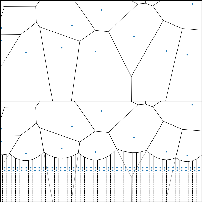
Figure 9: Top: A simple illustration of Voronoi cells at the survey boundaries. Bottom: Voronoi cells after artificial points added. Grey lines shows the original cell boundaries. The areas generated from the artificial points are added to the host cell, which is approximated by assigning the artificial points to the host cell. In the observed sample, the number ratio between the cells containing a genuine object and the artificial cells is much larger than it is shown here for illustration purpose.

4.7 Interstellar reddening

Interstellar reddening has small effect in determining the distance and bolometric magnitude of an individual object. However, it causes a change in the shape of a WDLF when a large sample is considered. When WDs cool down, they turn red until they reach $\sim$$6,000$ K beyond which they start to turn blue due to H2CIA. Therefore, the hot and cool WDs require larger corrections than the warm ones. Without extinction correction, the bright end of the WDLF will have a larger gradient (more positive), while the faint end will have a smaller (more negative) gradient. In order to correct for the interstellar reddening, Equations 15 and 16 have to be modified to

$$r_{\mathrm{min}}=r\times\mathrm{max}\left[10^{\frac{1}{5}(m_{\mathrm{min},i}-M_{i}-A_{i}(r)+A_{i}(r_{\mathrm{min}}))}\right]$$ (21)

and

$$r_{\mathrm{max}}=r\times\mathrm{min}\left[10^{\frac{1}{5}(m_{\mathrm{max},i}-M_{i}-A_{i}(r)+A_{i}(r_{\mathrm{max}}))}\right].$$ (22)

5 White Dwarf Luminosity Functions

In addition to applying all the selection criteria discussed in Section 2, finder charts were inspected to remove spurious objects. The survey contains $14,598$ WD candidates with $v_{\textrm{tan}}>40\mathop{}\!\,\mathrm{km\,s}^{-1}$ and proper motion at $7.5\sigma$ significance. However, a proportion of them do not enter any of the analysis due to the stringent velocity and photometric parallax quality selection in deriving WDLFs that are representative of the disc (low velocity sample) and halo (high velocity sample).

5.1 WDLFs combining two Atmosphere Models

To limit contaminations, the maximum goodness-of-fit reduced chi-squared of the photometric parallax ($\chi^{2}_{\mu}$) is set at $10$ above $6000$ K and at $2$ below that. The smaller tolerance comes from the “blue hook” of the WD cooling sequence where spurious objects (e.g., high proper motion subdwarfs) are much more likely to be fitted as WDs. The mixed hydrogen-helium atmosphere model is only available below $12,000$ K ($\sim$$11.5\mathop{}\!\,\mathrm{mag}$). Above this there is little difference in the models and only DA is considered in constructing the luminosity function. Because of the lack of available DB models above $12,000$ K, objects in the range of $10,000-12,000$ K tend to have poor goodness-of-fit. To avoid this systematic bias, objects are divided into $3$ groups where the latter 2 are summed with appropriate weightings to give the total WDLFs :

• Objects with best fit DA temperature above $10,000$ K;

• Objects with best fit DA temperature below $10,000$ K and have good DA fit;

• Objects with best fit DA temperature below $10,000$ K and have good DB fit.

Objects in (i) is unit-weighted; for those in (ii) and (iii), they are weighted by the using the reduced chi-squared value, $\chi^{2}_{\mu}$, of the photometric parallax. The probability of an object being a DA and DB are $P_{\mathcal{A}}\propto\exp(-0.5\chi^{2}_{\mu,\mathcal{A}})$ and $P_{\mathcal{B}}\propto\exp(-0.5\chi^{2}_{\mu,\mathcal{B}})$ respectively. The weights of objects being DA and DB are the ratio of the two probabilities. The total luminosity function is the weighted sum of the inverse maximum volume.

5.2 WDLF of the Low Velocity Sample in the Solar Neighbourhood

The WDLFs of the low velocity sample (hereafter, disc), are shown in Fig. 10. In the $40-60$ and $40-80\mathop{}\!\,\mathrm{km\,s}^{-1}$ samples, there are $6,495$ and $9,561$ WD candidates and the integrated WD densities are $5.314\pm 0.487\times 10^{-3}$ and $5.657\pm 0.416\times 10^{-3}$ pc^-3 respectively, where the corresponding $\left\langle\mathrm{V}/\mathrm{V}_{\mathrm{max}}\right\rangle$s are $0.547\pm 0.004$ and $0.556\pm 0.003$. Since the cooling time for DA with $\log(g)=8.0$ to reach $16.0$, $16.5$, $17.0$, $17.5$ and $18.0$ mag are $9.36$, $10.39$, $11.16$, $11.84$ and $12.49\mathop{}\!\,\mathrm{Gyr}$ respectively, and $8.61$, $9.46$, $10.27$, $11.07$ and $11.88\mathop{}\!\,\mathrm{Gyr}$ for DB; the faintest objects are most likely coming from the low velocity tail of the thick disc kinematic distribution. An alternative explanation is that they are low mass WD that have a higher cooling rate and lower surface gravity: at $\log(g)=7.0$, the cooling ages for DA drop to $3.44$, $4.24$, $6.33$, $9.02$ and $11.62\mathop{}\!\,\mathrm{Gyr}$. However, this is inconsistent with the assumption of a fixed surface gravity $\log(g)=8.0$ in our analysis. In the $25$ pc volume limited sample from Holberg et al. (2016), at the $17.5\mathop{}\!\,\mathrm{mag}$ bin, there are a massive DB, with $\log(g)=9.0$, belonging to a widely separated double degenerate system and a DA presumed to have $\log(g)=8.0$. SED fitting with 5-band broadband photometry cannot reliably fit the surface gravity or surface hydrogen/helium ratio as free parameters. It will only be possible for a large sky area survey to expand the fitting parameter space with, for example, the future Gaia data release where parallax and low resolution spectra would be available for most of the nearby sources.

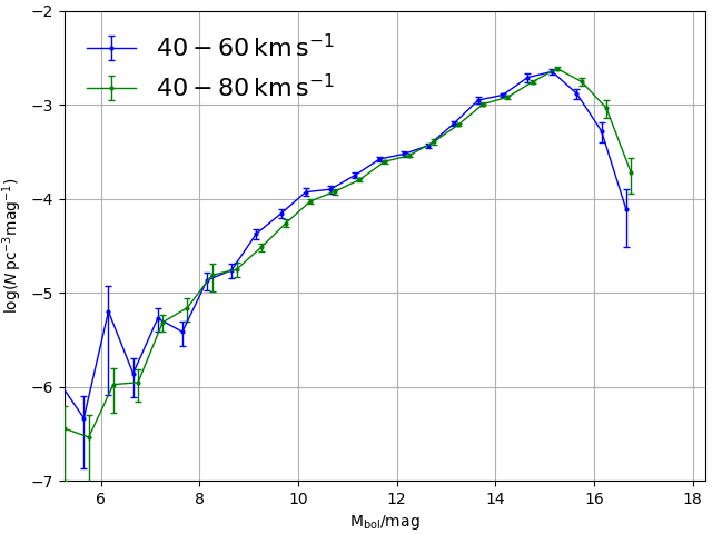
Figure 10: WDLF of the low velocity samples in the solar neighbourhood. The $40-80\mathop{}\!\,\mathrm{km\,s}^{-1}$ line is shifted by $0.1\mathop{}\!\,\mathrm{mag}$ for easier visual comparison. The two samples agree well with each other.

The smaller the range of tangential velocities, the fewer contaminants from the disc main sequence stars. However, the WDLF would become more model dependent on the Galactic model and more sensitive to the completeness corrections.

5.3 WDLF of the High Velocity Sample in the Solar Neighbourhood

The high velocity samples contain $1.334\pm 0.420\times 10^{-4}$, $1.798\pm 1.487\times 10^{-4}$, $5.291\pm 2.717\times 10^{-5}$, $1.006\pm 0.950\times 10^{-4}$ and $3.296\pm 2.849\times 10^{-5}$ pc^-3 for the tangential velocity selection between $160$, $180$, $200$, $220$ & $240\mathop{}\!\,\mathrm{km\,s}^{-1}$ and $500\mathop{}\!\,\mathrm{km\,s}^{-1}$. The five samples have $\left\langle\mathrm{V}/\mathrm{V}_{\mathrm{max}}\right\rangle$ at $0.427\pm 0.016$, $0.447\pm 0.020$, $0.459\pm 0.024$, $0.434\pm 0.031$ and $0.432\pm 0.039$. The decrease in the number density comes from the lack of the faintest candidates in the higher velocity samples; the five WDLFs agree with each other at the brighter end is a good indication that the samples are properly normalized (Fig. 11). The $160$ & $180\mathop{}\!\,\mathrm{km\,s}^{-1}$ samples are contaminated by a non-negligible amount of thick disc WDs, the faintest bins in the $160\mathop{}\!\,\mathrm{km\,s}^{-1}$ sample are most likely coming from the disc. The $200\mathop{}\!\,\mathrm{km\,s}^{-1}$ sample should be the lowest reliable tangential velocity cut for testing the sample as from a halo population (RH11, M17). However, one has to be cautious when selecting sub sample as halo candidates as it is very likely we are looking at the tail of the thick disc distribution (Oppenheimer et al., 2001; Reid et al., 2001). It appears that the down turn of the halo WDLF is still out of reach of Pan–STARRS 1.

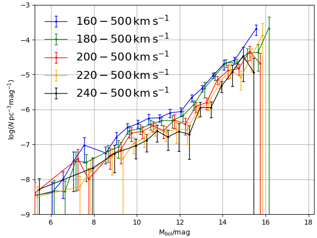
Figure 11: WDLF of the high velocity sample in the solar neighbourhood. The WDLF with a selection of $200-500\mathop{}\!\,\mathrm{km\,s}^{-1}$ is located at the correct magnitude. Each successive decrement and increment in the lower tangential velocity limit shifts the WDLFs by $-0.1\mathop{}\!\,\mathrm{mag}$ and $+0.1\mathop{}\!\,\mathrm{mag}$ respectively for easier visual comparison. All WDLFs agree well with each other up to $15.25\mathop{}\!\,\mathrm{mag}$ when the larger lower-tangential velocity limit removes the faintest objects.

5.4 Data available online

Machine readable text files are available online as supplementary materials to generate Figure 10 and 11. See Table 5 for the description.

6 Comparison with Previous Works

There are three works on WDLFs in the past $20$ years employing large sky area photometric surveys: the H06, RH11 and M17. The former two rely on photographic plates so they are much more limited by the astrometry in the faint end. In M17, the combination of SDSS, the Bok $90$-inch telescope at the Steward Observatory and the $1.3$ m telescope at Flagstaff Station, USNO has enabled unprecedented photometric and astrometric quality for work on WDLF to date. Its strengths are both the low proper motion uncertainty and survey depth; in comparison, 3$\pi$ Survey strength is the rapid re-imaging and the full visible sky at Haleakal$\bar{\mathrm{a}}$ which gives a footprint area $11.4$ times larger than that in M17. We believe the M17 WDLFs should be considered as the best reference available at this moment. However, when drawing comparisons, it is unclear whether it has probed sufficiently far away that the study has reached some local Galactic structures of over- or under-density.

6.1 Low Velocity Sample/disc(s)

As shown in Fig. 12, our WDLF has the same general shape compared to the past works, which is expected as it takes a significantly different Galactic density profile or star formation history in order for the shape to vary noticeably. This work has very similar density to all previous works, despite the use of a new generalized maximum volume method. We note that H06 and M17 have similar footprints; and the footprint in this work is similar to that in RH11. The density differences in local Galactic structures or an evolving scaleheight, instead of a fixed $250$ pc, may attribute to some of the discrepancies. From H06, it is understood that a fixed scaleheight is not the most appropriate assumption in studying the disc sample: fainter populations follow larger scaleheights, due to kinematic heating of the discs. The smaller footprint area and less coverage near the Galactic plane in H06 and M17 means that the variations in density is likely to be smaller. The large footprint area at greater depth in this work as compared to RH11 could have amplified the effect. In the $4$ works shown in Fig. 12, we suspect that H06, with the smallest sample volume, is displaying the feature at the bright end of the WDLF that was understood as an enhanced star formation from the $25$ pc sample Holberg et al. (2016). While in the M17, which is essentially a deeper version of H06, such enhanced density is not shown; in RH11 and this work, the footprint areas are a few times larger, small scale (hundreds of squared degrees) features are likely to be averaged out. The different atmosphere models adopted by the four works can also contribute to the discrepancies. The bumps at $\sim$$10$ and $\sim$$12\mathop{}\!\,\mathrm{mag}$ appear in all $4$ works is evidence that they are genuine features of recent star burst ($\sim$$1\mathop{}\!\,\mathrm{Gyr}$). This feature is more prominent for a more stringent volume-limited sample (Oswalt et al., 2017). The precise time of the star burst can only be revealed by a proper SFH analysis. The integrated number density $5.657\pm 0.416\times 10^{-3}$ pc^-3 of this work is in very good agreement with the $5.5\pm 0.1\times 10^{-3}$ pc^-3 from M17; and the $4.6\pm 0.5\times 10^{-3}$ pc^-3 by H06.

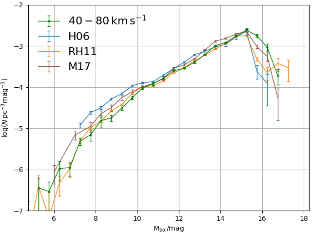
Figure 12: Comparison of WDLFs of the low velocity sample in H06, RH11, M17 and this work. This work is reporting a similar integrated number density to all previous works.

6.2 High Velocity Sample/Halo

The WDLF ($200-500\mathop{}\!\,\mathrm{km\,s}^{-1}$) of the high velocity sample agrees well with previous works (Fig. 13). The integrated density at $5.291\pm 2.717\times 10^{-5}$ pc^-3 is slightly higher than $4.0\times 10^{-5}$ pc^-3 and $3.5\pm 0.7\times 10^{-5}$ pc^-3 by H06 and M17 respectively, but they are within $1\sigma$ confidence limit from each other; and it is well under $1.9\times 10^{-4}$ pc^-3 reported by the effective volume method (RH11). The disc-to-halo ratio in this work is $107$, which is about $30\%$ smaller than the $157$ found in M17; very similar to H06’s value at $115$. The most appropriate comparison from RH11 is the ratio between the sum of the densities of the discs and that of the halo found from the effective volume methods, at $19.7$. However, it is worth noting the different faint limits each WDLF probes, the lack of data in the highest density bin, which is most likely in the range $16-18\mathop{}\!\,\mathrm{mag}$, bias the disc-to-halo ratio significantly.

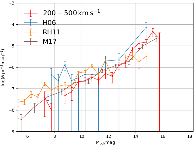
Figure 13: Comparisons of WDLFs of the high velocity sample in H06, RH11, M17 and this work. This work has a lower density in the range of $8-13\mathop{}\!\,\mathrm{mag}$, but it still agrees to within $1\sigma$ combined uncertainties. The integrated number densities are all within $1\sigma$ confidence from each other, except for RH11.

6.3 Data available online

Machine readable text files are available online as supplementary materials to generate Figure 12 and 13. See Table 6 for the description.

7 Summary and Future Work

We have applied the newest V_max method from L17, which formally propagates instrumental noise from individual epoch to proper motions uncertainties, to derive the disc and halo WDLFs from the Pan–STARRS 1 3$\pi$ Survey. The number densities are found to be $5.657\pm 0.416\times 10^{-3}$ pc^-3 and $5.291\pm 2.717\times 10^{-5}$ pc^-3 respectively. Both results are consistent with previous results from studies of a similar kind.

In order to study the Galactic components independently, a rigorous statistical method has to be devised (e.g., extending on RH11, Lam 2017b) in order to derive the star formation history of the individual components through the inversion of the respective WDLFs. The WD candidates from the Gaia DR2 selected by parallax (e.g., Hollands et al. 2018; Gentile Fusillo et al. 2018) as opposed to by proper motion and the subsequent releases will provide an order of magnitude more WDs with full 5 astrometric solutions and low resolution spectra (DR3+) will potentially shed new light to the understanding of this, currently, elusive population; better understanding to the kinematics and density profiles can derive more accurate WDLFs. In the subsequent work, we will apply a similar selection and analysis on the Gaia data, which will show the definite solution in the next couple of decades. It is the dawn of WD science in this coming era with multiple large sky area photometric and spectrometric surveys coming online.

Appendix A Supplementary Materials

The following tables describe the content of the supplementary material available online. In Table 3 and 4, the joint Catalogue ID and Object ID form an unique ID to map the epoch measurements to the source. However, this is not an unique ID over different processing versions and data releases. There are not direct mappings between the sources in this catalogue (PV2) and the public releases DR1 and DR2. Table 4 is divided into two compressed files, first one contains all measurements with R.A. between $0\degr$ and $180\degr$; and the second one with $180\degr$ to $360\degr$.

Table 3: Description of the full catalogue used to generate the Voronoi Tessellation containing $14,598$ sources. A number of these sources were only used to model the survey properties but were not directly used in computing the WDLFs. See Section 5 for the selection criteria for the various WDLFs. The joint Catalogue ID and Object ID forms an unique ID, however, this is not unique over different processing versions and data releases.

Column	Description
1	Right Ascension (epoch at the Mean Epoch and equinox at 2000.0)
2	Declination (epoch at the Mean Epoch and equinox at 2000.0)
3	Catalogue ID
4	Object ID
5	Mean Epoch (number of seconds since 1 January 1970)
6	Original Proper Motion in the direction of R.A. $(^{\prime\prime}\,\mathrm{yr}^{-1})$
7	Original Proper Motion Uncertainty in the direction of R.A. $(^{\prime\prime}\,\mathrm{yr}^{-1})$
8	Original Proper Motion in the direction of Dec. $(^{\prime\prime}\,\mathrm{yr}^{-1})$
9	Original Proper Motion Uncertainty in the direction of Dec. $(^{\prime\prime}\,\mathrm{yr}^{-1})$
10	Original Chi-squared Value in Proper Motion Solution
11	Recomputed Proper Motion in the direction of R.A. $(^{\prime\prime}\,\mathrm{yr}^{-1}$)
12	Recomputed Proper Motion in the direction of Dec. $(^{\prime\prime}\,\mathrm{yr}^{-1}$)
13	Recomputed in Proper Motion Uncertainty (same in the two directions)
14	Recomputed Chi-squared Value in the direction of R.A.
15	Recomputed Chi-squared Value in the direction of Dec.
16	gp1 PV2 magnitude (mag)
17	$\sigma_{\mathrm{g}_{\mathrm{p1}}}$ PV2 magnitude (mag)
18	rp1 PV2 magnitude (mag)
19	$\sigma_{\mathrm{r}_{\mathrm{p1}}}$ PV2 magnitude (mag)
20	ip1 PV2 magnitude (mag)
21	$\sigma_{\mathrm{i}_{\mathrm{p1}}}$ PV2 magnitude (mag)
22	zp1 PV2 magnitude (mag)
23	$\sigma_{\mathrm{z}_{\mathrm{p1}}}$ PV2 magnitude (mag)
24	yp1 PV2 magnitude (mag)
25	$\sigma_{\mathrm{y}_{\mathrm{p1}}}$ PV2 magnitude (mag)
26	DA Photometric Distance (pc)
27	DA Photometric Distance at 1 sigma lower limit (pc)
28	DA Photometric Distance at 1 sigma upper limit (pc)
29	DA Photometric Temperature (K)
30	DA Photometric Temperature at 1 sigma lower limit (K)
31	DA Photometric Temperature at 1 sigma upper limit (K)
32	DA Photometric Absolute Bolometric Magnitude (mag)
33	DA Photometric Absolute Bolometric Magnitude at 1 sigma lower limit (mag)
34	DA Photometric Absolute Bolometric Magnitude at 1 sigma upper limit (mag)
35	DA Photometric Solutions Chi-squared Value
36	DB Photometric Distance (pc)
37	DB Photometric Distance at 1 sigma lower limit (pc)
38	DB Photometric Distance at 1 sigma upper limit (pc)
39	DB Photometric Temperature (K)
40	DB Photometric Temperature at 1 sigma lower limit (K)
41	DB Photometric Temperature at 1 sigma upper limit (K)
42	DB Photometric Absolute Bolometric Magnitude (mag)
43	DB Photometric Absolute Bolometric Magnitude at 1 sigma lower limit (mag)
44	DB Photometric Absolute Bolometric Magnitude at 1 sigma upper limit (mag)
45	DB Photometric Solutions Chi-squared Value

Table 4: Description of the table containing all the necessary epoch information to model the survey properties during the maximum volume integration over the Voronoi tessellation cells. The conversion between the instrumental magnitude and the relative magnitude can be calculated by $\mathrm{mag}_{\mathrm{rel}}=\mathrm{mag}_{\mathrm{inst}}-25.0+\texttt{C\_LAM}\times 0.001+\texttt{K}\times(\texttt{AIRMASS}-1.0)-\texttt{M\_CAL}$ where PHOTOCODE $10001-10076$ correspond to g band photometry, $10101-10176$ correspond to r band, $10201-10276$ correspond to i band, $10301-10376$ correspond to z band and $10401-10476$ correspond to y band; the values of C_LAM in the grizy bands are 24563, 24750, 24611, 24250 and 23320 respectively; and the values of K in the grizy bands are -0.147, -0.085, -0.044, -0.033 and -0.073 respectively.

Column	Description
1	Right Ascension
2	Declination
3	Instrumental Magnitude (mag)
4	Instrumental Magnitude Uncertainty (mag)
5	M_CAL (mag)
6	Exposure time (s)
7	Airmass
8	Sky background flux (weighted PSF flux)
9	Epoch (number of seconds since 1 January 1970)
10	Object ID
11	Catalogue ID
12	PHOTCODE - filter and detector chip ID

Table 5: Description of the machine readable text files to generate Figure 10 and 11. Bright magnitude solutions are not reliable without UV photometry and are not shown in the figures, they are only included in the text files as part of the complete set of solutions. The number of sources are not always integers because they come from the weighted sum of DA and DB WDLFs.

Column	Description
1	Bolometric Magnitude (mag)
2	Number Density $n$ (N pc-3)
3	$\sigma_{n}$ (N pc-3)
4	Number of sources

Table 6: Description of the machine readable text files to generate Figure 12 and 13. Bright magnitude solutions are not reliable without UV photometry and are not shown in the figures, they are only included in the text files as part of the complete set of solutions. The number of sources are not always integers because they come from the weighted sum of DA and DB WDLFs.

Column	Description
1	Bolometric Magnitude (mag)
2	Number Density $n$ (N pc-3)
3	$\sigma_{n}$ (N pc-3)

References

- Avni & Bahcall (1980) Avni Y., Bahcall J. N., 1980, ApJ, 235, 694
- Bahcall & Casertano (1986) Bahcall J. N., Casertano S., 1986, ApJ, 308, 347
- Bedin et al. (2010) Bedin L. R., Salaris M., King I. R., Piotto G., Anderson J., Cassisi S., 2010, ApJ, 708, L32
- Bergeron et al. (2011) Bergeron P., et al., 2011, ApJ, 737, 28
- Calamida et al. (2015) Calamida A., et al., 2015, ApJ, 810, 8
- Chambers (2012) Chambers K. C., 2012, in American Astronomical Society Meeting Abstracts #220. p. 107.04
- Chambers et al. (2016) Chambers K. C., et al., 2016, preprint, (arXiv:1612.05560)
- Chiba & Beers (2000) Chiba M., Beers T. C., 2000, AJ, 119, 2843
- Cignoni et al. (2006) Cignoni M., Degl’Innocenti S., Prada Moroni P. G., Shore S. N., 2006, A&A, 459, 783
- Dawson et al. (2013) Dawson K. S., et al., 2013, AJ, 145, 10
- Digby et al. (2003) Digby A. P., Hambly N. C., Cooke J. A., Reid I. N., Cannon R. D., 2003, MNRAS, 344, 583
- Erben & CFHTLenS Collaboration (2012) Erben T., CFHTLenS Collaboration 2012, in American Astronomical Society Meeting Abstracts #219. p. 130.09
- Evans (1992) Evans D. W., 1992, MNRAS, 255, 521
- Farrow et al. (2014) Farrow D. J., et al., 2014, MNRAS, 437, 748
- Felten (1976) Felten J. E., 1976, ApJ, 207, 700
- Fitzpatrick (1999) Fitzpatrick E. L., 1999, PASP, 111, 63
- Foreman-Mackey et al. (2013) Foreman-Mackey D., Hogg D. W., Lang D., Goodman J., 2013, PASP, 125, 306
- Fuchs et al. (2009) Fuchs B., Jahreiß H., Flynn C., 2009, AJ, 137, 266
- Gaia Collaboration et al. (2018) Gaia Collaboration et al., 2018, A&A, 616, A1
- Geijo et al. (2006) Geijo E. M., Torres S., Isern J., García-Berro E., 2006, MNRAS, 369, 1654
- Gentile Fusillo et al. (2018) Gentile Fusillo N. P., et al., 2018, preprint, (arXiv:1807.03315)
- Giammichele et al. (2012) Giammichele N., Bergeron P., Dufour P., 2012, ApJS, 199, 29
- Girard et al. (2006) Girard T. M., Korchagin V. I., Casetti-Dinescu D. I., van Altena W. F., López C. E., Monet D. G., 2006, AJ, 132, 1768
- Goldman (1999) Goldman B., 1999, in Gibson B. K., Axelrod R. S., Putman M. E., eds, Astronomical Society of the Pacific Conference Series Vol. 165, The Third Stromlo Symposium: The Galactic Halo. p. 413
- Górski et al. (2005) Górski K. M., Hivon E., Banday A. J., Wandelt B. D., Hansen F. K., Reinecke M., Bartelmann M., 2005, ApJ, 622, 759
- Green et al. (2015) Green G. M., et al., 2015, ApJ, 810, 25
- Hambly et al. (2013) Hambly N., Rowell N., Tonry J., Magnier E., Stubbs C., 2013, in 18th European White Dwarf Workshop.. p. 253 (arXiv:1303.1975)
- Hansen et al. (2002) Hansen B. M. S., et al., 2002, ApJ, 574, L155
- Harris et al. (2006) Harris H. C., et al., 2006, AJ, 131, 571
- Heymans et al. (2012) Heymans C., et al., 2012, MNRAS, 427, 146
- Hildebrandt et al. (2012) Hildebrandt H., et al., 2012, MNRAS, 421, 2355
- Hodapp et al. (2004) Hodapp K. W., Siegmund W. A., Kaiser N., Chambers K. C., Laux U., Morgan J., Mannery E., 2004, in Oschmann Jr. J. M., ed., Proc. SPIEVol. 5489, Ground-based Telescopes. pp 667–678, doi:10.1117/12.550179
- Holberg & Bergeron (2006) Holberg J. B., Bergeron P., 2006, AJ, 132, 1221
- Holberg et al. (2016) Holberg J. B., Oswalt T. D., Sion E. M., McCook G. P., 2016, MNRAS, 462, 2295
- Hollands et al. (2018) Hollands M. A., Tremblay P.-E., Gänsicke B. T., Gentile-Fusillo N. P., Toonen S., 2018, MNRAS, 480, 3942
- Iben & Tutukov (1984) Iben Jr. I., Tutukov A. V., 1984, ApJ, 282, 615
- Isern et al. (2001) Isern J., García-Berro E., Salaris M., 2001, in von Hippel T., Simpson C., Manset N., eds, Astronomical Society of the Pacific Conference Series Vol. 245, Astrophysical Ages and Times Scales. p. 328
- Jones et al. (1991) Jones L. R., Fong R., Shanks T., Ellis R. S., Peterson B. A., 1991, MNRAS, 249, 481
- Kaiser et al. (2010) Kaiser N., et al., 2010, in Ground-based and Airborne Telescopes III. p. 77330E, doi:10.1117/12.859188
- Kalirai et al. (2009) Kalirai J. S., Saul Davis D., Richer H. B., Bergeron P., Catelan M., Hansen B. M. S., Rich R. M., 2009, ApJ, 705, 408
- Kepler et al. (2015) Kepler S. O., et al., 2015, MNRAS, 446, 4078
- Kepler et al. (2016) Kepler S. O., et al., 2016, MNRAS, 455, 3413
- Kleinman et al. (2013) Kleinman S. J., et al., 2013, ApJS, 204, 5
- Knox et al. (1999) Knox R. A., Hawkins M. R. S., Hambly N. C., 1999, MNRAS, 306, 736
- Kowalski & Saumon (2006) Kowalski P. M., Saumon D., 2006, ApJ, 651, L137
- Lam (2017a) Lam M. C., 2017a, MNRAS, 469, 1026
- Lam (2017b) Lam M. C., 2017b, in Tremblay P.-E., Gaensicke B., Marsh T., eds, Astronomical Society of the Pacific Conference Series Vol. 509, 20th European White Dwarf Workshop. p. 25 (arXiv:1702.02187)
- Lam et al. (2015) Lam M. C., Rowell N., Hambly N. C., 2015, MNRAS, 450, 4098
- Leggett et al. (1998) Leggett S. K., Ruiz M. T., Bergeron P., 1998, ApJ, 497, 294
- Liebert et al. (1979) Liebert J., Dahn C. C., Gresham M., Strittmatter P. A., 1979, ApJ, 233, 226
- Liebert et al. (1988) Liebert J., Dahn C. C., Monet D. G., 1988, ApJ, 332, 891
- Liebert et al. (1989) Liebert J., Dahn C. C., Monet D. G., 1989, in Wegner G., ed., Lecture Notes in Physics, Berlin Springer Verlag Vol. 328, IAU Colloq. 114: White Dwarfs. pp 15–23, doi:10.1007/3-540-51031-1_287
- Lindegren et al. (2018) Lindegren L., et al., 2018, A&A, 616, A2
- Lucy (1974) Lucy L. B., 1974, AJ, 79, 745
- Magnier (2006) Magnier E., 2006, in The Advanced Maui Optical and Space Surveillance Technologies Conference. p. E50
- Magnier (2007) Magnier E., 2007, in Sterken C., ed., Astronomical Society of the Pacific Conference Series Vol. 364, The Future of Photometric, Spectrophotometric and Polarimetric Standardization. p. 153
- Magnier et al. (2008) Magnier E. A., Liu M., Monet D. G., Chambers K. C., 2008, in Jin W. J., Platais I., Perryman M. A. C., eds, IAU Symposium Vol. 248, A Giant Step: from Milli- to Micro-arcsecond Astrometry. pp 553–559, doi:10.1017/S1743921308020139
- Magnier et al. (2013) Magnier E. A., et al., 2013, ApJS, 205, 20
- Magnier et al. (2016c) Magnier E. A., et al., 2016c, preprint, (arXiv:1612.05242)
- Magnier et al. (2016b) Magnier E. A., et al., 2016b, preprint, (arXiv:1612.05244)
- Magnier et al. (2016a) Magnier E. A., et al., 2016a, preprint, (arXiv:1612.05240)
- McMillan & Binney (2009) McMillan P. J., Binney J. J., 2009, MNRAS, 400, L103
- Mendez & Guzman (1998) Mendez R. A., Guzman R., 1998, A&A, 333, 106
- Metcalfe et al. (1991) Metcalfe N., Shanks T., Fong R., Jones L. R., 1991, MNRAS, 249, 498
- Munn et al. (2017) Munn J. A., et al., 2017, AJ, 153, 10
- Murray (1983) Murray C. A., 1983, Vectorial astrometry
- Noh & Scalo (1990) Noh H.-R., Scalo J., 1990, ApJ, 352, 605
- Onaka et al. (2008) Onaka P., Tonry J. L., Isani S., Lee A., Uyeshiro R., Rae C., Robertson L., Ching G., 2008, in Ground-based and Airborne Instrumentation for Astronomy II. p. 70140D, doi:10.1117/12.788093
- Oppenheimer et al. (2001) Oppenheimer B. R., Hambly N. C., Digby A. P., Hodgkin S. T., Saumon D., 2001, Science, 292, 698
- Oswalt & Smith (1995) Oswalt T. D., Smith J. A., 1995, in Koester D., Werner K., eds, Lecture Notes in Physics, Berlin Springer Verlag Vol. 443, White Dwarfs. p. 24, doi:10.1007/3-540-59157-5_168
- Oswalt et al. (2017) Oswalt T. D., Holberg J., Sion E., 2017, in Tremblay P.-E., Gaensicke B., Marsh T., eds, Astronomical Society of the Pacific Conference Series Vol. 509, 20th European White Dwarf Workshop. p. 59 (arXiv:1610.06600)
- Reddy (2015) Reddy T., 2015, py_sphere_Voronoi: py_sphere_Voronoi, doi:10.5281/zenodo.13688, https://doi.org/10.5281/zenodo.13688
- Reed (2006) Reed B. C., 2006, J. R. Astron. Soc. Canada, 100, 146
- Reid et al. (2001) Reid I. N., Sahu K. C., Hawley S. L., 2001, ApJ, 559, 942
- Richardson (1972) Richardson W. H., 1972, Journal of the Optical Society of America (1917-1983), 62, 55
- Richer et al. (2000) Richer H. B., Hansen B., Limongi M., Chieffi A., Straniero O., Fahlman G. G., 2000, ApJ, 529, 318
- Robin et al. (2003) Robin A. C., Reylé C., Derrière S., Picaud S., 2003, A&A, 409, 523
- Robin et al. (2004) Robin A. C., Reylé C., Derrière S., Picaud S., 2004, A&A, 416, 157
- Rowell (2013) Rowell N., 2013, MNRAS, 434, 1549
- Rowell & Hambly (2011) Rowell N., Hambly N. C., 2011, MNRAS, 417, 93
- Schlafly & Finkbeiner (2011) Schlafly E. F., Finkbeiner D. P., 2011, ApJ, 737, 103
- Schlafly et al. (2012) Schlafly E. F., et al., 2012, ApJ, 756, 158
- Schlegel et al. (1998) Schlegel D. J., Finkbeiner D. P., Davis M., 1998, ApJ, 500, 525
- Schmidt (1959) Schmidt M., 1959, ApJ, 129, 243
- Schmidt (1968) Schmidt M., 1968, ApJ, 151, 393
- Schmidt (1975) Schmidt M., 1975, ApJ, 202, 22
- Stobie et al. (1989) Stobie R. S., Ishida K., Peacock J. A., 1989, MNRAS, 238, 709
- Tinney et al. (1993) Tinney C. G., Reid I. N., Mould J. R., 1993, ApJ, 414, 254
- Tonry & Onaka (2009) Tonry J., Onaka P., 2009, in Advanced Maui Optical and Space Surveillance Technologies Conference. p. E40
- Tonry et al. (2012) Tonry J. L., et al., 2012, ApJ, 750, 99
- Tremblay et al. (2011) Tremblay P.-E., Bergeron P., Gianninas A., 2011, ApJ, 730, 128
- Tremblay et al. (2014) Tremblay P.-E., Kalirai J. S., Soderblom D. R., Cignoni M., Cummings J., 2014, ApJ, 791, 92
- Vergely et al. (2002) Vergely J.-L., Köppen J., Egret D., Bienaymé O., 2002, A&A, 390, 917
- Waters et al. (2016) Waters C. Z., et al., 2016, preprint, (arXiv:1612.05245)
- Winget et al. (1987) Winget D. E., Hansen C. J., Liebert J., van Horn H. M., Fontaine G., Nather R. E., Kepler S. O., Lamb D. Q., 1987, ApJ, 315, L77
- Wood (1992) Wood M. A., 1992, ApJ, 386, 539