Stochastic Methods for the Neutron Transport Equation I: Linear Semigroup asymptotics
Abstract
The Neutron Transport Equation (NTE) describes the flux of neutrons through an inhomogeneous fissile medium. In this paper, we reconnect the NTE to the physical model of the spatial Markov branching process which describes the process of nuclear fission, transport, scattering, and absorption. By reformulating the NTE in its mild form and identifying its solution as an expectation semigroup, we use modern techniques to develop a Perron-Fröbenius (PF) type decomposition, showing that growth is dominated by a leading eigenfunction and its associated left and right eigenfunctions. In the spirit of results for spatial branching and fragmentation processes, we use our PF decomposition to show the existence of an intrinsic martingale and associated spine decomposition. Moreover, we show how criticality in the PF decomposition dictates the convergence of the intrinsic martingale. The mathematical difficulties in this context come about through unusual piecewise linear motion of particles coupled with an infinite type-space which is taken as neutron velocity. The fundamental nature of our PF decomposition also plays out in accompanying work [20, 10].
keywords:
[class=MSC]keywords:
, and
t2This work was done whilst in receipt of a PhD scholarship from industrial partner Wood (formerly Amec Foster Wheeler).
t3Supported by EPSRC grant EP/P009220/1
1 Introduction
The neutron transport equation (NTE) describes the flux of neutrons across a planar cross-section in an inhomogeneous fissile medium (measured is number of neutrons per cm2 per second). Neutron flux is described as a function of time, , Euclidian location, , direction, and neutron energy . It is not uncommon in the physics literature to assume that velocity is a function of both direction and energy, thereby reducing the number of variables by one. This allows us to describe the dependency of flux more simply in terms of time and, what we call, the configuration variables where is a non-empty, open, smooth, bounded and convex domain such that has zero Lebesgue measure, and is the velocity space, which we take to be the three dimensional annulus , where .
As a backward equation, the NTE is written in the form
| (1.1) |
where the different components (or cross-sections as they are known in the nuclear physics literature) have the following interpretation:
Some or all of the three assumptions below will be used from time to time in our main results.
(H1): Cross-sections , , and are uniformly bounded away from infinity.
(H2): We have on .
(H3): There is an open ball compactly embedded in such that on .
It is also usual to insist on the physical boundary conditions
| (1.2) |
where is the outward unit normal at and is a bounded, measurable function on which we will later impose further conditions. Physically, this boundary conditions mean that any neutron starting on the boundary of the reactor with velocity pointing outwards will be ‘killed’.
Formally speaking, (1.1) as stated is ill defined (because of regularity issues associated to the transport operator ) and has traditionally otherwise appeared in applied mathematics and physics literature in the form of an abstract Cauchy problem on , the space of square integrable functions on . This has formed the principle historical outlook of the analysis of the NTE, appealing to -semigroup theory; see for example the classical works of [13, 28, 30, 29, 25, 2, 38, 11, 12, 36, 21, 27, 37].
The connection of the NTE via semigroup theory to an underlying stochastic process has, in contrast, received a very limited amount of attention; cf [11, 27, 32]. Accordingly the stochastic analysis of (1.1) has seen very little development in light of recent innovations in the relevant theory of stochastic processes.
In the current article, we are more interested in exploring how NTE can be interpreted as a mild equation, describing the mean semigroup evolution of the stochastic process that models the underlying physical process of neutron fission, transport, scatter and absorption. More precisely, we have two main contributions: (i) to develop a new precise statement of the form , where and are a leading eigenvalue and eigenfunction associated to the NTE and is a constant that depends on the initial data ; (ii) to make the first step in understanding how the growth of the solution to the NTE relative to its lead eigenfunction plays out in terms of the aforementioned physical stochastic process and an associated martingale.
This paper follows the review article [9] which consolidates the existing -semigroup approach and how it relates to the stochastic representation. A deeper subsequent analysis in the direction of our second objective is continued in the accompanying paper [20]. Further numerical and Monte-Carlo considerations based on our stochastic approach will also appear in forthcoming work [10].
In order to consider the probabilistic perspective, we start by defining the underlying stochastic processes which mimics the physics of neutron fission, transport, scattering and absorption.
2 The physical process and the mild NTE
Consider a neutron branching process (NBP), which at time is represented by a configuration of particles which are specified via their physical location and velocity in , say , where is the number of particles alive at time . In order to describe the process, we will represent it as a process in the space of finite atomic measures
| (2.1) |
where is the Dirac measure, defined on , the Borel subsets of . The evolution of is a stochastic process valued in the space of atomic measures which evolves randomly as follows.
A particle positioned at with velocity will continue to move along the trajectory , until one of the following things happens.
-
(i)
The particle leaves the physical domain , in which case it is instantaneously killed.
-
(ii)
Independently of all other neutrons, a scattering event occurs when a neutron comes in close proximity to an atomic nucleus and, accordingly, makes an instantaneous change of velocity. For a neutron in the system with position and velocity , if we write for the random time that scattering may occur, then independently of any other physical event that may affect the neutron, for
When scattering occurs at space-velocity , the new velocity is selected in independently with probability .
-
(iii)
Independently of all other neutrons, a fission event occurs when a neutron smashes into an atomic nucleus. For a neutron in the system with initial position and velocity , if we write for the random time that fission may occur, then independently of any other physical event that may affect the neutron, for
When fission occurs, the smashing of the atomic nucleus produces lower mass isotopes and releases a random number of neutrons, say , which are ejected from the point of impact with randomly distributed, and possibly correlated, velocities, say . The outgoing velocities are described by the atomic random measure
(2.2) When fission occurs at location from a particle with incoming velocity , we denote by the law of . The probabilities are such that, for , for bounded and measurable ,
(2.3) Note, the possibility that , which will be tantamount to neutron capture (that is, where a neutron slams into a nucleus but no fission results and the neutron is absorbed into the nucleus).
In essence, one may think of the process as a typed spatial Markov branching process, where the type of each particle is the velocity and the underlying Markov motion is nothing more than movement in a straight line at velocity .
Remark 2.1.
It is worth noting how the assumptions (H1)-(H3) play out in the construction of the NBP. Whilst they serve as a sufficient conditions, they are not necessary. For example, one could equally assume that e.g. there are two open domains and (which may or may not intersect) contained in on which , for and , for , respectively. This would ensure that, at least starting from some configurations , the NBP could access regions where scatter or fission occurs with positive probability. From there, the particle system will thus propagate by allowing further opportunities for scatter or fission. That said, there will also be some initial configurations for which the particles will neither scatter nor undergo fission and head straight for the boundary , whereupon they are killed.
This example informally alerts us to the notion of ‘irreducibility’ of the state space. For contrast, and to highlight the issue further, it is worth comparing the situation to e.g. a branching Brownian motion on a smooth, convex, bounded domain of for which the branching rate is supported only on a subdomain strictly contained in . In that setting, the Brownian motion of a given particle would always be able to ‘find’ the region with positive probability, where branching can occur (thus propagating the stochastic process in a non-trivial way). Through this comparison, we see that the piecewise linear spatial paths of neutrons in the NBP, although simpler to depict than the path of a Brownian motion, are significantly more irregular. The assumption (H2) may be thus be thought of as a sufficient condition to ensure irreducibility of the state space by enforcing the possibility of either scatter or fission (but not necessarily the possibility of both), whereas assumption (H3) ensures that there is at least one area of the domain where fission occurs. The condition (H1) simply ensures that activity (scatter and fission) cannot happen too fast, and hence the eventuality of explosion in finite time does not appear in our forthcoming calculations.
Remark 2.2.
The NBP is parameterised by the quantities and the family of measures and accordingly we refer to it as a -NBP. It is associated to the NTE via the relation (2.3), and, although a -NBP is uniquely defined, a NBP specified by alone is not.
What is of importance for the purpose of our analysis, however, is that for the given quadruple , at least one -NBP exists such that (2.3) holds. It is relatively easy to construct an example of as such.
Indeed, let us suppose (H1) and (H3) hold. Then, for a given , define
The ensemble is such that: (i) ; (ii) the probability of the event under is given by ; (iii) on the event , each of the neutrons are released with the same velocities ; (iv) the distribution of this common velocity is given by
for .
With the construction (i)-(iv) for , we have for bounded and measurable ,
thus matching (2.3), as required.
It is interesting to note that the construction above is precisely what happens in industrial models of nuclear reactor cores (for which only the cross-sections are known) when it comes to Monte-Carlo simulation; see further discussion below as well as [10].
The maximum number of neutrons that can be emitted during a fission event with positive probability (for example in an environment where the heaviest nucleus is Uranium-235, there are at most 143 neutrons that can be released in a fission event, albeit, in reality it is more likely that 2 or 3 are released). We will thus occasionally work with:
(H4): Fission offspring are bounded in number by the constant .
In particular this means that
Write for the the law of when issued from a single particle with space-velocity configuration . More generally, for , we understand when In other words, the process when issued from initial configuration , is equivalent to issuing independent copies of , each with configuration , .
Like all spatial Markov branching processes, , where , respects the Markov branching property with respect to the filtration , . That is to say, for all bounded and measurable and written we have for where In this setting it is also customary to work with the notion that the empty product is valued as unity; see [22, 23, 24].
What is of particular interest to us in the context of the NTE is the expectation semigroup of the neutron branching process. More precisely, and with pre-emptive notation, we are interested in
| (2.4) |
for , the space of non-negative uniformly bounded measurable functions on . Here we have made a slight abuse of notation (see as it appears in (2.3)) and written to mean .
To see why deserves the name of expectation semigroup, it is a straightforward exercise with the help of the Markov branching property to show that
| (2.5) |
The connection of the expectation semigroup (2.4) with the NTE (1.1) was explored in the recent article [9] (see also older work in [11, 27]). In order to present the relevant findings, let us momentarily introduce some notation. The deterministic evolution and represents the advection semigroup associated with a single neutron travelling at velocity from . The backwards scatter operator is denoted by
| (2.6) |
and the backwards fission operator is given by
| (2.7) |
for , such that both S and F are defined on and zero otherwise.
Lemma 2.1 ([9]).
The fact that (2.4) solves (2.8) is a simple matter of conditioning the expression in (2.4) on the first fission or scatter event (whichever occurs first) and rearranging the resulting equation. Uniqueness is a matter of working in the right way with Grönwall’s Lemma. The association of (2.8) with (1.1) in this way was also explored in Theorem 7.1 [9], where it was shown that the unique solution to (1.1) when seen as an abstract Cauchy problem on agrees with the unique solution to (2.8) in the norm.
The reader should note that we do not need (H3) or (H4) as the result does not require information about the pathwise behaviour of any associated underlying stochastic processes. Nor does it distinguish between the settings that F is present or not.
3 Perron-Frobenius asymptotics
As alluded to above, one of the classical ways in which neutron flux is understood is to look for the leading eigenvalue and associated ground state eigenfunction. Roughly speaking, this means looking for an associated triple of eigenvalue , positive right eigenfunction , a left eigenmeasure on in (the cone of non-negative square integrable functions on ) such that and for . Here, we again abuse our notation (see the use of in (2.3) and (2.4)) and write, for , With the eigentriple in hand, it is a common point of analysis that, to leading order, the NTE (1.1) is solved through the approximation
| (3.1) |
where the sense of the equality depends on how one interprets the NTE (i.e. as an abstract Cauchy problem or in its mild form).
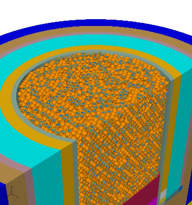
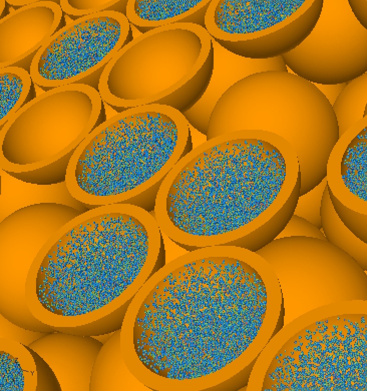
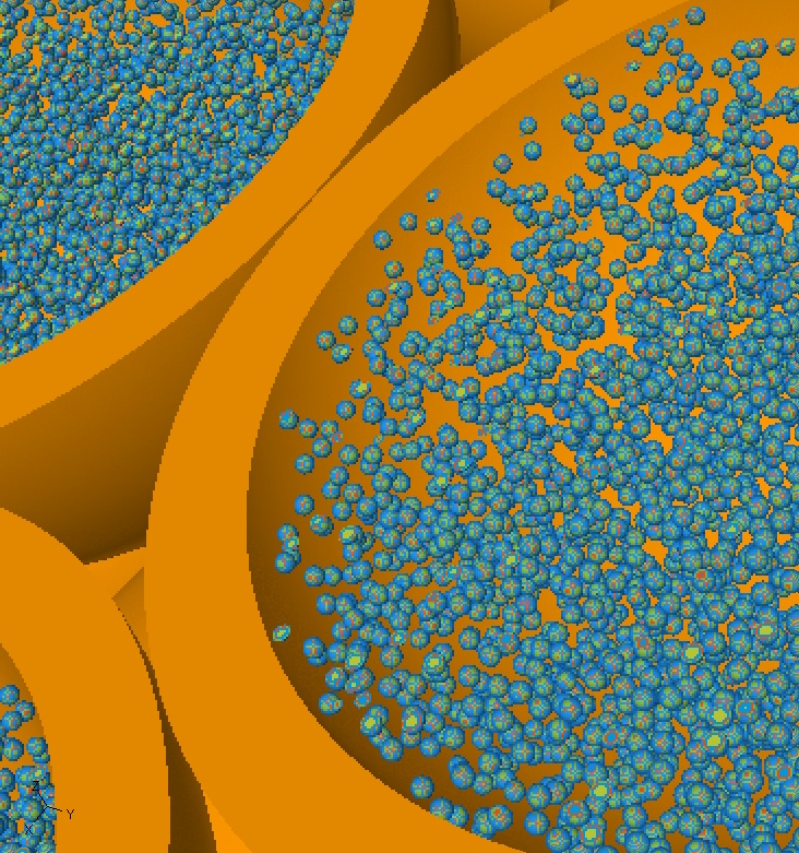
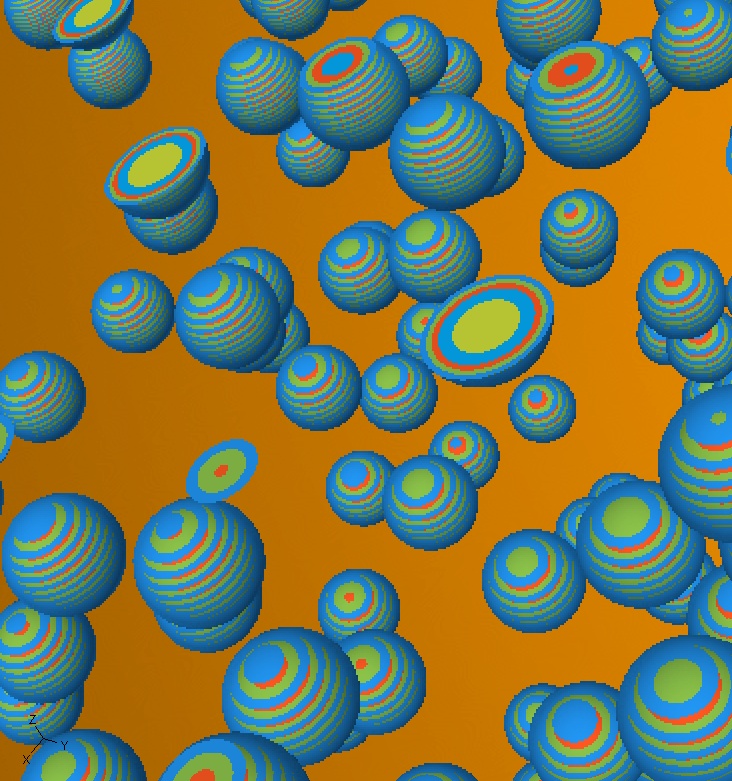
The eigenfunction is called the importance map and offers a quasi-stationary profile of radioactive activity (unless , in which case it is a stationary profile). Indeed, in modern nuclear reactor design and safety regulation, it is usually the case that virtual reactor models such as the one seen in Figure 1 (an example of a uranium pebble bed reactor) are designed such that and the behaviour of within spatial domains on the human scale remains within regulated levels. Existing physics and engineering literature with focus on applications in the nuclear regulation industry, has largely been concerned with different numerical methods for estimating the value of the eigenvalue as well as the eigenfunction and eigenmeasure . Giving a sensible meaning to (3.1) will play an important part in unraveling the analysis of stochastic representations of solutions to the NTE as well. Moreover, in additional forthcoming work [10], we will also see that our asymptotic (3.1), together with the accompanying stochastic analysis developed here, has influence on a number of completely new Monte Carlo methods associated with the NTE that, in turn, bears relevance to the applied NTE literature.
The approximation (3.1) can be seen as a functional version of the Perron-Frobenius Theorem, in particular when noting via (2.8) that we can understand as a semigroup. Many attempts have been made to generalise the notion of the Perron-Frobenius decomposition to semigroups of Markov processes with countable and uncountable state spaces, as well as with killing and mass creation (see for example [14, 33, 34, 35]), using what has come to be known as -theory. The conditions there seem difficult to verify in the current setting.
More recently, [7, 8] have provided an alternative approach to the -theory presented in aforementioned works. In the current context, Theorem 2.1 and Proposition 2.3 of [7] will help us to achieve the global result, given below. To state it we need to introduce the quantity
| (3.2) |
where is taken to be a probability density. As such it necessarily follows that
| (3.3) |
Theorem 3.1.
Suppose that (H1) holds as well as
(H2)∗:
Then, for the semigroup identified by (2.8), there exists a , a positive111To be precise, by a positive eigenfunction, we mean a mapping from . This does not prevent it being valued zero on , as is an open bounded, convex domain. right eigenfunction and a left eigenmeasure which is absolutely continuous with respect to Lebesgue measure on with density , both having associated eigenvalue , and such that (resp. ) is uniformly (resp. a.e. uniformly) bounded away from zero on each compactly embedded subset of . In particular, for all ,
| (3.4) |
Moreover, there exists such that
| (3.5) |
This result differs significantly from what is already in the literature principally through the assumptions on the cross-sections, the strict positivity properties and the uniform boundedness of and uniformity in the mode of convergence. In existing literature (3.5) is usually given in the setting, where is strictly enforced due to the nature of the -semigroup perturbation analysis; cf. [12, 36] and the discussion in [9].
The proof of Theorem 3.1 is a non-trivial application of the recent theory of [7, 8] in that verifying their assumptions (which essentially leads to the full statement of Theorem 3.1) is highly technical, taking account of the dimension of the system and the piecewise linear (and hence irregular) nature of the neutron paths in the underlying NBP.
Once again the assumptions (H3) and (H4) are unnecessary. As we shall shortly see, the result relies on the treatment of the sum of the operators as a single object, re-written as a scattering generator with action
The assumption (H2)∗ is a condition on the intensity of this new generator. In this sense, the need for fission or for control of the pathwise behaviour of number of offspring (other than through their mean) is not needed.
4 Neutron random walk and many-to-one methodology
There is a second stochastic representation of the unique solution to (2.8) which will form the basis of our proof of Theorem 3.1. In order to describe it, we need to introduce the notion of a neutron random walk (NRW).
A NRW on is defined by its scatter rates, , , and scatter probability densities , such that for all . Simply, when issued from with a velocity , the NRW will propagate linearly with that velocity until either it exits the domain , in which case it is killed, or at the random time a scattering occurs, where for When the scattering event occurs in position-velocity configuration , a new velocity is selected with probability . If we denote by , the position-velocity of the resulting continuous-time random walk on with an additional cemetery state for when it leaves the domain , then it is easy to show that is a Markov process. Note, neither nor alone is Markovian. We call the process an -NRW. It is worth remarking that when is given as a single rate function, the density , and hence the rate , is uniquely identified by normalising of the given product form to make it a probability distribution.
To describe the second stochastic representation of (2.8), we define
| (4.1) |
where the lower bound is due to assumption (H1). The following result was established in Lemma 7.1 of [9].
Lemma 4.1 (Many-to-one formula, [9]).
Under the assumptions of Lemma 2.1, we have the second representation
| (4.2) |
where and for the law of the -NRW starting from a single neutron with configuration .
Noting that thanks to (H1), let us introduce for the expectation semigroup of the -neutron random walk with potential , such as is represented by the semigroup (4.2), but now killed at rate . More precisely, for ,
| (4.3) |
where
| (4.4) |
and is an independent exponentially distributed random variable with mean 1.
We will naturally write for the (sub)probability measure associated to , . The family now defines a Markov family of probability measures on the path space of the neutron random walk with cemetery state , which is where the path is sent when hitting the boundary or the clock associated to the killing rate rings. We note for future calculations that we can extend the domain of functions on to accommodate taking a value on by insisting that this value is always 0.
Our strategy for proving Theorem 3.1 thus boils down to understanding the evolution of the semigroup of the NRW . In this sense, we see that the essence of Theorem 3.1 is, roughly speaking, a classical Perron-Frobenius-type problem for the semigroup of a Markov process; namely .
It is also worthy of note that, given the role the -NRW in the proof of Theorem 3.1, we can also interpret the role of the assumptions (H1) and (H2)∗ in terms of this process. The condition (H1) ensures that scattering cannot occur too fast. We can describe the condition (H2)∗ by saying that it offers ‘strong irreducibility’ of the -NRW (where e.g. we could say that (H2) only offers ‘weak irreducibility’).
As alluded to previously, we can also see why the absence of the assumption (H3) is not a problem. In the event that e.g. is identically zero, the original NBP is nothing more than a -NRW, i.e. and . As such the analysis in the proof of Theorem 3.1, which fundamentally concerns a NRW with a ‘strictly irreducible’ state space and killing is still valid. Similarly, the inclusion of (H4) is not necessary as we only need control over the kernel for the purpose of analysing the associated NRW and not the pathwise behaviour of the otherwise associated NBP.
5 The ground state martingale
As an application of the Perron-Frobenius behaviour of the linear semigroups discussed in Theorem 3.1, we complete the summary of the main results of this paper by discussing how the existence of the right eigenfunction plays directly into the existence of a classical (ground state) martingale for the underlying physical process. Analogues of this martingale appear in the setting of all spatial branching processes and is sometimes referred to there as ‘the additive martingale’ (see for example the recent monograph [39] which discusses the analogous setting for branching random walks, or [3] for fragmentation processes).
Under the assumptions of Theorem 3.1 thanks to the semigroup property of (2.4) and the invariance of in Theorem 3.1, it is now easy to see that
| (5.1) |
is a unit mean martingale under where . It is worth noting that this claim is not so easy to make under analogues of Theorem 3.1 found in previous literature (cf. [11, 12, 36]) as the setting of the eigenfunction in an space would make it difficult to make sense of expectations of inner product without saying more about the mean semigroup of .
As a non-negative martingale, the almost sure limit of (5.1) is assured. Our second main result tells us precisely when this martingale limit is non-zero. Before stating the theorem, we require one more assumption on the fission rate and kernel, which is a stricter version of (H3).
(H3)∗: There exists an open ball , compactly embedded in , such that
Theorem 5.1.
For the -NBP satisfying (H1), (H2)∗ and (H4), we have the following cases for the martingale :
-
(i)
If and (H3) holds, then is convergent;
-
(ii)
If and (H3) holds, then almost surely;
-
(iii)
If and (H3)∗ holds, then almost surely.
Although a subtle inclusion, the following theorem also frames Theorem 5.1 in a more tidy way, showing the zero set of the martingale limit agrees with extinction.
Theorem 5.2.
In each of the three cases of Theorem 5.1, we also have that the events and almost surely agree, where is the time of extinction of the NBP. In particular, there is almost sure extinction if and only if .
As we can see from the above theorem, the critical case requires slightly more stringent conditions than the super- or sub-critical cases. However, it we assume the conditions of the critical case across the board, we get the aesthetically more pleasing corollary below.
Corollary 5.3.
For the -NBP satisfying (H1), (H2)∗, (H3)∗ and (H4), the martingale is convergent if and only if and otherwise . Irrespective of , almost surely.
Note that, unlike many spatial branching process (e.g. the classical result of [6]), there is no ‘’ condition thanks to the assumption (H2) and a precise dichotomy on emerges. The result mimics a behavioural trait that has been observed for branching diffusions in compact domains in e.g. [18]. In essence it states that in the competing physical processes of fission, transport, scattering and absorption, it is the lead eigenvalue which dictates growth or decay of mass. In this respect we can also mimic other similar results in the spatial branching process literature (cf. [1, 19, 26]), the proof of which falls out of the proof of Theorem 5.1.
Corollary 5.4.
For the -NBP satisfying the assumptions (H1), (H2)∗, (H3) and (H4), when , the martingale is convergent.
It is particularly interesting to note that in the setting of a critical system, , which is typically what is envisaged for a nuclear reactor, the above results evidences the hypothesis that the fission process eventually dies out (similarly to other examples of critical branching processes).
To verify the aforementioned hypothesis rigorously, one needs an almost sure growth result for the particle system which would take the format
| (5.2) |
-almost surely, for all . This is a much more difficult result than the one stated in Theorem 5.1 and is addressed in a second instalment to this paper; see [20]. The reader should note that (5.2) verifies what has been known in the nuclear industry for a long time. Namely that critical nuclear reactors will not persist in energy generation, but will eventually cease working, corresponding to the case that .
6 Neutron random walk and spine decomposition
As with many spatial branching processes, the most efficient way to analyse martingale convergence is through the pathwise behaviour of the particle system (known as a spine decomposition) when considered under a change of measure induced by the martingale itself. Whilst classical in the branching process literature, it is unknown in the setting of neutron transport. We will devote the remainder of this section to describing the pathwise spine decomposition of the physical process, our final main contribution.
We are interested in the change of measure
| (6.1) |
for the NBP with characteristics (cf. Remark 2.2), where belongs to the space of finite atomic measures .
In the next theorem we will formalise an understanding of this change of measure in terms of another -valued stochastic process
| (6.2) |
which we will now describe through an algorithmic construction.
-
1.
From the initial configuration with an arbitrary enumeration of particles, the -th neutron is selected and marked ‘spine’ with empirical probability
-
2.
The neutrons in the initial configuration that are not marked ‘spine’, each issue independent copies of respectively.
-
3.
For the marked neutron, issue a NRW characterised by the rate function
-
4.
The marked neutron undergoes fission at the accelerated rate , when in physical configuration , at which point, it scatters a random number of particles according to the random measure on given by where
(6.3) -
5.
When fission of the marked neutron occurs in physical configuration , set
and repeat step 1.
The process describes the physical configuration (position and velocity) of all the particles in the system at time , for (i.e. ignoring the marked genealogy). We will also be interested in the configuration of the single genealogical line of descent which has been marked ‘spine’. This process, referred to simply as the spine, will be denoted by . Together, the processes make a Markov pair, whose probabilities we will denote by . Note in particular that
when .
Theorem 6.1.
Under assumptions (H1), (H2) and (H4), the process is Markovian and equal in law to , where .
It is also worth understanding the dynamics of the spine . For convenience, let us denote the family of probabilities of the latter by , in other words, the marginals of .
Next we define the probabilities to describe the law of an -NRW, where
| (6.4) |
for , We are now ready to identify the spine.
Lemma 6.1.
Under assumptions (H1), (H2) and (H4), the process is a NRW equal in law to and, moreover,
| (6.5) |
from which we deduce that is conservative with a stationary distribution on . (Recall that under is the -NRW that appears in the many-to-one Lemma 4.1.)
Now that we have stated all of our main results, it is worth noting that, in places, the analysis echoes very similar issues that have very recently appeared in the analysis of growth-fragmentation equations, see e.g. [5] and [4], and for good reason. Growth-fragmentation equations, although dealing with a particle system in which particles’ mass is positive-valued and for which there is no consideration of classical ‘velocity’, the dynamics of fragmentation shares the phenomenon of non-local branching. This explains the appearance of integral operators. Moreover, a combination of Lévy-type and piecewise linear movement of particles in the growth-fragmentation setting also mirrors the phenomenon of advection and scattering in the NTE and the associated operators.
7 Proof of Theorem 3.1
Our approach to proving Theorem 3.1 will be to extract the existence of the eigentriple , and for the expectation semigroup from the existence of a similar triple of the semigroup defined in (4.3). Indeed, from (4.3), it is clear that when the latter exists, the eigenfunctions of the former are the same and the eigenvalues differ only by the constant .
Throughout this section, we assume the assumptions of Theorem 3.1 are in force.
As alluded to earlier, what lies at the core of our proof is the general result of Theorem 2.1 and Proposition 2.3 of [7] and Theorem 2.1 and the discussion around (1.5) of [8], which, combined in the current context, reads as follows.
Theorem 7.1.
Suppose that there exists a probability measure on such that
-
(A1)
there exist , such that for each ,
-
(A2)
there exists a constant such that for each and for every ,
where k was defined in (4.4). Then, there exists such that, there exists an eigenmeasure on and a positive right eigenfunction of with eigenvalue , such that is a probability measure and , i.e. for all
| (7.1) |
Moreover, there exist such that, for and sufficiently large (which does not depend on ),
| (7.2) |
In particular, setting , as ,
| (7.3) |
We aim to prove that assumptions (A1) and (A2) are satisfied, so that the conclusions of the above theorem hold. Then we prove that is uniformly bounded away from on each compactly embedded subset of and that admits a positive bounded density with respect to the Lebesgue measure on (see Lemma 7.4), which concludes the proof of Theorem 3.1. In order to do so, we start by introducing two alternative assumptions to (A1) and (A2):
There exists an such that
-
(B1)
is non-empty and connected.
-
(B2)
there exist and such that, for all , there exists measurable such that and for all , for every and for all .
It is easy to verify that (B1) and (B2) are implied when we assume that is a non-empty convex domain, as we have done in the introduction. They are also satisfied if, for example, the boundary of is a smooth, connected, compact manifold and is sufficiently small. Geometrically, (B2) means that each of the sets
| (7.4) |
is included in and has Lebesgue measure at least . Roughly speaking, for each which is within of the boundary , is the set of points from which one can issue a neutron with a velocity chosen from such that (ignoring scattering and fission) we can ensure that it passes through during the time interval .
Our proof of Theorem 3.1 thus consists of proving that assumptions (B1) and (B2) imply assumptions (A1) and (A2). Our method is motivated by [7, Section 4.2], however, we note that our approach accommodates for the more general setting we have here (e.g. is bounded and ) at the cost of greater technicalities.
We begin by considering several technical lemmas. The first is a straightforward consequence of being a bounded subset of .
Lemma 7.1.
Let be the ball in centred at with radius .
-
(i)
There exists an integer and such that and for each .
-
(ii)
For all , there exists and distinct in such that , and for all , .
Heuristically, the above lemma ensures that there is a universal covering of by the balls , such that between any two points in , there is a sequence of overlapping balls that one may pass through in order to get from to .
The next lemma provides a minorization of the law of under . The result is similar to [7, Lemma 4.5], however, we provide a less geometrical proof by considering a change of variables from Cartesian to polar coordinates. In the statement of the lemma, we use for the distance of from the boundary .
Define and . We will also similarly write and with obvious meanings. We note that due to the assumption (H1) we have and and hence, combining this with (H2)∗ it follows that,
and a similar calculation shows that .
Lemma 7.2.
For all , and such that , the law of under , defined in (4.3), satisfies
| (7.5) |
where is a positive constant.
Proof.
Fix . Let denote the jump time of under and let be uniformly distributed on . Assuming that , we first give a minorization of the density of , with initial configuration , on the event . Note that, on this event, we have
where is the velocity of the process after the first jump. Then
| (7.6) |
where we have used the bounds on and . We now make the change of variables and so that (7.6) becomes
| (7.7) | ||||
where
| (7.8) |
represents the spatial variable in polar coordinates,
| (7.9) |
represents in polar coordinates,
| (7.10) |
is the determinant of the Jacobian matrix for the change of variables from Cartesian to polar coordinates, and is an unimportant normalising constant.
For fixed , , and , we first consider the part of (7.7) given by
| (7.11) |
The Jacobian of , as a function of , is given by
whose determinant, satisfies
We thus have the following lower bound for (7.11)
| (7.12) | |||
Making another change of variables and using the fact that, regardless of the values of , and , maps surjectively onto a set that contains , where is the ball in of radius centred at the origin, (7.12), and hence (7.11), is bounded below by
| (7.13) |
Substituting this equation back into (7.7) and changing back to Cartesian coordinates, we have
| (7.14) |
where .
Now suppose we fix an initial configuration , with . By considering the event and noting that the scattering kernel is bounded below by , we may apply the Markov property together with (7.14) to the process at time before choosing the new velocity. Using the bounds on and as before, and recalling that is uniformly distributed, we have
| (7.15) |
where we have used the substitution to obtain the final line and is another constant in . Now note that for we have . Combining this with (7.15) and using Fubini, we have
| (7.16) |
We finally compute the integral with respect to . In order to do so, we first note that since , the integrand in (7.16) is bounded below by
Absorbing into the constant , applying Fubini and computing the integral yields
| (7.17) |
as required. ∎
We now turn to the proof of (A1) under the assumptions of (B1) and (B2).
Proof of (A1).
In this proof, we will follow a similar strategy to the one presented in [7, Section 4.2]. We therefore start by proving (A1) for initial configurations in .
To this end, fix . From Lemma 7.1, there exists an such that . Then, for each , Lemma 7.2 yields
| (7.18) |
Now, if is such that , the triangle inequality implies that , with the latter inclusion following from the fact that .
Hence, for and , the density on the right-hand side of (7.18) is bounded below by a constant , which is independent of and . Hence,
| (7.19) |
Now let . By writing , for some and . We will demonstrate that a repeated application of (7.19) will lead to the inequality
| (7.20) |
for , where is another unimportant constant which depends only on and is defined in the following analysis.
To this end, we start by noting that, since and , there exists such that and . Applying (7.19) at time (recall that we have identified for some ) we obtain,
| (7.21) |
We now turn our attention to , for and . Thanks to Lemma 7.1, for all , there exist such that for every . Note, here we see the importance of choosing , to ensure the validity of the previous statement.
Applying (7.19) and following the same steps that lead to (11.3), we obtain
| (7.22) |
Iterating this step a further times, we obtain
| (7.23) |
where . Using this inequality to bound the right-hand side of (11.3) yields
| (7.24) |
We now apply (7.19) a final time at time to obtain
| (7.25) |
Since this inequality holds for every , it also follows that
where the final line follows from Lemma 7.1 since . This is the lower bound claimed in (7.20).
Finally, noting that for any two events , , we have that for initial conditions , any and equal to Lebesgue measure on , there exists a constant such that
as required by (A1).
We now prove (A1) for initial conditions in . Once again, we recall that assumptions (B1) and (B2) are in force.
Choose , and define the (deterministic) time
which is the time it would take a neutron released at with velocity to hit the boundary of if no scatter or fission took place. Note in particular that is not a random time but entirely deterministic. We first consider the case
| (7.26) |
Combining this with (7.20) and the Markov property, for all
| (7.27) |
where is such that for some .
On the other hand, suppose . Then, recalling the assumptions (B1) and (B2) it follows that . Heuristically speaking, this is because if the first jump occurs before time , then the process hasn’t hit the boundary and there are still (at least) units of time left until . By then choosing the new velocity, , from , thanks to the assumption (B1) and the remarks around (7.4), this implies that the process will remain in for units of time, at some point in time after which, it will move into , providing the process doesn’t jump again before entering . Combining this with the usual bounds on , and recalling from (B2) that for all and , we have
| (7.28) |
Along with (7.20), this implies that, for all , and such that
| (7.29) |
Now, since we are considering the case and , it follows that . Then,
| (7.30) |
with the bound on the right-hand side above being itself bounded below by a constant that does not depend on . Substituting this back into (7.29), this proves (A1) with taken as Lebesgue measure on as before, can be sufficiently taken as and we may start with any initial configurations in . ∎
In order to prove (A2) we require the following lemma, the proof of which will be given after that of (A2).
Lemma 7.3.
For all and , recalling that denotes the jump time of the process , we have
| (7.31) |
for some constant , and
| (7.32) |
for another constant , where , from the proof of (A1), is Lebesgue measure on .
Proof of (A2).
Again, we follow the proof given by the authors in [7]. Let and note that on the event , we have almost surely. This inequality along with the strong Markov property imply that,
| (7.33) |
Since is uniformly bounded above, conditional on , the density of is bounded above by multiplied by Lebesgue measure on . Combining this with (7.31) and (7.33), we obtain
| (7.34) |
for some Similarly, for , equation (7.32), the fact that the inclusion , the strong Markov property and the fact that is uniformly bounded below entail that,
for some , where is Lebesgue measure on . Putting (7.33) and (7.34) together, for all , we have
| (7.35) |
Now, recalling and from the proof of (A1), it follows from (A1) that
| (7.36) |
The event occurs if the particle has either been killed on the boundary of or if it has been absorbed by fissile material, which occurs at rate . Since and are fixed, and by assumption, for some constant . Thus, keeping , using (7.36)
| (7.37) |
where .
Proof of Lemma 7.3.
Let us first prove (7.31). Again, following the proof given in [7], we couple the neutron transport random walk in with one on the whole of . Denote by the neutron random walk in , coupled with such that and for all and , for , . Denote by the jump times of . Then for each such that , we have . Due to the inequality
| (7.40) |
we will consider the distribution of for . We first look at the case when . For and non-negative, bounded, measurable functions ,
| (7.41) |
For fixed, we consider the integrals over and in (7.41). Making the change of variables , we have
| (7.42) |
where was defined in (7.9). Now making the substitution in (7.42),
| (7.43) |
where . Making a final change of variables , we have
| (7.44) |
Substituting this back into (7.41) yields
| (7.45) |
where . Iterating this process over the next five jumps of the process gives
where , . Now, for each so that, in particular, . Hence, repeatedly applying Young’s inequality implies that the six-fold convolution . (The reader will note that this is the fundamental reason we have focused our calculations around the 7th jump time , rather than it being an arbitrary choice.) Making the substitution ,
| (7.47) |
Finally, setting yields
| (7.48) |
where , which completes the proof of (7.31).
We now prove (7.32). For , let denote the line segment between and . For all , recalling the definition of from the proof of (A1) and using the usual bounds on ,
| (7.49) |
where and . Following a similar method to those employed in the proof of Lemma 7.2 and (7.31) and changing first to polar coordinates via , followed by the substitution , and finally changing back to Cartesian coordinates via , the right-hand side of (7.49) is bounded below by
| (7.50) |
where is a constant. Making a final substitution of , yields
| (7.51) |
For all , (B1) and the discussion thereafter now imply that
| (7.52) |
where and are defined in (B2), and is defined in (7.4). On the other hand, for all ,
| (7.53) |
Since the map is continuous and positive on the compact set , the latter equation is uniformly bounded below by a strictly positive constant. It then follows that for every , the integral is bounded below by a positive constant. Using this to bound the right-hand side of (7.51) yields the result. ∎
We thus have proved that the conclusions of Theorem 7.1 are valid under our assumptions. In order to conclude that Theorem 3.1 holds true, it remains to prove that is uniformly bounded away from 0 on each compactly embedded subset of and the existence of a positive bounded density for the left eigenmeasure .
Lemma 7.4.
The right eigenfunction is uniformly bounded away from on each compactly embedded subset of and the probability measure admits a positive density with respect to the Lebesgue measure on , which corresponds to the quantity and which is uniformly bounded from above and a.e. uniformly bounded from below on each compactly embedded subset of .
Proof.
For all , we deduce from the eigenfunction property of (cf. Theorem 7.1) and from (7.20) that there exist a time and a constant such that
for all . It follows that is uniformly bounded away from 0 on each compactly embedded domain of .
Using the same notations as in the proof of Lemma 7.3, we consider the neutron transport random walk in , coupled with such that and for all . We also denote by the jump times of . Let be a random time independent of with uniform law on , where are fixed and . We first prove that the law of after the jump admits a uniformly bounded density with respect to the Lebesgue measure. We conclude by using the coupling with and the quasi-stationary property of in (7.1).
For all and for any positive, bounded and measurable function vanishing outside of , we have
Henceforth
Taking the expectation with respect to , we obtain
Using the change of variable yields
The same approach as in Lemma 7.3 shows that there exists a constant (which does not depend on nor on ) such that, for all measurable function ,
Hence,
where we used the change of variable and the fact that vanishes outside . Summing over , we deduce that there exists a constant (which only depends on and ) such that
Similarly as in the proof of (A2), we chose , so that, on the event , we have almost surely. Hence, we obtain that, for any ,
Integrating with respect to and using the quasi-stationary property (7.1) and Fubini’s Theorem (recall that and the process are independent), we obtain
| (7.54) |
Since was chosen arbitrarily, this proves that admits a uniformly bounded density (from above) with respect to the Lebesgue measure on .
Finally, using the quasi-stationarity of (7.1) and integrating inequality (7.19) with respect to implies that (here the time and the constants depend on as in inequality (7.20)), for all bounded measurable functions on ,
This implies that is a.e. lower bounded by on . Since this inequality can be proved for any small enough, one deduces that, on any subset with and hence on any compactly embedded subset of , is a.e. uniformly bounded away from zero. ∎
8 Proof of Theorem 6.1
There are three main steps to the proof. The first is to characterise the law of transitions of the Markov process , defined in the change of measure (6.1); note that the latter ensures the Markov property is preserved. The second step is to show that they agree with those of . The third step is to show that is Markovian. Together these three imply the statement of the theorem.
Step 1. Next we look at the multiplicative semigroup which characterises uniquely the transitions of (cf. [22, 23, 24])
| (8.1) |
for and which is uniformly bounded by unity. Note, we keep to the convention that an empty product is understood as 1, however we also define the empty inner product as zero (corresponding to all functions scoring zero when particles arrive at the cemetery state ). As such, if we are to extend the domain of test functions in the product to include the cemetery state , we need to insist on the default value ; see [22, 23, 24].
We start in the usual way by splitting the expectation in the second equality of (8.1) according to whether a scattering or fission event occurs. (The reader may wish to recall the role of the quantities , , , and in (1.1)). We get
| (8.2) |
where, for , , and are independent copies of the pair and under . Note that the first term on the right-hand side of (8.2) contains includes to account for the fact that . Before developing the right-hand side above any further, we need to make two additional observations and to introduce some more notation.
The first observation is that, since is a martingale, by sampling at the time of the first scattering event, fission event or when it leaves the domain , whichever happens first, thanks to Doob’s Optional Sampling Theorem, its mean must remain equal to 1 and we get the functional equation
| (8.3) |
for , . Now appealing to Lemma 1.2, Chapter 4 in [16], to treat the last two terms of (8.3) as potentials, with a little bit of algebra we can otherwise write the above as
for , where I is the identity operator, which is to say, for ,
| (8.4) |
Our second observation pertains to the manipulation of the expectation on the right-hand side of (8.2). Define for , and ,
| (8.5) |
We have that for all ,
| (8.6) |
where in the penultimate equality we have taken expectations conditional on the fission event and
| (8.7) |
for , which are uniformly bounded by unity, and for , , where we recall that was defined in (6.3). Note in particular that
| (8.8) |
We will also make use of the notation
| (8.9) |
for , and , which is uniformly bounded by unity. Recall that the empty product in the definition (8.10) is defined as unity.
In a similar manner to (8.2) we can break the expectation over the event of scattering or fission in (8.10), which defines of , to see that the operator appears in the decomposition
| (8.10) |
for , which is uniformly bounded by unity. Here, we have adjusted the definition of the semigroup U to
| (8.11) |
Now returning to (8.2) with the above observations and definitions in hand, whilst again appealing to Lemma 1.2, Chapter 4 in [16], we have
| (8.12) | ||||
| (8.13) |
where where
on and otherwise equal to zero,
Step 2. Define
| (8.14) |
for , where are the physical configurations of the particles alive in the system at time in .
By conditioning on the first time a scattering of fission event occurs, it is a straightforward exercise to show that it also solves (8.13). For the sake of brevity, we leave this as an exercise to the reader as the arguments are similar to those mentioned previously. In order to show that (8.13) has a unique solution, we consider and . Since and both satisfy (8.12), applying [16, Lemma 1.2, Chapter 4] along with (8.4), it is straightforward to show that and both satisfy
| (8.15) |
where
Due to the assumptions (H1) and (H4), an application of Grönwall’s inequality implies uniqueness of (8.15), which in turn implies uniqueness of (8.13). We leave this as an exercise to the reader as it is a relatively standard computation and very similar to the calculations given in [9].
Step 3. We start by noting that the joint process is, by construction, Markovian under , we thus need to show that the marginalisation of the coupled system to just retains the Markov property. We do this by showing that for , and ,
| (8.16) |
This says that knowing only allows one to construct the law of through an empirical distribution using . Hence, for which is bounded by unity and ,
where we have written , and thus the Markov property of follows.
We are thus left with proving (8.16) to complete this step. To do so we note that it suffices to show that for bounded by unity, and ,
| (8.17) |
On the left-hand side of (8.17), we have
where , , are the times of fission along the spine at which point particles are issued at , . On the right-hand side of of (8.17), we may appeal to Step 1 and Step 2 to deduce that
The proof of this final step is thus complete as soon as we can show that
| (8.18) |
To this end, we note that splitting the expectation on the right-hand of (8.18) side at either a scattering or fission event results in a calculation that is almost identical to the one above that concludes with (8.13). More precisely, the expectation on the right-hand side solves (8.13) albeit the role of is replaced by . Similarly splitting the expectation on the left-hand side of (8.18) also results in a solution to (8.13) (with the aforementioned adjustment). The uniqueness of (8.13), with replaced by U, follows from the same arguments and hence the equality in (8.18) now follows, as required.
9 Proof of Lemma 6.1
The fact that the spine is Markovian is immediate from its definition of . Indeed, once given its initial configuration, it evolves as the NRW associated to the rate . Moreover, when in configuration , at rate , it experiences an additionally scattering with new velocity , with distribution
for , where we have used (8.8). The total scatter rate is thus
| (9.1) | |||
as required.
For the second statement, write
| (9.2) |
By conditioning the expectation on the right-hand side on the first scattering event we have, for , and ,
| (9.3) |
Now appealing to (8.4), then using the standard trick of replacing the role of an additive potential by the role of a multiplicative potential in such semigroup evolutions, see e.g. Lemma 1.2, Chapter 4 in [16], and noting (9.2) we get
| (9.4) |
where
| (9.5) |
for . Referring to (2.6), (2.7) and (4.1), we note that
Hence (9.4) reduces to the somewhat simpler recurrence equation
where we recall that was defined in (9.5). This is nothing more than the mild equation for the semigroup evolution , , which has a unique bounded solution from the usual Grönwall arguments. Note that when , we see the solution is 1. This, together with the Markov property implies that the right-hand side of (6.5) is a martingale. Moreover, it follows that the martingale change of measure in (6.5) describes law of the -NRW.
The fact that for all , implies that is conservative. Moreover,
where ; cf. (9.2). Hence for all . In other words, is the density of the stationary distribution of under .
10 Proof of Theorem 5.1
The proof we offer here is a variant of a standard one, which has been used to analyse the convergence of many analogous martingales in the setting of different spatial branching processes. We mention [31], [39], [3] and [17] to name but a few of the contexts with similar results.
In the case that and , we need (H3) to ensure that the NBP can undergo fission. In the setting we need the stricter condition (H3)∗ for technical reasons in the proof to ensure a minimal rate of reproduction.
A standard measure theoretic result (cf. p. 242 of [15]) tells us that the martingale change of measure in (6.1) is uniformly integrable if and only if
In the case that , almost surely, we have .
(i) Let us first deal with the case that . To this end, let us define the sigma algebra , where , , are the times at which the spine undergoes fission and , , are point processes on that describe the velocities of fission offspring (i.e. whose law is given by the family (2.2) under the change of measure (6.3)). For convenience we will write .
Appealing to the pathwise spine decomposition in Theorem 6.1, we can write
| (10.1) |
where, for a given , the process is an independent copy of , under (and consequently has unit mean, which is also used above). Our objective is to prove that the sum on the right-hand side of (10.1) is -almost surely finite. In that case, it will follow with the help of Fatou’s Lemma that
| (10.2) |
Recalling that is a non-negative -martingale, it holds that is a non-negative -supermartingale and thus its limit exists. The conditional expectation in (10.2) ensures that (and hence from the immediately preceding remarks ) is -almost surely finite.
We must thus show that the upper bound on the right-hand side of (10.1) is -almost surely finite. To do so, we again recall the description of the pathwise spine decomposition in Theorem 6.1 and note that fission along the spine occurs at the accelerated rate . Hence (recalling the generic point process defined in (2.2))
| (10.3) |
where we have used (H4) in the first inequality, features of the spine decomposition for the first equality, (8.8) and (H1) in the second inequality, the change of measure (6.5) in the third inequality and the semigroup (4.2) for the final line. Finally, note that since is uniformly bounded above, the contribution from the spine term in (10.1) is zero in the limit . Now using Theorem 3.1, it follows that
as required.
(ii) Next, for the case , it is easy to see that, on the event ,
which ensures that for all and hence .
(iii) Finally, for the case , our aim is to show that, for each ,
We do this by constructing a random sequence of times such that almost surely with respect to .
Lemma 6.1 tells us that is the density of the stationary distribution of under . Moreover, thanks to Theorem 3.1, the density is a.e. uniformly bounded away from on each . It follows that for all and that the spine visits infinitely often under .
Fix . We want to show that there is an such that
| (10.4) |
where (note that is twice the time it would take a neutron to cross the equivalent of the diameter of , when moving at minimal speed). To this end, fix and choose sufficiently small such that both and (introduced in the assumption (H3)∗) is in . Then, define
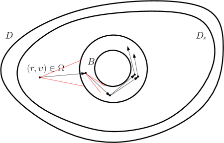
Write for the smallest natural number such that . Recalling from Theorem 3.1 that , and taking account of the positivity properties of , we can lower bound the probability that, from any , the spine can enter . Moreover, on this event, due to (H3)∗, we can also lower bound the probability that the spine immigrates particles on (evenly spaced in time) separate occasions, all of which are still inside of by time . The strategy for doing so is to head into from the given point of issue in by travelling in a straight line within a small cone of possible velocities (which would be guaranteed to happen within units of time), and then for neutrons to cycle around the perimeter of in an annulus by scattering within a narrow cone of velocities each time; see Fig 2. As such we can provide the lower bound desired in (10.4). The technical details are tedious and left to the reader.
With (10.4) in hand, we can construct the sequence by defining and subsequently, for ,
Note that since visits infinitely often under we have that , -almost surely for , and , -almost surely. By applying the strong Markov property at the sequence of times , it now follows from (10.4) that, in the spirit of a sequence of independent Bernoulli trials, almost surely with respect to , where . Since the integer can be chosen arbitrarily large, we also have that almost surely with respect to .
As is uniformly bounded below away form 0 on (see Theorem 3.1), it follows that
for some constant . The analysis above, thus shows that , as required, for each , .
11 Proof of Theorem 5.2
We need to show that in all three cases, the event agrees almost surely with . To this end, first note that and hence
| (11.1) |
for all , . It thus suffices to show that (11.1) is in fact an equality.
We will give two preparatory technical lemmas before coming to the main part of the proof of Theorem 5.2.
Lemma 11.1.
For all and , we have -almost surely that
Proof.
On the event , it is immediate that, for all and ,
| (11.2) |
-almost surely. Let be any increasing sequence of stopping times. Using the strong Markov property and (11.2), we have that, for all ,
Using this inequality and Fatou’s Lemma, we deduce that
It follows that, for all , we have . This implies that, on , Since this is true for any sequence of increasing stopping times, we deduce that, on , Together with (11.2), this gives us
-almost surely, as required. ∎
Lemma 11.2.
For all and , on , we have -almost surely that
| (11.3) |
Proof.
Recall that is the time of extinction of the NBP. For any , and , we have
Using (3.5), we deduce that there exists a such that, for all , ,
It is straightforward to show that . Hence, there exists a constant such that, uniformly for all and ,
Using the branching property, we deduce that, for all ,
Now, using the Lemma 11.1 we have, taking the limit in , we obtain
| (11.4) |
where we have used the notation from (2.1). Since , taking logarithms in (11.4) and using , we deduce that, on , again taking limits on ,
and hence the statement of the lemma follows. ∎
Let us now return to the proof of Theorem 5.2. First we consider the setting that . Noting that, up to a normalising constant , as is almost surely convergent, the conclusion of Lemma 11.2 forces us to deduce that almost surely in order to avoid a contradiction. Hence, from (11.1), we have that and both occur with probability one (irrespective of the starting configuration of ).
Next we consider the setting that . Due to our assumptions and the boundedness of , we have uniformly, for all , and all times such that there is a discontinuity in , is uniformly bounded by some constant , almost surely. Defining the stopping time , using the fact that is a non-negative, , and hence uniformly integrable martingale, and using Doob’s Optional Stopping Theorem, we deduce that, for all , ,
It follows that, for all and , . Hence that there exists such that
Now, using the branching property, we obtain for all ,
Due to the conclusion of Lemma 11.2 we have, on ,
With the upper bound of any probability being unity, we can thus write
Markov’s property now entails, for , ,
so that, by the Reverse Fatou’s Lemma,
Together with (11.1), this completes the proof of the theorem.
12 Proof of Corollary 5.4
Doob’s martingale inequality ensures that, for
Showing that the right-hand side above is finite is sufficient to obtain convergence. Note, however, that , , and hence, from (10.2), the desired upper bound is proved.
Acknowledgements
This research was born out of a surprising connection that was made at the problem formulation “Integrative Think Tank” as part of the EPSRC Centre for Doctoral Training SAMBa in the summer of 2015. AEK and EH are indebted to Professor Paul Smith and Dr. Geoff Dobson from the ANSWERS modelling group at Wood for the extensive discussions at their offices in Dorchester as well as for giving permission to use these images in Figure 1, which were constructed with Wood nuclear software ANSWERS. We would also like to thank Alex Cox, Simon Harris and Minmin Wang for helpful discussions, as well as Jean Bertoin and Alex Watson for several interesting discussions on growth-fragmentation equations. Finally, we are extremely grateful to the assistance of an AE and an anonymous referee, which have helped us shape the presentation significantly.
References
- [1] G. Alsmeyer and A. Iksanov. A log-type moment result for perpetuities and its application to martingales in supercritical branching random walks. Electron. J. Probab., 14:no. 10, 289–312, 2009.
- [2] G. I. Bell. On the stochastic theory of neutron transport. Nuc. Sci. & Eng., 21:390–401, 1965.
- [3] J. Bertoin. Random fragmentation and coagulation processes, volume 102 of Cambridge Studies in Advanced Mathematics. Cambridge University Press, Cambridge, 2006.
- [4] J. Bertoin. On a Feynman-Kac approach to growth-fragmentation semigroups and their asymptotic behaviors. J. Funct. Anal., 2019. In Press.
- [5] J. Bertoin and A. R. Watson. A probabilistic approach to spectral analysis of growth-fragmentation equations. J. Funct. Anal., 274(8):2163–2204, 2018.
- [6] J. D. Biggins. Martingale convergence in the branching random walk. J. Appl. Probab., 14(1):25–37, 1977.
- [7] N. Champagnat and D. Villemonais. Exponential convergence to quasi-stationary distribution and -process. Probab. Theory Related Fields, 164(1-2):243–283, 2016.
- [8] N. Champagnat and D. Villemonais. Uniform convergence to the -process. Electron. Commun. Probab., 22:7 pp., 2017.
- [9] A. M. G. Cox, S. C. Harris, E. L. Horton, and Andreas E. Kyprianou. Multi-species neutron transport equation. J. Stat. Phys., 176(2):425–455, 2019.
- [10] A. M. G. Cox, S.C. Harris, E. Horton, A.E. Kyprianou, and M. Wang. Monte carlo methods for the neutron transport equation. Working document, 2018.
- [11] R. Dautray, M. Cessenat, G. Ledanois, P.-L. Lions, E. Pardoux, and R. Sentis. Méthodes probabilistes pour les équations de la physique. Collection du Commissariat a l’énergie atomique. Eyrolles, Paris, 1989.
- [12] R. Dautray and J.-L. Lions. Mathematical analysis and numerical methods for science and technology. Vol. 6. Springer-Verlag, Berlin, 1993. Evolution problems. II, With the collaboration of Claude Bardos, Michel Cessenat, Alain Kavenoky, Patrick Lascaux, Bertrand Mercier, Olivier Pironneau, Bruno Scheurer and Rémi Sentis, Translated from the French by Alan Craig.
- [13] B. Davison and J. B. Sykes. Neutron transport theory. Oxford, at the Clarendon Press, 1957.
- [14] D. Down, S. P. Meyn, and R. L. Tweedie. Exponential and uniform ergodicity of Markov processes. Ann. Probab., 23(4):1671–1691, 1995.
- [15] R. Durrett. Probability: Theory and Examples. Duxbury, Belmont, CA, 1996.
- [16] E. B. Dynkin. Diffusions, superdiffusions and partial differential equations, volume 50 of American Mathematical Society Colloquium Publications. American Mathematical Society, Providence, RI, 2002.
- [17] János Engländer and Andreas E. Kyprianou. Local extinction versus local exponential growth for spatial branching processes. Ann. Probab., 32(1A):78–99, 2004.
- [18] S. N. Ethier and T. G. Kurtz. Markov processes. Wiley Series in Probability and Mathematical Statistics: Probability and Mathematical Statistics. John Wiley & Sons, Inc., New York, 1986. Characterization and convergence.
- [19] R. Hardy and S. C. Harris. A spine approach to branching diffusions with applications to -convergence of martingales. In Séminaire de Probabilités XLII, volume 1979 of Lecture Notes in Math., pages 281–330. Springer, Berlin, 2009.
- [20] S.C. Harris, E. Horton, and A.E. Kyprianou. Stochastic analysis of the neutron transport equation II: Almost sure growth. Preprint, 2018.
- [21] T. E. Harris. The theory of branching processes. Dover Phoenix Editions. Dover Publications, Inc., Mineola, NY, 2002. Corrected reprint of the 1963 original [Springer, Berlin; MR0163361 (29 #664)].
- [22] N. Ikeda, M. Nagasawa, and S. Watanabe. Branching Markov processes. I. J. Math. Kyoto Univ., 8:233–278, 1968.
- [23] N. Ikeda, M. Nagasawa, and S. Watanabe. Branching Markov processes. II. J. Math. Kyoto Univ., 8:365–410, 1968.
- [24] N. Ikeda, M. Nagasawa, and S. Watanabe. Branching Markov processes. III. J. Math. Kyoto Univ., 9:95–160, 1969.
- [25] K. Jörgens. An asymptotic expansion in the theory of neutron transport. Comm. Pure Appl. Math., 11:219–242, 1958.
- [26] A. E. Kyprianou and A. Murillo-Salas. Super-Brownian motion: -convergence of martingales through the pathwise spine decomposition. In Advances in superprocesses and nonlinear PDEs, volume 38 of Springer Proc. Math. Stat., pages 113–121. Springer, New York, 2013.
- [27] B. Lapeyre, É. Pardoux, and R. Sentis. Introduction to Monte-Carlo methods for transport and diffusion equations, volume 6 of Oxford Texts in Applied and Engineering Mathematics. Oxford University Press, Oxford, 2003. Translated from the 1998 French original by Alan Craig and Fionn Craig.
- [28] J. Lehner. The spectrum of the neutron transport operator for the infinite slab. J. Math. Mech., 11:173–181, 1962.
- [29] J. Lehner and G. M. Wing. On the spectrum of an unsymmetric operator arising in the transport theory of neutrons. Comm. Pure Appl. Math., 8:217–234, 1955.
- [30] J. Lehner and G. M. Wing. Solution of the linearized Boltzmann transport equation for the slab geometry. Duke Math. J., 23:125–142, 1956.
- [31] R. Lyons. A simple path to Biggins’ martingale convergence for branching random walk. In Classical and modern branching processes (Minneapolis, MN, 1994), volume 84 of IMA Vol. Math. Appl., pages 245–249. Springer, New York, 1997.
- [32] S. Maire and D. Talay. On a Monte Carlo method for neutron transport criticality computations. IMA J. Numer. Anal., 26(4):657–685, 2006.
- [33] S. P. Meyn and R. L. Tweedie. Stability of Markovian processes. I. Criteria for discrete-time chains. Adv. in Appl. Probab., 24(3):542–574, 1992.
- [34] S. P. Meyn and R. L. Tweedie. Stability of Markovian processes. II. Continuous-time processes and sampled chains. Adv. in Appl. Probab., 25(3):487–517, 1993.
- [35] S. P. Meyn and R. L. Tweedie. Stability of Markovian processes. III. Foster-Lyapunov criteria for continuous-time processes. Adv. in Appl. Probab., 25(3):518–548, 1993.
- [36] M. Mokhtar-Kharroubi. Mathematical topics in neutron transport theory, volume 46 of Series on Advances in Mathematics for Applied Sciences. World Scientific Publishing Co., Inc., River Edge, NJ, 1997. New aspects, With a chapter by M. Choulli and P. Stefanov.
- [37] I. Pázsit and L. Pál. Neutron Fluctuations: A Treatise on the Physics of Branching Processes. Elsevier, 2008.
- [38] A. Pazy and P. H. Rabinowitz. A nonlinear integral equation with applications to neutron transport theory. Arch. Rational Mech. Anal., 32:226–246, 1969.
- [39] Z. Shi. Branching random walks, volume 2151 of Lecture Notes in Mathematics, Lecture notes from the 42nd Probability Summer School held in Saint Flour, 2012, École d’Été de Probabilités de Saint-Flour. Springer, 2015.
| Glossary of some commonly used notation | ||
| (Th. = Th., a. = above, b. = below) | ||
| Notation | Description | Introduced |
| Solution to mild NTE/NBP expectation semigroup | (2.4), (2.8) | |
| and | Physical and velocity domain | §1 |
| , and | Scatter, fission and total cross-sections | b. (1.1) |
| and | Scatter and fission kernels | b. (1.1) |
| S and F | Scatter and fission operators | (2.6), (2.7) |
| Offspring law of when parent at | (2.3) | |
| Position and number of offspring positions of a family in | a. (2.2) | |
| NBP when issued from | §2.2 | |
| Linear advection semigroup | b. (2.5), (2.8) | |
| Branching generator of | (8.9) | |
| Non-linear semigroup of | (8.10) | |
| Non-linear advection semigroup | (8.10), (8.11) | |
| Maximum number of neutrons in a fission event | b. (2.3), (H4) | |
| , and | Leading eigenvalue, right- and left-eigenfunctions | Th. 3.1 |
| Additive martingale | (5.1) | |
| Extinction time | Th. 5.1 | |
| Many-to-one NRW | Lemma 4.1 | |
| and | Scatter rate and kernel for many-to-one NRW | (3.2), (3.3) |
| First exit time of spatial component of -NRW from | Lemma 4.1 | |
| Killed -NRW | (4.3) | |
| Semigroup of killed -NRW | (4.3) | |
| Many-to-one potential | (4.1), (4.2) | |
| k | Killing time of -NRW | (4.4) |
| Ordered jump times of killed -NRW | b. (7.5) | |
| NBP after change of measure with when issued from | (6.1) | |
| Branching generator of | (8.7), (8.13) | |
| Non-linear semigroup of | (8.1) | |
| Linear semigroup of | (9.2) | |
| Dressed spine when issued from configuration | (6.2) | |
| Non-linear semigroup of | (8.14) | |
| Marginal of giving law of spine NRW | Th. 6.1, (6.5) | |
| and | Scatter rate and kernel of auxiliary NRW | (6.4) |
| Scattering of velocities along the spine | (6.3) | |
| Law of -NRW that agrees with | a. (6.4) |