Measurement of the top quark mass in the $t\bar{t}\to$ lepton+jets channel from $\sqrt{s}=8$ TeV ATLAS data and combination with previous results TOPQ-2017-03 CERN-EP-2018-238 Eur. Phys. J. C 79 (2019) 290 10.1140/epjc/s10052-019-6757-9 The top quark mass is measured using a template method in the $t\bar{t}\to\mathrm{lepton+jets}$ channel (lepton is $e$ or $\mu$) using ATLAS data recorded in 2012 at the LHC. The data were taken at a proton–proton centre-of-mass energy of ${\sqrt{s}}=8$ TeV and correspond to an integrated luminosity of $20.2$ fb^-1. The $t\bar{t}\to\mathrm{lepton+jets}$ channel is characterized by the presence of a charged lepton, a neutrino and four jets, two of which originate from bottom quarks ($b$). Exploiting a three-dimensional template technique, the top quark mass is determined together with a global jet energy scale factor and a relative $b$-to-light-jet energy scale factor. The mass of the top quark is measured to be $m_{\mathrm{top}}=172.08\,\pm\,0.39\,\mathrm{(stat)}\,\pm\,0.82\,\mathrm{(syst)}$ GeV. A combination with previous ATLAS $m_{\mathrm{top}}$ measurements gives $m_{\mathrm{top}}=172.69\,\pm\,0.25\,\mathrm{(stat)}\,\pm\,0.41\,\mathrm{(syst)}$ GeV.

1 Introduction

The mass of the top quark $m_{\mathrm{top}}$ is an important parameter of the Standard Model (SM). Precise measurements of $m_{\mathrm{top}}$ provide crucial information for global fits of electroweak parameters [1, 2, 3] which help to assess the internal consistency of the SM and probe its extensions. In addition, the value of $m_{\mathrm{top}}$ affects the stability of the SM Higgs potential, which has cosmological implications [4, 5, 6].

Many measurements of $m_{\mathrm{top}}$ in each $t\bar{t}$ decay channel were performed by the Tevatron and LHC collaborations. The most precise measurements per experiment in the $t\bar{t}\to\mathrm{lepton+jets}$ channel are $m_{\mathrm{top}}=172.85\,\pm\,0.71\,\mathrm{(stat)}\,\pm\,0.84\,\mathrm{(syst)}$ GeV by CDF [7], $m_{\mathrm{top}}=174.98\,\pm\,0.58\,\mathrm{(stat)}\,\pm\,0.49\,\mathrm{(syst)}$ GeV by D0 [8], $m_{\mathrm{top}}=172.33\,\pm\,0.75\,\mathrm{(stat)}\,\pm\,1.03\,\mathrm{(syst)}$ GeV by ATLAS [9] and $m_{\mathrm{top}}=172.35\,\pm\,0.16\,\mathrm{(stat)}\,\pm\,0.48\,\mathrm{(syst)}$ GeV by CMS [10]. Combinations are performed, by either the individual experiments, or by several Tevatron and LHC experiments [11]. In these combinations, selections of measurements from all $t\bar{t}$ decay channels are used. The latest combinations per experiment are $m_{\mathrm{top}}=173.16\,\pm\,0.57\,\mathrm{(stat)}\,\pm\,0.74\,\mathrm{(syst)}$ GeV by CDF [12], $m_{\mathrm{top}}=174.95\,\pm\,0.40\,\mathrm{(stat)}\,\pm\,0.64\,\mathrm{(syst)}$ GeV by D0 [13], $m_{\mathrm{top}}=172.84\,\pm\,0.34\,\mathrm{(stat)}\,\pm\,0.61\,\mathrm{(syst)}$ GeV by ATLAS [14] and $m_{\mathrm{top}}=172.44\,\pm\,0.13\,\mathrm{(stat)}\,\pm\,0.47\,\mathrm{(syst)}$ GeV by CMS [10].

In this paper, an ATLAS measurement of $m_{\mathrm{top}}$ in the $t\bar{t}\to\mathrm{lepton+jets}$ channel is presented. The result is obtained from $pp$ collision data recorded in 2012 at a centre-of-mass energy of ${\sqrt{s}}=8$ TeV with an integrated luminosity of about $20.2$ $\mathrm{fb}^{-1}$. The analysis exploits the decay $t\bar{t}\to W^{+}W^{-}b\bar{b}\to\ell\nu q\bar{q}^{\prime}b\bar{b}$, which occurs when one $W$ boson decays into a charged lepton ($\ell$ is $e$ or $\mu$ including $\tau\to e,\mu$ decays) and a neutrino ($\nu$), and the other into a pair of quarks. In the analysis presented here, $m_{\mathrm{top}}$ is obtained from the combined sample of events selected in the electron+jets and muon+jets final states. Single-top-quark events with the same reconstructed final states contain information about the top quark mass and are therefore included as signal events.

The measurement uses a template method, where simulated distributions are constructed for a chosen quantity sensitive to the physics parameter under study using a number of discrete values of that parameter. These templates are fitted to functions that interpolate between different input values of the physics parameter while fixing all other parameters of the functions. In the final step, an unbinned likelihood fit to the observed data distribution is used to obtain the value of the physics parameter that best describes the data. In this procedure, the experimental distributions are constructed such that fits to them yield unbiased estimators of the physics parameter used as input in the signal Monte Carlo (MC) samples. Consequently, the top quark mass determined in this way corresponds to the mass definition used in the MC simulation. Because of various steps in the event simulation, the mass measured in this way does not necessarily directly coincide with mass definitions within a given renormalization scheme, e.g. the top quark pole mass. Evaluating these differences is a topic of theoretical investigations [15, 16, 17, 18, 19].

The measurement exploits the three-dimensional template fit technique presented in LABEL:\cite[cite]{[\@@bibref{}{TOPQ-2013-02}{}{}]}. To reduce the uncertainty in $m_{\mathrm{top}}$ stemming from the uncertainties in the jet energy scale ($\mathrm{JES}$) and the additional $b\text{-jet}$ energy scale ($\mathrm{bJES}$), $m_{\mathrm{top}}$ is measured together with the jet energy scale factor ($\mathrm{JSF}$) and the relative $b$-to-light-jet energy scale factor ($\mathrm{bJSF}$). Given the larger data sample than used in LABEL:\cite[cite]{[\@@bibref{}{TOPQ-2013-02}{}{}]}, the analysis is optimized to reject combinatorial background arising from incorrect matching of the observed jets to the daughters arising from the top quark decays, thereby achieving a better balance of the statistical and systematic uncertainties and reducing the total uncertainty. Given this new measurement, an update of the ATLAS combination of $m_{\mathrm{top}}$ measurements is also presented.

This document is organized as follows. After a short description of the ATLAS detector in Section 2, the data and simulation samples are discussed in Section 3. Details of the event selection are given in Section 4, followed by the description of the reconstruction of the three observables used in the template fit in Section 5. The optimization of the event selection using a multivariate analysis approach is presented in Section 6. The template fits are introduced in Section 7. The evaluation of the systematic uncertainties and their statistical uncertainties are discussed in Section 8, and the measurement of $m_{\mathrm{top}}$ is given in Section 9. The combination of this measurement with previous ATLAS results is discussed in Section 10 and compared with measurements of other experiments. The summary and conclusions are given in Section 11. Additional information about the optimization of the event selection and on specific uncertainties in the new measurement of $m_{\mathrm{top}}$ in the $t\bar{t}\to\mathrm{lepton+jets}$ channel are given in Appendix A, while Appendix B contains information about various combinations performed, together with comparisons with results from other experiments.

2 The ATLAS experiment

The ATLAS experiment [20] at the LHC is a multipurpose particle detector with a forward–backward symmetric cylindrical geometry and a near $4\pi$ coverage in the solid angle. It consists of an inner tracking detector surrounded by a thin superconducting solenoid providing a $2\text{\,}\mathrm{T}$ axial magnetic field, electromagnetic and hadronic calorimeters, and a muon spectrometer. The inner tracking detector covers the pseudorapidity range $|\eta|<2.5$. It consists of silicon pixel, silicon microstrip, and transition radiation tracking detectors. Lead/liquid-argon (LAr) sampling calorimeters provide electromagnetic (EM) energy measurements with high granularity. A hadronic (steel/scintillator-tile) calorimeter covers the central pseudorapidity range ($|\eta|<1.7$). The endcap and forward regions are instrumented with LAr calorimeters for both the EM and hadronic energy measurements up to $|\eta|=4.9$. The muon spectrometer surrounds the calorimeters and is based on three large air-core toroid superconducting magnets with eight coils each. Its bending power is $2.0$ to $7.5\text{\,}\mathrm{T}\text{\,}\mathrm{m}$. It includes a system of precision tracking chambers and fast detectors for triggering.

A three-level trigger system was used to select events. The first-level trigger is implemented in hardware and used a subset of the detector information to reduce the accepted rate to at most $75\text{\,}\mathrm{kHz}$. This is followed by two software-based trigger levels that together reduced the accepted event rate to $400\text{\,}\mathrm{Hz}$ on average depending on the data-taking conditions during 2012.

3 Data and simulation samples

The analysis is based on $pp$ collision data recorded by the ATLAS detector in 2012 at a centre-of-mass energy of ${\sqrt{s}}=8$ TeV. The integrated luminosity is $20.2$ $\mathrm{fb}^{-1}$ with an uncertainty of $1.9\%$ [21]. The modelling of top quark pair ($t\bar{t}$) and single-top-quark signal events, as well as most background processes, relies on MC simulations. For the simulation of $t\bar{t}$ and single-top-quark events, the Powheg-Box v1 [22, 23, 24] program was used. Within this framework, the simulations of the $t\bar{t}$ [25] and single-top-quark production in the $s$- and $t$-channels [26] and the $Wt$-channel [27] used matrix elements at next-to-leading order (NLO) in the strong coupling constant $\alpha_{\text{S}}$ with the NLO CT10 [28] parton distribution function (PDF) set and the $h_{\mathrm{damp}}$ parameter set to infinity. Using $m_{\mathrm{top}}$ and the top quark transverse momentum $p_{\text{T}}$ for the underlying leading-order Feynman diagram, the dynamic factorization and renormalization scales were set to $\sqrt{m_{\mathrm{top}}^{2}+p_{\text{T}}^{2}}$. The Pythia (v6.425) program [29] with the P2011C [30] set of tuned parameters (tune) and the corresponding CTEQ6L1 PDFs [31] provided the parton shower, hadronization and underlying-event modelling.

For $m_{\mathrm{top}}$ hypothesis testing, the $t\bar{t}$ and single-top-quark event samples were generated with five different assumed values of $m_{\mathrm{top}}$ in the range from $167.5$ to $177.5$ GeV in steps of $2.5$ GeV. The integrated luminosity of the simulated $t\bar{t}$ sample with $m_{\mathrm{top}}=172.5$ GeV is about $360$ $\mathrm{fb}^{-1}$. Each of these MC samples is normalized according to the best available cross-section calculations. For $m_{\mathrm{top}}=172.5$ GeV, the $t\bar{t}$ cross-section is $\sigma_{t\bar{t}}=253^{+13}_{-15}$ $\mathrm{pb}$, calculated at next-to-next-to-leading order (NNLO) with next-to-next-to-leading logarithmic soft gluon terms [32, 33, 34, 35, 36] with the Top++ 2.0 program [37]. The PDF- and $\alpha_{\text{S}}$-induced uncertainties in this cross-section were calculated using the PDF4LHC prescription [38] with the MSTW2008 $68\%$ CL NNLO PDF [39, 40], CT10 NNLO PDF [28, 41] and NNPDF2.3 5f FFN PDF [42] and were added in quadrature with the uncertainties obtained from the variation of the factorization and renormalization scales by factors of 0.5 and 2.0. The cross-sections for single-top-quark production were calculated at NLO and are $\sigma_{\mathrm{t}}=87.8\,^{+3.4}_{-1.9}$ $\mathrm{pb}$ [43], $\sigma_{Wt}=22.4\,\pm\,1.5$ $\mathrm{pb}$ [44] and $\sigma_{\mathrm{s}}=5.6\,\pm\,0.2$ $\mathrm{pb}$ [45] in the $t$-, the $Wt$- and the $s$-channels, respectively.

The Alpgen (v2.13) program [46] interfaced to the Pythia6 program was used for the simulation of the production of $W^{\pm}$ or $Z$ bosons in association with jets. The CTEQ6L1 PDFs and the corresponding AUET2 tune [47] were used for the matrix element and parton shower settings. The $W$+jets and $Z$+jets events containing heavy-flavour (HF) quarks ($Wbb$+jets, $Zbb$+jets, $Wcc$+jets, $Zcc$+jets, and $Wc$+jets) were generated separately using leading-order (LO) matrix elements with massive bottom and charm quarks. Double-counting of HF quarks in the matrix element and the parton shower evolution was avoided via a HF overlap-removal procedure that used the $\Delta R$ between the additional heavy quarks as the criterion. If the $\Delta R$ was smaller than 0.4, the parton shower prediction was taken, while for larger values, the matrix element prediction was used. The $Z$+jets sample is normalized to the inclusive NNLO calculation [48]. Due to the large uncertainties in the overall $W$+jets normalization and the flavour composition, both are estimated using data-driven techniques as described in Section 4.2. Diboson production processes ($WW$, $WZ$ and $ZZ$) were simulated using the Alpgen program with CTEQ6L1 PDFs interfaced to the Herwig (v6.520) [49] and Jimmy (v4.31) [50] programs. The samples are normalized to their predicted cross-sections at NLO [51].

All samples were simulated taking into account the effects of multiple soft $pp$ interactions (pile-up) that are present in the 2012 data. These interactions were modelled by overlaying simulated hits from events with exactly one inelastic collision per bunch crossing with hits from minimum-bias events produced with the Pythia (v8.160) program [52] using the A2 tune [53] and the MSTW2008 LO PDF. The number of additional interactions is Poisson-distributed around the mean number of inelastic $pp$ interactions per bunch crossing $\mu$. For a given simulated hard-scatter event, the value of $\mu$ depends on the instantaneous luminosity and the inelastic $pp$ cross-section, taken to be 73 mb [21]. Finally, the simulation sample is reweighted such as to match the pile-up observed in data.

A simulation [54] of the ATLAS detector response based on Geant4 [55] was performed on the MC events. This simulation is referred to as full simulation. The events were then processed through the same reconstruction software as the data. A number of samples used to assess systematic uncertainties were produced bypassing the highly computing-intensive full Geant4 simulation of the calorimeters. They were produced with a faster version of the simulation [56], which retained the full simulation of the tracking but used a parameterized calorimeter response based on resolution functions measured in full simulation samples. This simulation is referred to as fast simulation.

4 Object reconstruction, background estimation and event preselection

The reconstructed objects resulting from the top quark pair decay are electron and muon candidates, jets and missing transverse momentum ($E_{\text{T}}^{\text{miss}}$). In the simulated events, corrections are applied to these objects based on detailed data-to-simulation comparisons for many different processes, so as to match their performance in data.

4.1 Object reconstruction

Electron candidates [57] are required to have a transverse energy of $E_{\text{T}}>25$ GeV and a pseudorapidity of the corresponding EM cluster of $|\eta_{\mathrm{cluster}}|<2.47$ with the transition region $1.37<|\eta_{\mathrm{cluster}}|<1.52$ between the barrel and the endcap calorimeters excluded. Muon candidates [58] are required to have transverse momentum $p_{\text{T}}>25$ GeV and $|\eta|<2.5$. To reduce the contamination by leptons from HF decays inside jets or from photon conversions, referred to collectively as non-prompt (NP) leptons, strict isolation criteria are applied to the amount of activity in the vicinity of the lepton candidate [59, 58, 57].

Jets are built from topological clusters of calorimeter cells [60] with the anti-$k_{t}$ jet clustering algorithm [61] using a radius parameter of $R=0.4$. The clusters and jets are calibrated using the local cluster weighting (LCW) and the global sequential calibration (GSC) algorithms, respectively [62, 63, 64]. The subtraction of the contributions from pile-up is performed via the jet area method [65]. Jets are calibrated using an energy- and $\eta$-dependent simulation-based scheme with in situ corrections based on data [63]. Jets originating from pile-up interactions are identified via their jet vertex fraction (JVF), which is the $p_{\text{T}}$ fraction of associated tracks stemming from the primary vertex. The requirement $\mathrm{JVF}>0.5$ is applied solely to jets with $p_{\text{T}}<50$ GeV and $|\eta|<2.4$ [65]. Finally, jets are required to satisfy $p_{\text{T}}>25$ GeV and $|\eta|<2.5$.

Muons reconstructed within a $\Delta R=0.4$ cone around the axis of a jet with $p_{\text{T}}>25$ GeV are excluded from the analysis. In addition, the closest jet within a $\Delta R=0.2$ cone around an electron candidate is removed, and then electrons within a $\Delta R=0.4$ cone around any of the remaining jets are discarded.

The identification of jets containing reconstructed $b$-hadrons, called $b\text{-tagging}$, is used for event reconstruction and background suppression. In the following, irrespective of their origin, jets tagged by the $b\text{-tagging}$ algorithm are referred to as $b\text{-tagged}$ jets, whereas those not tagged are referred to as untagged jets. Similarly, whether they are tagged or not, jets containing $b$-hadrons in simulation are referred to as $b\text{-jets}$ and those containing only lighter-flavour hadrons from $u,d,c,s$-quarks, or originating from gluons, are collectively referred to as light-jets. The working point of the neural-network-based MV1 $b\text{-tagging}$ algorithm [66] corresponds to an average $b\text{-tagging}$ efficiency of 70$\%$ for $b\text{-jet}$s in simulated $t\bar{t}$ events and rejection factors of 5 for jets containing a $c$-hadron and 140 for jets containing only lighter-flavour hadrons. To match the $b\text{-tagging}$ performance in the data, $p_{\text{T}}$- and $\eta$-dependent scale factors, obtained from dijet and $t\bar{t}\to\mathrm{dilepton}$ events, are applied to MC jets depending on their generated quark flavour, as described in Refs. [66, 67, 68].

The missing transverse momentum $E_{\text{T}}^{\text{miss}}$ is the absolute value of the vector $\overrightarrow{E_{\mathrm{T}}}^{\mathrm{miss}}$ calculated from the negative vectorial sum of all transverse momenta. The vectorial sum takes into account all energy deposits in the calorimeters projected onto the transverse plane. The clusters are corrected using the calibrations that belong to the associated physics object. Muons are included in the calculation of the $E_{\text{T}}^{\text{miss}}$ using their momentum reconstructed in the inner tracking detectors [69].

4.2 Background estimation

The contribution of events falsely reconstructed as $t\bar{t}\to\mathrm{lepton+jets}$ events due to the presence of objects misidentified as leptons (fake leptons) and NP leptons originating from HF decays, is estimated from data using the matrix-method [70]. The technique employed uses $\eta$- and $p_{\text{T}}$-dependent efficiencies for NP/fake-leptons and prompt-leptons. They are measured in a background-enhanced control region with low $E_{\text{T}}^{\text{miss}}$ and from events with dilepton masses around the $Z$ boson peak [71], respectively. For the $W$+jets background, the overall normalization is estimated from data. The estimate is based on the charge-asymmetry method [72], relying on the fact that at the LHC more $W^{+}$ than $W^{-}$ bosons are produced. In addition, a data-driven estimate of the $Wb\bar{b}$, $Wc\bar{c}$, $Wc$ and $W$+light-jet fractions is performed in events with exactly two jets and at least one $b$-tagged jet. Further details are given in Ref. [73]. The $Z$+jets and diboson background processes are normalized to their predicted cross-sections as described in Section 3.

4.3 Event preselection

Triggering of events is based solely on the presence of a single electron or muon, and no information from the hadronic final state is used. A logical OR of two triggers is used for each of the $t\bar{t}\to\mathrm{electron+jets}$ and $t\bar{t}\to\mathrm{muon+jets}$ channels. The triggers with the lower thresholds of 24 GeV for electrons or muons select isolated leptons. The triggers with the higher thresholds of 60 GeV for electrons and 36 GeV for muons do not include an isolation requirement. The further selection requirements closely follow those in LABEL:\cite[cite]{[\@@bibref{}{TOPQ-2013-02}{}{}]} and are

• Events are required to have at least one primary vertex with at least five associated tracks. Each track needs to have a minimum $p_{\text{T}}$ of 0.4 GeV. For events with more than one primary vertex, the one with the largest $\sum p_{\mathrm{T}}^{2}$ is chosen as the vertex from the hard scattering.

• The event must contain exactly one reconstructed charged lepton, with $E_{\text{T}}>25$ GeV for electrons and $p_{\text{T}}>25$ GeV for muons, that matches the charged lepton that fired the corresponding lepton trigger.

• In the $t\bar{t}\to\mathrm{muon+jets}$ channel, $E_{\text{T}}^{\text{miss}}>20$ GeV and $E_{\text{T}}^{\text{miss}}+m_{\mathrm{T}}^{W}>60$ GeV are required.

• In the $t\bar{t}\to\mathrm{electron+jets}$ channel, more stringent requirements on $E_{\text{T}}^{\text{miss}}$ and $m_{\mathrm{T}}^{W}$ are applied because of the higher level of NP/fake-lepton background. The requirements are $E_{\text{T}}^{\text{miss}}>30$ GeV and $m_{\mathrm{T}}^{W}>30$ GeV.

• The presence of at least four jets with $p_{\text{T}}>25$ GeV and $|\eta|<2.5$ is required.

• The presence of exactly two $b\text{-tagged}$ jets is required.

The resulting event sample is statistically independent of the ones used for the measurement of $m_{\mathrm{top}}$ in the $t\bar{t}\to\mathrm{dilepton}$ and $t\bar{t}\to\mathrm{all\,jets}$ channels at ${\sqrt{s}}=8$ TeV [14, 74]. The observed number of events in the data after this preselection and the expected numbers of signal and background events corresponding to the same integrated luminosity as the data are given in Table 1. For all predictions, the uncertainties are estimated as the sum in quadrature of the statistical uncertainty, the uncertainty in the integrated luminosity and all systematic uncertainties assigned to the measurement of $m_{\mathrm{top}}$ listed in Section 8, except for the PDF and pile-up uncertainties, which are small. The normalization uncertainties listed below are included for the predictions shown in this section, but due to their small effect on the measured top quark mass they are not included in the final measurement.

For the signal, the $5.7\%$ uncertainty in the $t\bar{t}$ cross-section introduced in Section 3 and a $6.0\%$ uncertainty in the single-top-quark cross-section are used. The latter uncertainty is obtained from the cross-section uncertainties given in Section 3 and the fractions of the various single-top-quark production processes after the selection requirements. The background uncertainties contain uncertainties of $48\%$ in the normalization of the diboson and $Z$+jets production processes. These uncertainties are calculated using Berends–Giele scaling [75]. Assuming a top quark mass of $m_{\mathrm{top}}=172.5$ GeV, the predicted number of events is consistent within uncertainties with the number observed in the data.

Table 1: The observed numbers of events in data after the event preselection and the $\mathrm{BDT}$ selection (see Section 6). In addition, the expected numbers of signal events for $m_{\mathrm{top}}=172.5$ GeV and background events corresponding to the same integrated luminosity as the data are given. The uncertainties in the predicted number of events take into account the statistical and systematic sources explained in Section 4.3. Two significant digits are used for the uncertainties in the predicted events.

Selection	Preselection		$\mathrm{BDT}$ selection
Data	96105		38054
$t\bar{t}$ signal	85000$\,\pm\,$	10000	36100$\,\pm\,$	5500
Single-top-quark signal	4220$\,\pm\,$	360	883$\,\pm\,$	85
NP/fake leptons (data-driven)	700$\,\pm\,$	700	9.2$\,\pm\,$	9.2
$W$+jets (data-driven)	2800$\,\pm\,$	700	300$\,\pm\,$	100
$Z$+jets	430$\,\pm\,$	230	58$\,\pm\,$	33
$WW/WZ/ZZ$	63$\,\pm\,$	32	7.0$\,\pm\,$	5.2
Signal+background	93000$\,\pm\,$	10000	37300$\,\pm\,$	5500
Expected background fraction	0.043$\,\pm\,$	0.012	0.010$\,\pm\,$	0.003
Data / (Signal+background)	1.03$\,\pm\,$	0.12	1.02$\,\pm\,$	0.15

5 Reconstruction of the three observables

As in LABEL:\cite[cite]{[\@@bibref{}{TOPQ-2013-02}{}{}]}, a full kinematic reconstruction of the event is done with a likelihood fit using the KLFitter package [76, 77]. The KLFitter algorithm relates the measured kinematics of the reconstructed objects to the leading-order representation of the $t\bar{t}$ system decay using $t\bar{t}\to\ell\nu b_{\mathrm{lep}}\,q_{1}q_{2}b_{\mathrm{had}}$. In this procedure, the measured jets correspond to the quark decay products of the $W$ boson, $q_{1}$ and $q_{2}$, and to the $b\text{-quarks}$, $b_{\mathrm{lep}}$ and $b_{\mathrm{had}}$, produced in the semi-leptonic and hadronic top quark decays, respectively.

The event likelihood is the product of Breit–Wigner (BW) distributions for the $W$ bosons and top quarks and transfer functions (TFs) for the energies of the reconstructed objects that are input to KLFitter. The $W$ boson BW distributions use the world combined values of the $W$ boson mass and decay width from Ref. [3]. A common mass parameter $m_{\mathrm{top}}^{\mathrm{reco}}$ is used for the BW distributions describing the semi-leptonically and hadronically decaying top quarks and is fitted event-by-event. The top quark width varies with $m_{\mathrm{top}}^{\mathrm{reco}}$ according to the SM prediction [3]. The TFs are derived from the Powheg+Pythia $t\bar{t}$ signal MC simulation sample at an input mass of $m_{\mathrm{top}}=172.5$ GeV. They represent the experimental resolutions in terms of the probability that the observed energy at reconstruction level is produced by a given parton-level object for the leading-order decay topology and in the fit constrain the variations of the reconstructed objects.

The input objects to the event likelihood are the reconstructed charged lepton, the missing transverse momentum and up to six jets. These are the two $b\text{-tagged}$ jets and the four untagged jets with the highest $p_{\text{T}}$. The $x$- and $y$-components of the missing transverse momentum are starting values for the neutrino transverse-momentum components, and its longitudinal component $p_{\nu,z}$ is a free parameter in the kinematic likelihood fit. Its starting value is computed from the $W\to\ell\nu$ mass constraint. If there are no real solutions for $p_{\nu,z}$, a starting value of zero is used. If there are two real solutions, the one giving the largest likelihood value is taken.

Maximizing the event-by-event likelihood as a function of $m_{\mathrm{top}}^{\mathrm{reco}}$ establishes the best assignment of reconstructed jets to partons from the $t\bar{t}\to\mathrm{lepton+jets}$ decay. The maximization is performed by testing all possibilities for assigning $b\text{-tagged}$ jets to $b\text{-quark}$ positions and untagged jets to light-quark positions. With the above settings of the reconstruction algorithm, compared with the settings used in LABEL:\cite[cite]{[\@@bibref{}{TOPQ-2013-02}{}{}]}, a larger fraction of correct assignments of reconstructed jets to partons from the $t\bar{t}\to\mathrm{lepton+jets}$ decay is achieved. The performance of the reconstruction algorithm is discussed in Section 6.

The value of $m_{\mathrm{top}}^{\mathrm{reco}}$ obtained from the kinematic likelihood fit is used as the observable primarily sensitive to the underlying $m_{\mathrm{top}}$. The invariant mass of the hadronically decaying $W$ boson $m_{W}^{\mathrm{reco}}$, which is sensitive to the $\mathrm{JES}$, is calculated from the assigned jets of the chosen permutation. Finally, an observable called $R_{bq}^{\mathrm{reco}}$, designed to be sensitive to the $\mathrm{bJES}$, is computed as the scalar sum of the transverse momenta of the two $b\text{-tagged}$ jets divided by the scalar sum of the transverse momenta of the two jets associated with the hadronic $W$ boson decay:

$$R_{bq}^{\mathrm{reco}} =\frac{p_{\mathrm{T}}^{b_{\mathrm{h}ad}}+p_{\mathrm{T}}^{b_{\mathrm{l}ep}}}{p_{\mathrm{T}}^{q_{1}}+p_{\mathrm{T}}^{q_{2}}}\,.$$

The values of $m_{W}^{\mathrm{reco}}$ and $R_{bq}^{\mathrm{reco}}$ are computed from the jet four-vectors as given by the jet reconstruction instead of using the values obtained in the kinematic likelihood fit. This ensures the maximum sensitivity to the jet calibration for light-jets and $b\text{-jets}$.

Some distributions of the observed event kinematics after the event preselection and for the best permutation are shown in Figure 1. Given the good description of the observed number of events by the prediction shown in Section 4.3 and that the measurement of $m_{\mathrm{top}}$ is mostly sensitive to the shape of the distributions, the comparison of the data with the predictions is based solely on the distributions normalized to the number of events observed in data. The systematic uncertainty assigned to each bin is calculated from the sum in quadrature of all systematic uncertainties discussed in Section 4.3. Within uncertainties, the predictions agree with the observed distributions in Figure 1, which shows the transverse momentum of the lepton, the average transverse momentum of the jets, the transverse momentum of the hadronically decaying top quark $p_{\mathrm{T,had}}$, the transverse momentum of the $t\bar{t}$ system, the logarithm of the event likelihood of the best permutation and the distance $\Delta R$ of the two untagged jets $q_{1}$ and $q_{2}$ assigned to the hadronically decaying $W$ boson. The distributions of transverse momenta predicted by the simulation, e.g. the $p_{\mathrm{T,had}}$ distribution shown in Figure 1(c), show a slightly different trend than observed in data, with the data being softer. This difference is fully covered by the uncertainties. This trend was also observed in LABEL:\cite[cite]{[\@@bibref{}{TOPQ-2016-03}{}{}]} for the $p_{\mathrm{T},\ell b}$ distribution in the $t\bar{t}\to\mathrm{dilepton}$ channel and in the measurement of the differential $t\bar{t}$ cross-section in the lepton+jets channel [78].

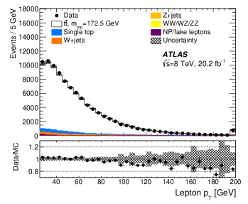
(a) Transverse momentum of the lepton

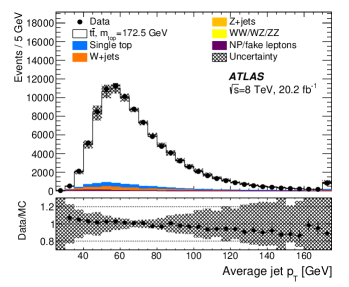
(b) Average transverse momentum of jets

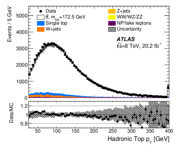
(c) Transverse momentum of the hadronically decaying top quark

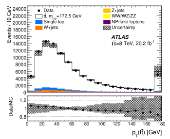
(d) Transverse momentum of the $t\bar{t}$ system

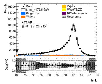
(e) Logarithm of the event likelihood

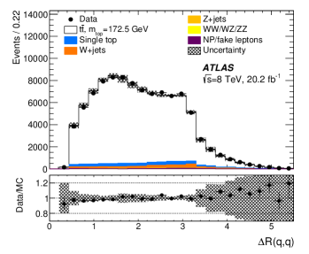
(f) $\Delta R$ of jets from the $W$ boson decay

Figure 1: Distributions for the events passing the preselection. The data are shown together with the signal-plus-background prediction, normalized to the number of events observed in the data. The hatched area is the uncertainty in the prediction as described in the text. The rightmost bin contains all entries with values above the lower edge of this bin, similarly the leftmost bin contains all entries with values below the upper edge of this bin. Figure (a) shows the transverse momentum of the lepton, figure (b) shows the average transverse momentum of the jets, figure (c) shows the transverse momentum of the hadronically decaying top quark, figure (d) shows the transverse momentum of the $t\bar{t}$ system, figure (e) shows the logarithm of the event likelihood of the best permutation and figure (f) shows the distance $\Delta R$ of the two untagged jets $q_{1}$ and $q_{2}$ from the hadronically decaying $W$ boson.

In anticipation of the template parameterization described in Section 7, the following restrictions on the three observables are applied: $125\leq m_{\mathrm{top}}^{\mathrm{reco}}\leq 200\leavevmode\nobreak\ \text{Ge\kern-1.00006ptV}$, $55\leq m_{W}^{\mathrm{reco}}\leq 110\leavevmode\nobreak\ \text{Ge\kern-1.00006ptV}$, and $0.3\leq R_{bq}^{\mathrm{reco}}\leq 3$. Since in this analysis only the best permutation is considered, events that do not pass these requirements are rejected. This removes events in the tails of the three distributions, which are typically poorly reconstructed with small likelihood values and do not contain significant information about $m_{\mathrm{top}}$. The resulting templates have simpler shapes, which are easier to model analytically with fewer parameters. The preselection with these additional requirements is referred to as the standard selection to distinguish it from the boosted decision tree (BDT) optimization for the smallest total uncertainty in $m_{\mathrm{top}}$, discussed in the next section.

6 Multivariate analysis and BDT event selection

For the measurement of $m_{\mathrm{top}}$, the event selection is refined enriching the fraction of events with correct assignments of reconstruction-level objects to their generator-level counterparts which should be better measured and therefore lead to smaller uncertainties. The optimization of the selection is based on the multivariate BDT algorithm implemented in the TMVA package [79]. The reconstruction-level objects are matched to the closest parton-level object within a $\Delta R$ of $0.1$ for electrons and muons and $0.3$ for jets. A matched object is defined as a reconstruction-level object that falls within the relevant $\Delta R$ of any parton-level object of that type, and a correct match means that this generator-level object is the one it originated from. Due to acceptance losses and reconstruction inefficiencies, not all reconstruction-level objects can successfully be matched to their parton-level counterparts. If any object cannot be unambiguously matched, the corresponding event is referred to as unmatched. The efficiency for correctly matched events $\epsilon_{\mathrm{cm}}$ is the fraction of correctly matched events among all the matched events, and the selection purity $\pi_{\mathrm{cm}}$ is the fraction of correctly matched events among all selected events, regardless of whether they could be matched or not.

The BDT algorithm is exploited to enrich the event sample in events that have correct jet-to-parton matching by reducing the remainder, i.e. the sum of incorrectly matched and unmatched events. Using the preselection, the BDT algorithm is trained on the simulated $t\bar{t}$ signal sample with $m_{\mathrm{top}}=172.5$ GeV. Many variables were studied and only those with a separation larger than $0.1\%$ are used in the training. The 13 variables chosen for the final training are given in Table 2. For all input variables to the BDT algorithm, good agreement between the MC predictions and the data is found, as shown in Figures 1(e) and 1(f) for the examples of the likelihood of the chosen permutation and the opening angle $\Delta R$ of the two untagged jets associated with the $W$ boson decay.

Table 2: The input variables to the BDT algorithm sorted by their separation.

Separation	Description
31$\%$	Logarithm of the event likelihood of the best permutation, $\ln L$
13$\%$	$\Delta R$ of the two untagged jets $q_{1}$ and $q_{2}$ from
	the hadronically decaying $W$ boson, $\Delta R(q,q)$
5.0$\%$	$p_{\text{T}}$ of the hadronically decaying $W$ boson
4.3$\%$	$p_{\text{T}}$ of the hadronically decaying top quark
4.2$\%$	Relative event probability of the best permutation
2.0$\%$	$p_{\text{T}}$ of the reconstructed $t\bar{t}$ system
1.7$\%$	$p_{\text{T}}$ of the semi-leptonically decaying top quark
1.2$\%$	Transverse mass of the leptonically decaying $W$ boson
0.3$\%$	$p_{\text{T}}$ of the leptonically decaying $W$ boson
0.3$\%$	Number of jets
0.2$\%$	$\Delta R$ of the reconstructed $b\text{-tagged}$ jets
0.2$\%$	Missing transverse momentum
0.1$\%$	$p_{\text{T}}$ of the lepton

These two variables also have the largest separation for the correctly matched events and the remainder. The corresponding distributions for the two event classes are shown in Figures 2(a) and 2(b).

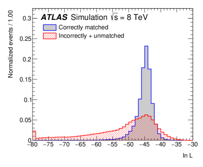
(a) Logarithm of the event likelihood

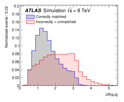
(b) $\Delta R$ of jets from the $W$ boson decay

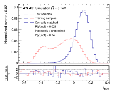
(c) BDT test and training samples

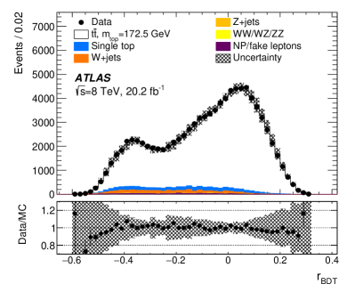
(d) Data-to-simulation comparison for $r_{\mathrm{BDT}}$

Figure 2: Input and results of the BDT training on $t\bar{t}$ signal events for the preselection. Figure (a) shows the logarithm of the event likelihood of the best permutation ($\ln L$) for the correctly matched events and the remainder. Similarly, figure (b) shows the distribution of the $\Delta R$ between the two untagged jets assigned to the $W$ boson decay. Figure (c) shows the distribution of the BDT output ($r_{\mathrm{BDT}}$) for the two classes of events for both the training (histograms) and test samples (points with statistical uncertainties). The compatibility in terms of the $\chi^{2}$ probability is also listed. The distributions peaking at around $r_{\mathrm{BDT}}=0.1$ are for the correctly matched events, the ones to the left are for incorrectly or unmatched events. The ratio figure shows the difference between the number of events in the training and test samples divided by the statistical uncertainty in this difference. Finally, figure (d) shows the comparison of the $r_{\mathrm{BDT}}$ distributions observed in data and MC simulation. The hatched area includes the uncertainties as detailed in the text. The uncertainty bars correspond to the statistical uncertainties in the data.

These figures show a clear separation of the correctly matched events and the remainder. Half the simulation sample is used to train the algorithm and the other half to assess its performance. The significant difference between the distributions of the output value $r_{\mathrm{BDT}}$ of the BDT classifier between the two classes of events in Figure 2(c) shows their efficient separation by the BDT algorithm. In addition, reasonable agreement is found for the $r_{\mathrm{BDT}}$ distributions in the statistically independent test and training samples. The $r_{\mathrm{BDT}}$ distributions in simulation and data in Figure 2(d) agree within the experimental uncertainties. The above findings justify the application of the BDT approach to the data.

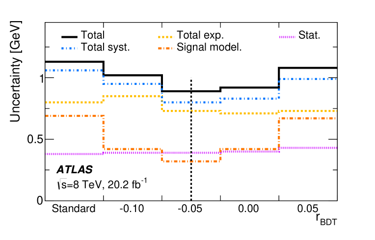
Figure 3: Various classes of $m_{\mathrm{top}}$ uncertainties as a function of the minimum requirement on the BDT output $r_{\mathrm{BDT}}$ and for the standard selection. The total uncertainty (solid line) is the sum in quadrature of the statistical (dotted line) and total systematic uncertainty (short dash-dotted line). The total systematic uncertainty consists of the total experimental (dashed line) and total signal-modelling uncertainty (long dash-dotted line). The uncertainties in the background estimate are included in the total experimental uncertainty. The minimum requirement on $r_{\mathrm{BDT}}$ defining the $\mathrm{BDT}$ selection is indicated by the vertical black dashed line. All uncertainties are included except for the method and the pile-up uncertainties.

The full $m_{\mathrm{top}}$ analysis detailed in Section 8 is performed, except for the evaluation of the small method and pile-up uncertainties described in Section 8, for several minimum requirements on $r_{\mathrm{BDT}}$ in the range of $[-0.10,0.05]$ in steps of 0.05 to find the point with smallest total uncertainty. The total uncertainty in $m_{\mathrm{top}}$ together with the various classes of uncertainty sources as a function of $r_{\mathrm{BDT}}$ evaluated in the $\mathrm{BDT}$ optimization are shown in Figure 3. The minimum requirement $r_{\mathrm{BDT}}=-0.05$ provides the smallest total uncertainty in $m_{\mathrm{top}}$. The resulting numbers of events for this BDT selection are given in Table 1. Compared with the preselection, $\epsilon_{\mathrm{cm}}$ is increased from $0.71$ to $0.82$, albeit at the expense of a significant reduction in the number of selected events. The purity $\pi_{\mathrm{cm}}$ is increased from $0.28$ to $0.41$. In addition, the intrinsic resolution in $m_{\mathrm{top}}$ of the remaining event sample is improved, i.e. the statistical uncertainty in $m_{\mathrm{top}}$ in Figure 3 is almost constant as a function of $r_{\mathrm{BDT}}$; in particular, it does not scale with the square root of the number of events retained. For the signal sample with $m_{\mathrm{top}}=172.5$ GeV, the template fit functions for the standard selection and the $\mathrm{BDT}$ selection, together with their ratios, are shown in Figure 12 in Appendix A. The shape of the signal modelling uncertainty derives from a sum of contributions with different shapes. The curves from the signal Monte Carlo generator and colour reconnection uncertainties decrease, the one from the underlying event uncertainty is flat, the one from the initial- and final-state QCD radiation has a valley similar to the sum of all contributions, and finally the one from the hadronization uncertainty rises.

Some distributions of the observed event kinematics after the $\mathrm{BDT}$ selection are shown in Figure 4. Good agreement between the MC predictions and the data is found, as seen for the preselection in Figure 1. The examples shown are the observed $W$ boson transverse mass for the semi-leptonically decaying top quark in Figure 4(a) and the three observables of the $m_{\mathrm{top}}$ analysis (within the ranges of the template fit) in Figures 4(b)–4(d). The sharp edge observed at 30 GeV in Figure 4(a) originates from the different selection requirements for the $W$ boson transverse mass in the electron+jets and muon+jets final states.

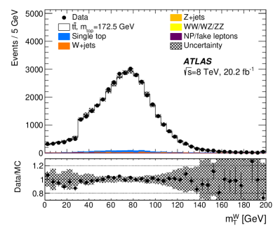
(a) $W$ boson transverse mass

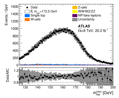
(b) Reconstructed top quark mass

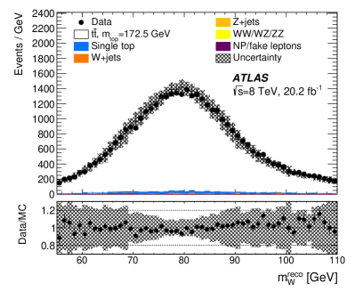
(c) Reconstructed $W$ boson mass

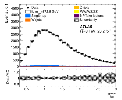
(d) Reconstructed ratio of jet transverse momenta

Figure 4: Distributions for the events passing the BDT selection. The data are shown, together with the signal-plus-background prediction normalized to the number of events observed in the data. The hatched area is the uncertainty in the prediction described in the text. The rightmost bin contains all entries with values above the lower edge of this bin, similarly the leftmost bin contains all entries with values below the upper edge of this bin. Figure (a) shows the $W$ boson transverse mass for the semi-leptonic top quark decay. The remaining figures show the three observables used for the determination of $m_{\mathrm{top}}$, where figure (b) shows the reconstructed top quark mass $m_{\mathrm{top}}^{\mathrm{reco}}$, figure (c) shows the reconstructed invariant mass of the $W$ boson $m_{W}^{\mathrm{reco}}$ and figure (d) shows the reconstructed ratio of jet transverse momenta $R_{bq}^{\mathrm{reco}}$. The three distributions are shown within the ranges of the template fit.

7 Template fit

This analysis uses a three-dimensional template fit technique which determines $m_{\mathrm{top}}$ together with the jet energy scale factors $\mathrm{JSF}$ and $\mathrm{bJSF}$. The aim of the multi-dimensional fit to the data is to measure $m_{\mathrm{top}}$ and, at the same time, to absorb the mean differences between the jet energy scales observed in data and MC simulated events into jet energy scale factors. By using $\mathrm{JSF}$ and $\mathrm{bJSF}$, most of the uncertainties in $m_{\mathrm{top}}$ induced by $\mathrm{JES}$ and $\mathrm{bJES}$ uncertainties are transformed into additional statistical components caused by the higher dimensionality of the fit. This method reduces the total uncertainty in $m_{\mathrm{top}}$ only for sufficiently large data samples. In this case, the sum in quadrature of the additional statistical uncertainty in $m_{\mathrm{top}}$ due to the $\mathrm{JSF}$ (or $\mathrm{bJSF}$) fit and the residual $\mathrm{JES}$-induced (or $\mathrm{bJES}$-induced) systematic uncertainty is smaller than the original $\mathrm{JES}$-induced (or $\mathrm{bJES}$-induced) uncertainty in $m_{\mathrm{top}}$. This situation was already realized for the ${\sqrt{s}}=7$ TeV data analysis [9] and is even more advantageous for the much larger data sample of the ${\sqrt{s}}=8$ TeV data analysis. Since $\mathrm{JSF}$ and $\mathrm{bJSF}$ are global factors, they do not completely absorb the $\mathrm{JES}$ and $\mathrm{bJES}$ uncertainties which have $p_{\text{T}}$- and $\eta$-dependent components.

For simultaneously determining $m_{\mathrm{top}}$, $\mathrm{JSF}$ and $\mathrm{bJSF}$, templates are constructed from the MC samples. Templates of $m_{\mathrm{top}}^{\mathrm{reco}}$ are constructed with several input $m_{\mathrm{top}}$ values used in the range 167.5–177.5 GeV and for the sample at $m_{\mathrm{top}}=172.5$ GeV also with independent input values for $\mathrm{JSF}$ and $\mathrm{bJSF}$ in the range 0.96–1.04 in steps of 0.02. Statistically independent MC samples are used for different input values of $m_{\mathrm{top}}$. The templates with different values of $\mathrm{JSF}$ and $\mathrm{bJSF}$ are constructed by scaling the energies of the jets appropriately. In this procedure, $\mathrm{JSF}$ is applied to all jets, while $\mathrm{bJSF}$ is solely applied to $b\text{-jets}$ according to the generated quark flavour. The scaling is performed after the various correction steps of the jet calibration but before the event selection. This procedure results in different events passing the $\mathrm{BDT}$ selection from one energy scale variation to another. However, many events are in all samples, resulting in a large statistical correlation of the samples with different jet scale factors. Similarly, templates of $m_{W}^{\mathrm{reco}}$ and $R_{bq}^{\mathrm{reco}}$ are constructed with the above listed input values of $m_{\mathrm{top}}$, $\mathrm{JSF}$ and $\mathrm{bJSF}$.

Independent signal templates are derived for the three observables for all $m_{\mathrm{top}}$-dependent samples, consisting of the $t\bar{t}$ signal events and single-top-quark production events. This procedure is adopted because single-top-quark production carries information about the top quark mass, and in this way, $m_{\mathrm{top}}$-independent background templates can be used. The signal templates are simultaneously fitted to the sum of a Gaussian and two Landau functions for $m_{\mathrm{top}}^{\mathrm{reco}}$, to the sum of two Gaussian functions for $m_{W}^{\mathrm{reco}}$ and to the sum of two Gaussian and one Landau function for $R_{bq}^{\mathrm{reco}}$. This set of functions leads to an unbiased estimate of $m_{\mathrm{top}}$, but is not unique. For the background, the $m_{\mathrm{top}}^{\mathrm{reco}}$ distribution is fitted to a Landau function, while both the $m_{W}^{\mathrm{reco}}$ and the $R_{bq}^{\mathrm{reco}}$ distributions are fitted to the sum of two Gaussian functions.

In Figures 5(a)–5(c), the sensitivity of $m_{\mathrm{top}}^{\mathrm{reco}}$ to the fit parameters $m_{\mathrm{top}}$, $\mathrm{JSF}$ and $\mathrm{bJSF}$ is shown by the superposition of the signal templates and their fits for three input values per varied parameter. In a similar way, the sensitivity of $m_{W}^{\mathrm{reco}}$ to $\mathrm{JSF}$ is shown in Figure 5(d). The dependences of $m_{W}^{\mathrm{reco}}$ on the input values of $m_{\mathrm{top}}$ and $\mathrm{bJSF}$ are negligible and are not shown. Consequently, to increase the size of the simulation sample, the fit is performed on the sum of the $m_{W}^{\mathrm{reco}}$ distributions of the samples with different input top quark masses. Finally, the sensitivity of $R_{bq}^{\mathrm{reco}}$ to the input values of $m_{\mathrm{top}}$ and $\mathrm{bJSF}$ is shown in Figures 5(e) and 5(f). The dependence of $R_{bq}^{\mathrm{reco}}$ on $\mathrm{JSF}$ (not shown) is much weaker than the dependence on $\mathrm{bJSF}$.

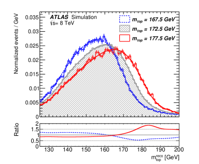
(a) $m_{\mathrm{top}}^{\mathrm{reco}}$ with three input $m_{\mathrm{top}}$

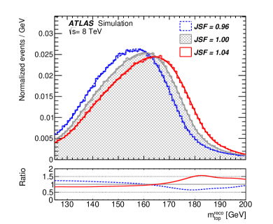
(b) $m_{\mathrm{top}}^{\mathrm{reco}}$ with three input $\mathrm{JSF}$

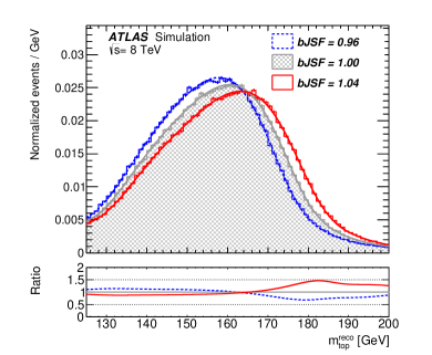
(c) $m_{\mathrm{top}}^{\mathrm{reco}}$ with three input $\mathrm{bJSF}$

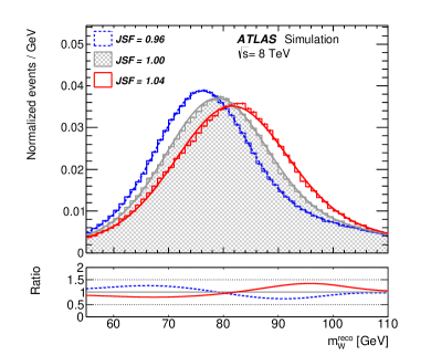
(d) $m_{W}^{\mathrm{reco}}$ with three input $\mathrm{JSF}$

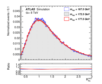
(e) $R_{bq}^{\mathrm{reco}}$ with three input $m_{\mathrm{top}}$

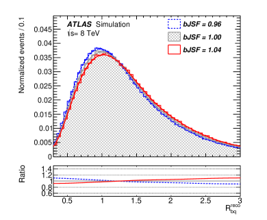
(f) $R_{bq}^{\mathrm{reco}}$ with three input $\mathrm{bJSF}$

Figure 5: Template parameterizations for signal events, composed of $t\bar{t}$ and single-top-quark production events. Figures (a)–(c) show the sensitivity of $m_{\mathrm{top}}^{\mathrm{reco}}$ to $m_{\mathrm{top}}$, $\mathrm{JSF}$ and $\mathrm{bJSF}$, figure (d) shows the sensitivity of $m_{W}^{\mathrm{reco}}$ to $\mathrm{JSF}$ and figures (e) and (f) show the sensitivity of $R_{bq}^{\mathrm{reco}}$ to $m_{\mathrm{top}}$ and $\mathrm{bJSF}$. Each template is overlaid with the corresponding probability density function from the combined fit to all templates described in the text. The ratios shown are calculated relative to the probability density function of the central sample with $m_{\mathrm{top}}=172.5$ GeV, $\mathrm{JSF}=1$ and $\mathrm{bJSF}=1$.

For the signal, the parameters of the fitting functions for $m_{\mathrm{top}}^{\mathrm{reco}}$ depend linearly on $m_{\mathrm{top}}$, $\mathrm{JSF}$ and $\mathrm{bJSF}$. The parameters of the fitting functions for $m_{W}^{\mathrm{reco}}$ depend linearly on $\mathrm{JSF}$. Finally, the parameters of the fitting functions for $R_{bq}^{\mathrm{reco}}$ depend linearly on $m_{\mathrm{top}}$, $\mathrm{JSF}$ and $\mathrm{bJSF}$. For the background, the dependences of the parameters of the fitting functions are identical to those for the signal, except that they do not depend on $m_{\mathrm{top}}$ and that those for $R_{bq}^{\mathrm{reco}}$ do not depend on $\mathrm{JSF}$.

Signal and background probability density functions $P_{\mathrm{top}}^{\mathrm{sig}}$ and $P_{\mathrm{top}}^{\mathrm{bkg}}$ for the $m_{\mathrm{top}}^{\mathrm{reco}}$, $m_{W}^{\mathrm{reco}}$ and $R_{bq}^{\mathrm{reco}}$ distributions are used in an unbinned likelihood fit to the data for all events, $i=1,\dots N$. The likelihood function maximized is

$$L_{\mathrm{shape}}^{\ell\mathrm{+jets}}(m_{\mathrm{top}},\mathrm{JSF},\mathrm{bJSF},f_{\mathrm{bkg}}) =\prod_{i=1}^{N}P_{\mathrm{top}}(m_{\mathrm{top}}^{\mathrm{reco},i}\,|\,m_{\mathrm{top}},\mathrm{JSF},\mathrm{bJSF},f_{\mathrm{bkg}})$$

$$\quad\quad\times\,P_{W}(m_{W}^{\mathrm{reco},i}\,|\,\mathrm{JSF},f_{\mathrm{bkg}})$$

$$\quad\quad\times\,P_{R_{bq}}(R_{bq}^{\mathrm{reco},i}\,|\,m_{\mathrm{top}},\mathrm{JSF},\mathrm{bJSF},f_{\mathrm{bkg}}),$$ (1)

with

$$P_{\mathrm{top}}(m_{\mathrm{top}}^{\mathrm{reco},i}\,|\,m_{\mathrm{top}},\mathrm{JSF},\mathrm{bJSF},f_{\mathrm{bkg}}) =(1-f_{\mathrm{bkg}})\cdot P_{\mathrm{top}}^{\mathrm{sig}}(m_{\mathrm{top}}^{\mathrm{reco},i}\,|\,m_{\mathrm{top}},\mathrm{JSF},\mathrm{bJSF})+$$

$$\quad\quad\quad\,\,\,f_{\mathrm{bkg}}\cdot P_{\mathrm{top}}^{\mathrm{bkg}}(m_{\mathrm{top}}^{\mathrm{reco},i}\,|\,\mathrm{JSF},\mathrm{bJSF})\,\,,$$

$$P_{W}(m_{W}^{\mathrm{reco},i}\,|\,\mathrm{JSF},f_{\mathrm{bkg}}) =(1-f_{\mathrm{bkg}})\cdot P_{W}^{\mathrm{sig}}(m_{W}^{\mathrm{reco},i}\,|\,\mathrm{JSF})+$$

$$\quad\quad\quad\,\,\,f_{\mathrm{bkg}}\cdot P_{W}^{\mathrm{bkg}}(m_{W}^{\mathrm{reco},i}\,|\,\mathrm{JSF})\,\,,\textrm{ and}$$

$$P_{R_{bq}}(R_{bq}^{\mathrm{reco},i}\,|\,m_{\mathrm{top}},\mathrm{JSF},\mathrm{bJSF},f_{\mathrm{bkg}}) =(1-f_{\mathrm{bkg}})\cdot P_{R_{bq}}^{\mathrm{sig}}(R_{bq}^{\mathrm{reco},i}\,|\,m_{\mathrm{top}},\mathrm{JSF},\mathrm{bJSF})+$$

$$\quad\quad\quad\,\,\,f_{\mathrm{bkg}}\cdot P_{R_{bq}}^{\mathrm{bkg}}(R_{bq}^{\mathrm{reco},i}\,|\,\mathrm{bJSF})\,\,$$

where the fraction of background events is denoted by $f_{\mathrm{bkg}}$. The parameters determined by the fit are $m_{\mathrm{top}}$, $\mathrm{JSF}$ and $\mathrm{bJSF}$, while $f_{\mathrm{bkg}}$ is fixed to its expectation shown in Table 1. It was verified that the correlations between $m_{\mathrm{top}}^{\mathrm{reco}}$, $m_{W}^{\mathrm{reco}}$ and $R_{bq}^{\mathrm{reco}}$ of $\rho(m_{\mathrm{top}}^{\mathrm{reco}},m_{W}^{\mathrm{reco}})=0.05$, $\rho(m_{\mathrm{top}}^{\mathrm{reco}},R_{bq}^{\mathrm{reco}})=0.18$, and $\rho(m_{W}^{\mathrm{reco}},R_{bq}^{\mathrm{reco}})=-0.13$, are small enough that formulating the likelihood in Eq. (1) as a product of three one-dimensional likelihoods does not bias the result.

Pseudo-experiments are used to verify the internal consistency of the fitting procedure and to obtain the expected statistical uncertainty for the data. For each set of parameter values, $500$ pseudo-experiments are performed, each corresponding to the integrated luminosity of the data. To retain the correlation of the three observables for the three-dimensional fit, individual events are used. Because this exceeds the number of available MC events, results are corrected for oversampling [80]. The results of pseudo-experiments for different input values of $m_{\mathrm{top}}$ are obtained from statistically independent samples, while the results for different $\mathrm{JSF}$ and $\mathrm{bJSF}$ are obtained from statistically correlated samples as explained above. For each fitted quantity and each variation of input parameters, the residual, i.e. the difference between the input value and the value obtained by the fit, is compatible with zero. The three expected statistical uncertainties are

$$\sigma_{\mathrm{stat}}(m_{\mathrm{top}}) ={} 0.389 {}\pm{} 0.004\leavevmode\nobreak\ \text{Ge\kern-1.00006ptV},$$

$$\sigma_{\mathrm{stat}}(\mathrm{JSF}) ={} 0.00115 {}\pm{} 0.00001\,,\textrm{ and}$$

$$\sigma_{\mathrm{stat}}(\mathrm{bJSF}) ={} 0.0046 {}\pm{} 0.0001\,,$$

where the values quoted are the mean and RMS of the distribution of the statistical uncertainties in the fitted quantities from pseudo-experiments. The widths of the pull distributions are below unity for $m_{\mathrm{top}}$ and the two jet scale factors, which results in an overestimation of the uncertainty in $m_{\mathrm{top}}$ of up to 7$\%$. Since this leads to a conservative estimate of the uncertainty in $m_{\mathrm{top}}$, no attempts to mitigate this feature are made.

8 Uncertainties affecting the $m_{\mathrm{top}}$ determination

Table 3: Systematic uncertainties in $m_{\mathrm{top}}$. The measured values of $m_{\mathrm{top}}$ are given together with the statistical and systematic uncertainties in GeV for the standard and the BDT event selections. For comparison, the result in the $t\bar{t}\to\mathrm{lepton+jets}$ channel at ${\sqrt{s}}=7$ TeV from LABEL:\cite[cite]{[\@@bibref{}{TOPQ-2013-02}{}{}]} is also listed. For each systematic uncertainty listed, the first value corresponds to the uncertainty in $m_{\mathrm{top}}$, and the second to the statistical precision in this uncertainty. An integer value of zero means that the corresponding uncertainty is negligible and therefore not evaluated. Statistical uncertainties quoted as 0.00 are smaller than 0.005. The statistical uncertainty in the total systematic uncertainty is calculated from uncertainty propagation. The last line refers to the sum in quadrature of the statistical and systematic uncertainties.

	${\sqrt{s}}=7$ TeV	${\sqrt{s}}=8$ TeV
Event selection	Standard	Standard	BDT
$m_{\mathrm{top}}$ result [GeV]	$172.33$	$171.90$	$172.08$
Statistics	$0.75$	$0.38$	$0.39$
– Stat. comp. ($m_{\mathrm{top}}$)	$0.23$	$0.12$	$0.11$
– Stat. comp. ($\mathrm{JSF}$)	$0.25$	$0.11$	$0.11$
– Stat. comp. ($\mathrm{bJSF}$)	$0.67$	$0.34$	$0.35$
Method	0.11 $\pm$ 0.10	0.04 $\pm$ 0.11	0.13 $\pm$ 0.11
Signal Monte Carlo generator	0.22 $\pm$ 0.21	0.50 $\pm$ 0.17	0.16 $\pm$ 0.17
Hadronization	0.18 $\pm$ 0.12	0.05 $\pm$ 0.10	0.15 $\pm$ 0.10
Initial- and final-state QCD radiation	0.32 $\pm$ 0.06	0.28 $\pm$ 0.11	0.08 $\pm$ 0.11
Underlying event	0.15 $\pm$ 0.07	0.08 $\pm$ 0.15	0.08 $\pm$ 0.15
Colour reconnection	0.11 $\pm$ 0.07	0.37 $\pm$ 0.15	0.19 $\pm$ 0.15
Parton distribution function	0.25 $\pm$ 0.00	0.08 $\pm$ 0.00	0.09 $\pm$ 0.00
Background normalization	0.10 $\pm$ 0.00	0.04 $\pm$ 0.00	0.08 $\pm$ 0.00
$W$+jets shape	0.29 $\pm$ 0.00	0.05 $\pm$ 0.00	0.11 $\pm$ 0.00
Fake leptons shape	0.05 $\pm$ 0.00	0	0
Jet energy scale	0.58 $\pm$ 0.11	0.63 $\pm$ 0.02	0.54 $\pm$ 0.02
Relative $b$-to-light-jet energy scale	0.06 $\pm$ 0.03	0.05 $\pm$ 0.01	0.03 $\pm$ 0.01
Jet energy resolution	0.22 $\pm$ 0.11	0.23 $\pm$ 0.03	0.20 $\pm$ 0.04
Jet reconstruction efficiency	0.12 $\pm$ 0.00	0.04 $\pm$ 0.01	0.02 $\pm$ 0.01
Jet vertex fraction	0.01 $\pm$ 0.00	0.13 $\pm$ 0.01	0.09 $\pm$ 0.01
$b\text{-tagging}$	0.50 $\pm$ 0.00	0.37 $\pm$ 0.00	0.38 $\pm$ 0.00
Leptons	0.04 $\pm$ 0.00	0.16 $\pm$ 0.01	0.16 $\pm$ 0.01
Missing transverse momentum	0.15 $\pm$ 0.04	0.08 $\pm$ 0.01	0.05 $\pm$ 0.01
Pile-up	0.02 $\pm$ 0.01	0.14 $\pm$ 0.01	0.15 $\pm$ 0.01
Total systematic uncertainty	$1.04$ $\pm$ $0.08$	$1.07$ $\pm$ $0.10$	$0.82$ $\pm$ $0.06$
Total	$1.28$ $\pm$ $0.08$	$1.13$ $\pm$ $0.10$	$0.91$ $\pm$ $0.06$

This section focuses on the treatment of uncertainty sources of a systematic nature. The same systematic uncertainty sources as in LABEL:\cite[cite]{[\@@bibref{}{TOPQ-2013-02}{}{}]} are investigated. If possible, the corresponding uncertainty in $m_{\mathrm{top}}$ is evaluated by varying the respective quantities by $\pm 1\sigma$ from their default values, constructing the corresponding event sample and measuring the average $m_{\mathrm{top}}$ change relative to the result from the nominal MC sample with $500$ pseudo-experiments each, drawn from the full MC sample. In the absence of a $\pm 1\sigma$ variation, e.g. for the evaluation of the uncertainty induced by the choice of signal MC generator, the full observed difference is assigned as a symmetric systematic uncertainty and further treated as a variation equivalent to a $\pm 1\sigma$ variation. Wherever a $\pm 1\sigma$ variation can be performed, half the observed difference between the $+1\sigma$ and $-1\sigma$ variation in $m_{\mathrm{top}}$ is assigned as an uncertainty if the $m_{\mathrm{top}}$ values obtained from the variations lie on opposite sides of the nominal result. If they lie on the same side, the maximum observed difference is taken as a symmetric systematic uncertainty. Since the systematic uncertainties are derived from simulation or data samples with limited numbers of events, all systematic uncertainties have a corresponding statistical uncertainty, which is calculated taking into account the statistical correlation of the considered samples, as explained in Section 8.5. The statistical uncertainty in the total systematic uncertainty is dominated by the limited sizes of the simulation samples. The resulting systematic uncertainties are given in Table 3 independent of their statistical significance. Further information is given in Tables 8–12 in Appendix A. This approach follows the suggestion in LABEL:\cite[cite]{[\@@bibref{}{Barlow:2002yb}{}{}]} and relies on the fact that, given a large enough number of considered uncertainty sources, statistical fluctuations average out. The uncertainty sources are designed to be uncorrelated with each other, and thus the total uncertainty is taken as the sum in quadrature of uncertainties from all sources. The individual uncertainties are compared in Table 3 for three cases: the standard selection for the ${\sqrt{s}}=7$ TeV [9] and 8 TeV data and the $\mathrm{BDT}$ selection for ${\sqrt{s}}=8$ TeV data. Many uncertainties in $m_{\mathrm{top}}$ obtained with the standard selection at the two centre-of-mass energies agree within their statistical uncertainties such that the resulting total systematic uncertainties are almost identical. Consequently, repeating the ${\sqrt{s}}=7$ TeV analysis on ${\sqrt{s}}=8$ TeV data would have only improved the statistical precision. The picture changes when comparing the uncertainties in ${\sqrt{s}}=8$ TeV data for the standard selection and the $\mathrm{BDT}$ selection. In general, the experimental uncertainties change only slightly, with the largest reduction observed for the JES uncertainty. In contrast, a large improvement comes from the reduced uncertainties in the modelling of the $t\bar{t}$ signal processes as shown in Table 3. This, together with the improved intrinsic resolution in $m_{\mathrm{top}}$, more than compensates for the small loss in precision caused by the increased statistical uncertainty. The individual sources of systematic uncertainties and the evaluation of their effect on $m_{\mathrm{top}}$ are described in the following.

8.1 Statistics and method calibration

Uncertainties related to statistical effects and the method calibration are discussed here.

Statistical:

The quoted statistical uncertainty consists of three parts: a purely statistical component in $m_{\mathrm{top}}$ and the contributions stemming from the simultaneous determination of $\mathrm{JSF}$ and $\mathrm{bJSF}$. The purely statistical component in $m_{\mathrm{top}}$ is obtained from a one-dimensional template method exploiting only the $m_{\mathrm{top}}^{\mathrm{reco}}$ observable, while fixing the values of $\mathrm{JSF}$ and $\mathrm{bJSF}$ to the results of the three-dimensional analysis. The contribution to the statistical uncertainty in the fitted parameters due to the simultaneous fit of $m_{\mathrm{top}}$ and $\mathrm{JSF}$ is estimated as the difference in quadrature between the statistical uncertainty in a two-dimensional fit to $m_{\mathrm{top}}^{\mathrm{reco}}$ and $m_{W}^{\mathrm{reco}}$ while fixing the value of $\mathrm{bJSF}$ and the one-dimensional fit to the data described above. Analogously, the contribution of the statistical uncertainty due to the simultaneous fit of $m_{\mathrm{top}}$ together with $\mathrm{JSF}$ and $\mathrm{bJSF}$ is defined as the difference in quadrature between the statistical uncertainties obtained in the three-dimensional and the two-dimensional fits to the data. This separation allows a comparison of the statistical sensitivities of the $m_{\mathrm{top}}$ estimator used in this analysis, to those of analyses exploiting a different number of observables in the fit. In addition, the sensitivity of the estimators to the global jet energy scale factors can be compared directly. These uncertainties are treated as uncorrelated uncertainties in $m_{\mathrm{top}}$ combinations. Together with the systematic uncertainty in the residual jet energy scale uncertainties discussed below, they directly replace the uncertainty in $m_{\mathrm{top}}$ from the jet energy scale variations present without the in situ determination.

Method:

The residual difference between fitted and generated $m_{\mathrm{top}}$ when analysing a template from a MC sample reflects the potential bias of the method. Consequently, the largest observed fitted $m_{\mathrm{top}}$ residual and the largest observed statistical uncertainty in this quantity, in any of the five signal samples with different assumed values of $m_{\mathrm{top}}$, is assigned as the method calibration uncertainty and its corresponding statistical uncertainty, respectively. This also covers effects from limited numbers of simulated events in the templates and potential deficiencies in the template parameterizations.

8.2 Modelling of signal processes

The modelling of $t\bar{t}\to\mathrm{lepton+jets}$ events incorporates a number of processes that have to be accurately described, resulting in systematic effects, ranging from the $t\bar{t}$ production to the hadronization of the showered objects.

Thanks to the restrictive event-selection requirements, the contribution of non-$t\bar{t}$ processes, comprising the single-top-quark process and the various background processes, is very low. The systematic uncertainty in $m_{\mathrm{top}}$ from the uncertainty in the single-top-quark normalization is estimated from the corresponding uncertainty in the theoretical cross-section given in Section 3. The resulting systematic uncertainty is small compared with the systematic uncertainty in the $t\bar{t}$ production and is consequently neglected. For the modelling of the signal processes, the consequence of including single-top-quark variations in the uncertainty evaluation was investigated for various uncertainty sources and found to be negligible. Therefore, the single-top-quark variations are not included in the determination of the signal event uncertainties.

Signal Monte Carlo generator:

The full observed difference in fitted $m_{\mathrm{top}}$ between the event samples produced with the Powheg-Box and MC@NLO [82, 83] programs is quoted as a systematic uncertainty. For the renormalization and factorization scales the Powheg-Box sample uses the function given in Section 3, while the MC@NLO sample uses $\mu_{\mathrm{R,F}}=\sqrt{m_{\mathrm{top}}^{2}+0.5(p_{{\mathrm{T}},t}^{2}+p_{{\mathrm{T}},\bar{t}}^{2})}$. Both samples are generated with a top quark mass of $m_{\mathrm{top}}=172.5$ GeV with the CT10 PDFs in the matrix-element calculation and use the Herwig and Jimmy programs with the ATLAS AUET2 tune [47].

Hadronization:

To cover the choice of parton shower and hadronization models, samples produced with the Powheg-Box program are showered with either the Pythia6 program using the P2011C tune or the Herwig and Jimmy programs using the ATLAS AUET2 tune. This includes different approaches in shower modelling, such as using a $p_{\text{T}}$-ordered parton showering in the Pythia program or angular-ordered parton showering in the Herwig program, the different parton shower matching scales, as well as fragmentation functions and hadronization models, such as choosing the Lund string model [84, 85] implemented in the Pythia program or the cluster fragmentation model [86] used in the Herwig program. The full observed difference between the samples is quoted as a systematic uncertainty.

As shown in Figure 1, the distributions of transverse momenta in data are slightly softer than those in the Powheg+Pythia MC simulation samples. Similarly to what was observed in the $t\bar{t}\to\mathrm{dilepton}$ channel for the $p_{\mathrm{T},\ell b}$ distribution, in the $t\bar{t}\to\mathrm{lepton+jets}$ channel the Powheg+Herwig sample is much closer to the data for several distributions of transverse momenta. The $p_{\mathrm{T,had}}$ distribution is much better described by the Powheg+Herwig sample as was also observed in Ref. [78]. In addition, but to a lesser extent, the MC@NLO sample used to assess the signal Monte Carlo generator uncertainty and the samples to assess the initial- and final-state QCD radiation uncertainty discussed next also lead to a softer distribution in simulation. Given this, the observed difference in the $p_{\mathrm{T,had}}$ distribution is covered by a combination of the signal-modelling uncertainties given in Table 3.

Despite the fact that the $\mathrm{JES}$ and $\mathrm{bJES}$ are estimated independently using dijet and other non-$t\bar{t}$ samples [63], some double-counting of hadronization-uncertainty-induced uncertainties in the $\mathrm{JES}$ and $m_{\mathrm{top}}$ cannot be excluded. This was investigated closely for the ATLAS top quark mass measurement in the $t\bar{t}\to\mathrm{lepton+jets}$ channel at ${\sqrt{s}}=7$ TeV. The results in LABEL:\cite[cite]{[\@@bibref{}{ATL-PHYS-PUB-2015-042}{}{}]} revealed that the amount of double-counting of $\mathrm{JES}$ and hadronization effects for the $t\bar{t}\to\mathrm{lepton+jets}$ channel is small.

Initial- and final-state QCD radiation (ISR/FSR):

ISR/FSR leads to a higher jet multiplicity and different jet energies than the hard process, which affects the distributions of the three observables. The uncertainties due to ISR/FSR modelling are estimated with samples generated with the Powheg-Box program interfaced to the Pythia6 program for which the parameters of the generation are varied to span the ranges compatible with the results of measurements of $t\bar{t}$ production in association with jets [88, 89, 90]. This uncertainty is evaluated by comparing two dedicated samples that differ in several parameters, namely the QCD scale $\Lambda_{\mathrm{QCD}}$, the transverse momentum scale for space-like parton-shower evolution $Q^{2}_{\mathrm{max}}$, the $h_{\mathrm{damp}}$ parameter [91] and the P2012 RadLo and RadHi tunes [30]. In LABEL:\cite[cite]{[\@@bibref{}{ATL-PHYS-PUB-2015-002}{}{}]}, it was shown that a number of final-state distributions are better accounted for by the Powheg+Pythia samples with $h_{\mathrm{damp}}=m_{\mathrm{top}}$. Therefore, these samples are used for evaluating this uncertainty, taking half the observed difference between the up variation and the down variation sample. Because the parameterizations for the template fit to data are obtained from Powheg+Pythia samples using $h_{\mathrm{damp}}=\infty$, it was verified that, considering the method uncertainty quoted in Table 3, applying the same functions to the $h_{\mathrm{damp}}=m_{\mathrm{top}}$ samples leads to a result compatible with the input top quark mass.

Underlying event:

To reduce statistical fluctuations in the evaluation of this systematic uncertainty, the difference in underlying-event modelling is assessed by comparing a pair of Powheg-Box samples based on the same partonic events generated with the CT10 PDFs. A sample with the P2012 tune is compared with a sample with the P2012 mpiHi tune [30], with both tunes using the same CTEQ6L1 PDFs [92] for parton showering and hadronization. The Perugia 2012 mpiHi tune provides more semi-hard multiple parton interactions and is used for this comparison with identical colour reconnection parameters in both tunes. The full observed difference is assigned as a systematic uncertainty.

Colour reconnection:

This systematic uncertainty is estimated using a pair of samples with the same partonic events as for the underlying-event uncertainty evaluation but with the P2012 tune and the P2012 loCR tune [30] for parton showering and hadronization. The full observed difference is assigned as a systematic uncertainty.

Parton distribution function (PDF):

The PDF systematic uncertainty is the sum in quadrature of three contributions. These are the sum in quadrature of the differences in fitted $m_{\mathrm{top}}$ for the 26 eigenvector variations of the CT10 PDF and two differences in $m_{\mathrm{top}}$ obtained from reweighting the central CT10 PDF set to the MSTW2008 PDF [39] and the NNPDF2.3 PDF [42].

8.3 Modelling of background processes

Uncertainties in the modelling of the background processes are taken into account by variations of the corresponding normalizations and shapes of the distributions.

Background normalization:

The normalizations are varied for the data-driven background estimates according to their uncertainties. For the negligible contribution from diboson production, no normalization uncertainty is evaluated.

Background shape:

For the $W$+jets background, the shape uncertainty is evaluated from the variation of the heavy-flavour fractions. The corresponding uncertainty is small. Given the very small contribution from $Z$+jets, diboson and NP/fake-lepton backgrounds, no shape uncertainty is evaluated for these background sources.

8.4 Detector modelling

The level of understanding of the detector response and of the particle interactions therein is reflected in numerous systematic uncertainties.

Jet energy scale (JES):

The $\mathrm{JES}$ is measured with a relative precision of about $1\%$ to $4\%$, typically falling with increasing jet $p_{\text{T}}$ and rising with increasing jet $|\eta|$ [93, 94]. The total $\mathrm{JES}$ uncertainty consists of more than 60 subcomponents originating from the various steps in the jet calibration. The number of these nuisance parameters is reduced with a matrix diagonalization of the full $\mathrm{JES}$ covariance matrix including all nuisance parameters for a given category of the $\mathrm{JES}$ uncertainty components.

The analyses of ${\sqrt{s}}=7$ TeV and ${\sqrt{s}}=8$ TeV data make use of the EM+JES and LCW+GSC [93] jet calibrations, respectively. The two calibrations feature different sets of nuisance parameters, and the LCW+GSC calibration generally has smaller uncertainties than the EM+JES calibration. While the pile-up correction for the jet calibration for ${\sqrt{s}}=7$ TeV data only depends on the number of primary vertices ($n_{\mathrm{vtx}}$) and the mean number of interactions per bunch crossing ($\mu$), a pile-up subtraction method based on jet area is introduced for the ${\sqrt{s}}=8$ TeV data. Terms to account for uncertainties in the pile-up estimation are added. They depend on the jet $p_{\text{T}}$ and the local transverse momentum density. In addition, the punch-through uncertainty, i.e. an uncertainty for jets that penetrate through to the muon spectrometer, is added. The final reduced number of nuisance parameters for the ${\sqrt{s}}=8$ TeV analysis is 25. The JES-uncertainty-induced uncertainty in $m_{\mathrm{top}}$ is the dominant systematic uncertainty for all results shown in Table 3. When only a one-dimensional fit to $m_{\mathrm{top}}^{\mathrm{reco}}$ or a two-dimensional fit to $m_{\mathrm{top}}^{\mathrm{reco}}$ and $m_{W}^{\mathrm{reco}}$ is done, this uncertainty is $0.99$ GeV or $0.74$ GeV, respectively.

Relative $b$-to-light-jet energy scale (bJES):

The $\mathrm{bJES}$ uncertainty is an additional uncertainty for the remaining differences between $b\text{-jets}$ and light-jets after the global $\mathrm{JES}$ is applied, and therefore the corresponding uncertainty is uncorrelated with the $\mathrm{JES}$ uncertainty. An additional uncertainty of $0.2\%$ to $1.2\%$ is assigned to $b\text{-jets}$, with the lowest uncertainty for $b\text{-jets}$ with high transverse momenta [63]. Due to the determination of $\mathrm{bJSF}$, the $\mathrm{bJES}$ uncertainty leads to a very small contribution to the uncertainty in $m_{\mathrm{top}}$ in Table 3. However, performing only a two-dimensional fit to $m_{\mathrm{top}}^{\mathrm{reco}}$ and $m_{W}^{\mathrm{reco}}$ would result in an uncertainty of $0.47$ GeV from this source.

Jet energy resolution (JER):

The JER uncertainty is determined following an eigenvector decomposition strategy similar to the $\mathrm{JES}$ systematic uncertainties [93, 94]. The 11 components take into account various effects evaluated from simulation-to-data comparisons including calorimeter noise terms in the forward region. The corresponding uncertainty in $m_{\mathrm{top}}$ is the sum in quadrature of the components of the eigenvector decomposition.

Jet reconstruction efficiency (JRE):

This uncertainty is evaluated by randomly removing $0.23\%$ of the jets with $p_{\text{T}}<30$ GeV from the simulated events prior to the event selection to reflect the precision with which the data-to-simulation JRE ratio is known [62]. The fitted $m_{\mathrm{top}}$ difference between the varied sample and the nominal sample is taken as a systematic uncertainty.

Jet vertex fraction (JVF):

When summing the scalar $p_{\text{T}}$ of all tracks in a jet, the JVF is the fraction contributed by tracks originating at the primary vertex. The uncertainty in $m_{\mathrm{top}}$ is evaluated by varying the requirement on the JVF within its uncertainty [65].

$b\text{-tagging}$:

Mismodelling of the $b\text{-tagging}$ efficiency and mistag rate is accounted for by the application of jet-specific scale factors to simulated events [66]. These scale factors depend on jet $p_{\text{T}}$, jet $\eta$ and the underlying quark flavour. The ones used in this analysis are derived from dijet and $t\bar{t}\to\mathrm{dilepton}$ [66] events. They are the same as those used for the measurement of $m_{\mathrm{top}}$ in the $t\bar{t}\to\mathrm{dilepton}$ channel [14]. Similarly to the $\mathrm{JES}$ uncertainties, the $b\text{-tagging}$ uncertainties are estimated by using an eigenvector approach, based on the $b\text{-tagging}$ calibration analysis [66, 67, 68]. They include the uncertainties in the $b\text{-tagging}$, $c/\tau$-tagging and mistagging scale factors. This uncertainty in $m_{\mathrm{top}}$ is derived by varying the scale factors within their uncertainties and adding the resulting fitted differences in quadrature. In this procedure, uncertainties that are considered both in the $b\text{-tagging}$ calibration and as separate sources in the $m_{\mathrm{top}}$ analysis are taken into account simultaneously by applying the corresponding varied $b\text{-tagging}$ scale factors together with the varied sample when assessing the corresponding uncertainty in $m_{\mathrm{top}}$. The final uncertainty is the sum in quadrature of these independent components. Compared with the result from ${\sqrt{s}}=7$ TeV data, this uncertainty is reduced by about one third for both the standard and $\mathrm{BDT}$ event selections in accordance with the improvements made in the calibrations of the $b\text{-tagging}$ algorithm [66, 67].

Leptons:

The lepton uncertainties are related to the electron energy or muon momentum scale and resolution, as well as trigger, isolation and identification efficiencies. These are measured very precisely in high-purity $J/\psi\to\ell^{+}\ell^{-}$ and $Z\to\ell^{+}\ell^{-}$ data [95, 58, 57]. For each component, the corresponding uncertainty is propagated to the analysis by variation of the respective quantity. The changes are propagated to the $E_{\text{T}}^{\text{miss}}$ as well.

Missing transverse momentum:

The remaining contribution to the missing-transverse-momentum uncertainty stems from the uncertainties in calorimeter-cell energies associated with low-$p_{\text{T}}$ jets ($7\leavevmode\nobreak\ \text{Ge\kern-1.00006ptV}<p_{\text{T}}<20\leavevmode\nobreak\ \text{Ge\kern-1.00006ptV}$) without any corresponding reconstructed physics object or from pile-up interactions. They are accounted for as described in LABEL:\cite[cite]{[\@@bibref{}{PERF-2014-04}{}{}]}. The corresponding uncertainty in $m_{\mathrm{top}}$ is small.

Pile-up:

Besides the component treated in the $\mathrm{JES}$ uncertainty, the residual dependence of the fitted $m_{\mathrm{top}}$ on the amount of pile-up activity and a possible mismodelling of pile-up in MC simulation is determined. For this, the $m_{\mathrm{top}}$ dependence in bins of $n_{\mathrm{vtx}}$ and $\mu$ is determined for data and MC simulated events. Within the statistical uncertainties, the slopes of the linear dependences of $m_{\mathrm{top}}$ observed in data and predicted by the MC simulation are compatible. The same is true for $\mathrm{JSF}$ and $\mathrm{bJSF}$. The final effect on the measurement is assessed by a convolution of the linear dependence with the respective $n_{\mathrm{vtx}}$ and $\mu$ distributions observed for data and MC simulated events. The maximum of the $n_{\mathrm{vtx}}$ and $\mu$ effects is assigned as an uncertainty due to pile-up. The pile-up conditions differ between the ${\sqrt{s}}=7$ and 8 TeV data. For the BDT selection of ${\sqrt{s}}=8$ TeV data used here, the average of the mean number of inelastic $pp$ interactions per bunch crossing is $\langle\mu\rangle=20.3$ and the average number of reconstructed primary vertices is about $n_{\mathrm{vtx}}=9.4$, to be compared with $\langle\mu\rangle=8.8$ and $n_{\mathrm{vtx}}=7.0$ for ${\sqrt{s}}=7$ TeV data [65]. The corresponding uncertainty is somewhat larger than for ${\sqrt{s}}=7$ TeV data but still small.

8.5 Statistical precision of systematic uncertainties

The systematic uncertainties quoted in Table 3 carry statistical uncertainties themselves. In view of a combination with other measurements, the statistical precision $\sigma$ from a comparison of two samples (1 and 2) is determined for each uncertainty source based on the statistical correlation $\rho_{12}$ of the underlying samples using $\sigma^{2}=\sigma^{2}_{1}+\sigma^{2}_{2}-2\rho_{12}\sigma_{1}\sigma_{2}$. The statistical correlation is expressed as a function of the fraction of shared events of both samples $\rho_{12}=\sqrt{N_{\mathrm{12}}/N_{\mathrm{1}}\cdot N_{\mathrm{12}}/N_{\mathrm{2}}}=N_{\mathrm{12}}/\sqrt{N_{\mathrm{1}}\cdot N_{\mathrm{2}}}$, with $N_{\mathrm{1}}$ and $N_{\mathrm{2}}$ being the unweighted numbers of events in the two samples and $N_{\mathrm{12}}$ being the unweighted number of events present in both samples. The size of the MC sample at $m_{\mathrm{top}}=172.5$ GeV results in a statistical precision in $m_{\mathrm{top}}$ of about 0.1 GeV. Most estimations are based on the same sample with only a change in a single parameter, such as lepton energy scale uncertainties. This leads to a high correlation of the central $m_{\mathrm{top}}$ values and a correspondingly low statistical uncertainty in their difference. Others, which do not share the same generated events or exhibit other significant differences, have a lower correlation, and the corresponding statistical uncertainty is higher, such as in the case of the signal-modelling uncertainty. The statistical uncertainty in the total systematic uncertainty is calculated from the individual statistical uncertainties by the propagation of uncertainties.

9 Results

For the $\mathrm{BDT}$ selection, the likelihood fit to the data results in

$$m_{\mathrm{top}} ={} 172.08 {}\pm{} 0.39\,\mathrm{(stat)}\,\text{Ge\kern-1.00006ptV}\,,$$

$$\mathrm{JSF} ={} 1.005 {}\pm{} 0.001\,\mathrm{(stat)}\,,\textrm{ and}$$

$$\mathrm{bJSF} ={} 1.008 {}\pm{} 0.005\,\mathrm{(stat)}\,.$$

The statistical uncertainties are taken from the parabolic approximation of the likelihood profiles. The expected statistical uncertainties, calculated in Section 7, are compatible with those. The correlation matrices of the three variables with $i$ = 0, 1 and 2 corresponding to $m_{\mathrm{top}}$, $\mathrm{JSF}$ and $\mathrm{bJSF}$ are

$$\rho_{\mathrm{stat}} =\left(\begin{array}[]{rrr}1&-0.27&-0.92\\ -0.27&1&-0.02\\ -0.92&-0.02&1\end{array}\right)\quad\quad\mbox{and}\quad\quad\rho_{\mathrm{tot}}=\left(\begin{array}[]{rrr}1&-0.30&-0.39\\ -0.30&1&-0.42\\ -0.39&-0.42&1\end{array}\right)\,.$$

The left matrix corresponds to the correlations for statistical uncertainties only, while the right matrix is obtained by additionally taking into account all systematic uncertainties.

Figure 6 shows the $m_{\mathrm{top}}^{\mathrm{reco}}$, $m_{W}^{\mathrm{reco}}$ and $R_{bq}^{\mathrm{reco}}$ distributions in the data with statistical uncertainties together with the corresponding fitted probability density functions for the background alone and for the sum of signal and background.

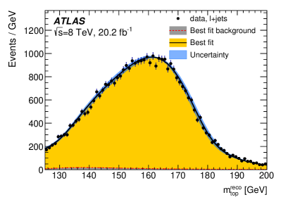
(a) Reconstructed top quark mass

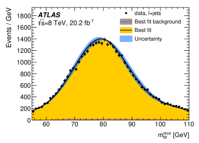
(b) Reconstructed $W$ boson mass

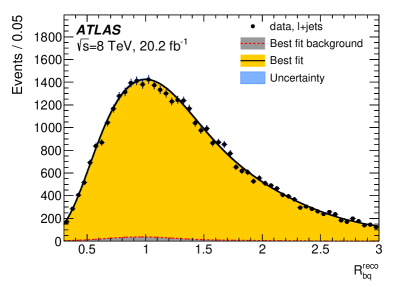
(c) Reconstructed ratio of jet transverse momenta

Figure 6: Results of the likelihood fit to the data. The figures show the data distributions of the three observables with statistical uncertainties together with the fitted probability density function for the background alone (barely visible at the bottom of the figure) and for the sum of signal and background. The uncertainty band corresponds to the one standard deviation total uncertainty in the fit function. It is based on the total uncertainty in the three fitted parameters as explained in the text. Figure (a) shows the distribution of the reconstructed top quark mass $m_{\mathrm{top}}^{\mathrm{reco}}$, figure (b) shows the distribution of the reconstructed $W$ boson mass $m_{W}^{\mathrm{reco}}$ and figure (c) shows the reconstructed ratio of jet transverse momenta $R_{bq}^{\mathrm{reco}}$.

The uncertainty band attached to the fit to data is obtained in the following way. At each point in $m_{\mathrm{top}}^{\mathrm{reco}}$, $m_{W}^{\mathrm{reco}}$ and $R_{bq}^{\mathrm{reco}}$, the band contains 68$\%$ of all fit function values obtained by randomly varying $m_{\mathrm{top}}$, $\mathrm{JSF}$ and $\mathrm{bJSF}$ within their total uncertainties and taking into account their correlations. The waist in the uncertainty band is caused by the usage of normalized probability density functions. The band visualises the variations of the three template fit functions caused by all the uncertainties in $m_{\mathrm{top}}$ listed in Table 3. The total uncertainty in all three fitted parameters is dominated by their systematic uncertainty. Therefore, the band shown is much wider than the band that would be obtained by fitting to the distributions with statistical uncertainties only.

The measured value of $m_{\mathrm{top}}$ in the $t\bar{t}\to\mathrm{lepton+jets}$ channel at ${\sqrt{s}}=8$ TeV is

$$m_{\mathrm{top}} =172.08\,\pm\,0.39\,\mathrm{(stat)}\,\pm\,0.82\,\mathrm{(syst)}\leavevmode\nobreak\ \text{Ge\kern-1.00006ptV}$$

with a total uncertainty of $0.91$ GeV. The statistical precision of the systematic uncertainty is $0.06$ GeV. This result corresponds to a $19\%$ improvement on the result obtained using the standard selection on the same data. Compared with the result in the $t\bar{t}\to\mathrm{lepton+jets}$ channel at ${\sqrt{s}}=7$ TeV, the improvement is $29\%$. On top of the smaller statistical uncertainty, the increased precision is mainly driven by smaller theory modelling uncertainties achieved by the $\mathrm{BDT}$ selection. The larger number of events in the ${\sqrt{s}}=8$ TeV dataset is effectively traded for lower systematic uncertainties, resulting in a significant gain in total precision. The new ATLAS result in the $t\bar{t}\to\mathrm{lepton+jets}$ channel is more precise than the result from the CDF experiment, but less precise than the CMS and D0 results, measured in the same channel, as shown in Figure 14(b) in Appendix B.

10 Combination with previous ATLAS results

This section presents the combination of the six $m_{\mathrm{top}}$ results of the ATLAS analyses in the $t\bar{t}\to\mathrm{dilepton}$, $t\bar{t}\to\mathrm{lepton+jets}$ and $t\bar{t}\to\mathrm{all\,jets}$ channels at centre-of-mass energies of ${\sqrt{s}}=7$ and $8$ TeV. The treatment of the results that are input to the combinations are described, followed by a detailed explanation of the evaluation of the estimator correlations for the various sources of systematic uncertainty. The compatibilities of the measured $m_{\mathrm{top}}$ values are investigated using a pairwise $\chi^{2}$ for all pairs of measurements and by evaluating the compatibility of selected combinations. Finally, the six results are combined, displaying the effect of individual results on the combined result.

10.1 Inputs to the combination and categorization of uncertainties

The measured values of the individual analyses and their statistical and systematic uncertainties are given in Table 4. For each result, the evaluated systematic uncertainties are shown together with their statistical uncertainties. The statistical uncertainties in the total systematic uncertainties and the total uncertainties are obtained from the propagation of uncertainties.

For the combinations to follow, the combined uncertainties for the previous results, namely $t\bar{t}\to\mathrm{dilepton}$ and $t\bar{t}\to\mathrm{lepton+jets}$ at ${\sqrt{s}}=7$ TeV from LABEL:\cite[cite]{[\@@bibref{}{TOPQ-2013-02}{}{}]}, $t\bar{t}\to\mathrm{all\,jets}$ at ${\sqrt{s}}=7$ TeV from LABEL:\cite[cite]{[\@@bibref{}{TOPQ-2013-03}{}{}]}, $t\bar{t}\to\mathrm{dilepton}$ at ${\sqrt{s}}=8$ TeV from LABEL:\cite[cite]{[\@@bibref{}{TOPQ-2016-03}{}{}]} and $t\bar{t}\to\mathrm{all\,jets}$ at ${\sqrt{s}}=8$ TeV from LABEL:\cite[cite]{[\@@bibref{}{TOPQ-2015-03}{}{}]}, were all re-evaluated. In all cases, the numbers agree to within 0.01 GeV with the original publications, which in any case is the rounding precision due to the precision of some of the inputs. On top of this, the results listed in Table 4 differ in some aspects from the original publications as explained below.

Table 4: The six measured values of $m_{\mathrm{top}}$ ($i=0,\ldots,5$) and their statistical and systematic uncertainty sources $k$, numbered as given in the first column. For the individual measurements, the systematic uncertainty in $m_{\mathrm{top}}$ and its associated statistical uncertainty are given for each source of uncertainty. The last line refers to the sum in quadrature of the statistical and systematic uncertainties. The statistical uncertainties in the total systematic uncertainties and in the total uncertainties are calculated from the propagation of uncertainties. Systematic uncertainties listed as 0 are not evaluated, while an empty cell indicates an uncertainty not applicable to the correponding measurement. Statistical uncertainties quoted as 0.00 are smaller than 0.005.

		${\sqrt{s}}=7$ TeV			${\sqrt{s}}=8$ TeV
		$m_{\mathrm{top}}^{\mathrm{dilepton}}$ [GeV]	$m_{\mathrm{top}}^{\mathrm{\ell+jets}}$ [GeV]	$m_{\mathrm{top}}^{\mathrm{all\,jets}}$ [GeV]	$m_{\mathrm{top}}^{\mathrm{dilepton}}$ [GeV]	$m_{\mathrm{top}}^{\mathrm{\ell+jets}}$ [GeV]	$m_{\mathrm{top}}^{\mathrm{all\,jets}}$ [GeV]
$k$	Results ($i=0\ldots,5$)	173.79	$172.33$	175.06	172.99	$172.08$	173.72
0	Statistics	0.54	$0.75$	1.35	0.41	$0.39$	0.55
	– Stat. comp. ($m_{\mathrm{top}}$)		$0.23$			$0.11$
	– Stat. comp. ($\mathrm{JSF}$)		$0.25$			$0.11$
	– Stat. comp. ($\mathrm{bJSF}$)		$0.67$			$0.35$
1	Method	0.09 $\pm$ 0.07	0.11 $\pm$ 0.10	0.42 $\pm$ 0.01	0.05 $\pm$ 0.07	0.13 $\pm$ 0.11	0.11
2	Signal Monte Carlo generator	0.26 $\pm$ 0.16	0.22 $\pm$ 0.21	0.30 $\pm$ 0.30	0.09 $\pm$ 0.15	0.16 $\pm$ 0.17	0.18 $\pm$ 0.21
3	Hadronization	0.53 $\pm$ 0.09	0.18 $\pm$ 0.12	0.50 $\pm$ 0.15	0.22 $\pm$ 0.09	0.15 $\pm$ 0.10	0.64 $\pm$ 0.15
4	Initial- and final-state QCD radiation	0.47 $\pm$ 0.05	0.32 $\pm$ 0.06	0.22 $\pm$ 0.11	0.23 $\pm$ 0.07	0.08 $\pm$ 0.11	0.10 $\pm$ 0.28
5	Underlying event	0.05 $\pm$ 0.05	0.15 $\pm$ 0.07	0.08 $\pm$ 0.10	0.10 $\pm$ 0.14	0.08 $\pm$ 0.15	0.12 $\pm$ 0.16
6	Colour reconnection	0.14 $\pm$ 0.05	0.11 $\pm$ 0.07	0.22 $\pm$ 0.10	0.03 $\pm$ 0.14	0.19 $\pm$ 0.15	0.12 $\pm$ 0.16
7	Parton distribution function	0.10 $\pm$ 0.00	0.25 $\pm$ 0.00	0.09 $\pm$ 0.00	0.05 $\pm$ 0.00	0.09 $\pm$ 0.00	0.09 $\pm$ 0.00
8	Background normalization	0.04 $\pm$ 0.00	0.10 $\pm$ 0.00		0.03 $\pm$ 0.00	0.08 $\pm$ 0.00
9	$W/Z$+jets shape	0.00 $\pm$ 0.00	0.29 $\pm$ 0.00		$0$	0.11 $\pm$ 0.00
10	Fake leptons shape	0.01 $\pm$ 0.00	0.05 $\pm$ 0.00		0.07 $\pm$ 0.00	$0$
11	Data-driven all-jets background			0.35 $\pm$ 0.21			0.17
12	Jet energy scale	0.76 $\pm$ 0.09	0.58 $\pm$ 0.11	0.50 $\pm$ 0.05	0.54 $\pm$ 0.04	0.54 $\pm$ 0.02	0.60 $\pm$ 0.03
13	Relative $b$-to-light-jet energy scale	0.68 $\pm$ 0.02	0.06 $\pm$ 0.03	0.62 $\pm$ 0.05	0.30 $\pm$ 0.01	0.03 $\pm$ 0.01	0.34 $\pm$ 0.02
14	Jet energy resolution	0.19 $\pm$ 0.04	0.22 $\pm$ 0.11	0.01 $\pm$ 0.08	0.09 $\pm$ 0.05	0.20 $\pm$ 0.04	0.10 $\pm$ 0.04
15	Jet reconstruction efficiency	0.07 $\pm$ 0.00	0.12 $\pm$ 0.00	0.01 $\pm$ 0.01	0.01 $\pm$ 0.00	0.02 $\pm$ 0.01	$0$
16	Jet vertex fraction	0.00 $\pm$ 0.00	0.01 $\pm$ 0.00	0.01 $\pm$ 0.01	0.02 $\pm$ 0.00	0.09 $\pm$ 0.01	0.03 $\pm$ 0.01
17	$b\text{-tagging}$	0.07 $\pm$ 0.00	0.50 $\pm$ 0.00	0.16 $\pm$ 0.00	0.04 $\pm$ 0.02	0.38 $\pm$ 0.00	0.10 $\pm$ 0.00
18	Leptons	0.13 $\pm$ 0.00	0.04 $\pm$ 0.00	$0$	0.14 $\pm$ 0.01	0.16 $\pm$ 0.01	0.01 $\pm$ 0.00
19	Missing transverse momentum	0.04 $\pm$ 0.03	0.15 $\pm$ 0.04	0.02 $\pm$ 0.05	0.01 $\pm$ 0.01	0.05 $\pm$ 0.01	0.01 $\pm$ 0.01
20	Pile-up	0.01 $\pm$ 0.00	0.02 $\pm$ 0.01	0.02 $\pm$ 0.00	0.05 $\pm$ 0.01	0.15 $\pm$ 0.01	0.01 $\pm$ 0.00
21	All-jets trigger			0.01 $\pm$ 0.01			0.08 $\pm$ 0.01
22	Fast vs. full simulation			0.24 $\pm$ 0.18
	Total systematic uncertainty	1.31 $\pm$ 0.07	$1.04$ $\pm$ $0.08$	1.21 $\pm$ 0.13	$0.74$ $\pm$ $0.05$	$0.82$ $\pm$ $0.06$	1.02 $\pm$ 0.11
	Total	1.42 $\pm$ 0.07	$1.28$ $\pm$ $0.08$	1.82 $\pm$ 0.13	$0.85$ $\pm$ $0.05$	$0.91$ $\pm$ $0.06$	1.16 $\pm$ 0.11

The combination follows the approach developed for the combination of ${\sqrt{s}}=7$ TeV analyses in LABEL:\cite[cite]{[\@@bibref{}{TOPQ-2013-02}{}{}]}, including the evaluation of the correlations given in Section 10.2 below. The treatment of uncertainty categories for the $t\bar{t}\to\mathrm{dilepton}$ and $t\bar{t}\to\mathrm{lepton+jets}$ measurements at ${\sqrt{s}}=7$ TeV exactly follows LABEL:\cite[cite]{[\@@bibref{}{TOPQ-2013-02}{}{}]}. The uncertainty categorizations for the $t\bar{t}\to\mathrm{all\,jets}$ measurements at ${\sqrt{s}}=7$ and $8$ TeV from Refs. [96] and [74] closely follow this categorization but have some extra, analysis-specific sources of uncertainty, as shown in Table 4. In addition, the $t\bar{t}\to\mathrm{all\,jets}$ result at ${\sqrt{s}}=8$ TeV from LABEL:\cite[cite]{[\@@bibref{}{TOPQ-2015-03}{}{}]} is based on a different treatment of the PDF-uncertainty-induced uncertainty in $m_{\mathrm{top}}$. To allow the evaluation of the estimator correlations also for this uncertainty in $m_{\mathrm{top}}$, for this combination, the respective uncertainty is newly evaluated according to the prescription given in Section 8.

For the $t\bar{t}\to\mathrm{all\,jets}$ result at ${\sqrt{s}}=7$ TeV the statistical precisions in the systematic uncertainties were not evaluated in LABEL:\cite[cite]{[\@@bibref{}{TOPQ-2013-02}{}{}]} but were calculated for this combination. For the $t\bar{t}\to\mathrm{all\,jets}$ result at ${\sqrt{s}}=8$ TeV in LABEL:\cite[cite]{[\@@bibref{}{TOPQ-2015-03}{}{}]}, for some of the sources, the statistical uncertainty in the systematic uncertainty was not evaluated, such that the quoted statistical uncertainty in the total systematic uncertainty is a lower limit.

For the mapping of uncertainty categories for data taken at different centre-of-mass energies, the choice of LABEL:\cite[cite]{[\@@bibref{}{TOPQ-2016-03}{}{}]} is employed. The most complex cases are the uncertainties involving eigenvector decompositions, such as the $\mathrm{JES}$ and $b\text{-tagging}$ scale factor uncertainties, and the uncertainty categories that do not apply to all input measurements. The JES-uncertainty-induced uncertainty in $m_{\mathrm{top}}$ is obtained from a number of $\mathrm{JES}$ subcomponents. Some $\mathrm{JES}$ subcomponents have an equivalent at the other centre-of-mass energy and others do not. As in LABEL:\cite[cite]{[\@@bibref{}{TOPQ-2016-03}{}{}]}, the $\mathrm{JES}$ subcomponents without an equivalent at the other centre-of-mass energy are treated as independent, resulting in vanishing estimator correlations for that part of the covariance matrix. For the remaining subcomponents, the estimator correlations are partly positive and partly negative. As an example, for the flavour part of the JES-uncertainty-induced uncertainty in $m_{\mathrm{top}}$, the two most precise results, the $t\bar{t}\to\mathrm{dilepton}$ and $t\bar{t}\to\mathrm{lepton+jets}$ measurements at ${\sqrt{s}}=8$ TeV, are negatively correlated. Consequently, for this pair, the resulting estimator correlation for the total JES-induced uncertainty in $m_{\mathrm{top}}$ is also negative. At the quoted precision, the two assumptions about the equivalence of the $\mathrm{JES}$ subcomponents between the datasets at the two centre-of-mass energies, i.e. the weak and strong correlation scenarios described in Table 10 in Appendix A, leave the combined value and uncertainty unchanged.

Following LABEL:\cite[cite]{[\@@bibref{}{TOPQ-2016-03}{}{}]}, the ${\sqrt{s}}=7$ and $8$ TeV measurements are treated as uncorrelated for the nuisance parameters of the $b\text{-tagging}$, $c/\tau$-tagging, mistagging and JER uncertainties. In LABEL:\cite[cite]{[\@@bibref{}{TOPQ-2016-03}{}{}]} it was shown that a correlated treatment of the flavour-tagging nuisance parameters results in an insignificant change in the combination. For the statistical, method calibration, MC-based background shape at ${\sqrt{s}}=7$ and $8$ TeV, and the pile-up uncertainties in $m_{\mathrm{top}}$, the measurements are assumed to be uncorrelated. Details of the evaluation of the correlations for all remaining systematic uncertainties are discussed below.

10.2 Mathematical framework and evaluation of estimator correlations

All combinations are performed using the best linear unbiased estimate (BLUE) method [97, 98] in a C++ implementation described in LABEL:\cite[cite]{[\@@bibref{}{BLUEcpp}{}{}]}. The BLUE method uses a linear combination of the inputs to combine measurements. The coefficients (BLUE weights) are determined via the minimization of the variance of the combined result. They can be used to construct measures for the importance of a given single measurement in the combination [98]. For any combination, the measured values $x_{i}$, the list of uncertainties $\sigma_{ik}$ and the correlations $\rho_{ijk}$ of the estimators ($i,j$) for each source of uncertainty ($k$) have to be provided. For all uncertainties, a Gaussian probability distribution function is assumed. For the uncertainties in $m_{\mathrm{top}}$ for which the measurements are correlated, when using $\pm 1\sigma$ variations of a systematic effect, e.g. when changing the $\mathrm{bJES}$ by $\pm 1\sigma$, there are two possibilities. When simultaneously applying a variation for a systematic uncertainty, e.g. $+1\sigma$ for the $\mathrm{bJES}$, to a pair ($i,j$) of measurements, e.g. the $t\bar{t}\to\mathrm{lepton+jets}$ and $t\bar{t}\to\mathrm{dilepton}$ measurements at ${\sqrt{s}}=8$ TeV, both analyses can result in a larger or smaller $m_{\mathrm{top}}$ value than the one obtained for the nominal case (full correlation, $\rho_{ijk}=+1$), or one analysis can result in a larger and the other in a smaller value (full anti-correlation, $\rho_{ijk}=-1$). Consequently, an uncertainty from a source only consisting of a single variation, such as the bJES-uncertainty-induced uncertainty or the uncertainty related to the choice of MC generator for signal events, results in a correlation of $\rho_{ijk}=\pm 1$. The estimator correlations for composite uncertainties are evaluated by calculating the correlation from the subcomponents. As an example, for the $t\bar{t}\to\mathrm{lepton+jets}$ result at ${\sqrt{s}}=8$ TeV, the subcomponents of the $\mathrm{JES}$ uncertainty are shown in Table 10 in Appendix A. For any pair of measurements ($i,j$), this evaluation is done by adding the covariance terms of the subcomponents $k$ with $\rho_{ijk}=\pm 1$ and dividing by the total uncertainties for that source. The resulting estimator correlation is

$$\rho_{ij} =\frac{\sum_{k=1}^{N_{\mathrm{comp}}}\rho_{ijk}\sigma_{ik}\sigma_{jk}}{\sigma_{i}\sigma_{j}}.$$

The quantity $\sigma^{2}_{i}=\sum_{k=1}^{N_{\mathrm{comp}}}\sigma^{2}_{ik}$ is the sum of the single subcomponent variances in analysis $i$. This procedure is applied to all uncertainty sources that consist of more than one subcomponent to reduce the large list of uncertainty subcomponents per estimator of $\mathcal{O}$(100) to a suitable number of uncertainty sources, i.e. to those given in Table 4. Since the full covariance matrix is independent of how the subsets are chosen, this does not affect the combination.

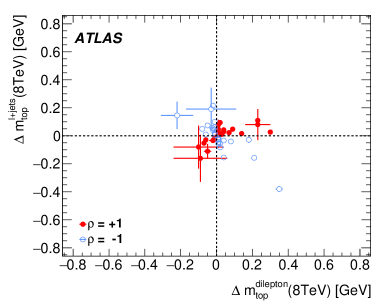
(a) $t\bar{t}\to\mathrm{dilepton}$ ($8$ TeV) and $t\bar{t}\to\mathrm{lepton+jets}$ ($8$ TeV)

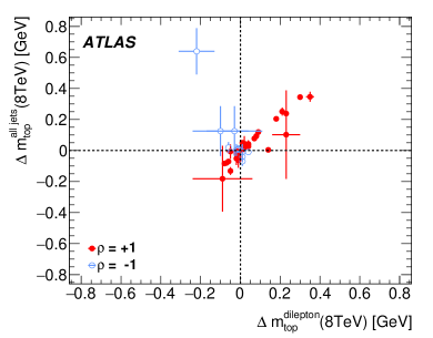
(b) $t\bar{t}\to\mathrm{dilepton}$ ($8$ TeV) and $t\bar{t}\to\mathrm{all\,jets}$ ($8$ TeV)

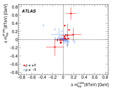
(c) $t\bar{t}\to\mathrm{lepton+jets}$ ($8$ TeV) and $t\bar{t}\to\mathrm{all\,jets}$ ($8$ TeV)

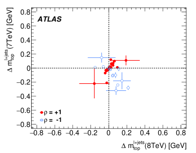
(d) $t\bar{t}\to\mathrm{lepton+jets}$ ($8$ TeV) and $t\bar{t}\to\mathrm{lepton+jets}$ ($7$ TeV)

Figure 7: The pairwise shifts in $m_{\mathrm{top}}$ when simultaneously varying a pair of measurements for a systematic uncertainty or a subcomponent of a systematic uncertainty. Figures (a) and (b) show the correlations of the $t\bar{t}\to\mathrm{dilepton}$ measurement at ${\sqrt{s}}=8$ TeV with the two other measurements at the same centre-of-mass energy for all sources of uncertainty for which the estimators are correlated. Figure (c) shows the correlations of the present measurement with the $t\bar{t}\to\mathrm{all\,jets}$ measurement at ${\sqrt{s}}=8$ TeV, while figure (d) shows the correlations of the present measurement with the $t\bar{t}\to\mathrm{lepton+jets}$ measurement at ${\sqrt{s}}=7$ TeV. The crosses indicate the statistical uncertainty in the systematic uncertainties. The solid points indicate the fully correlated cases, and the open points indicate the anti-correlated ones.

For the three analyses, the evaluated shifts in $m_{\mathrm{top}}$ per uncertainty subcomponent are referred to as $\Delta m_{\mathrm{top}}^{\mathrm{dilepton}}$, $\Delta m_{\mathrm{top}}^{\mathrm{\ell+jets}}$ and $\Delta m_{\mathrm{top}}^{\mathrm{all\,jets}}$. They are shown in Figure 7 for the various uncertainty subcomponents in selected pairs of analyses. The pairs using the results from ${\sqrt{s}}=8$ TeV data are shown in Figures 7(a)–7(c), while Figure 7(d) is for the two analyses in the $t\bar{t}\to\mathrm{lepton+jets}$ channel at the two centre-of-mass energies. Each point represents the observed shifts for a systematic uncertainty or a subcomponent of a systematic uncertainty together with a cross, indicating the corresponding statistical precision in the systematic uncertainty in the two results. The solid points indicate the fully correlated cases, and the open points indicate the anti-correlated ones.

For many significant sources of uncertainty in Figure 7(a), the $t\bar{t}\to\mathrm{lepton+jets}$ and $t\bar{t}\to\mathrm{dilepton}$ measurements are anti-correlated. As shown in LABEL:\cite[cite]{[\@@bibref{}{TOPQ-2013-02}{}{}]}, this is caused by the in situ determination of the $\mathrm{JSF}$ and $\mathrm{bJSF}$ in the three-dimensional $t\bar{t}\to\mathrm{lepton+jets}$ analysis. In contrast, for most sources of uncertainty, a positive estimator correlation is observed for the $t\bar{t}\to\mathrm{dilepton}$ and $t\bar{t}\to\mathrm{all\,jets}$ measurements at ${\sqrt{s}}=8$ TeV, shown in Figure 7(b). The prominent exception is the hadronization-uncertainty-induced uncertainty in $m_{\mathrm{top}}$, i.e. the single largest uncertainty in the $t\bar{t}\to\mathrm{all\,jets}$ measurement at ${\sqrt{s}}=8$ TeV, for which the two measurements are anti-correlated. On the contrary, the $t\bar{t}\to\mathrm{lepton+jets}$ and $t\bar{t}\to\mathrm{all\,jets}$ measurements at ${\sqrt{s}}=8$ TeV, shown in Figure 7(c), are positively correlated for this uncertainty. Finally, the $t\bar{t}\to\mathrm{lepton+jets}$ measurements at the two centre-of-mass energies in Figure 7(d) show a rather low correlation. The correlations per source of uncertainty and the total estimator correlations are summarized in Table 5.

Table 5: The pairwise correlations $\rho_{ijk}$ of the six measurements $i,j=0,\ldots,5$ of $m_{\mathrm{top}}$ for each source of systematic uncertainty $k=0,\ldots,22$, along with the total estimator correlations and the compatibility of the measurements using $\chi^{2}_{ij}$ from Eq. (2). The indices $i$ and $j$ are 0 for $t\bar{t}\to\mathrm{dilepton}$ at ${\sqrt{s}}=7$ TeV, 1 for $t\bar{t}\to\mathrm{lepton+jets}$ at ${\sqrt{s}}=7$ TeV, 2 for $t\bar{t}\to\mathrm{all\,jets}$ at ${\sqrt{s}}=7$ TeV, 3 for $t\bar{t}\to\mathrm{dilepton}$ at ${\sqrt{s}}=8$ TeV, 4 for $t\bar{t}\to\mathrm{lepton+jets}$ at ${\sqrt{s}}=8$ TeV, and 5 for $t\bar{t}\to\mathrm{all\,jets}$ at ${\sqrt{s}}=8$ TeV. The correspondence of the indices $k=0,\ldots,22$ and the sources of systematic uncertainty are given in Table 4. Correlations that are assigned, or cannot be evaluated because one uncertainty in the covariance term is zero at the quoted precision, are given as integer values, while evaluated correlations are shown as real values.

	$m_{\mathrm{top}}^{\mathrm{dilepton}}$ 7 TeV					$m_{\mathrm{top}}^{\mathrm{\ell+jets}}$ 7 TeV				$m_{\mathrm{top}}^{\mathrm{all\,jets}}$ 7 TeV			$m_{\mathrm{top}}^{\mathrm{dilepton}}$ 8 TeV		$m_{\mathrm{top}}^{\mathrm{\ell+jets}}$ 8 TeV
	$i=0$					$i=1$				$i=2$			$i=3$		$i=4$
$k$	$\rho_{01}$	$\rho_{02}$	$\rho_{03}$	$\rho_{04}$	$\rho_{05}$	$\rho_{12}$	$\rho_{13}$	$\rho_{14}$	$\rho_{15}$	$\rho_{23}$	$\rho_{24}$	$\rho_{25}$	$\rho_{34}$	$\rho_{35}$	$\rho_{45}$
0	$0$	$0$	$0$	$0$	$0$	$0$	$0$	$0$	$0$	$0$	$0$	$0$	$0$	$0$	$0$
1	$0$	$0$	$0$	$0$	$0$	$0$	$0$	$0$	$0$	$0$	$0$	$0$	$0$	$0$	$0$
2	$1.00$	$-1.00$	$1.00$	$1.00$	$1.00$	$-1.00$	$1.00$	$1.00$	$1.00$	$-1.00$	$-1.00$	$-1.00$	$1.00$	$1.00$	$1.00$
3	$1.00$	$1.00$	$1.00$	$-1.00$	$-1.00$	$1.00$	$1.00$	$-1.00$	$-1.00$	$1.00$	$-1.00$	$-1.00$	$-1.00$	$-1.00$	$1.00$
4	$-1.00$	$1.00$	$1.00$	$1.00$	$1.00$	$-1.00$	$-1.00$	$-1.00$	$-1.00$	$1.00$	$1.00$	$1.00$	$1.00$	$1.00$	$1.00$
5	$-1.00$	$1.00$	$1.00$	$1.00$	$-1.00$	$-1.00$	$-1.00$	$-1.00$	$1.00$	$1.00$	$1.00$	$-1.00$	$1.00$	$-1.00$	$-1.00$
6	$-1.00$	$1.00$	$1.00$	$-1.00$	$-1.00$	$-1.00$	$-1.00$	$1.00$	$1.00$	$1.00$	$-1.00$	$-1.00$	$-1.00$	$-1.00$	$1.00$
7	$0.53$	$0.22$	$-0.02$	$0.72$	$-0.61$	$-0.36$	$-0.32$	$0.72$	$-0.81$	$0.41$	$-0.05$	$0.27$	$-0.48$	$0.40$	$-0.76$
8	$1.00$	$0$	$0.31$	$-0.77$	$0$	$0$	$0.31$	$-0.74$	$0$	$0$	$0$	$0$	$-0.06$	$0$	$0$
9	$0$	$0$	$0$	$0$	$0$	$0$	$0$	$0$	$0$	$0$	$0$	$0$	$0$	$0$	$0$
10	$0.20$	$0$	$0$	$0$	$0$	$0$	$0.27$	$0$	$0$	$0$	$0$	$0$	$0$	$0$	$0$
11	$0$	$0$	$0$	$0$	$0$	$0$	$0$	$0$	$0$	$0$	$0$	$1$	$0$	$0$	$0$
12	$-0.24$	$0.86$	$0.36$	$0.18$	$0.36$	$0.10$	$0.04$	$-0.29$	$0.13$	$0.41$	$0.09$	$0.42$	$-0.54$	$0.98$	$-0.57$
13	$1.00$	$1.00$	$1.00$	$1.00$	$1.00$	$1.00$	$1.00$	$1.00$	$1.00$	$1.00$	$1.00$	$1.00$	$1.00$	$1.00$	$1.00$
14	$-1.00$	$1.00$	$0$	$0$	$0$	$-1.00$	$0$	$0$	$0$	$0$	$0$	$0$	$0.22$	$-0.07$	$-0.17$
15	$1.00$	$1.00$	$1.00$	$1.00$	$0$	$1.00$	$1.00$	$1.00$	$0$	$1.00$	$1.00$	$0$	$1.00$	$0$	$0$
16	$-1.00$	$1.00$	$-1.00$	$-1.00$	$-1.00$	$-1.00$	$1.00$	$1.00$	$1.00$	$-1.00$	$-1.00$	$-1.00$	$1.00$	$1.00$	$1.00$
17	$-0.80$	$-0.03$	$0$	$0$	$0$	$0$	$0$	$0$	$0$	$0$	$0$	$0$	$-0.23$	$1$	$1$
18	$-0.35$	$0$	$0.93$	$-0.08$	$0.42$	$0$	$-0.51$	$-0.17$	$0.02$	$0$	$0$	$0$	$0.11$	$0.28$	$-0.36$
19	$0.00$	$-0.26$	$-0.26$	$-0.12$	$0.04$	$0.84$	$0.26$	$0.22$	$0.16$	$0$	$0$	$0$	$0.97$	$0.86$	$0.96$
20	$0$	$0$	$0$	$0$	$0$	$0$	$0$	$0$	$0$	$0$	$0$	$0$	$0$	$0$	$0$
21	$0$	$0$	$0$	$0$	$0$	$0$	$0$	$0$	$0$	$0$	$0$	$1.00$	$0$	$0$	$0$
22	$0$	$0$	$0$	$0$	$0$	$0$	$0$	$0$	$0$	$0$	$0$	$0$	$0$	$0$	$0$
Total	$-0.07$	$0.42$	$0.52$	$0.06$	$0.08$	$-0.01$	$-0.00$	$-0.07$	$-0.02$	$0.29$	$-0.06$	$-0.01$	$-0.19$	$0.32$	$0.00$
$\chi^{2}_{ij}$	$0.55$	$0.51$	$0.44$	$1.09$	$0.00$	$1.50$	$0.18$	$0.02$	$0.64$	$1.37$	$2.06$	$0.39$	$0.45$	$0.37$	$1.25$

The improvement in the combination obtained by the use of evaluated correlations compared with using estimator correlations assigned solely by physics assessments (here referred to as assigned correlations) is quantified using an example. Using the choices of assigned correlations from LABEL:\cite[cite]{[\@@bibref{}{ATLAS:2014wva}{}{}]} for the ATLAS results in the $t\bar{t}\to\mathrm{dilepton}$ and $t\bar{t}\to\mathrm{lepton+jets}$ channels at ${\sqrt{s}}=7$ TeV listed in Table 4 gives a combined value of $m_{\mathrm{top}}=172.91\,\pm\,0.50\,\mathrm{(stat)}\,\pm\,1.05\,\mathrm{(syst)}$ GeV compared with $m_{\mathrm{top}}=172.99\,\pm\,0.48\,\mathrm{(stat)}\,\pm\,0.78\,\mathrm{(syst)}$ GeV. The significant improvement in the precision of the combination demonstrates the particular importance of evaluating the correlations.

For the combinations presented in this paper, most estimator correlations could be evaluated. The most prominent exception is for the $b\text{-tagging}$ uncertainty, where the $t\bar{t}\to\mathrm{all\,jets}$ measurement at ${\sqrt{s}}=8$ TeV is based on a different $b\text{-tagging}$ algorithm and calibration than the $t\bar{t}\to\mathrm{dilepton}$ and $t\bar{t}\to\mathrm{lepton+jets}$ measurements at ${\sqrt{s}}=8$ TeV. It was verified that assignments of the estimator correlations of $\rho_{i5k}\in[-1,1]$, with $i=3,4$ and $k=17$, yield insignificant differences in the full combination. Estimator correlations of $\rho_{i5}=1$ are assigned for this case, as this choice gives the largest uncertainty in the combination. A similar situation arises for the data-driven all-jets background uncertainty in the two $t\bar{t}\to\mathrm{all\,jets}$ measurements, where the method used for the background estimate is similar but not identical for the two measurements. Consequently, the conservative ad hoc assignment of $\rho_{25k}=1$ was also made for this source $k=11$.

10.3 Compatibility of the inputs and selected combinations

Before any combination is performed, the compatibility of the input results is verified. For each pair of results, their compatibility is expressed by the ratio of the squared difference between the pair of measured values and the uncertainty in this difference [98] as

$$\chi^{2}_{ij} =\frac{(x_{i}-x_{j})^{2}}{\sigma_{i}^{2}+\sigma_{j}^{2}-2\rho_{ij}\sigma_{i}\sigma_{j}}.$$ (2)

The corresponding values are given in Table 5. Analysing the $\chi^{2}_{ij}$ values reveals good $\chi^{2}$ probabilities, with the smallest $\chi^{2}$ probability being $P(\chi^{2},1)=15\%$. The largest sum of $\chi^{2}_{ij}$ values by far is observed for the $t\bar{t}\to\mathrm{all\,jets}$ result at ${\sqrt{s}}=7$ TeV.

The dependences of the combined values and their uncertainties on the total correlation for pairwise combinations of results are analysed. The dependences for pairs of the three results from ${\sqrt{s}}=8$ TeV data are shown in Figure 8. The largest information gain is achieved by combining the $t\bar{t}\to\mathrm{dilepton}$ and $t\bar{t}\to\mathrm{lepton+jets}$ results at ${\sqrt{s}}=8$ TeV, shown in Figures 8(a) and 8(b), which are anti-correlated, i.e. $\rho=-0.19$.

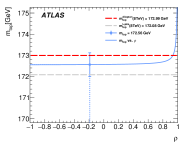
(a) $t\bar{t}\to\mathrm{dilepton}$ ($8$ TeV) and $t\bar{t}\to\mathrm{lepton+jets}$ ($8$ TeV)

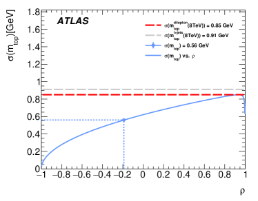
(b) $t\bar{t}\to\mathrm{dilepton}$ ($8$ TeV) and $t\bar{t}\to\mathrm{lepton+jets}$ ($8$ TeV)

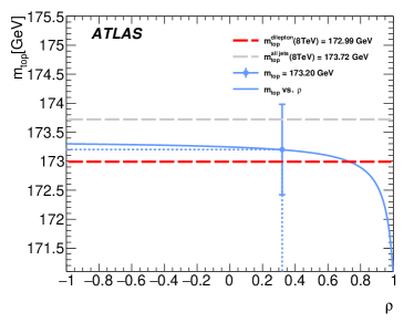
(c) $t\bar{t}\to\mathrm{dilepton}$ ($8$ TeV) and $t\bar{t}\to\mathrm{all\,jets}$ ($8$ TeV)

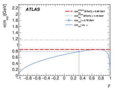
(d) $t\bar{t}\to\mathrm{dilepton}$ ($8$ TeV) and $t\bar{t}\to\mathrm{all\,jets}$ ($8$ TeV)

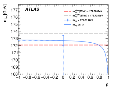
(e) $t\bar{t}\to\mathrm{lepton+jets}$ ($8$ TeV) and $t\bar{t}\to\mathrm{all\,jets}$ ($8$ TeV)

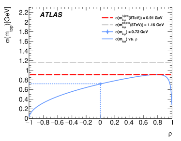
(f) $t\bar{t}\to\mathrm{lepton+jets}$ ($8$ TeV) and $t\bar{t}\to\mathrm{all\,jets}$ ($8$ TeV)

Figure 8: The combined values (left) and uncertainties (right) of the combination of pairs of individual results at ${\sqrt{s}}=8$ TeV, shown as functions of the total correlation $\rho$ (solid lines). The combination of the $t\bar{t}\to\mathrm{dilepton}$ and $t\bar{t}\to\mathrm{lepton+jets}$ results is shown in the top row. The middle row is for the combination of the $t\bar{t}\to\mathrm{dilepton}$ and $t\bar{t}\to\mathrm{all\,jets}$ results. Finally, the combination of the $t\bar{t}\to\mathrm{lepton+jets}$ and $t\bar{t}\to\mathrm{all\,jets}$ results is shown in the bottom row. For comparison, the corresponding values for the input results are also shown (dashed lines).

Based on Tables 4 and 5, selected combinations are analysed, yielding the results given in Table 6 and shown in Figure 9. The BLUE weights and the pulls of the results are given in Table 7.

Table 6: The results for selected combinations based on the six results at ${\sqrt{s}}=7$ and $8$ TeV. The left two columns of results show the combination of the three results at ${\sqrt{s}}=7$ TeV ($m_{\mathrm{top}}^{\mathrm{7TeV}}$) or at ${\sqrt{s}}=8$ TeV ($m_{\mathrm{top}}^{\mathrm{8TeV}}$), both combinations neglecting the results at the respective other centre-of-mass energy. The middle three columns show the combination of the six results as if pairs of measurements would determine a decay-specific top quark mass, namely $m_{\mathrm{top}}^{\mathrm{dilepton}}$, $m_{\mathrm{top}}^{\mathrm{\ell+jets}}$ and $m_{\mathrm{top}}^{\mathrm{all\,jets}}$. Finally, shown on the right is the combination of the three most important results in the combination denoted by $m_{\mathrm{top}}^{\mathrm{(3)}}$ and the combination of all results, i.e. the ATLAS result for $m_{\mathrm{top}}$ shown in Figure 10. For each combination, the uncertainty is given for each source of uncertainty. Uncertainties quoted as 0.00 are smaller than 0.005, while empty cells indicate uncertainties that do not apply to the respective combination. Finally, the total systematic uncertainty and the sum in quadrature of the statistical and systematic uncertainties are given. Both are quoted including the precision at which the respective uncertainty is known.

	$m_{\mathrm{top}}^{\mathrm{7TeV}}$ [GeV]	$m_{\mathrm{top}}^{\mathrm{8TeV}}$ [GeV]	$m_{\mathrm{top}}^{\mathrm{dilepton}}$ [GeV]	$m_{\mathrm{top}}^{\mathrm{\ell+jets}}$ [GeV]	$m_{\mathrm{top}}^{\mathrm{all\,jets}}$ [GeV]	$m_{\mathrm{top}}^{\mathrm{(3)}}$ [GeV]	$m_{\mathrm{top}}$ [GeV]
Results	$173.20$	$172.68$	172.98	172.13	174.08	$172.51$	$172.69$
Statistics	$0.46$	$0.26$	0.39	0.37	0.56	$0.27$	$0.25$
Method	0.08	0.06	0.05	0.10	0.14	0.06	0.06
Signal Monte Carlo generator	0.17	0.13	0.12	0.15	0.03	0.14	0.12
Hadronization	0.35	0.04	0.18	0.03	0.32	0.07	0.00
Initial- and final-state QCD radiation	0.03	0.15	0.26	0.07	0.13	0.07	0.07
Underlying event	0.05	0.07	0.10	0.01	0.06	0.05	0.03
Colour reconnection	0.02	0.08	0.02	0.16	0.02	0.08	0.08
Parton distribution function	0.15	0.03	0.05	0.13	0.08	0.07	0.05
Background normalization	0.07	0.04	0.03	0.04	0.00	0.03	0.02
$W/Z$+jets shape	0.15	0.05	0.01	0.12	0.00	0.07	0.06
Fake leptons shape	0.03	0.03	0.07	0.02	0.00	0.03	0.03
Data-driven all-jets background	0.04	0.02	0.01	0.01	0.22		0.03
Jet energy scale	0.40	0.27	0.53	0.34	0.51	0.21	0.22
Relative $b$-to-light-jet energy scale	0.35	0.19	0.32	0.01	0.41	0.15	0.17
Jet energy resolution	0.04	0.10	0.09	0.16	0.07	0.10	0.09
Jet reconstruction efficiency	0.09	0.01	0.01	0.05	0.00	0.03	0.03
Jet vertex fraction	0.00	0.05	0.02	0.07	0.02	0.05	0.05
$b\text{-tagging}$	0.24	0.18	0.05	0.30	0.09	0.17	0.17
Leptons	0.04	0.10	0.14	0.11	0.01	0.09	0.08
Missing transverse momentum	0.08	0.03	0.01	0.07	0.01	0.04	0.04
Pile-up	0.01	0.07	0.05	0.10	0.01	0.06	0.06
All-jets trigger	0.00	0.01	0.00	0.00	0.06		0.01
Fast vs. full simulation	0.03		0.01	0.01	0.07		0.01
Total systematic uncertainty	$0.76$ $\pm$ 0.04	$0.48$ $\pm$ 0.04	0.74 $\pm$ 0.04	0.61 $\pm$ 0.04	0.80 $\pm$ 0.05	$0.42$ $\pm$ $0.04$	$0.41$ $\pm$ $0.03$
Total	$0.89$ $\pm$ 0.04	$0.54$ $\pm$ 0.04	0.84 $\pm$ 0.04	0.71 $\pm$ 0.04	0.98 $\pm$ 0.05	$0.50$ $\pm$ $0.04$	$0.48$ $\pm$ $0.03$

Table 7: The BLUE weights and the pulls of the results for the combinations reported in Table 6. The upper part refers to the independent combinations of the three results per centre-of-mass energy resulting in uncorrelated results $m_{\mathrm{top}}^{\mathrm{7TeV}}$ and $m_{\mathrm{top}}^{\mathrm{8TeV}}$. The middle part is for the combination of the three observables from pairs of results per $t\bar{t}$ decay channel, resulting in correlated results $m_{\mathrm{top}}^{\mathrm{dilepton}}$, $m_{\mathrm{top}}^{\mathrm{\ell+jets}}$ and $m_{\mathrm{top}}^{\mathrm{all\,jets}}$. The lower part refers to the combination of the three most important results $m_{\mathrm{top}}^{\mathrm{(3)}}$ and of all results $m_{\mathrm{top}}$.

		${\sqrt{s}}=7$ TeV			${\sqrt{s}}=8$ TeV
		$m_{\mathrm{top}}^{\mathrm{dilepton}}$	$m_{\mathrm{top}}^{\mathrm{\ell+jets}}$	$m_{\mathrm{top}}^{\mathrm{all\,jets}}$	$m_{\mathrm{top}}^{\mathrm{dilepton}}$	$m_{\mathrm{top}}^{\mathrm{\ell+jets}}$	$m_{\mathrm{top}}^{\mathrm{all\,jets}}$
$m_{\mathrm{top}}^{\mathrm{7TeV}}$	weight	$0.36$	$0.51$	$0.13$
	pull	$0.54$	$-0.95$	$1.18$
$m_{\mathrm{top}}^{\mathrm{8TeV}}$	weight				$0.45$	$0.44$	$0.12$
	pull				$0.48$	$-0.82$	$1.02$
$m_{\mathrm{top}}^{\mathrm{dilepton}}$	weight	$0.08$	$-0.04$	$-0.04$	$0.92$	$0.04$	$0.04$
$m_{\mathrm{top}}^{\mathrm{\ell+jets}}$	weight	$-0.09$	$0.33$	$0.03$	$0.09$	$0.67$	$-0.03$
$m_{\mathrm{top}}^{\mathrm{all\,jets}}$	weight	$-0.04$	$-0.01$	$0.30$	$0.04$	$0.01$	$0.71$
	pull	$0.71$	$0.18$	$0.64$	$0.05$	$-0.09$	$-0.58$
$m_{\mathrm{top}}^{\mathrm{(3)}}$	weight		$0.17$		$0.43$	$0.40$
	pull		$-0.16$		$0.70$	$-0.57$
$m_{\mathrm{top}}$	weight	$-0.03$	$0.16$	$0.04$	$0.35$	$0.37$	$0.10$
	pull	$0.83$	$-0.30$	$1.36$	$0.43$	$-0.79$	$0.98$

To investigate the difference in precision of combined results obtained from ${\sqrt{s}}=7$ and $8$ TeV results, two independent combinations of the three results per centre-of-mass energy are performed. For each decay channel, the results at ${\sqrt{s}}=8$ TeV are significantly more precise than those at ${\sqrt{s}}=7$ TeV. In addition, the two most precise results per centre-of-mass energy are significantly less correlated at ${\sqrt{s}}=8$ TeV than at ${\sqrt{s}}=7$ TeV. Consequently, the size of the uncertainty of the combined result at ${\sqrt{s}}=8$ TeV ($m_{\mathrm{top}}^{\mathrm{8TeV}}$) is $39\%$ smaller than the one obtained from the results at ${\sqrt{s}}=7$ TeV ($m_{\mathrm{top}}^{\mathrm{7TeV}}$). As shown in Figures 13(a) and 13(b) in Appendix B, for both centre-of-mass energies, the combination is dominated by the results in the $t\bar{t}\to\mathrm{dilepton}$ and $t\bar{t}\to\mathrm{lepton+jets}$ channels.

To investigate whether the measured $m_{\mathrm{top}}$ depends on the $t\bar{t}$ decay mode, a combination of the six results is performed in which the results in the three $t\bar{t}$ decay channels are treated as determining potentially different masses, namely $m_{\mathrm{top}}^{\mathrm{dilepton}}$, $m_{\mathrm{top}}^{\mathrm{\ell+jets}}$ and $m_{\mathrm{top}}^{\mathrm{all\,jets}}$. In such a combination, results obtained in one decay channel influence the combined result in another decay channel by means of their estimator correlation. Therefore, for each observable, e.g. $m_{\mathrm{top}}^{\mathrm{dilepton}}$, by construction the sum of weights of the results in the corresponding decay channel equals unity, while for each of the other decay channels the sum of weights of the results equals zero [100]. The combination yields compatible results for the three masses listed in Table 6. Consequently, the data do not show any sign of a decay-channel-dependent $m_{\mathrm{top}}$. The correlation matrix of the three observables 0, 1 and 2 corresponding to $m_{\mathrm{top}}^{\mathrm{dilepton}}$, $m_{\mathrm{top}}^{\mathrm{\ell+jets}}$ and $m_{\mathrm{top}}^{\mathrm{all\,jets}}$ is

$$\rho_{m_{\mathrm{top}}} =\left(\begin{array}[]{rrr}1&-0.14&0.43\\ -0.14&1&-0.05\\ 0.43&-0.05&1\end{array}\right),$$ (6)

and the smallest $\chi^{2}$ probability of any pair of combined results for determining the same $m_{\mathrm{top}}$ is $P(\chi^{2},1)=11\%$. As shown in Figures 13(c)–13(e) in Appendix B, for the combination of the three observables, the results based on ${\sqrt{s}}=7$ TeV data lead to significant improvements on their more precise counterparts obtained from ${\sqrt{s}}=8$ TeV data, apart from the $t\bar{t}\to\mathrm{dilepton}$ channel.

Given that no dependence of $m_{\mathrm{top}}$ on the centre-of-mass energy or the $t\bar{t}$ decay channel is expected, the above examples of combinations are merely additional investigations of the compatibility of the input results. The compatibility combinations are summarized in Figure 9 and listed in Table 6. For all combinations, the values quoted in Figure 9 are the combined value, the statistical uncertainty, the systematic uncertainty, the total uncertainty and the statistical uncertainty in the total uncertainty.

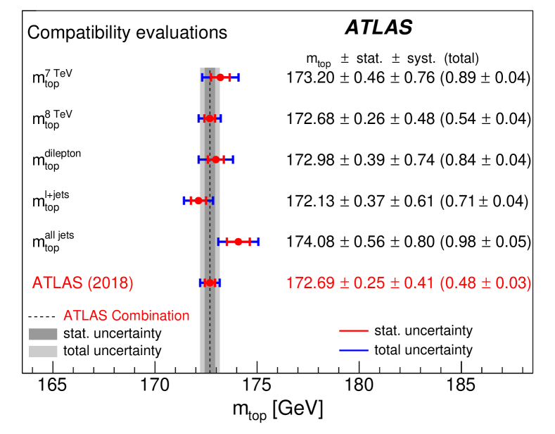
Figure 9: The compatibility combinations performed for the six ATLAS results of $m_{\mathrm{top}}$. The figure shows the combined results listed in Table 6, which are obtained from data taken at different centre-of-mass energies and for the three decay channels, in comparison to the new ATLAS result. The values quoted are the combined value, the statistical uncertainty, the systematic uncertainty, the total uncertainty and the uncertainty in the total uncertainty. The results are compared with the new ATLAS combination listed in the last line and shown as the grey vertical bands.

10.4 The combined result of $m_{\mathrm{top}}$

The use of the statistical uncertainties in the systematic uncertainties has two main advantages. Firstly, it allows a determination of the uncertainties in the evaluation of the total correlations of the estimators, avoiding the need to perform ad hoc variations. Secondly, it enables the monitoring of the evolution of the combined result in relation to the precision in its uncertainty while including results, thereby evaluating their influence on the combination. The significance of the individual results in the combination is shown in Figure 10. The individual results are shown in Figure 10(a). Their combination is displayed in Figure 10(b) where, following LABEL:\cite[cite]{[\@@bibref{}{BLUERN}{}{}]}, starting from the most precise result, i.e. the $t\bar{t}\to\mathrm{dilepton}$ measurement at ${\sqrt{s}}=8$ TeV, results are added to the combination one at a time according to their importance, and the combined result is reported.

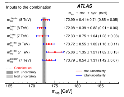
(a) Inputs to the combination

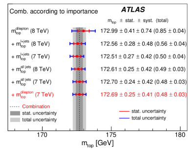
(b) Combination according to importance

Figure 10: The combination of the six ATLAS results of $m_{\mathrm{top}}$ according to importance LABEL:\cite[cite]{[\@@bibref{}{BLUERN}{}{}]}. Figure (a) shows the inputs to the combination. Figure (b) shows results of the combination when successively adding results to the most precise one. The values quoted are the combined value, the statistical uncertainty, the systematic uncertainty, the total uncertainty and the uncertainty in the total uncertainty. In this figure, each line shows the combined result when adding the result listed to the combination indicated by a ‘+’. The new ATLAS combination is given in the last line, and shown in both figures as the vertical grey bands.

Each following line of this figure shows the combined result when adding the result listed to the input of the combination, indicated by the ‘+’ in front of the name of the added estimate. The last line in Figure 10(b) shows the new ATLAS combined value of $m_{\mathrm{top}}$.

The inclusion of the $t\bar{t}\to\mathrm{lepton+jets}$ result at ${\sqrt{s}}=8$ TeV leads to the result quoted in the second line, which improves the combined uncertainty by much more than the statistical precision in the uncertainty of the most precise result. The same is found when adding the $t\bar{t}\to\mathrm{lepton+jets}$ result at ${\sqrt{s}}=7$ TeV and comparing with the statistical uncertainty in the previous combination, albeit at a much reduced significance. The corresponding result obtained from these three results, denoted by $m_{\mathrm{top}}^{\mathrm{(3)}}$, is also listed in Table 6.

The improvement in the combination by applying the $\mathrm{BDT}$ selection to the $t\bar{t}\to\mathrm{lepton+jets}$ analysis at ${\sqrt{s}}=8$ TeV is sizeable. This is seen from repeating the combination of $m_{\mathrm{top}}^{\mathrm{(3)}}$ but using the result from the standard selection from Table 3. With this, the correlation of the ${\sqrt{s}}=8$ TeV $t\bar{t}\to\mathrm{lepton+jets}$ result with the ${\sqrt{s}}=8$ TeV $t\bar{t}\to\mathrm{dilepton}$ result changes from $-0.19$ to $-0.02$. The resulting uncertainty in the combination is $0.59\,\pm\,0.05$ GeV, i.e. the combination is $18\%$ less precise than $m_{\mathrm{top}}^{\mathrm{(3)}}$ obtained using the result from the $\mathrm{BDT}$ selection. Adding the remaining results reduces the quoted combined uncertainty by $0.02$ GeV, which is smaller than the statistical precision in the uncertainty of the previously achieved result of $m_{\mathrm{top}}^{\mathrm{(3)}}$.

The changes in statistical uncertainties in the combined value and its uncertainty due to variations of the input systematic uncertainties within their uncertainties are evaluated for two cases, namely for $m_{\mathrm{top}}^{\mathrm{(3)}}$ and for the combination of all results. Following LABEL:\cite[cite]{[\@@bibref{}{TOPQ-2016-03}{}{}]}, the distributions of the combined values and uncertainties are calculated from 500 combinations, where for each combination, the sizes of the uncertainties as well as the correlations are newly evaluated. Due to the re-evaluation of the correlation, the resulting distributions are not Gaussian and are also not exactly centred around the combined value and the combined uncertainty. For $m_{\mathrm{top}}^{\mathrm{(3)}}$, the root mean square of the distribution of the combined value is $0.03$ GeV, and that of the distribution of its uncertainty is $0.04$ GeV. The corresponding values for the new ATLAS combination are $0.07$ GeV and $0.03$ GeV, respectively.

The full breakdown of uncertainties for the new combined ATLAS result for $m_{\mathrm{top}}$ is reported in the last column of Table 6. The combined result is

$$m_{\mathrm{top}} =172.69\,\pm\,0.25\,\mathrm{(stat)}\,\pm\,0.41\,\mathrm{(syst)}\leavevmode\nobreak\ \text{Ge\kern-1.00006ptV}$$

with a total uncertainty of $0.48\pm 0.03$ GeV, where the quoted uncertainty in this uncertainty is statistical. This means that the uncertainty in this combined result is only known to this precision, which, given its size, is fully adequate.

The $\chi^{2}$ probability of $m_{\mathrm{top}}^{\mathrm{(3)}}$ is $78\%$. Driven by the larger pulls of the remaining three results listed in Table 7, the $\chi^{2}$ probability of $64\%$ for the new ATLAS combination of $m_{\mathrm{top}}$ is lower but still good. The new ATLAS combined result of $m_{\mathrm{top}}$ provides a $44\%$ improvement relative to the most precise single input result, which is the $t\bar{t}\to\mathrm{dilepton}$ analysis at ${\sqrt{s}}=8$ TeV. With a relative precision of $0.28\%$, it improves on the previous combination in LABEL:\cite[cite]{[\@@bibref{}{TOPQ-2016-03}{}{}]} by $31\%$ and supersedes it. As shown in Appendix B, the new ATLAS combined result of $m_{\mathrm{top}}$ is more precise than the results from the CDF and D0 experiments, and has a precision similar to the CMS combined result.

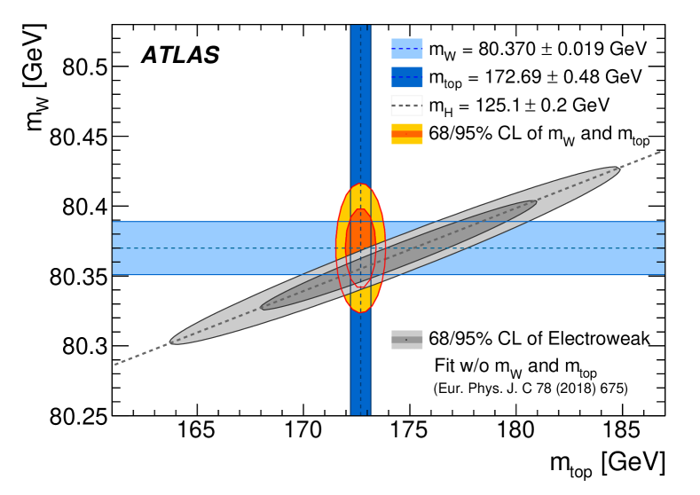
Figure 11: Comparison of indirect determinations and direct measurements of the top quark and $W$ boson masses. The direct ATLAS measurements of $m_{W}$ and $m_{\mathrm{top}}$ are shown as the horizontal and vertical bands, respectively. Their 68$\%$ and 95$\%$ confidence-level (CL) contours are compared with the corresponding results from the electroweak fit.

In Figure 11, the 68$\%$ and 95$\%$ confidence-level contours of the indirect determination of $m_{W}$ and $m_{\mathrm{top}}$ from the global electroweak fit in LABEL:\cite[cite]{[\@@bibref{}{Baak2014}{}{}]} are compared with the corresponding confidence-level contours of the direct ATLAS measurements of the two masses. The top quark mass used in this figure was obtained above, while the $W$ boson mass is taken from LABEL:\cite[cite]{[\@@bibref{}{STDM-2014-18}{}{}]}. The electroweak fit uses as input the LHC combined result of the Higgs boson mass of $m_{H}=125.09\pm 0.24$ GeV from LABEL:\cite[cite]{[\@@bibref{}{HIGG-2014-14}{}{}]}. There is good agreement between the direct ATLAS mass measurements and their indirect determinations by the electroweak fit.

11 Conclusion

The top quark mass is measured via a three-dimensional template method in the $t\bar{t}\to\mathrm{lepton+jets}$ channel and combined with previous ATLAS $m_{\mathrm{top}}$ measurements at the LHC.

For the $t\bar{t}\to\mathrm{lepton+jets}$ analysis from ${\sqrt{s}}=8$ TeV proton–proton collision data with an integrated luminosity of about $20.2$ $\mathrm{fb}^{-1}$, the event selection of the corresponding ${\sqrt{s}}=7$ TeV analysis is refined. An optimization employing a $\mathrm{BDT}$ selection to efficiently suppress less-well-reconstructed events results in a significant reduction in total uncertainty, driven by a significant decrease in theory-modelling-induced uncertainties. With this approach, the measured value of $m_{\mathrm{top}}$ is

$$m_{\mathrm{top}} =172.08\,\pm\,0.39\,\mathrm{(stat)}\,\pm\,0.82\,\mathrm{(syst)}\leavevmode\nobreak\ \text{Ge\kern-1.00006ptV}$$

with a total uncertainty of $0.91\pm 0.06$ GeV, where the quoted uncertainty in the total uncertainty is statistical. The precision is limited by systematic uncertainties, mostly by uncertainties in the calibration of the jet energy scale, $b\text{-tagging}$ and the Monte Carlo modelling of signal events. This result is more precise than the result from the CDF experiment, but less precise than the CMS and D0 results, measured in the same channel.

The correlations of six measurements of $m_{\mathrm{top}}$, performed in the three $t\bar{t}$ decay channels from ${\sqrt{s}}=7$ and 8 TeV ATLAS data, are evaluated for all sources of the systematic uncertainty. Using a dedicated mapping of uncertainty categories, combinations are performed, where measurements are added one at a time according to their importance. Treating the pairs of measurements in the three $t\bar{t}$ decay channels as determining potentially different masses, namely $m_{\mathrm{top}}^{\mathrm{dilepton}}$, $m_{\mathrm{top}}^{\mathrm{\ell+jets}}$ and $m_{\mathrm{top}}^{\mathrm{all\,jets}}$, yields consistent values within uncertainties, i.e. the data do not show any sign of a decay-channel-dependent $m_{\mathrm{top}}$.

The combined result of $m_{\mathrm{top}}$ from the six measurements is

$$m_{\mathrm{top}} =172.69\,\pm\,0.25\,\mathrm{(stat)}\,\pm\,0.41\,\mathrm{(syst)}\leavevmode\nobreak\ \text{Ge\kern-1.00006ptV}$$

with a total uncertainty of $0.48\pm 0.03$ GeV, where the quoted uncertainty in the total uncertainty is statistical. This combination is dominated by three input measurements: the measurement in the $t\bar{t}\to\mathrm{dilepton}$ channel from ${\sqrt{s}}=8$ TeV data and the two measurements in the $t\bar{t}\to\mathrm{lepton+jets}$ channel from ${\sqrt{s}}=8$ and 7 TeV data. With a relative precision of $0.28\%$, this new ATLAS combination of $m_{\mathrm{top}}$ is more precise than the result from the CDF and D0 experiments and has a precision similar to the CMS combined result. This result supersedes the previous combined ATLAS result.

With this precision in $m_{\mathrm{top}}$ achieved, precise knowledge of the relation between the mass definition of the experimental analysis and the pole mass is becoming relevant. The combined result is mostly limited by the uncertainties in the calibration of the jet energy scales, $b\text{-tagging}$ and in the Monte Carlo modelling of signal events.

Appendices

Appendix A Results from the BDT optimization and individual sources of systematic uncertainty

This appendix has additional details of the measurement of $m_{\mathrm{top}}$ in the $t\bar{t}\to\mathrm{lepton+jets}$ channel from ${\sqrt{s}}=8$ TeV data discussed in the main text.

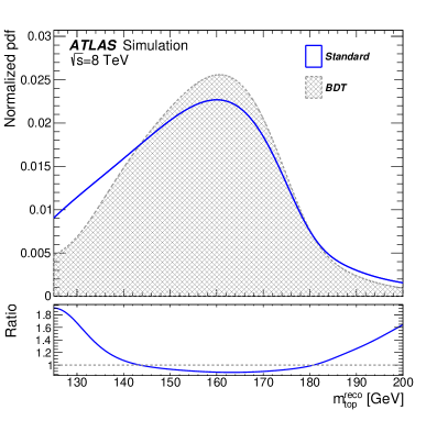
(a) Reconstructed top quark mass

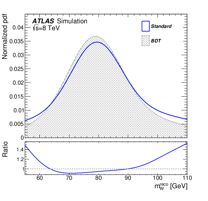
(b) Reconstructed $W$ boson mass

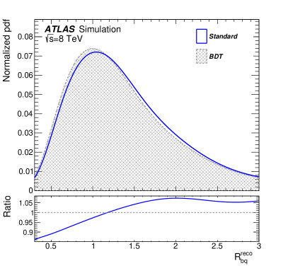
(c) Reconstructed ratio of jet transverse momenta

Figure 12: Comparison of the template fit functions of the three observables for the standard event selection (solid line) and the $\mathrm{BDT}$ event selection (dashed line). The ratios (standard / $\mathrm{BDT}$) of the pairs of functions are also shown. Figure (a) shows the reconstructed top quark mass $m_{\mathrm{top}}^{\mathrm{reco}}$, figure (b) shows the reconstructed $W$ boson mass $m_{W}^{\mathrm{reco}}$ and figure (c) shows the reconstructed jet-$p_{\text{T}}$ ratio $R_{bq}^{\mathrm{reco}}$.

In Figure 12, the template fit functions of the three observables are compared for the standard and the $\mathrm{BDT}$ event selection. The distributions of $m_{\mathrm{top}}^{\mathrm{reco}}$ and $m_{W}^{\mathrm{reco}}$ are narrower for the $\mathrm{BDT}$ event selection, which means the resolution in the two masses is improved compared with what is observed for the standard selection. The $R_{bq}^{\mathrm{reco}}$ distribution is slightly shifted to lower values for the $\mathrm{BDT}$ event selection, but the difference is small.

For the $\mathrm{BDT}$ selection, a number of systematic uncertainties listed in Table 3 are calculated by performing pseudo-experiments for more than one systematic variation. The individual components are given in Tables 8–12 below. Whenever the uncertainty is obtained from just a pair of samples, the shift $\Delta m_{\mathrm{top}}$ is listed together with the definition of the difference evaluated indicating the direction of the shift. For the other cases, the shift in $m_{\mathrm{top}}$ is quoted relative to the value measured in the central sample for the upward variation ($\Delta m_{\mathrm{top}}^{\mathrm{up}}$), the downward variation ($\Delta m_{\mathrm{top}}^{\mathrm{dw}}$) and the final shift assigned to this uncertainty component ($\Delta m_{\mathrm{top}}$). For most of the cases the signs of $\Delta m_{\mathrm{top}}^{\mathrm{up}}$ and $\Delta m_{\mathrm{top}}^{\mathrm{dw}}$ are different, indicating that $m_{\mathrm{top}}$ from the central sample is surrounded by the values from the two variations. In this case $|\Delta m_{\mathrm{top}}|$ is $0.5\cdot|\Delta m_{\mathrm{top}}^{\mathrm{up}}-\Delta m_{\mathrm{top}}^{\mathrm{dw}}|$, otherwise it is the maximum of $|\Delta m_{\mathrm{top}}^{\mathrm{up}}|$ and $|\Delta m_{\mathrm{top}}^{\mathrm{dw}}|$. In both cases, the sign of $\Delta m_{\mathrm{top}}$ is the one from $\Delta m_{\mathrm{top}}^{\mathrm{up}}$.

Table 8: The individual components of the uncertainty sources considered for the $t\bar{t}\to\mathrm{lepton+jets}$ analysis at ${\sqrt{s}}=8$ TeV for the sources of uncertainty not documented in Tables 9–12. The uncertainties together with their statistical precisions are listed in boldface and given with 0.01 GeV precision. The uncertainty per source is calculated as the sum in quadrature of the subcomponents. Uncertainties quoted as 0.00 (0.000) are smaller than 0.005 (0.0005).

Uncertainty	$\Delta m_{\mathrm{top}}^{\mathrm{up}}$ [GeV]	$\Delta m_{\mathrm{top}}^{\mathrm{dw}}$ [GeV]	$\Delta m_{\mathrm{top}}$ [GeV]
Signal Monte Carlo generator	$0.16\pm 0.17$
Powheg-Box - MC@NLO (Herwig)			$-0.161\pm 0.168$
Hadronization	$0.15\pm 0.10$
Powheg+Pythia - Powheg+Herwig			$+0.146\pm 0.098$
Initial- and final-state QCD radiation	$0.08\pm 0.11$
less I/FSR - more I/FSR	$+$0.086	$-$0.075	$+0.080\pm 0.111$
Underlying event	$0.08\pm 0.15$
P2012 - P2012 mpiHi			$-0.080\pm 0.153$
Colour reconnection	$0.19\pm 0.15$
P2012 - P2012 loCR			$+0.191\pm 0.154$
Background normalization	$0.08\pm 0.00$
$Z$+jets norm.	$+$0.007	$-$0.015	$+0.011\pm 0.000$
$W$+jets norm.	$-$0.017	$-$0.061	$-0.061\pm 0.000$
Fake lepton norm.			$+0.046\pm 0.000$
$W/Z$+jets shape	$0.11\pm 0.00$
$W$+jets HF0	$-$0.001	$-$0.070	$-0.070\pm 0.000$
$W$+jets HF1	$-$0.005	$-$0.087	$-0.087\pm 0.000$
Jet reconstruction efficiency	$0.02\pm 0.01$
nominal - 0.23$\%$ drop			$+0.022\pm 0.013$
Jet vertex fraction	$0.09\pm 0.01$
	$+$0.077	$-$0.112	$0.095\pm 0.009$
Leptons	$0.16\pm 0.01$
Electron energy scale	$+$0.025	$-$0.006	$+0.016\pm 0.006$
Electron energy resolution	$-$0.152	$-$0.145	$-0.152\pm 0.013$
Muon resolution (muon spectrometer)			$+0.027\pm 0.000$
Muon resolution (inner detector)			$+0.023\pm 0.000$
Muon scale	$-$0.013	$+$0.015	$-0.014\pm 0.000$
Lepton trigger SF	$-$0.005	$-$0.003	$-0.005\pm 0.001$
Lepton identification SF	$+$0.005	$-$0.011	$+0.008\pm 0.001$
Lepton reconstruction SF	$+$0.003	$-$0.008	$+0.005\pm 0.000$
Missing transverse momentum($E_{\text{T}}^{\text{miss}}$)	$0.05\pm 0.01$
$E_{\text{T}}^{\text{miss}}$ (resolution soft term)	$+$0.003	$+$0.012	$+0.012\pm 0.018$
$E_{\text{T}}^{\text{miss}}$ (scale soft term)	$+$0.054	$-$0.039	$+0.047\pm 0.009$

Table 9: The individual components of the PDF uncertainty considered for the $t\bar{t}\to\mathrm{lepton+jets}$ analysis at ${\sqrt{s}}=8$ TeV, the resulting PDF-uncertainty-induced shifts in $m_{\mathrm{top}}$ and the final uncertainty in $m_{\mathrm{top}}$. The components [31, 39, 42] together with their statistical precisions are listed in boldface. The total uncertainty in the CT10 variations is calculated as the sum in quadrature of the CT10 subcomponents. The total uncertainty is given with 0.01 GeV precision. Uncertainties quoted as 0.00 (0.000) are smaller than 0.005 (0.0005). The term nuisance parameter is denoted by NuP. The last line refers to the sum in quadrature of the PDF subcomponents.

PDF uncertainty components	$\Delta m_{\mathrm{top}}$ [GeV]
CT10 variations	$0.09\pm 0.00$
CT10 NuP2 - NuP1	$-0.001\pm 0.000$
CT10 NuP4 - NuP3	$+0.000\pm 0.000$
CT10 NuP6 - NuP5	$+0.015\pm 0.000$
CT10 NuP8 - NuP7	$+0.005\pm 0.003$
CT10 NuP10 - NuP9	$+0.004\pm 0.000$
CT10 NuP12 - NuP11	$+0.002\pm 0.000$
CT10 NuP14 - NuP13	$-0.026\pm 0.001$
CT10 NuP16 - NuP15	$-0.004\pm 0.000$
CT10 NuP18 - NuP17	$-0.015\pm 0.001$
CT10 NuP20 - NuP19	$+0.013\pm 0.001$
CT10 NuP22 - NuP21	$+0.006\pm 0.001$
CT10 NuP24 - NuP23	$+0.063\pm 0.001$
CT10 NuP26 - NuP25	$+0.000\pm 0.001$
CT10 NuP28 - NuP27	$+0.009\pm 0.000$
CT10 NuP30 - NuP29	$-0.004\pm 0.000$
CT10 NuP32 - NuP31	$+0.007\pm 0.001$
CT10 NuP34 - NuP33	$+0.019\pm 0.002$
CT10 NuP36 - NuP35	$-0.011\pm 0.001$
CT10 NuP38 - NuP37	$-0.001\pm 0.000$
CT10 NuP40 - NuP39	$-0.001\pm 0.001$
CT10 NuP42 - NuP41	$-0.005\pm 0.001$
CT10 NuP44 - NuP43	$-0.003\pm 0.000$
CT10 NuP46 - NuP45	$-0.002\pm 0.000$
CT10 NuP48 - NuP47	$+0.027\pm 0.000$
CT10 NuP50 - NuP49	$+0.002\pm 0.000$
CT10 NuP52 - NuP51	$-0.003\pm 0.001$
NNPDF - CT10	$-0.034\pm 0.001$
MSTW - CT10	$-0.024\pm 0.002$
Total	$0.09\pm 0.00$

Table 10: The individual components of the $\mathrm{JES}$ uncertainty considered for the $t\bar{t}\to\mathrm{lepton+jets}$ analysis at ${\sqrt{s}}=8$ TeV, the resulting $\mathrm{JES}$- and bJES-uncertainty-induced shifts in $m_{\mathrm{top}}$ and the final uncertainty in $m_{\mathrm{top}}$. The components [63] together with their statistical precisions are listed in boldface and, wherever applicable, calculated as the sum in quadrature of the respective subcomponents. A shift listed as ‘0’ means that the corresponding variation resulted in an unchanged event sample. Uncertainties quoted as 0.00 (0.000) are smaller than 0.005 (0.0005). In the rightmost column, the mapping to the uncertainty components used for ${\sqrt{s}}=7$ TeV data is given for the weak and the strong correlation scenarios. The ‘+’ sign indicates corresponding components at the two centre-of-mass energies for the weak and strong scenario, while the ‘(+)’ sign indicates components that only correspond for the strong scenario. Finally, mentioning a name indicates that the mapped sources carry different names at ${\sqrt{s}}=7$ and $8$ TeV. The uncertainty components and the total uncertainty are given with 0.01 GeV precision. The term nuisance parameter is denoted by NuP. The last line refers to the sum in quadrature of the JES components.

JES uncertainty components	$\Delta m_{\mathrm{top}}^{\mathrm{up}}$ [GeV]	$\Delta m_{\mathrm{top}}^{\mathrm{dw}}$ [GeV]	$\Delta m_{\mathrm{top}}$ [GeV]	Map to ${\sqrt{s}}=7$ TeV
Statistical (total)	$0.17\pm 0.01$
Statistical NuP1	$-$0.159	$+$0.151	$-0.155\pm 0.013$
Statistical NuP2	$-$0.008	$+$0.048	$-0.028\pm 0.006$
Statistical NuP3	$+$0.063	$-$0.035	$+0.049\pm 0.009$
Statistical NuP4	$+$0.020	$+$0.022	$+0.022\pm 0.018$
$\eta$ inter-calibration (stat.)	$-$0.062	$+$0.020	$-0.041\pm 0.011$
Modelling (total)	$0.38\pm 0.02$
Modelling NuP1	$-$0.372	$+$0.389	$-0.380\pm 0.020$	(+)
Modelling NuP2	$+$0.029	$-$0.000	$+0.014\pm 0.006$	(+)
Modelling NuP3	$+$0.010	$+$0.005	$+0.010\pm 0.018$	(+)
Modelling NuP4	$+$0.034	$-$0.026	$+0.030\pm 0.006$	(+)
$\eta$ inter-calibration (model)	$+$0.056	$-$0.038	$+0.047\pm 0.013$	+
Detector (total)	$0.11\pm 0.01$
Detector NuP1	$+$0.116	$-$0.103	$+0.110\pm 0.011$	+
Detector NuP2	$-$0.015	$+$0.017	$-0.016\pm 0.009$
Detector NuP3	$+$0.015	$-$0.014	$+0.015\pm 0.006$	(+) Detector NuP2
Mixed (total)	$0.09\pm 0.01$
Mixed NuP1	$-$0.004	$-$0.029	$-0.029\pm 0.022$	(+)
Mixed NuP2	$+$0.053	$-$0.054	$+0.054\pm 0.009$
Mixed NuP3	$-$0.044	$+$0.061	$-0.052\pm 0.009$
Mixed NuP4	$+$0.039	$-$0.016	$+0.028\pm 0.006$	(+) Mixed NuP2
Single particle high-$p_{\text{T}}$	$0.01\pm 0.00$
Single particle high-$p_{\text{T}}$	0	$+$0.005	$+0.005\pm 0.000$
Pile-up (total)	$0.18\pm 0.02$
Pile-up: offset ($\mu$)	$+$0.041	$-$0.040	$+0.041\pm 0.011$	+
Pile-up: offset ($n_{\mathrm{vtx}}$)	$+$0.065	$-$0.083	$+0.074\pm 0.017$	+
Pile-up: $p_{\text{T}}$	$+$0.042	$+$0.040	$+0.042\pm 0.018$
Pile-up: $\rho$	$-$0.173	$+$0.141	$-0.157\pm 0.017$
Punch-through	$0.02\pm 0.01$
Punch-through	$+$0.013	$+$0.017	$+0.017\pm 0.013$
Flavour (total)	$0.24\pm 0.02$
Flavour composition	$+$0.079	$-$0.119	$+0.099\pm 0.000$	+
Flavour response	$+$0.220	$-$0.211	$+0.215\pm 0.018$	+
bJES	$0.03\pm 0.01$			+
bJES	$+$0.006	$-$0.047	$+0.026\pm 0.013$	+
Total (without $\mathrm{bJES}$)	$0.54\pm 0.02$

Table 11: The individual components of the JER uncertainty considered for the $t\bar{t}\to\mathrm{lepton+jets}$ analysis at ${\sqrt{s}}=8$ TeV, the resulting JER-uncertainty-induced shifts in $m_{\mathrm{top}}$ and the final uncertainty in $m_{\mathrm{top}}$. The data versus simulation difference and noise forward region components are quoted as the difference from the nominal sample. The total uncertainty is calculated as the sum in quadrature of the subcomponents and given with 0.01 GeV precision. The term nuisance parameter is denoted by NuP.

JER uncertainty components	$\Delta m_{\mathrm{top}}^{\mathrm{up}}$ [GeV]	$\Delta m_{\mathrm{top}}^{\mathrm{dw}}$ [GeV]	$\Delta m_{\mathrm{top}}$ [GeV]
JER data versus simulation difference			$-0.034\pm 0.018$
JER noise forward region			$+0.032\pm 0.013$
JER NuP1 (only down var.)			$-0.111\pm 0.052$
JER NuP2	$-$0.034	$+$0.055	$-0.044\pm 0.018$
JER NuP3	$+$0.025	$-$0.084	$+0.054\pm 0.024$
JER NuP4	$-$0.074	$+$0.090	$-0.082\pm 0.021$
JER NuP5	$+$0.078	$+$0.016	$+0.078\pm 0.037$
JER NuP6	$-$0.041	$+$0.017	$-0.029\pm 0.019$
JER NuP7	$-$0.039	$+$0.076	$-0.057\pm 0.016$
JER NuP8	$-$0.053	$-$0.013	$-0.053\pm 0.029$
JER NuP9 (only up var.)			$+0.036\pm 0.018$
Total			$0.20\pm 0.04$

Table 12: The individual components of the flavour-tagging uncertainty considered for the $t\bar{t}\to\mathrm{lepton+jets}$ analysis at ${\sqrt{s}}=8$ TeV, the resulting shifts in $m_{\mathrm{top}}$ and the final $b\text{-tagging}$-uncertainty-induced uncertainty in $m_{\mathrm{top}}$. The uncertainty components together with their statistical precisions are listed in boldface and calculated as the sum in quadrature of the respective subcomponents. The uncertainty components and the total uncertainty are given with 0.01 GeV precision. Uncertainties quoted as 0.00 (0.000) are smaller than 0.005 (0.0005). The term nuisance parameter is denoted by NuP. The last line refers to the sum in quadrature of the components.

Flavour-tagging uncertainty components	$\Delta m_{\mathrm{top}}^{\mathrm{up}}$ [GeV]	$\Delta m_{\mathrm{top}}^{\mathrm{dw}}$ [GeV]	$\Delta m_{\mathrm{top}}$ [GeV]
$b\text{-tagging}$ scale factor variations	$0.31\pm 0.00$
$b\text{-tagging}$ NuP1	$+$0.051	$-$0.062	$+0.057\pm 0.000$
$b\text{-tagging}$ NuP2	$-$0.230	$+$0.143	$-0.187\pm 0.000$
$b\text{-tagging}$ NuP3	$-$0.090	$+$0.005	$-0.047\pm 0.001$
$b\text{-tagging}$ NuP4	$+$0.090	$-$0.175	$+0.132\pm 0.000$
$b\text{-tagging}$ NuP5	$-$0.230	$+$0.148	$-0.189\pm 0.000$
$b\text{-tagging}$ NuP6	$+$0.023	$-$0.105	$+0.064\pm 0.001$
$c/\tau\text{-tagging}$ scale factor variations	$0.15\pm 0.00$
$c/\tau\text{-tagging}$ NuP1	$+$0.098	$-$0.102	$+0.100\pm 0.000$
$c/\tau\text{-tagging}$ NuP2	$-$0.057	$-$0.026	$-0.057\pm 0.000$
$c/\tau\text{-tagging}$ NuP3	$+$0.046	$-$0.125	$+0.085\pm 0.000$
$c/\tau\text{-tagging}$ NuP4	$-$0.057	$-$0.023	$-0.057\pm 0.000$
Mistagging scale factor variations	$0.16\pm 0.00$
Mistagging NuP1	$-$0.005	$+$0.003	$-0.004\pm 0.000$
Mistagging NuP2	$-$0.042	$-$0.039	$-0.042\pm 0.000$
Mistagging NuP3	$-$0.038	$-$0.036	$-0.038\pm 0.000$
Mistagging NuP4	$-$0.032	$-$0.040	$-0.040\pm 0.000$
Mistagging NuP5	$-$0.037	$-$0.044	$-0.044\pm 0.000$
Mistagging NuP6	$-$0.036	$-$0.045	$-0.045\pm 0.000$
Mistagging NuP7	$-$0.034	$-$0.040	$-0.040\pm 0.000$
Mistagging NuP8	$-$0.041	$-$0.040	$-0.041\pm 0.000$
Mistagging NuP9	$-$0.029	$-$0.045	$-0.045\pm 0.000$
Mistagging NuP10	$-$0.073	$-$0.001	$-0.073\pm 0.000$
Mistagging NuP11	$-$0.026	$-$0.055	$-0.055\pm 0.000$
Mistagging NuP12	$+$0.007	$-$0.095	$+0.051\pm 0.000$
Total	$0.38\pm 0.00$

Appendix B Additional information about the various combinations

This appendix gives additional information about the various combinations discussed in the main text. For all combinations the values quoted are the combined value, the statistical uncertainty, the systematic uncertainty, the total uncertainty and the uncertainty in the total uncertainty, which is statistical.

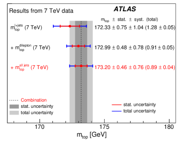
(a) ${\sqrt{s}}=7$ TeV

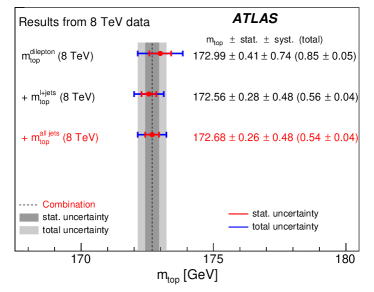
(b) ${\sqrt{s}}=8$ TeV

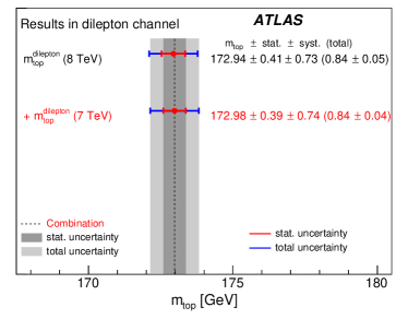
(c) $t\bar{t}\to\mathrm{dilepton}$ channel

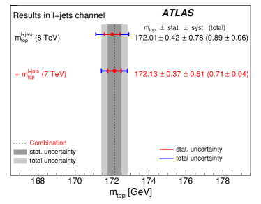
(d) $t\bar{t}\to\mathrm{lepton+jets}$ channel

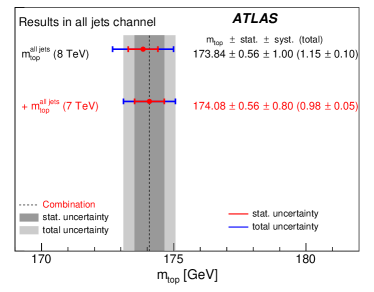
(e) $t\bar{t}\to\mathrm{all\,jets}$ channel

Figure 13: Selected combinations of the six ATLAS measurements of $m_{\mathrm{top}}$ according to importance. The figures show the combined result when successively adding results to the most precise one of a given category. Each line of this figure shows the combined result when adding the result listed to the combination, indicated by a ‘+’. The values quoted are the combined value, the statistical uncertainty, the systematic uncertainty, the total uncertainty and the uncertainty in the total uncertainty, which is statistical. Figures (a) and (b) refer to the independent combinations of the three measurements per centre-of-mass energy resulting in uncorrelated results $m_{\mathrm{top}}^{\mathrm{7TeV}}$ and $m_{\mathrm{top}}^{\mathrm{8TeV}}$. Figures (c)–(e) refer to the combination of the three correlated observables from pairs of measurements per $t\bar{t}$ decay channel, resulting in $m_{\mathrm{top}}^{\mathrm{dilepton}}$, $m_{\mathrm{top}}^{\mathrm{\ell+jets}}$ and $m_{\mathrm{top}}^{\mathrm{all\,jets}}$.

Figures 13(a) and 13(b) show the independent combinations per centre-of-mass energy. For both centre-of-mass energies, the combination is dominated by the results in the $t\bar{t}\to\mathrm{dilepton}$ and $t\bar{t}\to\mathrm{lepton+jets}$ channels. Using only those in the combinations yields combined results of $m_{\mathrm{top}}^{\mathrm{7TeV}}=172.99\,\pm\,0.48\,\mathrm{(stat)}\,\pm\,0.78\,\mathrm{(syst)}$ GeV with an uncertainty of $0.91\pm 0.05$ GeV at ${\sqrt{s}}=7$ TeV and $m_{\mathrm{top}}^{\mathrm{8TeV}}=172.56\,\pm\,0.28\,\mathrm{(stat)}\,\pm\,0.48\,\mathrm{(syst)}$ GeV with an uncertainty of $0.56\pm 0.04$ GeV at ${\sqrt{s}}=8$ TeV. At both centre-of-mass energies, the difference between the combined uncertainties of the partial and full combination is much smaller than the respective statistical precision in the total systematic uncertainties. This statistical precision is obtained from varying each systematic uncertainty within its statistical precision and repeating the combination, as explained in the main text.

Figures 13(c)–13(e) show the dependent combinations per $t\bar{t}$ decay channel. The combined result of $m_{\mathrm{top}}^{\mathrm{dilepton}}$ based only on the $t\bar{t}\to\mathrm{dilepton}$ measurement from ${\sqrt{s}}=8$ TeV data and the measurements in the other decay channels is $m_{\mathrm{top}}^{\mathrm{dilepton}}=172.94\,\pm\,0.41\,\mathrm{(stat)}\,\pm\,0.73\,\mathrm{(syst)}$ GeV with an uncertainty of $0.84\pm 0.05\leavevmode\nobreak\ \text{Ge\kern-1.00006ptV}$. As a consequence of the influence of the measurements in the other decay channels discussed in the main text, this result does not coincide with the $t\bar{t}\to\mathrm{dilepton}$ result at ${\sqrt{s}}=8$ TeV.

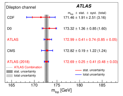
(a) $t\bar{t}\to\mathrm{dilepton}$ channel

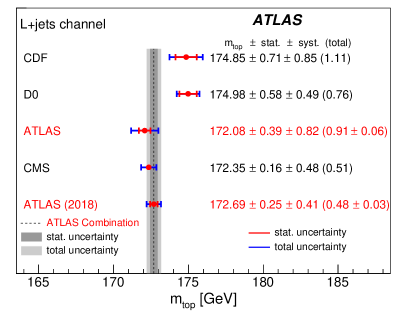
(b) $t\bar{t}\to\mathrm{lepton+jets}$ channel

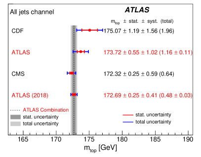
(c) $t\bar{t}\to\mathrm{all\,jets}$ channel

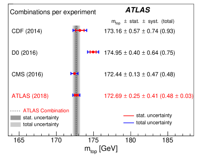
(d) Combinations

Figure 14: The most precise result of $m_{\mathrm{top}}$ per experiment in the different $t\bar{t}$ decay channels and $m_{\mathrm{top}}$ from the latest combinations performed by the individual experiments. Figure (a) shows the measurements in the $t\bar{t}\to\mathrm{dilepton}$ channel, figure (b) shows those in the $t\bar{t}\to\mathrm{lepton+jets}$ and figure (c) shows the ones in the $t\bar{t}\to\mathrm{all\,jets}$ channel. Figure (d) shows the results of $m_{\mathrm{top}}$ from the latest combination per experiment. In all figures the vertical band corresponds to the new ATLAS combined value of $m_{\mathrm{top}}$. The values quoted are the combined value, the statistical uncertainty, the systematic uncertainty, the total uncertainty and for ATLAS results also the uncertainty in the total uncertainty, which is statistical. For CDF, the separation into statistical and systematic uncertainties is different for the result in the $t\bar{t}\to\mathrm{lepton+jets}$ channel and the combination. For the former, the statistical component caused by the in situ determination of the jet scale factor is included in the statistical uncertainty, while for the latter, this uncertainty is part of the systematic uncertainty.

In Figure 14, the most precise ATLAS results of $m_{\mathrm{top}}$ per decay channel and the new ATLAS combined value of $m_{\mathrm{top}}$ are compared with the respective results from the CDF, D0 and CMS experiments.

The ATLAS Collaboration

M. Aaboud${}^{\textrm{\scriptsize 34d}}$, G. Aad${}^{\textrm{\scriptsize 99}}$, B. Abbott${}^{\textrm{\scriptsize 124}}$, O. Abdinov${}^{\textrm{\scriptsize 13,*}}$, B. Abeloos${}^{\textrm{\scriptsize 128}}$, D.K. Abhayasinghe${}^{\textrm{\scriptsize 91}}$, S.H. Abidi${}^{\textrm{\scriptsize 164}}$, O.S. AbouZeid${}^{\textrm{\scriptsize 39}}$, N.L. Abraham${}^{\textrm{\scriptsize 153}}$, H. Abramowicz${}^{\textrm{\scriptsize 158}}$, H. Abreu${}^{\textrm{\scriptsize 157}}$, Y. Abulaiti${}^{\textrm{\scriptsize 6}}$, B.S. Acharya${}^{\textrm{\scriptsize 64a,64b,o}}$, S. Adachi${}^{\textrm{\scriptsize 160}}$, L. Adam${}^{\textrm{\scriptsize 97}}$, L. Adamczyk${}^{\textrm{\scriptsize 81a}}$, J. Adelman${}^{\textrm{\scriptsize 119}}$, M. Adersberger${}^{\textrm{\scriptsize 112}}$, A. Adiguzel${}^{\textrm{\scriptsize 12c,ag}}$, T. Adye${}^{\textrm{\scriptsize 141}}$, A.A. Affolder${}^{\textrm{\scriptsize 143}}$, Y. Afik${}^{\textrm{\scriptsize 157}}$, C. Agheorghiesei${}^{\textrm{\scriptsize 27c}}$, J.A. Aguilar-Saavedra${}^{\textrm{\scriptsize 136f,136a}}$, F. Ahmadov${}^{\textrm{\scriptsize 77,ae}}$, G. Aielli${}^{\textrm{\scriptsize 71a,71b}}$, S. Akatsuka${}^{\textrm{\scriptsize 83}}$, T.P.A. Åkesson${}^{\textrm{\scriptsize 94}}$, E. Akilli${}^{\textrm{\scriptsize 52}}$, A.V. Akimov${}^{\textrm{\scriptsize 108}}$, G.L. Alberghi${}^{\textrm{\scriptsize 23b,23a}}$, J. Albert${}^{\textrm{\scriptsize 173}}$, P. Albicocco${}^{\textrm{\scriptsize 49}}$, M.J. Alconada Verzini${}^{\textrm{\scriptsize 86}}$, S. Alderweireldt${}^{\textrm{\scriptsize 117}}$, M. Aleksa${}^{\textrm{\scriptsize 35}}$, I.N. Aleksandrov${}^{\textrm{\scriptsize 77}}$, C. Alexa${}^{\textrm{\scriptsize 27b}}$, T. Alexopoulos${}^{\textrm{\scriptsize 10}}$, M. Alhroob${}^{\textrm{\scriptsize 124}}$, B. Ali${}^{\textrm{\scriptsize 138}}$, G. Alimonti${}^{\textrm{\scriptsize 66a}}$, J. Alison${}^{\textrm{\scriptsize 36}}$, S.P. Alkire${}^{\textrm{\scriptsize 145}}$, C. Allaire${}^{\textrm{\scriptsize 128}}$, B.M.M. Allbrooke${}^{\textrm{\scriptsize 153}}$, B.W. Allen${}^{\textrm{\scriptsize 127}}$, P.P. Allport${}^{\textrm{\scriptsize 21}}$, A. Aloisio${}^{\textrm{\scriptsize 67a,67b}}$, A. Alonso${}^{\textrm{\scriptsize 39}}$, F. Alonso${}^{\textrm{\scriptsize 86}}$, C. Alpigiani${}^{\textrm{\scriptsize 145}}$, A.A. Alshehri${}^{\textrm{\scriptsize 55}}$, M.I. Alstaty${}^{\textrm{\scriptsize 99}}$, B. Alvarez Gonzalez${}^{\textrm{\scriptsize 35}}$, D. Álvarez Piqueras${}^{\textrm{\scriptsize 171}}$, M.G. Alviggi${}^{\textrm{\scriptsize 67a,67b}}$, B.T. Amadio${}^{\textrm{\scriptsize 18}}$, Y. Amaral Coutinho${}^{\textrm{\scriptsize 78b}}$, A. Ambler${}^{\textrm{\scriptsize 101}}$, L. Ambroz${}^{\textrm{\scriptsize 131}}$, C. Amelung${}^{\textrm{\scriptsize 26}}$, D. Amidei${}^{\textrm{\scriptsize 103}}$, S.P. Amor Dos Santos${}^{\textrm{\scriptsize 136a,136c}}$, S. Amoroso${}^{\textrm{\scriptsize 44}}$, C.S. Amrouche${}^{\textrm{\scriptsize 52}}$, F. An${}^{\textrm{\scriptsize 76}}$, C. Anastopoulos${}^{\textrm{\scriptsize 146}}$, L.S. Ancu${}^{\textrm{\scriptsize 52}}$, N. Andari${}^{\textrm{\scriptsize 142}}$, T. Andeen${}^{\textrm{\scriptsize 11}}$, C.F. Anders${}^{\textrm{\scriptsize 59b}}$, J.K. Anders${}^{\textrm{\scriptsize 20}}$, K.J. Anderson${}^{\textrm{\scriptsize 36}}$, A. Andreazza${}^{\textrm{\scriptsize 66a,66b}}$, V. Andrei${}^{\textrm{\scriptsize 59a}}$, C.R. Anelli${}^{\textrm{\scriptsize 173}}$, S. Angelidakis${}^{\textrm{\scriptsize 37}}$, I. Angelozzi${}^{\textrm{\scriptsize 118}}$, A. Angerami${}^{\textrm{\scriptsize 38}}$, A.V. Anisenkov${}^{\textrm{\scriptsize 120b,120a}}$, A. Annovi${}^{\textrm{\scriptsize 69a}}$, C. Antel${}^{\textrm{\scriptsize 59a}}$, M.T. Anthony${}^{\textrm{\scriptsize 146}}$, M. Antonelli${}^{\textrm{\scriptsize 49}}$, D.J.A. Antrim${}^{\textrm{\scriptsize 168}}$, F. Anulli${}^{\textrm{\scriptsize 70a}}$, M. Aoki${}^{\textrm{\scriptsize 79}}$, J.A. Aparisi Pozo${}^{\textrm{\scriptsize 171}}$, L. Aperio Bella${}^{\textrm{\scriptsize 35}}$, G. Arabidze${}^{\textrm{\scriptsize 104}}$, J.P. Araque${}^{\textrm{\scriptsize 136a}}$, V. Araujo Ferraz${}^{\textrm{\scriptsize 78b}}$, R. Araujo Pereira${}^{\textrm{\scriptsize 78b}}$, A.T.H. Arce${}^{\textrm{\scriptsize 47}}$, R.E. Ardell${}^{\textrm{\scriptsize 91}}$, F.A. Arduh${}^{\textrm{\scriptsize 86}}$, J-F. Arguin${}^{\textrm{\scriptsize 107}}$, S. Argyropoulos${}^{\textrm{\scriptsize 75}}$, A.J. Armbruster${}^{\textrm{\scriptsize 35}}$, L.J. Armitage${}^{\textrm{\scriptsize 90}}$, A Armstrong${}^{\textrm{\scriptsize 168}}$, O. Arnaez${}^{\textrm{\scriptsize 164}}$, H. Arnold${}^{\textrm{\scriptsize 118}}$, M. Arratia${}^{\textrm{\scriptsize 31}}$, O. Arslan${}^{\textrm{\scriptsize 24}}$, A. Artamonov${}^{\textrm{\scriptsize 109,*}}$, G. Artoni${}^{\textrm{\scriptsize 131}}$, S. Artz${}^{\textrm{\scriptsize 97}}$, S. Asai${}^{\textrm{\scriptsize 160}}$, N. Asbah${}^{\textrm{\scriptsize 57}}$, E.M. Asimakopoulou${}^{\textrm{\scriptsize 169}}$, L. Asquith${}^{\textrm{\scriptsize 153}}$, K. Assamagan${}^{\textrm{\scriptsize 29}}$, R. Astalos${}^{\textrm{\scriptsize 28a}}$, R.J. Atkin${}^{\textrm{\scriptsize 32a}}$, M. Atkinson${}^{\textrm{\scriptsize 170}}$, N.B. Atlay${}^{\textrm{\scriptsize 148}}$, K. Augsten${}^{\textrm{\scriptsize 138}}$, G. Avolio${}^{\textrm{\scriptsize 35}}$, R. Avramidou${}^{\textrm{\scriptsize 58a}}$, M.K. Ayoub${}^{\textrm{\scriptsize 15a}}$, A.M. Azoulay${}^{\textrm{\scriptsize 165b}}$, G. Azuelos${}^{\textrm{\scriptsize 107,as}}$, A.E. Baas${}^{\textrm{\scriptsize 59a}}$, M.J. Baca${}^{\textrm{\scriptsize 21}}$, H. Bachacou${}^{\textrm{\scriptsize 142}}$, K. Bachas${}^{\textrm{\scriptsize 65a,65b}}$, M. Backes${}^{\textrm{\scriptsize 131}}$, P. Bagnaia${}^{\textrm{\scriptsize 70a,70b}}$, M. Bahmani${}^{\textrm{\scriptsize 82}}$, H. Bahrasemani${}^{\textrm{\scriptsize 149}}$, A.J. Bailey${}^{\textrm{\scriptsize 171}}$, J.T. Baines${}^{\textrm{\scriptsize 141}}$, M. Bajic${}^{\textrm{\scriptsize 39}}$, C. Bakalis${}^{\textrm{\scriptsize 10}}$, O.K. Baker${}^{\textrm{\scriptsize 180}}$, P.J. Bakker${}^{\textrm{\scriptsize 118}}$, D. Bakshi Gupta${}^{\textrm{\scriptsize 8}}$, S. Balaji${}^{\textrm{\scriptsize 154}}$, E.M. Baldin${}^{\textrm{\scriptsize 120b,120a}}$, P. Balek${}^{\textrm{\scriptsize 177}}$, F. Balli${}^{\textrm{\scriptsize 142}}$, W.K. Balunas${}^{\textrm{\scriptsize 133}}$, J. Balz${}^{\textrm{\scriptsize 97}}$, E. Banas${}^{\textrm{\scriptsize 82}}$, A. Bandyopadhyay${}^{\textrm{\scriptsize 24}}$, S. Banerjee${}^{\textrm{\scriptsize 178,k}}$, A.A.E. Bannoura${}^{\textrm{\scriptsize 179}}$, L. Barak${}^{\textrm{\scriptsize 158}}$, W.M. Barbe${}^{\textrm{\scriptsize 37}}$, E.L. Barberio${}^{\textrm{\scriptsize 102}}$, D. Barberis${}^{\textrm{\scriptsize 53b,53a}}$, M. Barbero${}^{\textrm{\scriptsize 99}}$, T. Barillari${}^{\textrm{\scriptsize 113}}$, M-S. Barisits${}^{\textrm{\scriptsize 35}}$, J. Barkeloo${}^{\textrm{\scriptsize 127}}$, T. Barklow${}^{\textrm{\scriptsize 150}}$, R. Barnea${}^{\textrm{\scriptsize 157}}$, S.L. Barnes${}^{\textrm{\scriptsize 58c}}$, B.M. Barnett${}^{\textrm{\scriptsize 141}}$, R.M. Barnett${}^{\textrm{\scriptsize 18}}$, Z. Barnovska-Blenessy${}^{\textrm{\scriptsize 58a}}$, A. Baroncelli${}^{\textrm{\scriptsize 72a}}$, G. Barone${}^{\textrm{\scriptsize 29}}$, A.J. Barr${}^{\textrm{\scriptsize 131}}$, L. Barranco Navarro${}^{\textrm{\scriptsize 171}}$, F. Barreiro${}^{\textrm{\scriptsize 96}}$, J. Barreiro Guimarães da Costa${}^{\textrm{\scriptsize 15a}}$, R. Bartoldus${}^{\textrm{\scriptsize 150}}$, A.E. Barton${}^{\textrm{\scriptsize 87}}$, P. Bartos${}^{\textrm{\scriptsize 28a}}$, A. Basalaev${}^{\textrm{\scriptsize 134}}$, A. Bassalat${}^{\textrm{\scriptsize 128}}$, R.L. Bates${}^{\textrm{\scriptsize 55}}$, S.J. Batista${}^{\textrm{\scriptsize 164}}$, S. Batlamous${}^{\textrm{\scriptsize 34e}}$, J.R. Batley${}^{\textrm{\scriptsize 31}}$, M. Battaglia${}^{\textrm{\scriptsize 143}}$, M. Bauce${}^{\textrm{\scriptsize 70a,70b}}$, F. Bauer${}^{\textrm{\scriptsize 142}}$, K.T. Bauer${}^{\textrm{\scriptsize 168}}$, H.S. Bawa${}^{\textrm{\scriptsize 150,m}}$, J.B. Beacham${}^{\textrm{\scriptsize 122}}$, T. Beau${}^{\textrm{\scriptsize 132}}$, P.H. Beauchemin${}^{\textrm{\scriptsize 167}}$, P. Bechtle${}^{\textrm{\scriptsize 24}}$, H.C. Beck${}^{\textrm{\scriptsize 51}}$, H.P. Beck${}^{\textrm{\scriptsize 20,r}}$, K. Becker${}^{\textrm{\scriptsize 50}}$, M. Becker${}^{\textrm{\scriptsize 97}}$, C. Becot${}^{\textrm{\scriptsize 44}}$, A. Beddall${}^{\textrm{\scriptsize 12d}}$, A.J. Beddall${}^{\textrm{\scriptsize 12a}}$, V.A. Bednyakov${}^{\textrm{\scriptsize 77}}$, M. Bedognetti${}^{\textrm{\scriptsize 118}}$, C.P. Bee${}^{\textrm{\scriptsize 152}}$, T.A. Beermann${}^{\textrm{\scriptsize 74}}$, M. Begalli${}^{\textrm{\scriptsize 78b}}$, M. Begel${}^{\textrm{\scriptsize 29}}$, A. Behera${}^{\textrm{\scriptsize 152}}$, J.K. Behr${}^{\textrm{\scriptsize 44}}$, A.S. Bell${}^{\textrm{\scriptsize 92}}$, G. Bella${}^{\textrm{\scriptsize 158}}$, L. Bellagamba${}^{\textrm{\scriptsize 23b}}$, A. Bellerive${}^{\textrm{\scriptsize 33}}$, M. Bellomo${}^{\textrm{\scriptsize 157}}$, P. Bellos${}^{\textrm{\scriptsize 9}}$, K. Belotskiy${}^{\textrm{\scriptsize 110}}$, N.L. Belyaev${}^{\textrm{\scriptsize 110}}$, O. Benary${}^{\textrm{\scriptsize 158,*}}$, D. Benchekroun${}^{\textrm{\scriptsize 34a}}$, M. Bender${}^{\textrm{\scriptsize 112}}$, N. Benekos${}^{\textrm{\scriptsize 10}}$, Y. Benhammou${}^{\textrm{\scriptsize 158}}$, E. Benhar Noccioli${}^{\textrm{\scriptsize 180}}$, J. Benitez${}^{\textrm{\scriptsize 75}}$, D.P. Benjamin${}^{\textrm{\scriptsize 47}}$, M. Benoit${}^{\textrm{\scriptsize 52}}$, J.R. Bensinger${}^{\textrm{\scriptsize 26}}$, S. Bentvelsen${}^{\textrm{\scriptsize 118}}$, L. Beresford${}^{\textrm{\scriptsize 131}}$, M. Beretta${}^{\textrm{\scriptsize 49}}$, D. Berge${}^{\textrm{\scriptsize 44}}$, E. Bergeaas Kuutmann${}^{\textrm{\scriptsize 169}}$, N. Berger${}^{\textrm{\scriptsize 5}}$, L.J. Bergsten${}^{\textrm{\scriptsize 26}}$, J. Beringer${}^{\textrm{\scriptsize 18}}$, S. Berlendis${}^{\textrm{\scriptsize 7}}$, N.R. Bernard${}^{\textrm{\scriptsize 100}}$, G. Bernardi${}^{\textrm{\scriptsize 132}}$, C. Bernius${}^{\textrm{\scriptsize 150}}$, F.U. Bernlochner${}^{\textrm{\scriptsize 24}}$, T. Berry${}^{\textrm{\scriptsize 91}}$, P. Berta${}^{\textrm{\scriptsize 97}}$, C. Bertella${}^{\textrm{\scriptsize 15a}}$, G. Bertoli${}^{\textrm{\scriptsize 43a,43b}}$, I.A. Bertram${}^{\textrm{\scriptsize 87}}$, G.J. Besjes${}^{\textrm{\scriptsize 39}}$, O. Bessidskaia Bylund${}^{\textrm{\scriptsize 179}}$, M. Bessner${}^{\textrm{\scriptsize 44}}$, N. Besson${}^{\textrm{\scriptsize 142}}$, A. Bethani${}^{\textrm{\scriptsize 98}}$, S. Bethke${}^{\textrm{\scriptsize 113}}$, A. Betti${}^{\textrm{\scriptsize 24}}$, A.J. Bevan${}^{\textrm{\scriptsize 90}}$, J. Beyer${}^{\textrm{\scriptsize 113}}$, R. Bi${}^{\textrm{\scriptsize 135}}$, R.M. Bianchi${}^{\textrm{\scriptsize 135}}$, O. Biebel${}^{\textrm{\scriptsize 112}}$, D. Biedermann${}^{\textrm{\scriptsize 19}}$, R. Bielski${}^{\textrm{\scriptsize 35}}$, K. Bierwagen${}^{\textrm{\scriptsize 97}}$, N.V. Biesuz${}^{\textrm{\scriptsize 69a,69b}}$, M. Biglietti${}^{\textrm{\scriptsize 72a}}$, T.R.V. Billoud${}^{\textrm{\scriptsize 107}}$, M. Bindi${}^{\textrm{\scriptsize 51}}$, A. Bingul${}^{\textrm{\scriptsize 12d}}$, C. Bini${}^{\textrm{\scriptsize 70a,70b}}$, S. Biondi${}^{\textrm{\scriptsize 23b,23a}}$, M. Birman${}^{\textrm{\scriptsize 177}}$, T. Bisanz${}^{\textrm{\scriptsize 51}}$, J.P. Biswal${}^{\textrm{\scriptsize 158}}$, C. Bittrich${}^{\textrm{\scriptsize 46}}$, D.M. Bjergaard${}^{\textrm{\scriptsize 47}}$, J.E. Black${}^{\textrm{\scriptsize 150}}$, K.M. Black${}^{\textrm{\scriptsize 25}}$, T. Blazek${}^{\textrm{\scriptsize 28a}}$, I. Bloch${}^{\textrm{\scriptsize 44}}$, C. Blocker${}^{\textrm{\scriptsize 26}}$, A. Blue${}^{\textrm{\scriptsize 55}}$, U. Blumenschein${}^{\textrm{\scriptsize 90}}$, Dr. Blunier${}^{\textrm{\scriptsize 144a}}$, G.J. Bobbink${}^{\textrm{\scriptsize 118}}$, V.S. Bobrovnikov${}^{\textrm{\scriptsize 120b,120a}}$, S.S. Bocchetta${}^{\textrm{\scriptsize 94}}$, A. Bocci${}^{\textrm{\scriptsize 47}}$, D. Boerner${}^{\textrm{\scriptsize 179}}$, D. Bogavac${}^{\textrm{\scriptsize 112}}$, A.G. Bogdanchikov${}^{\textrm{\scriptsize 120b,120a}}$, C. Bohm${}^{\textrm{\scriptsize 43a}}$, V. Boisvert${}^{\textrm{\scriptsize 91}}$, P. Bokan${}^{\textrm{\scriptsize 169}}$, T. Bold${}^{\textrm{\scriptsize 81a}}$, A.S. Boldyrev${}^{\textrm{\scriptsize 111}}$, A.E. Bolz${}^{\textrm{\scriptsize 59b}}$, M. Bomben${}^{\textrm{\scriptsize 132}}$, M. Bona${}^{\textrm{\scriptsize 90}}$, J.S. Bonilla${}^{\textrm{\scriptsize 127}}$, M. Boonekamp${}^{\textrm{\scriptsize 142}}$, A. Borisov${}^{\textrm{\scriptsize 140}}$, G. Borissov${}^{\textrm{\scriptsize 87}}$, J. Bortfeldt${}^{\textrm{\scriptsize 35}}$, D. Bortoletto${}^{\textrm{\scriptsize 131}}$, V. Bortolotto${}^{\textrm{\scriptsize 71a,71b}}$, D. Boscherini${}^{\textrm{\scriptsize 23b}}$, M. Bosman${}^{\textrm{\scriptsize 14}}$, J.D. Bossio Sola${}^{\textrm{\scriptsize 30}}$, K. Bouaouda${}^{\textrm{\scriptsize 34a}}$, J. Boudreau${}^{\textrm{\scriptsize 135}}$, E.V. Bouhova-Thacker${}^{\textrm{\scriptsize 87}}$, D. Boumediene${}^{\textrm{\scriptsize 37}}$, C. Bourdarios${}^{\textrm{\scriptsize 128}}$, S.K. Boutle${}^{\textrm{\scriptsize 55}}$, A. Boveia${}^{\textrm{\scriptsize 122}}$, J. Boyd${}^{\textrm{\scriptsize 35}}$, D. Boye${}^{\textrm{\scriptsize 32b}}$, I.R. Boyko${}^{\textrm{\scriptsize 77}}$, A.J. Bozson${}^{\textrm{\scriptsize 91}}$, J. Bracinik${}^{\textrm{\scriptsize 21}}$, N. Brahimi${}^{\textrm{\scriptsize 99}}$, A. Brandt${}^{\textrm{\scriptsize 8}}$, G. Brandt${}^{\textrm{\scriptsize 179}}$, O. Brandt${}^{\textrm{\scriptsize 59a}}$, F. Braren${}^{\textrm{\scriptsize 44}}$, U. Bratzler${}^{\textrm{\scriptsize 161}}$, B. Brau${}^{\textrm{\scriptsize 100}}$, J.E. Brau${}^{\textrm{\scriptsize 127}}$, W.D. Breaden Madden${}^{\textrm{\scriptsize 55}}$, K. Brendlinger${}^{\textrm{\scriptsize 44}}$, L. Brenner${}^{\textrm{\scriptsize 44}}$, R. Brenner${}^{\textrm{\scriptsize 169}}$, S. Bressler${}^{\textrm{\scriptsize 177}}$, B. Brickwedde${}^{\textrm{\scriptsize 97}}$, D.L. Briglin${}^{\textrm{\scriptsize 21}}$, D. Britton${}^{\textrm{\scriptsize 55}}$, D. Britzger${}^{\textrm{\scriptsize 113}}$, I. Brock${}^{\textrm{\scriptsize 24}}$, R. Brock${}^{\textrm{\scriptsize 104}}$, G. Brooijmans${}^{\textrm{\scriptsize 38}}$, T. Brooks${}^{\textrm{\scriptsize 91}}$, W.K. Brooks${}^{\textrm{\scriptsize 144b}}$, E. Brost${}^{\textrm{\scriptsize 119}}$, J.H Broughton${}^{\textrm{\scriptsize 21}}$, P.A. Bruckman de Renstrom${}^{\textrm{\scriptsize 82}}$, D. Bruncko${}^{\textrm{\scriptsize 28b}}$, A. Bruni${}^{\textrm{\scriptsize 23b}}$, G. Bruni${}^{\textrm{\scriptsize 23b}}$, L.S. Bruni${}^{\textrm{\scriptsize 118}}$, S. Bruno${}^{\textrm{\scriptsize 71a,71b}}$, B.H. Brunt${}^{\textrm{\scriptsize 31}}$, M. Bruschi${}^{\textrm{\scriptsize 23b}}$, N. Bruscino${}^{\textrm{\scriptsize 135}}$, P. Bryant${}^{\textrm{\scriptsize 36}}$, L. Bryngemark${}^{\textrm{\scriptsize 44}}$, T. Buanes${}^{\textrm{\scriptsize 17}}$, Q. Buat${}^{\textrm{\scriptsize 35}}$, P. Buchholz${}^{\textrm{\scriptsize 148}}$, A.G. Buckley${}^{\textrm{\scriptsize 55}}$, I.A. Budagov${}^{\textrm{\scriptsize 77}}$, M.K. Bugge${}^{\textrm{\scriptsize 130}}$, F. Bührer${}^{\textrm{\scriptsize 50}}$, O. Bulekov${}^{\textrm{\scriptsize 110}}$, D. Bullock${}^{\textrm{\scriptsize 8}}$, T.J. Burch${}^{\textrm{\scriptsize 119}}$, S. Burdin${}^{\textrm{\scriptsize 88}}$, C.D. Burgard${}^{\textrm{\scriptsize 118}}$, A.M. Burger${}^{\textrm{\scriptsize 5}}$, B. Burghgrave${}^{\textrm{\scriptsize 119}}$, K. Burka${}^{\textrm{\scriptsize 82}}$, S. Burke${}^{\textrm{\scriptsize 141}}$, I. Burmeister${}^{\textrm{\scriptsize 45}}$, J.T.P. Burr${}^{\textrm{\scriptsize 131}}$, V. Büscher${}^{\textrm{\scriptsize 97}}$, E. Buschmann${}^{\textrm{\scriptsize 51}}$, P. Bussey${}^{\textrm{\scriptsize 55}}$, J.M. Butler${}^{\textrm{\scriptsize 25}}$, C.M. Buttar${}^{\textrm{\scriptsize 55}}$, J.M. Butterworth${}^{\textrm{\scriptsize 92}}$, P. Butti${}^{\textrm{\scriptsize 35}}$, W. Buttinger${}^{\textrm{\scriptsize 35}}$, A. Buzatu${}^{\textrm{\scriptsize 155}}$, A.R. Buzykaev${}^{\textrm{\scriptsize 120b,120a}}$, G. Cabras${}^{\textrm{\scriptsize 23b,23a}}$, S. Cabrera Urbán${}^{\textrm{\scriptsize 171}}$, D. Caforio${}^{\textrm{\scriptsize 138}}$, H. Cai${}^{\textrm{\scriptsize 170}}$, V.M.M. Cairo${}^{\textrm{\scriptsize 2}}$, O. Cakir${}^{\textrm{\scriptsize 4a}}$, N. Calace${}^{\textrm{\scriptsize 52}}$, P. Calafiura${}^{\textrm{\scriptsize 18}}$, A. Calandri${}^{\textrm{\scriptsize 99}}$, G. Calderini${}^{\textrm{\scriptsize 132}}$, P. Calfayan${}^{\textrm{\scriptsize 63}}$, G. Callea${}^{\textrm{\scriptsize 55}}$, L.P. Caloba${}^{\textrm{\scriptsize 78b}}$, S. Calvente Lopez${}^{\textrm{\scriptsize 96}}$, D. Calvet${}^{\textrm{\scriptsize 37}}$, S. Calvet${}^{\textrm{\scriptsize 37}}$, T.P. Calvet${}^{\textrm{\scriptsize 152}}$, M. Calvetti${}^{\textrm{\scriptsize 69a,69b}}$, R. Camacho Toro${}^{\textrm{\scriptsize 132}}$, S. Camarda${}^{\textrm{\scriptsize 35}}$, D. Camarero Munoz${}^{\textrm{\scriptsize 96}}$, P. Camarri${}^{\textrm{\scriptsize 71a,71b}}$, D. Cameron${}^{\textrm{\scriptsize 130}}$, R. Caminal Armadans${}^{\textrm{\scriptsize 100}}$, C. Camincher${}^{\textrm{\scriptsize 35}}$, S. Campana${}^{\textrm{\scriptsize 35}}$, M. Campanelli${}^{\textrm{\scriptsize 92}}$, A. Camplani${}^{\textrm{\scriptsize 39}}$, A. Campoverde${}^{\textrm{\scriptsize 148}}$, V. Canale${}^{\textrm{\scriptsize 67a,67b}}$, M. Cano Bret${}^{\textrm{\scriptsize 58c}}$, J. Cantero${}^{\textrm{\scriptsize 125}}$, T. Cao${}^{\textrm{\scriptsize 158}}$, Y. Cao${}^{\textrm{\scriptsize 170}}$, M.D.M. Capeans Garrido${}^{\textrm{\scriptsize 35}}$, I. Caprini${}^{\textrm{\scriptsize 27b}}$, M. Caprini${}^{\textrm{\scriptsize 27b}}$, M. Capua${}^{\textrm{\scriptsize 40b,40a}}$, R.M. Carbone${}^{\textrm{\scriptsize 38}}$, R. Cardarelli${}^{\textrm{\scriptsize 71a}}$, F.C. Cardillo${}^{\textrm{\scriptsize 146}}$, I. Carli${}^{\textrm{\scriptsize 139}}$, T. Carli${}^{\textrm{\scriptsize 35}}$, G. Carlino${}^{\textrm{\scriptsize 67a}}$, B.T. Carlson${}^{\textrm{\scriptsize 135}}$, L. Carminati${}^{\textrm{\scriptsize 66a,66b}}$, R.M.D. Carney${}^{\textrm{\scriptsize 43a,43b}}$, S. Caron${}^{\textrm{\scriptsize 117}}$, E. Carquin${}^{\textrm{\scriptsize 144b}}$, S. Carrá${}^{\textrm{\scriptsize 66a,66b}}$, G.D. Carrillo-Montoya${}^{\textrm{\scriptsize 35}}$, D. Casadei${}^{\textrm{\scriptsize 32b}}$, M.P. Casado${}^{\textrm{\scriptsize 14,g}}$, A.F. Casha${}^{\textrm{\scriptsize 164}}$, D.W. Casper${}^{\textrm{\scriptsize 168}}$, R. Castelijn${}^{\textrm{\scriptsize 118}}$, F.L. Castillo${}^{\textrm{\scriptsize 171}}$, V. Castillo Gimenez${}^{\textrm{\scriptsize 171}}$, N.F. Castro${}^{\textrm{\scriptsize 136a,136e}}$, A. Catinaccio${}^{\textrm{\scriptsize 35}}$, J.R. Catmore${}^{\textrm{\scriptsize 130}}$, A. Cattai${}^{\textrm{\scriptsize 35}}$, J. Caudron${}^{\textrm{\scriptsize 24}}$, V. Cavaliere${}^{\textrm{\scriptsize 29}}$, E. Cavallaro${}^{\textrm{\scriptsize 14}}$, D. Cavalli${}^{\textrm{\scriptsize 66a}}$, M. Cavalli-Sforza${}^{\textrm{\scriptsize 14}}$, V. Cavasinni${}^{\textrm{\scriptsize 69a,69b}}$, E. Celebi${}^{\textrm{\scriptsize 12b}}$, F. Ceradini${}^{\textrm{\scriptsize 72a,72b}}$, L. Cerda Alberich${}^{\textrm{\scriptsize 171}}$, A.S. Cerqueira${}^{\textrm{\scriptsize 78a}}$, A. Cerri${}^{\textrm{\scriptsize 153}}$, L. Cerrito${}^{\textrm{\scriptsize 71a,71b}}$, F. Cerutti${}^{\textrm{\scriptsize 18}}$, A. Cervelli${}^{\textrm{\scriptsize 23b,23a}}$, S.A. Cetin${}^{\textrm{\scriptsize 12b}}$, A. Chafaq${}^{\textrm{\scriptsize 34a}}$, D Chakraborty${}^{\textrm{\scriptsize 119}}$, S.K. Chan${}^{\textrm{\scriptsize 57}}$, W.S. Chan${}^{\textrm{\scriptsize 118}}$, Y.L. Chan${}^{\textrm{\scriptsize 61a}}$, J.D. Chapman${}^{\textrm{\scriptsize 31}}$, B. Chargeishvili${}^{\textrm{\scriptsize 156b}}$, D.G. Charlton${}^{\textrm{\scriptsize 21}}$, C.C. Chau${}^{\textrm{\scriptsize 33}}$, C.A. Chavez Barajas${}^{\textrm{\scriptsize 153}}$, S. Che${}^{\textrm{\scriptsize 122}}$, A. Chegwidden${}^{\textrm{\scriptsize 104}}$, S. Chekanov${}^{\textrm{\scriptsize 6}}$, S.V. Chekulaev${}^{\textrm{\scriptsize 165a}}$, G.A. Chelkov${}^{\textrm{\scriptsize 77,ar}}$, M.A. Chelstowska${}^{\textrm{\scriptsize 35}}$, C. Chen${}^{\textrm{\scriptsize 58a}}$, C.H. Chen${}^{\textrm{\scriptsize 76}}$, H. Chen${}^{\textrm{\scriptsize 29}}$, J. Chen${}^{\textrm{\scriptsize 58a}}$, J. Chen${}^{\textrm{\scriptsize 38}}$, S. Chen${}^{\textrm{\scriptsize 133}}$, S.J. Chen${}^{\textrm{\scriptsize 15c}}$, X. Chen${}^{\textrm{\scriptsize 15b,aq}}$, Y. Chen${}^{\textrm{\scriptsize 80}}$, Y-H. Chen${}^{\textrm{\scriptsize 44}}$, H.C. Cheng${}^{\textrm{\scriptsize 103}}$, H.J. Cheng${}^{\textrm{\scriptsize 15d}}$, A. Cheplakov${}^{\textrm{\scriptsize 77}}$, E. Cheremushkina${}^{\textrm{\scriptsize 140}}$, R. Cherkaoui El Moursli${}^{\textrm{\scriptsize 34e}}$, E. Cheu${}^{\textrm{\scriptsize 7}}$, K. Cheung${}^{\textrm{\scriptsize 62}}$, T.J.A. Chevalérias${}^{\textrm{\scriptsize 142}}$, L. Chevalier${}^{\textrm{\scriptsize 142}}$, V. Chiarella${}^{\textrm{\scriptsize 49}}$, G. Chiarelli${}^{\textrm{\scriptsize 69a}}$, G. Chiodini${}^{\textrm{\scriptsize 65a}}$, A.S. Chisholm${}^{\textrm{\scriptsize 35,21}}$, A. Chitan${}^{\textrm{\scriptsize 27b}}$, I. Chiu${}^{\textrm{\scriptsize 160}}$, Y.H. Chiu${}^{\textrm{\scriptsize 173}}$, M.V. Chizhov${}^{\textrm{\scriptsize 77}}$, K. Choi${}^{\textrm{\scriptsize 63}}$, A.R. Chomont${}^{\textrm{\scriptsize 128}}$, S. Chouridou${}^{\textrm{\scriptsize 159}}$, Y.S. Chow${}^{\textrm{\scriptsize 118}}$, V. Christodoulou${}^{\textrm{\scriptsize 92}}$, M.C. Chu${}^{\textrm{\scriptsize 61a}}$, J. Chudoba${}^{\textrm{\scriptsize 137}}$, A.J. Chuinard${}^{\textrm{\scriptsize 101}}$, J.J. Chwastowski${}^{\textrm{\scriptsize 82}}$, L. Chytka${}^{\textrm{\scriptsize 126}}$, D. Cinca${}^{\textrm{\scriptsize 45}}$, V. Cindro${}^{\textrm{\scriptsize 89}}$, I.A. Cioară${}^{\textrm{\scriptsize 24}}$, A. Ciocio${}^{\textrm{\scriptsize 18}}$, F. Cirotto${}^{\textrm{\scriptsize 67a,67b}}$, Z.H. Citron${}^{\textrm{\scriptsize 177}}$, M. Citterio${}^{\textrm{\scriptsize 66a}}$, A. Clark${}^{\textrm{\scriptsize 52}}$, M.R. Clark${}^{\textrm{\scriptsize 38}}$, P.J. Clark${}^{\textrm{\scriptsize 48}}$, C. Clement${}^{\textrm{\scriptsize 43a,43b}}$, Y. Coadou${}^{\textrm{\scriptsize 99}}$, M. Cobal${}^{\textrm{\scriptsize 64a,64c}}$, A. Coccaro${}^{\textrm{\scriptsize 53b,53a}}$, J. Cochran${}^{\textrm{\scriptsize 76}}$, H. Cohen${}^{\textrm{\scriptsize 158}}$, A.E.C. Coimbra${}^{\textrm{\scriptsize 177}}$, L. Colasurdo${}^{\textrm{\scriptsize 117}}$, B. Cole${}^{\textrm{\scriptsize 38}}$, A.P. Colijn${}^{\textrm{\scriptsize 118}}$, J. Collot${}^{\textrm{\scriptsize 56}}$, P. Conde Muiño${}^{\textrm{\scriptsize 136a,136b}}$, E. Coniavitis${}^{\textrm{\scriptsize 50}}$, S.H. Connell${}^{\textrm{\scriptsize 32b}}$, I.A. Connelly${}^{\textrm{\scriptsize 98}}$, S. Constantinescu${}^{\textrm{\scriptsize 27b}}$, F. Conventi${}^{\textrm{\scriptsize 67a,at}}$, A.M. Cooper-Sarkar${}^{\textrm{\scriptsize 131}}$, F. Cormier${}^{\textrm{\scriptsize 172}}$, K.J.R. Cormier${}^{\textrm{\scriptsize 164}}$, L.D. Corpe${}^{\textrm{\scriptsize 92}}$, M. Corradi${}^{\textrm{\scriptsize 70a,70b}}$, E.E. Corrigan${}^{\textrm{\scriptsize 94}}$, F. Corriveau${}^{\textrm{\scriptsize 101,ac}}$, A. Cortes-Gonzalez${}^{\textrm{\scriptsize 35}}$, M.J. Costa${}^{\textrm{\scriptsize 171}}$, F. Costanza${}^{\textrm{\scriptsize 5}}$, D. Costanzo${}^{\textrm{\scriptsize 146}}$, G. Cottin${}^{\textrm{\scriptsize 31}}$, G. Cowan${}^{\textrm{\scriptsize 91}}$, B.E. Cox${}^{\textrm{\scriptsize 98}}$, J. Crane${}^{\textrm{\scriptsize 98}}$, K. Cranmer${}^{\textrm{\scriptsize 121}}$, S.J. Crawley${}^{\textrm{\scriptsize 55}}$, R.A. Creager${}^{\textrm{\scriptsize 133}}$, G. Cree${}^{\textrm{\scriptsize 33}}$, S. Crépé-Renaudin${}^{\textrm{\scriptsize 56}}$, F. Crescioli${}^{\textrm{\scriptsize 132}}$, M. Cristinziani${}^{\textrm{\scriptsize 24}}$, V. Croft${}^{\textrm{\scriptsize 121}}$, G. Crosetti${}^{\textrm{\scriptsize 40b,40a}}$, A. Cueto${}^{\textrm{\scriptsize 96}}$, T. Cuhadar Donszelmann${}^{\textrm{\scriptsize 146}}$, A.R. Cukierman${}^{\textrm{\scriptsize 150}}$, S. Czekierda${}^{\textrm{\scriptsize 82}}$, P. Czodrowski${}^{\textrm{\scriptsize 35}}$, M.J. Da Cunha Sargedas De Sousa${}^{\textrm{\scriptsize 58b}}$, C. Da Via${}^{\textrm{\scriptsize 98}}$, W. Dabrowski${}^{\textrm{\scriptsize 81a}}$, T. Dado${}^{\textrm{\scriptsize 28a,x}}$, S. Dahbi${}^{\textrm{\scriptsize 34e}}$, T. Dai${}^{\textrm{\scriptsize 103}}$, F. Dallaire${}^{\textrm{\scriptsize 107}}$, C. Dallapiccola${}^{\textrm{\scriptsize 100}}$, M. Dam${}^{\textrm{\scriptsize 39}}$, G. D’amen${}^{\textrm{\scriptsize 23b,23a}}$, J. Damp${}^{\textrm{\scriptsize 97}}$, J.R. Dandoy${}^{\textrm{\scriptsize 133}}$, M.F. Daneri${}^{\textrm{\scriptsize 30}}$, N.P. Dang${}^{\textrm{\scriptsize 178,k}}$, N.D Dann${}^{\textrm{\scriptsize 98}}$, M. Danninger${}^{\textrm{\scriptsize 172}}$, V. Dao${}^{\textrm{\scriptsize 35}}$, G. Darbo${}^{\textrm{\scriptsize 53b}}$, S. Darmora${}^{\textrm{\scriptsize 8}}$, O. Dartsi${}^{\textrm{\scriptsize 5}}$, A. Dattagupta${}^{\textrm{\scriptsize 127}}$, T. Daubney${}^{\textrm{\scriptsize 44}}$, S. D’Auria${}^{\textrm{\scriptsize 66a,66b}}$, W. Davey${}^{\textrm{\scriptsize 24}}$, C. David${}^{\textrm{\scriptsize 44}}$, T. Davidek${}^{\textrm{\scriptsize 139}}$, D.R. Davis${}^{\textrm{\scriptsize 47}}$, E. Dawe${}^{\textrm{\scriptsize 102}}$, I. Dawson${}^{\textrm{\scriptsize 146}}$, K. De${}^{\textrm{\scriptsize 8}}$, R. De Asmundis${}^{\textrm{\scriptsize 67a}}$, A. De Benedetti${}^{\textrm{\scriptsize 124}}$, M. De Beurs${}^{\textrm{\scriptsize 118}}$, S. De Castro${}^{\textrm{\scriptsize 23b,23a}}$, S. De Cecco${}^{\textrm{\scriptsize 70a,70b}}$, N. De Groot${}^{\textrm{\scriptsize 117}}$, P. de Jong${}^{\textrm{\scriptsize 118}}$, H. De la Torre${}^{\textrm{\scriptsize 104}}$, F. De Lorenzi${}^{\textrm{\scriptsize 76}}$, A. De Maria${}^{\textrm{\scriptsize 69a,69b}}$, D. De Pedis${}^{\textrm{\scriptsize 70a}}$, A. De Salvo${}^{\textrm{\scriptsize 70a}}$, U. De Sanctis${}^{\textrm{\scriptsize 71a,71b}}$, M. De Santis${}^{\textrm{\scriptsize 71a,71b}}$, A. De Santo${}^{\textrm{\scriptsize 153}}$, K. De Vasconcelos Corga${}^{\textrm{\scriptsize 99}}$, J.B. De Vivie De Regie${}^{\textrm{\scriptsize 128}}$, C. Debenedetti${}^{\textrm{\scriptsize 143}}$, D.V. Dedovich${}^{\textrm{\scriptsize 77}}$, N. Dehghanian${}^{\textrm{\scriptsize 3}}$, M. Del Gaudio${}^{\textrm{\scriptsize 40b,40a}}$, J. Del Peso${}^{\textrm{\scriptsize 96}}$, Y. Delabat Diaz${}^{\textrm{\scriptsize 44}}$, D. Delgove${}^{\textrm{\scriptsize 128}}$, F. Deliot${}^{\textrm{\scriptsize 142}}$, C.M. Delitzsch${}^{\textrm{\scriptsize 7}}$, M. Della Pietra${}^{\textrm{\scriptsize 67a,67b}}$, D. Della Volpe${}^{\textrm{\scriptsize 52}}$, A. Dell’Acqua${}^{\textrm{\scriptsize 35}}$, L. Dell’Asta${}^{\textrm{\scriptsize 25}}$, M. Delmastro${}^{\textrm{\scriptsize 5}}$, C. Delporte${}^{\textrm{\scriptsize 128}}$, P.A. Delsart${}^{\textrm{\scriptsize 56}}$, D.A. DeMarco${}^{\textrm{\scriptsize 164}}$, S. Demers${}^{\textrm{\scriptsize 180}}$, M. Demichev${}^{\textrm{\scriptsize 77}}$, S.P. Denisov${}^{\textrm{\scriptsize 140}}$, D. Denysiuk${}^{\textrm{\scriptsize 118}}$, L. D’Eramo${}^{\textrm{\scriptsize 132}}$, D. Derendarz${}^{\textrm{\scriptsize 82}}$, J.E. Derkaoui${}^{\textrm{\scriptsize 34d}}$, F. Derue${}^{\textrm{\scriptsize 132}}$, P. Dervan${}^{\textrm{\scriptsize 88}}$, K. Desch${}^{\textrm{\scriptsize 24}}$, C. Deterre${}^{\textrm{\scriptsize 44}}$, K. Dette${}^{\textrm{\scriptsize 164}}$, M.R. Devesa${}^{\textrm{\scriptsize 30}}$, P.O. Deviveiros${}^{\textrm{\scriptsize 35}}$, A. Dewhurst${}^{\textrm{\scriptsize 141}}$, S. Dhaliwal${}^{\textrm{\scriptsize 26}}$, F.A. Di Bello${}^{\textrm{\scriptsize 52}}$, A. Di Ciaccio${}^{\textrm{\scriptsize 71a,71b}}$, L. Di Ciaccio${}^{\textrm{\scriptsize 5}}$, W.K. Di Clemente${}^{\textrm{\scriptsize 133}}$, C. Di Donato${}^{\textrm{\scriptsize 67a,67b}}$, A. Di Girolamo${}^{\textrm{\scriptsize 35}}$, G. Di Gregorio${}^{\textrm{\scriptsize 69a,69b}}$, B. Di Micco${}^{\textrm{\scriptsize 72a,72b}}$, R. Di Nardo${}^{\textrm{\scriptsize 100}}$, K.F. Di Petrillo${}^{\textrm{\scriptsize 57}}$, R. Di Sipio${}^{\textrm{\scriptsize 164}}$, D. Di Valentino${}^{\textrm{\scriptsize 33}}$, C. Diaconu${}^{\textrm{\scriptsize 99}}$, M. Diamond${}^{\textrm{\scriptsize 164}}$, F.A. Dias${}^{\textrm{\scriptsize 39}}$, T. Dias Do Vale${}^{\textrm{\scriptsize 136a}}$, M.A. Diaz${}^{\textrm{\scriptsize 144a}}$, J. Dickinson${}^{\textrm{\scriptsize 18}}$, E.B. Diehl${}^{\textrm{\scriptsize 103}}$, J. Dietrich${}^{\textrm{\scriptsize 19}}$, S. Díez Cornell${}^{\textrm{\scriptsize 44}}$, A. Dimitrievska${}^{\textrm{\scriptsize 18}}$, J. Dingfelder${}^{\textrm{\scriptsize 24}}$, F. Dittus${}^{\textrm{\scriptsize 35}}$, F. Djama${}^{\textrm{\scriptsize 99}}$, T. Djobava${}^{\textrm{\scriptsize 156b}}$, J.I. Djuvsland${}^{\textrm{\scriptsize 59a}}$, M.A.B. Do Vale${}^{\textrm{\scriptsize 78c}}$, M. Dobre${}^{\textrm{\scriptsize 27b}}$, D. Dodsworth${}^{\textrm{\scriptsize 26}}$, C. Doglioni${}^{\textrm{\scriptsize 94}}$, J. Dolejsi${}^{\textrm{\scriptsize 139}}$, Z. Dolezal${}^{\textrm{\scriptsize 139}}$, M. Donadelli${}^{\textrm{\scriptsize 78d}}$, J. Donini${}^{\textrm{\scriptsize 37}}$, A. D’onofrio${}^{\textrm{\scriptsize 90}}$, M. D’Onofrio${}^{\textrm{\scriptsize 88}}$, J. Dopke${}^{\textrm{\scriptsize 141}}$, A. Doria${}^{\textrm{\scriptsize 67a}}$, M.T. Dova${}^{\textrm{\scriptsize 86}}$, A.T. Doyle${}^{\textrm{\scriptsize 55}}$, E. Drechsler${}^{\textrm{\scriptsize 51}}$, E. Dreyer${}^{\textrm{\scriptsize 149}}$, T. Dreyer${}^{\textrm{\scriptsize 51}}$, Y. Du${}^{\textrm{\scriptsize 58b}}$, F. Dubinin${}^{\textrm{\scriptsize 108}}$, M. Dubovsky${}^{\textrm{\scriptsize 28a}}$, A. Dubreuil${}^{\textrm{\scriptsize 52}}$, E. Duchovni${}^{\textrm{\scriptsize 177}}$, G. Duckeck${}^{\textrm{\scriptsize 112}}$, A. Ducourthial${}^{\textrm{\scriptsize 132}}$, O.A. Ducu${}^{\textrm{\scriptsize 107,w}}$, D. Duda${}^{\textrm{\scriptsize 113}}$, A. Dudarev${}^{\textrm{\scriptsize 35}}$, A.C. Dudder${}^{\textrm{\scriptsize 97}}$, E.M. Duffield${}^{\textrm{\scriptsize 18}}$, L. Duflot${}^{\textrm{\scriptsize 128}}$, M. Dührssen${}^{\textrm{\scriptsize 35}}$, C. Dülsen${}^{\textrm{\scriptsize 179}}$, M. Dumancic${}^{\textrm{\scriptsize 177}}$, A.E. Dumitriu${}^{\textrm{\scriptsize 27b,e}}$, A.K. Duncan${}^{\textrm{\scriptsize 55}}$, M. Dunford${}^{\textrm{\scriptsize 59a}}$, A. Duperrin${}^{\textrm{\scriptsize 99}}$, H. Duran Yildiz${}^{\textrm{\scriptsize 4a}}$, M. Düren${}^{\textrm{\scriptsize 54}}$, A. Durglishvili${}^{\textrm{\scriptsize 156b}}$, D. Duschinger${}^{\textrm{\scriptsize 46}}$, B. Dutta${}^{\textrm{\scriptsize 44}}$, D. Duvnjak${}^{\textrm{\scriptsize 1}}$, M. Dyndal${}^{\textrm{\scriptsize 44}}$, S. Dysch${}^{\textrm{\scriptsize 98}}$, B.S. Dziedzic${}^{\textrm{\scriptsize 82}}$, C. Eckardt${}^{\textrm{\scriptsize 44}}$, K.M. Ecker${}^{\textrm{\scriptsize 113}}$, R.C. Edgar${}^{\textrm{\scriptsize 103}}$, T. Eifert${}^{\textrm{\scriptsize 35}}$, G. Eigen${}^{\textrm{\scriptsize 17}}$, K. Einsweiler${}^{\textrm{\scriptsize 18}}$, T. Ekelof${}^{\textrm{\scriptsize 169}}$, M. El Kacimi${}^{\textrm{\scriptsize 34c}}$, R. El Kosseifi${}^{\textrm{\scriptsize 99}}$, V. Ellajosyula${}^{\textrm{\scriptsize 99}}$, M. Ellert${}^{\textrm{\scriptsize 169}}$, F. Ellinghaus${}^{\textrm{\scriptsize 179}}$, A.A. Elliot${}^{\textrm{\scriptsize 90}}$, N. Ellis${}^{\textrm{\scriptsize 35}}$, J. Elmsheuser${}^{\textrm{\scriptsize 29}}$, M. Elsing${}^{\textrm{\scriptsize 35}}$, D. Emeliyanov${}^{\textrm{\scriptsize 141}}$, A. Emerman${}^{\textrm{\scriptsize 38}}$, Y. Enari${}^{\textrm{\scriptsize 160}}$, J.S. Ennis${}^{\textrm{\scriptsize 175}}$, M.B. Epland${}^{\textrm{\scriptsize 47}}$, J. Erdmann${}^{\textrm{\scriptsize 45}}$, A. Ereditato${}^{\textrm{\scriptsize 20}}$, S. Errede${}^{\textrm{\scriptsize 170}}$, M. Escalier${}^{\textrm{\scriptsize 128}}$, C. Escobar${}^{\textrm{\scriptsize 171}}$, O. Estrada Pastor${}^{\textrm{\scriptsize 171}}$, A.I. Etienvre${}^{\textrm{\scriptsize 142}}$, E. Etzion${}^{\textrm{\scriptsize 158}}$, H. Evans${}^{\textrm{\scriptsize 63}}$, A. Ezhilov${}^{\textrm{\scriptsize 134}}$, M. Ezzi${}^{\textrm{\scriptsize 34e}}$, F. Fabbri${}^{\textrm{\scriptsize 55}}$, L. Fabbri${}^{\textrm{\scriptsize 23b,23a}}$, V. Fabiani${}^{\textrm{\scriptsize 117}}$, G. Facini${}^{\textrm{\scriptsize 92}}$, R.M. Faisca Rodrigues Pereira${}^{\textrm{\scriptsize 136a}}$, R.M. Fakhrutdinov${}^{\textrm{\scriptsize 140}}$, S. Falciano${}^{\textrm{\scriptsize 70a}}$, P.J. Falke${}^{\textrm{\scriptsize 5}}$, S. Falke${}^{\textrm{\scriptsize 5}}$, J. Faltova${}^{\textrm{\scriptsize 139}}$, Y. Fang${}^{\textrm{\scriptsize 15a}}$, M. Fanti${}^{\textrm{\scriptsize 66a,66b}}$, A. Farbin${}^{\textrm{\scriptsize 8}}$, A. Farilla${}^{\textrm{\scriptsize 72a}}$, E.M. Farina${}^{\textrm{\scriptsize 68a,68b}}$, T. Farooque${}^{\textrm{\scriptsize 104}}$, S. Farrell${}^{\textrm{\scriptsize 18}}$, S.M. Farrington${}^{\textrm{\scriptsize 175}}$, P. Farthouat${}^{\textrm{\scriptsize 35}}$, F. Fassi${}^{\textrm{\scriptsize 34e}}$, P. Fassnacht${}^{\textrm{\scriptsize 35}}$, D. Fassouliotis${}^{\textrm{\scriptsize 9}}$, M. Faucci Giannelli${}^{\textrm{\scriptsize 48}}$, A. Favareto${}^{\textrm{\scriptsize 53b,53a}}$, W.J. Fawcett${}^{\textrm{\scriptsize 31}}$, L. Fayard${}^{\textrm{\scriptsize 128}}$, O.L. Fedin${}^{\textrm{\scriptsize 134,p}}$, W. Fedorko${}^{\textrm{\scriptsize 172}}$, M. Feickert${}^{\textrm{\scriptsize 41}}$, S. Feigl${}^{\textrm{\scriptsize 130}}$, L. Feligioni${}^{\textrm{\scriptsize 99}}$, C. Feng${}^{\textrm{\scriptsize 58b}}$, E.J. Feng${}^{\textrm{\scriptsize 35}}$, M. Feng${}^{\textrm{\scriptsize 47}}$, M.J. Fenton${}^{\textrm{\scriptsize 55}}$, A.B. Fenyuk${}^{\textrm{\scriptsize 140}}$, L. Feremenga${}^{\textrm{\scriptsize 8}}$, J. Ferrando${}^{\textrm{\scriptsize 44}}$, A. Ferrari${}^{\textrm{\scriptsize 169}}$, P. Ferrari${}^{\textrm{\scriptsize 118}}$, R. Ferrari${}^{\textrm{\scriptsize 68a}}$, D.E. Ferreira de Lima${}^{\textrm{\scriptsize 59b}}$, A. Ferrer${}^{\textrm{\scriptsize 171}}$, D. Ferrere${}^{\textrm{\scriptsize 52}}$, C. Ferretti${}^{\textrm{\scriptsize 103}}$, F. Fiedler${}^{\textrm{\scriptsize 97}}$, A. Filipčič${}^{\textrm{\scriptsize 89}}$, F. Filthaut${}^{\textrm{\scriptsize 117}}$, K.D. Finelli${}^{\textrm{\scriptsize 25}}$, M.C.N. Fiolhais${}^{\textrm{\scriptsize 136a,136c,a}}$, L. Fiorini${}^{\textrm{\scriptsize 171}}$, C. Fischer${}^{\textrm{\scriptsize 14}}$, W.C. Fisher${}^{\textrm{\scriptsize 104}}$, N. Flaschel${}^{\textrm{\scriptsize 44}}$, I. Fleck${}^{\textrm{\scriptsize 148}}$, P. Fleischmann${}^{\textrm{\scriptsize 103}}$, R.R.M. Fletcher${}^{\textrm{\scriptsize 133}}$, T. Flick${}^{\textrm{\scriptsize 179}}$, B.M. Flierl${}^{\textrm{\scriptsize 112}}$, L.M. Flores${}^{\textrm{\scriptsize 133}}$, L.R. Flores Castillo${}^{\textrm{\scriptsize 61a}}$, F.M. Follega${}^{\textrm{\scriptsize 73a,73b}}$, N. Fomin${}^{\textrm{\scriptsize 17}}$, G.T. Forcolin${}^{\textrm{\scriptsize 73a,73b}}$, A. Formica${}^{\textrm{\scriptsize 142}}$, F.A. Förster${}^{\textrm{\scriptsize 14}}$, A.C. Forti${}^{\textrm{\scriptsize 98}}$, A.G. Foster${}^{\textrm{\scriptsize 21}}$, D. Fournier${}^{\textrm{\scriptsize 128}}$, H. Fox${}^{\textrm{\scriptsize 87}}$, S. Fracchia${}^{\textrm{\scriptsize 146}}$, P. Francavilla${}^{\textrm{\scriptsize 69a,69b}}$, M. Franchini${}^{\textrm{\scriptsize 23b,23a}}$, S. Franchino${}^{\textrm{\scriptsize 59a}}$, D. Francis${}^{\textrm{\scriptsize 35}}$, L. Franconi${}^{\textrm{\scriptsize 143}}$, M. Franklin${}^{\textrm{\scriptsize 57}}$, M. Frate${}^{\textrm{\scriptsize 168}}$, M. Fraternali${}^{\textrm{\scriptsize 68a,68b}}$, A.N. Fray${}^{\textrm{\scriptsize 90}}$, D. Freeborn${}^{\textrm{\scriptsize 92}}$, S.M. Fressard-Batraneanu${}^{\textrm{\scriptsize 35}}$, B. Freund${}^{\textrm{\scriptsize 107}}$, W.S. Freund${}^{\textrm{\scriptsize 78b}}$, E.M. Freundlich${}^{\textrm{\scriptsize 45}}$, D.C. Frizzell${}^{\textrm{\scriptsize 124}}$, D. Froidevaux${}^{\textrm{\scriptsize 35}}$, J.A. Frost${}^{\textrm{\scriptsize 131}}$, C. Fukunaga${}^{\textrm{\scriptsize 161}}$, E. Fullana Torregrosa${}^{\textrm{\scriptsize 171}}$, T. Fusayasu${}^{\textrm{\scriptsize 114}}$, J. Fuster${}^{\textrm{\scriptsize 171}}$, O. Gabizon${}^{\textrm{\scriptsize 157}}$, A. Gabrielli${}^{\textrm{\scriptsize 23b,23a}}$, A. Gabrielli${}^{\textrm{\scriptsize 18}}$, G.P. Gach${}^{\textrm{\scriptsize 81a}}$, S. Gadatsch${}^{\textrm{\scriptsize 52}}$, P. Gadow${}^{\textrm{\scriptsize 113}}$, G. Gagliardi${}^{\textrm{\scriptsize 53b,53a}}$, L.G. Gagnon${}^{\textrm{\scriptsize 107}}$, C. Galea${}^{\textrm{\scriptsize 27b}}$, B. Galhardo${}^{\textrm{\scriptsize 136a,136c}}$, E.J. Gallas${}^{\textrm{\scriptsize 131}}$, B.J. Gallop${}^{\textrm{\scriptsize 141}}$, P. Gallus${}^{\textrm{\scriptsize 138}}$, G. Galster${}^{\textrm{\scriptsize 39}}$, R. Gamboa Goni${}^{\textrm{\scriptsize 90}}$, K.K. Gan${}^{\textrm{\scriptsize 122}}$, S. Ganguly${}^{\textrm{\scriptsize 177}}$, J. Gao${}^{\textrm{\scriptsize 58a}}$, Y. Gao${}^{\textrm{\scriptsize 88}}$, Y.S. Gao${}^{\textrm{\scriptsize 150,m}}$, C. García${}^{\textrm{\scriptsize 171}}$, J.E. García Navarro${}^{\textrm{\scriptsize 171}}$, J.A. García Pascual${}^{\textrm{\scriptsize 15a}}$, M. Garcia-Sciveres${}^{\textrm{\scriptsize 18}}$, R.W. Gardner${}^{\textrm{\scriptsize 36}}$, N. Garelli${}^{\textrm{\scriptsize 150}}$, S. Gargiulo${}^{\textrm{\scriptsize 50}}$, V. Garonne${}^{\textrm{\scriptsize 130}}$, K. Gasnikova${}^{\textrm{\scriptsize 44}}$, A. Gaudiello${}^{\textrm{\scriptsize 53b,53a}}$, G. Gaudio${}^{\textrm{\scriptsize 68a}}$, I.L. Gavrilenko${}^{\textrm{\scriptsize 108}}$, A. Gavrilyuk${}^{\textrm{\scriptsize 109}}$, C. Gay${}^{\textrm{\scriptsize 172}}$, G. Gaycken${}^{\textrm{\scriptsize 24}}$, E.N. Gazis${}^{\textrm{\scriptsize 10}}$, C.N.P. Gee${}^{\textrm{\scriptsize 141}}$, J. Geisen${}^{\textrm{\scriptsize 51}}$, M. Geisen${}^{\textrm{\scriptsize 97}}$, M.P. Geisler${}^{\textrm{\scriptsize 59a}}$, K. Gellerstedt${}^{\textrm{\scriptsize 43a,43b}}$, C. Gemme${}^{\textrm{\scriptsize 53b}}$, M.H. Genest${}^{\textrm{\scriptsize 56}}$, C. Geng${}^{\textrm{\scriptsize 103}}$, S. Gentile${}^{\textrm{\scriptsize 70a,70b}}$, S. George${}^{\textrm{\scriptsize 91}}$, D. Gerbaudo${}^{\textrm{\scriptsize 14}}$, G. Gessner${}^{\textrm{\scriptsize 45}}$, S. Ghasemi${}^{\textrm{\scriptsize 148}}$, M. Ghasemi Bostanabad${}^{\textrm{\scriptsize 173}}$, M. Ghneimat${}^{\textrm{\scriptsize 24}}$, B. Giacobbe${}^{\textrm{\scriptsize 23b}}$, S. Giagu${}^{\textrm{\scriptsize 70a,70b}}$, N. Giangiacomi${}^{\textrm{\scriptsize 23b,23a}}$, P. Giannetti${}^{\textrm{\scriptsize 69a}}$, A. Giannini${}^{\textrm{\scriptsize 67a,67b}}$, S.M. Gibson${}^{\textrm{\scriptsize 91}}$, M. Gignac${}^{\textrm{\scriptsize 143}}$, D. Gillberg${}^{\textrm{\scriptsize 33}}$, G. Gilles${}^{\textrm{\scriptsize 179}}$, D.M. Gingrich${}^{\textrm{\scriptsize 3,as}}$, M.P. Giordani${}^{\textrm{\scriptsize 64a,64c}}$, F.M. Giorgi${}^{\textrm{\scriptsize 23b}}$, P.F. Giraud${}^{\textrm{\scriptsize 142}}$, P. Giromini${}^{\textrm{\scriptsize 57}}$, G. Giugliarelli${}^{\textrm{\scriptsize 64a,64c}}$, D. Giugni${}^{\textrm{\scriptsize 66a}}$, F. Giuli${}^{\textrm{\scriptsize 131}}$, M. Giulini${}^{\textrm{\scriptsize 59b}}$, S. Gkaitatzis${}^{\textrm{\scriptsize 159}}$, I. Gkialas${}^{\textrm{\scriptsize 9,j}}$, E.L. Gkougkousis${}^{\textrm{\scriptsize 14}}$, P. Gkountoumis${}^{\textrm{\scriptsize 10}}$, L.K. Gladilin${}^{\textrm{\scriptsize 111}}$, C. Glasman${}^{\textrm{\scriptsize 96}}$, J. Glatzer${}^{\textrm{\scriptsize 14}}$, P.C.F. Glaysher${}^{\textrm{\scriptsize 44}}$, A. Glazov${}^{\textrm{\scriptsize 44}}$, M. Goblirsch-Kolb${}^{\textrm{\scriptsize 26}}$, J. Godlewski${}^{\textrm{\scriptsize 82}}$, S. Goldfarb${}^{\textrm{\scriptsize 102}}$, T. Golling${}^{\textrm{\scriptsize 52}}$, D. Golubkov${}^{\textrm{\scriptsize 140}}$, A. Gomes${}^{\textrm{\scriptsize 136a,136b,136d}}$, R. Goncalves Gama${}^{\textrm{\scriptsize 78a}}$, R. Gonçalo${}^{\textrm{\scriptsize 136a}}$, G. Gonella${}^{\textrm{\scriptsize 50}}$, L. Gonella${}^{\textrm{\scriptsize 21}}$, A. Gongadze${}^{\textrm{\scriptsize 77}}$, F. Gonnella${}^{\textrm{\scriptsize 21}}$, J.L. Gonski${}^{\textrm{\scriptsize 57}}$, S. González de la Hoz${}^{\textrm{\scriptsize 171}}$, S. Gonzalez-Sevilla${}^{\textrm{\scriptsize 52}}$, L. Goossens${}^{\textrm{\scriptsize 35}}$, P.A. Gorbounov${}^{\textrm{\scriptsize 109}}$, H.A. Gordon${}^{\textrm{\scriptsize 29}}$, B. Gorini${}^{\textrm{\scriptsize 35}}$, E. Gorini${}^{\textrm{\scriptsize 65a,65b}}$, A. Gorišek${}^{\textrm{\scriptsize 89}}$, A.T. Goshaw${}^{\textrm{\scriptsize 47}}$, C. Gössling${}^{\textrm{\scriptsize 45}}$, M.I. Gostkin${}^{\textrm{\scriptsize 77}}$, C.A. Gottardo${}^{\textrm{\scriptsize 24}}$, C.R. Goudet${}^{\textrm{\scriptsize 128}}$, D. Goujdami${}^{\textrm{\scriptsize 34c}}$, A.G. Goussiou${}^{\textrm{\scriptsize 145}}$, N. Govender${}^{\textrm{\scriptsize 32b,c}}$, C. Goy${}^{\textrm{\scriptsize 5}}$, E. Gozani${}^{\textrm{\scriptsize 157}}$, I. Grabowska-Bold${}^{\textrm{\scriptsize 81a}}$, P.O.J. Gradin${}^{\textrm{\scriptsize 169}}$, E.C. Graham${}^{\textrm{\scriptsize 88}}$, J. Gramling${}^{\textrm{\scriptsize 168}}$, E. Gramstad${}^{\textrm{\scriptsize 130}}$, S. Grancagnolo${}^{\textrm{\scriptsize 19}}$, V. Gratchev${}^{\textrm{\scriptsize 134}}$, P.M. Gravila${}^{\textrm{\scriptsize 27f}}$, F.G. Gravili${}^{\textrm{\scriptsize 65a,65b}}$, C. Gray${}^{\textrm{\scriptsize 55}}$, H.M. Gray${}^{\textrm{\scriptsize 18}}$, Z.D. Greenwood${}^{\textrm{\scriptsize 93,ai}}$, C. Grefe${}^{\textrm{\scriptsize 24}}$, K. Gregersen${}^{\textrm{\scriptsize 94}}$, I.M. Gregor${}^{\textrm{\scriptsize 44}}$, P. Grenier${}^{\textrm{\scriptsize 150}}$, K. Grevtsov${}^{\textrm{\scriptsize 44}}$, N.A. Grieser${}^{\textrm{\scriptsize 124}}$, J. Griffiths${}^{\textrm{\scriptsize 8}}$, A.A. Grillo${}^{\textrm{\scriptsize 143}}$, K. Grimm${}^{\textrm{\scriptsize 150,b}}$, S. Grinstein${}^{\textrm{\scriptsize 14,y}}$, Ph. Gris${}^{\textrm{\scriptsize 37}}$, J.-F. Grivaz${}^{\textrm{\scriptsize 128}}$, S. Groh${}^{\textrm{\scriptsize 97}}$, E. Gross${}^{\textrm{\scriptsize 177}}$, J. Grosse-Knetter${}^{\textrm{\scriptsize 51}}$, G.C. Grossi${}^{\textrm{\scriptsize 93}}$, Z.J. Grout${}^{\textrm{\scriptsize 92}}$, C. Grud${}^{\textrm{\scriptsize 103}}$, A. Grummer${}^{\textrm{\scriptsize 116}}$, L. Guan${}^{\textrm{\scriptsize 103}}$, W. Guan${}^{\textrm{\scriptsize 178}}$, J. Guenther${}^{\textrm{\scriptsize 35}}$, A. Guerguichon${}^{\textrm{\scriptsize 128}}$, F. Guescini${}^{\textrm{\scriptsize 165a}}$, D. Guest${}^{\textrm{\scriptsize 168}}$, R. Gugel${}^{\textrm{\scriptsize 50}}$, B. Gui${}^{\textrm{\scriptsize 122}}$, T. Guillemin${}^{\textrm{\scriptsize 5}}$, S. Guindon${}^{\textrm{\scriptsize 35}}$, U. Gul${}^{\textrm{\scriptsize 55}}$, C. Gumpert${}^{\textrm{\scriptsize 35}}$, J. Guo${}^{\textrm{\scriptsize 58c}}$, W. Guo${}^{\textrm{\scriptsize 103}}$, Y. Guo${}^{\textrm{\scriptsize 58a,s}}$, Z. Guo${}^{\textrm{\scriptsize 99}}$, R. Gupta${}^{\textrm{\scriptsize 44}}$, S. Gurbuz${}^{\textrm{\scriptsize 12c}}$, G. Gustavino${}^{\textrm{\scriptsize 124}}$, B.J. Gutelman${}^{\textrm{\scriptsize 157}}$, P. Gutierrez${}^{\textrm{\scriptsize 124}}$, C. Gutschow${}^{\textrm{\scriptsize 92}}$, C. Guyot${}^{\textrm{\scriptsize 142}}$, M.P. Guzik${}^{\textrm{\scriptsize 81a}}$, C. Gwenlan${}^{\textrm{\scriptsize 131}}$, C.B. Gwilliam${}^{\textrm{\scriptsize 88}}$, A. Haas${}^{\textrm{\scriptsize 121}}$, C. Haber${}^{\textrm{\scriptsize 18}}$, H.K. Hadavand${}^{\textrm{\scriptsize 8}}$, N. Haddad${}^{\textrm{\scriptsize 34e}}$, A. Hadef${}^{\textrm{\scriptsize 58a}}$, S. Hageböck${}^{\textrm{\scriptsize 24}}$, M. Hagihara${}^{\textrm{\scriptsize 166}}$, H. Hakobyan${}^{\textrm{\scriptsize 181,*}}$, M. Haleem${}^{\textrm{\scriptsize 174}}$, J. Haley${}^{\textrm{\scriptsize 125}}$, G. Halladjian${}^{\textrm{\scriptsize 104}}$, G.D. Hallewell${}^{\textrm{\scriptsize 99}}$, K. Hamacher${}^{\textrm{\scriptsize 179}}$, P. Hamal${}^{\textrm{\scriptsize 126}}$, K. Hamano${}^{\textrm{\scriptsize 173}}$, A. Hamilton${}^{\textrm{\scriptsize 32a}}$, G.N. Hamity${}^{\textrm{\scriptsize 146}}$, K. Han${}^{\textrm{\scriptsize 58a,ah}}$, L. Han${}^{\textrm{\scriptsize 58a}}$, S. Han${}^{\textrm{\scriptsize 15d}}$, K. Hanagaki${}^{\textrm{\scriptsize 79,u}}$, M. Hance${}^{\textrm{\scriptsize 143}}$, D.M. Handl${}^{\textrm{\scriptsize 112}}$, B. Haney${}^{\textrm{\scriptsize 133}}$, R. Hankache${}^{\textrm{\scriptsize 132}}$, P. Hanke${}^{\textrm{\scriptsize 59a}}$, E. Hansen${}^{\textrm{\scriptsize 94}}$, J.B. Hansen${}^{\textrm{\scriptsize 39}}$, J.D. Hansen${}^{\textrm{\scriptsize 39}}$, M.C. Hansen${}^{\textrm{\scriptsize 24}}$, P.H. Hansen${}^{\textrm{\scriptsize 39}}$, K. Hara${}^{\textrm{\scriptsize 166}}$, A.S. Hard${}^{\textrm{\scriptsize 178}}$, T. Harenberg${}^{\textrm{\scriptsize 179}}$, S. Harkusha${}^{\textrm{\scriptsize 105}}$, P.F. Harrison${}^{\textrm{\scriptsize 175}}$, N.M. Hartmann${}^{\textrm{\scriptsize 112}}$, Y. Hasegawa${}^{\textrm{\scriptsize 147}}$, A. Hasib${}^{\textrm{\scriptsize 48}}$, S. Hassani${}^{\textrm{\scriptsize 142}}$, S. Haug${}^{\textrm{\scriptsize 20}}$, R. Hauser${}^{\textrm{\scriptsize 104}}$, L. Hauswald${}^{\textrm{\scriptsize 46}}$, L.B. Havener${}^{\textrm{\scriptsize 38}}$, M. Havranek${}^{\textrm{\scriptsize 138}}$, C.M. Hawkes${}^{\textrm{\scriptsize 21}}$, R.J. Hawkings${}^{\textrm{\scriptsize 35}}$, D. Hayden${}^{\textrm{\scriptsize 104}}$, C. Hayes${}^{\textrm{\scriptsize 152}}$, C.P. Hays${}^{\textrm{\scriptsize 131}}$, J.M. Hays${}^{\textrm{\scriptsize 90}}$, H.S. Hayward${}^{\textrm{\scriptsize 88}}$, S.J. Haywood${}^{\textrm{\scriptsize 141}}$, M.P. Heath${}^{\textrm{\scriptsize 48}}$, V. Hedberg${}^{\textrm{\scriptsize 94}}$, L. Heelan${}^{\textrm{\scriptsize 8}}$, S. Heer${}^{\textrm{\scriptsize 24}}$, K.K. Heidegger${}^{\textrm{\scriptsize 50}}$, J. Heilman${}^{\textrm{\scriptsize 33}}$, S. Heim${}^{\textrm{\scriptsize 44}}$, T. Heim${}^{\textrm{\scriptsize 18}}$, B. Heinemann${}^{\textrm{\scriptsize 44,an}}$, J.J. Heinrich${}^{\textrm{\scriptsize 112}}$, L. Heinrich${}^{\textrm{\scriptsize 121}}$, C. Heinz${}^{\textrm{\scriptsize 54}}$, J. Hejbal${}^{\textrm{\scriptsize 137}}$, L. Helary${}^{\textrm{\scriptsize 35}}$, A. Held${}^{\textrm{\scriptsize 172}}$, S. Hellesund${}^{\textrm{\scriptsize 130}}$, C.M. Helling${}^{\textrm{\scriptsize 143}}$, S. Hellman${}^{\textrm{\scriptsize 43a,43b}}$, C. Helsens${}^{\textrm{\scriptsize 35}}$, R.C.W. Henderson${}^{\textrm{\scriptsize 87}}$, Y. Heng${}^{\textrm{\scriptsize 178}}$, S. Henkelmann${}^{\textrm{\scriptsize 172}}$, A.M. Henriques Correia${}^{\textrm{\scriptsize 35}}$, G.H. Herbert${}^{\textrm{\scriptsize 19}}$, H. Herde${}^{\textrm{\scriptsize 26}}$, V. Herget${}^{\textrm{\scriptsize 174}}$, Y. Hernández Jiménez${}^{\textrm{\scriptsize 32c}}$, H. Herr${}^{\textrm{\scriptsize 97}}$, M.G. Herrmann${}^{\textrm{\scriptsize 112}}$, T. Herrmann${}^{\textrm{\scriptsize 46}}$, G. Herten${}^{\textrm{\scriptsize 50}}$, R. Hertenberger${}^{\textrm{\scriptsize 112}}$, L. Hervas${}^{\textrm{\scriptsize 35}}$, T.C. Herwig${}^{\textrm{\scriptsize 133}}$, G.G. Hesketh${}^{\textrm{\scriptsize 92}}$, N.P. Hessey${}^{\textrm{\scriptsize 165a}}$, A. Higashida${}^{\textrm{\scriptsize 160}}$, S. Higashino${}^{\textrm{\scriptsize 79}}$, E. Higón-Rodriguez${}^{\textrm{\scriptsize 171}}$, K. Hildebrand${}^{\textrm{\scriptsize 36}}$, E. Hill${}^{\textrm{\scriptsize 173}}$, J.C. Hill${}^{\textrm{\scriptsize 31}}$, K.K. Hill${}^{\textrm{\scriptsize 29}}$, K.H. Hiller${}^{\textrm{\scriptsize 44}}$, S.J. Hillier${}^{\textrm{\scriptsize 21}}$, M. Hils${}^{\textrm{\scriptsize 46}}$, I. Hinchliffe${}^{\textrm{\scriptsize 18}}$, M. Hirose${}^{\textrm{\scriptsize 129}}$, D. Hirschbuehl${}^{\textrm{\scriptsize 179}}$, B. Hiti${}^{\textrm{\scriptsize 89}}$, O. Hladik${}^{\textrm{\scriptsize 137}}$, D.R. Hlaluku${}^{\textrm{\scriptsize 32c}}$, X. Hoad${}^{\textrm{\scriptsize 48}}$, J. Hobbs${}^{\textrm{\scriptsize 152}}$, N. Hod${}^{\textrm{\scriptsize 165a}}$, M.C. Hodgkinson${}^{\textrm{\scriptsize 146}}$, A. Hoecker${}^{\textrm{\scriptsize 35}}$, M.R. Hoeferkamp${}^{\textrm{\scriptsize 116}}$, F. Hoenig${}^{\textrm{\scriptsize 112}}$, D. Hohn${}^{\textrm{\scriptsize 24}}$, D. Hohov${}^{\textrm{\scriptsize 128}}$, T.R. Holmes${}^{\textrm{\scriptsize 36}}$, M. Holzbock${}^{\textrm{\scriptsize 112}}$, M. Homann${}^{\textrm{\scriptsize 45}}$, B.H. Hommels${}^{\textrm{\scriptsize 31}}$, S. Honda${}^{\textrm{\scriptsize 166}}$, T. Honda${}^{\textrm{\scriptsize 79}}$, T.M. Hong${}^{\textrm{\scriptsize 135}}$, A. Hönle${}^{\textrm{\scriptsize 113}}$, B.H. Hooberman${}^{\textrm{\scriptsize 170}}$, W.H. Hopkins${}^{\textrm{\scriptsize 127}}$, Y. Horii${}^{\textrm{\scriptsize 115}}$, P. Horn${}^{\textrm{\scriptsize 46}}$, A.J. Horton${}^{\textrm{\scriptsize 149}}$, L.A. Horyn${}^{\textrm{\scriptsize 36}}$, J-Y. Hostachy${}^{\textrm{\scriptsize 56}}$, A. Hostiuc${}^{\textrm{\scriptsize 145}}$, S. Hou${}^{\textrm{\scriptsize 155}}$, A. Hoummada${}^{\textrm{\scriptsize 34a}}$, J. Howarth${}^{\textrm{\scriptsize 98}}$, J. Hoya${}^{\textrm{\scriptsize 86}}$, M. Hrabovsky${}^{\textrm{\scriptsize 126}}$, I. Hristova${}^{\textrm{\scriptsize 19}}$, J. Hrivnac${}^{\textrm{\scriptsize 128}}$, A. Hrynevich${}^{\textrm{\scriptsize 106}}$, T. Hryn’ova${}^{\textrm{\scriptsize 5}}$, P.J. Hsu${}^{\textrm{\scriptsize 62}}$, S.-C. Hsu${}^{\textrm{\scriptsize 145}}$, Q. Hu${}^{\textrm{\scriptsize 29}}$, S. Hu${}^{\textrm{\scriptsize 58c}}$, Y. Huang${}^{\textrm{\scriptsize 15a}}$, Z. Hubacek${}^{\textrm{\scriptsize 138}}$, F. Hubaut${}^{\textrm{\scriptsize 99}}$, M. Huebner${}^{\textrm{\scriptsize 24}}$, F. Huegging${}^{\textrm{\scriptsize 24}}$, T.B. Huffman${}^{\textrm{\scriptsize 131}}$, M. Huhtinen${}^{\textrm{\scriptsize 35}}$, R.F.H. Hunter${}^{\textrm{\scriptsize 33}}$, P. Huo${}^{\textrm{\scriptsize 152}}$, A.M. Hupe${}^{\textrm{\scriptsize 33}}$, N. Huseynov${}^{\textrm{\scriptsize 77,ae}}$, J. Huston${}^{\textrm{\scriptsize 104}}$, J. Huth${}^{\textrm{\scriptsize 57}}$, R. Hyneman${}^{\textrm{\scriptsize 103}}$, G. Iacobucci${}^{\textrm{\scriptsize 52}}$, G. Iakovidis${}^{\textrm{\scriptsize 29}}$, I. Ibragimov${}^{\textrm{\scriptsize 148}}$, L. Iconomidou-Fayard${}^{\textrm{\scriptsize 128}}$, Z. Idrissi${}^{\textrm{\scriptsize 34e}}$, P. Iengo${}^{\textrm{\scriptsize 35}}$, R. Ignazzi${}^{\textrm{\scriptsize 39}}$, O. Igonkina${}^{\textrm{\scriptsize 118,aa}}$, R. Iguchi${}^{\textrm{\scriptsize 160}}$, T. Iizawa${}^{\textrm{\scriptsize 52}}$, Y. Ikegami${}^{\textrm{\scriptsize 79}}$, M. Ikeno${}^{\textrm{\scriptsize 79}}$, D. Iliadis${}^{\textrm{\scriptsize 159}}$, N. Ilic${}^{\textrm{\scriptsize 150}}$, F. Iltzsche${}^{\textrm{\scriptsize 46}}$, G. Introzzi${}^{\textrm{\scriptsize 68a,68b}}$, M. Iodice${}^{\textrm{\scriptsize 72a}}$, K. Iordanidou${}^{\textrm{\scriptsize 38}}$, V. Ippolito${}^{\textrm{\scriptsize 70a,70b}}$, M.F. Isacson${}^{\textrm{\scriptsize 169}}$, N. Ishijima${}^{\textrm{\scriptsize 129}}$, M. Ishino${}^{\textrm{\scriptsize 160}}$, M. Ishitsuka${}^{\textrm{\scriptsize 162}}$, W. Islam${}^{\textrm{\scriptsize 125}}$, C. Issever${}^{\textrm{\scriptsize 131}}$, S. Istin${}^{\textrm{\scriptsize 157}}$, F. Ito${}^{\textrm{\scriptsize 166}}$, J.M. Iturbe Ponce${}^{\textrm{\scriptsize 61a}}$, R. Iuppa${}^{\textrm{\scriptsize 73a,73b}}$, A. Ivina${}^{\textrm{\scriptsize 177}}$, H. Iwasaki${}^{\textrm{\scriptsize 79}}$, J.M. Izen${}^{\textrm{\scriptsize 42}}$, V. Izzo${}^{\textrm{\scriptsize 67a}}$, P. Jacka${}^{\textrm{\scriptsize 137}}$, P. Jackson${}^{\textrm{\scriptsize 1}}$, R.M. Jacobs${}^{\textrm{\scriptsize 24}}$, V. Jain${}^{\textrm{\scriptsize 2}}$, G. Jäkel${}^{\textrm{\scriptsize 179}}$, K.B. Jakobi${}^{\textrm{\scriptsize 97}}$, K. Jakobs${}^{\textrm{\scriptsize 50}}$, S. Jakobsen${}^{\textrm{\scriptsize 74}}$, T. Jakoubek${}^{\textrm{\scriptsize 137}}$, D.O. Jamin${}^{\textrm{\scriptsize 125}}$, R. Jansky${}^{\textrm{\scriptsize 52}}$, J. Janssen${}^{\textrm{\scriptsize 24}}$, M. Janus${}^{\textrm{\scriptsize 51}}$, P.A. Janus${}^{\textrm{\scriptsize 81a}}$, G. Jarlskog${}^{\textrm{\scriptsize 94}}$, N. Javadov${}^{\textrm{\scriptsize 77,ae}}$, T. Javůrek${}^{\textrm{\scriptsize 35}}$, M. Javurkova${}^{\textrm{\scriptsize 50}}$, F. Jeanneau${}^{\textrm{\scriptsize 142}}$, L. Jeanty${}^{\textrm{\scriptsize 18}}$, J. Jejelava${}^{\textrm{\scriptsize 156a,af}}$, A. Jelinskas${}^{\textrm{\scriptsize 175}}$, P. Jenni${}^{\textrm{\scriptsize 50,d}}$, J. Jeong${}^{\textrm{\scriptsize 44}}$, N. Jeong${}^{\textrm{\scriptsize 44}}$, S. Jézéquel${}^{\textrm{\scriptsize 5}}$, H. Ji${}^{\textrm{\scriptsize 178}}$, J. Jia${}^{\textrm{\scriptsize 152}}$, H. Jiang${}^{\textrm{\scriptsize 76}}$, Y. Jiang${}^{\textrm{\scriptsize 58a}}$, Z. Jiang${}^{\textrm{\scriptsize 150,q}}$, S. Jiggins${}^{\textrm{\scriptsize 50}}$, F.A. Jimenez Morales${}^{\textrm{\scriptsize 37}}$, J. Jimenez Pena${}^{\textrm{\scriptsize 171}}$, S. Jin${}^{\textrm{\scriptsize 15c}}$, A. Jinaru${}^{\textrm{\scriptsize 27b}}$, O. Jinnouchi${}^{\textrm{\scriptsize 162}}$, H. Jivan${}^{\textrm{\scriptsize 32c}}$, P. Johansson${}^{\textrm{\scriptsize 146}}$, K.A. Johns${}^{\textrm{\scriptsize 7}}$, C.A. Johnson${}^{\textrm{\scriptsize 63}}$, W.J. Johnson${}^{\textrm{\scriptsize 145}}$, K. Jon-And${}^{\textrm{\scriptsize 43a,43b}}$, R.W.L. Jones${}^{\textrm{\scriptsize 87}}$, S.D. Jones${}^{\textrm{\scriptsize 153}}$, S. Jones${}^{\textrm{\scriptsize 7}}$, T.J. Jones${}^{\textrm{\scriptsize 88}}$, J. Jongmanns${}^{\textrm{\scriptsize 59a}}$, P.M. Jorge${}^{\textrm{\scriptsize 136a,136b}}$, J. Jovicevic${}^{\textrm{\scriptsize 165a}}$, X. Ju${}^{\textrm{\scriptsize 18}}$, J.J. Junggeburth${}^{\textrm{\scriptsize 113}}$, A. Juste Rozas${}^{\textrm{\scriptsize 14,y}}$, A. Kaczmarska${}^{\textrm{\scriptsize 82}}$, M. Kado${}^{\textrm{\scriptsize 128}}$, H. Kagan${}^{\textrm{\scriptsize 122}}$, M. Kagan${}^{\textrm{\scriptsize 150}}$, T. Kaji${}^{\textrm{\scriptsize 176}}$, E. Kajomovitz${}^{\textrm{\scriptsize 157}}$, C.W. Kalderon${}^{\textrm{\scriptsize 94}}$, A. Kaluza${}^{\textrm{\scriptsize 97}}$, S. Kama${}^{\textrm{\scriptsize 41}}$, A. Kamenshchikov${}^{\textrm{\scriptsize 140}}$, L. Kanjir${}^{\textrm{\scriptsize 89}}$, Y. Kano${}^{\textrm{\scriptsize 160}}$, V.A. Kantserov${}^{\textrm{\scriptsize 110}}$, J. Kanzaki${}^{\textrm{\scriptsize 79}}$, B. Kaplan${}^{\textrm{\scriptsize 121}}$, L.S. Kaplan${}^{\textrm{\scriptsize 178}}$, D. Kar${}^{\textrm{\scriptsize 32c}}$, M.J. Kareem${}^{\textrm{\scriptsize 165b}}$, E. Karentzos${}^{\textrm{\scriptsize 10}}$, S.N. Karpov${}^{\textrm{\scriptsize 77}}$, Z.M. Karpova${}^{\textrm{\scriptsize 77}}$, V. Kartvelishvili${}^{\textrm{\scriptsize 87}}$, A.N. Karyukhin${}^{\textrm{\scriptsize 140}}$, L. Kashif${}^{\textrm{\scriptsize 178}}$, R.D. Kass${}^{\textrm{\scriptsize 122}}$, A. Kastanas${}^{\textrm{\scriptsize 43a,43b}}$, Y. Kataoka${}^{\textrm{\scriptsize 160}}$, C. Kato${}^{\textrm{\scriptsize 58d,58c}}$, J. Katzy${}^{\textrm{\scriptsize 44}}$, K. Kawade${}^{\textrm{\scriptsize 80}}$, K. Kawagoe${}^{\textrm{\scriptsize 85}}$, T. Kawamoto${}^{\textrm{\scriptsize 160}}$, G. Kawamura${}^{\textrm{\scriptsize 51}}$, E.F. Kay${}^{\textrm{\scriptsize 88}}$, V.F. Kazanin${}^{\textrm{\scriptsize 120b,120a}}$, R. Keeler${}^{\textrm{\scriptsize 173}}$, R. Kehoe${}^{\textrm{\scriptsize 41}}$, J.S. Keller${}^{\textrm{\scriptsize 33}}$, E. Kellermann${}^{\textrm{\scriptsize 94}}$, J.J. Kempster${}^{\textrm{\scriptsize 21}}$, J. Kendrick${}^{\textrm{\scriptsize 21}}$, O. Kepka${}^{\textrm{\scriptsize 137}}$, S. Kersten${}^{\textrm{\scriptsize 179}}$, B.P. Kerševan${}^{\textrm{\scriptsize 89}}$, S. Ketabchi Haghighat${}^{\textrm{\scriptsize 164}}$, R.A. Keyes${}^{\textrm{\scriptsize 101}}$, M. Khader${}^{\textrm{\scriptsize 170}}$, F. Khalil-Zada${}^{\textrm{\scriptsize 13}}$, A. Khanov${}^{\textrm{\scriptsize 125}}$, A.G. Kharlamov${}^{\textrm{\scriptsize 120b,120a}}$, T. Kharlamova${}^{\textrm{\scriptsize 120b,120a}}$, E.E. Khoda${}^{\textrm{\scriptsize 172}}$, A. Khodinov${}^{\textrm{\scriptsize 163}}$, T.J. Khoo${}^{\textrm{\scriptsize 52}}$, E. Khramov${}^{\textrm{\scriptsize 77}}$, J. Khubua${}^{\textrm{\scriptsize 156b}}$, S. Kido${}^{\textrm{\scriptsize 80}}$, M. Kiehn${}^{\textrm{\scriptsize 52}}$, C.R. Kilby${}^{\textrm{\scriptsize 91}}$, Y.K. Kim${}^{\textrm{\scriptsize 36}}$, N. Kimura${}^{\textrm{\scriptsize 64a,64c}}$, O.M. Kind${}^{\textrm{\scriptsize 19}}$, B.T. King${}^{\textrm{\scriptsize 88}}$, D. Kirchmeier${}^{\textrm{\scriptsize 46}}$, J. Kirk${}^{\textrm{\scriptsize 141}}$, A.E. Kiryunin${}^{\textrm{\scriptsize 113}}$, T. Kishimoto${}^{\textrm{\scriptsize 160}}$, D. Kisielewska${}^{\textrm{\scriptsize 81a}}$, V. Kitali${}^{\textrm{\scriptsize 44}}$, O. Kivernyk${}^{\textrm{\scriptsize 5}}$, E. Kladiva${}^{\textrm{\scriptsize 28b,*}}$, T. Klapdor-Kleingrothaus${}^{\textrm{\scriptsize 50}}$, M.H. Klein${}^{\textrm{\scriptsize 103}}$, M. Klein${}^{\textrm{\scriptsize 88}}$, U. Klein${}^{\textrm{\scriptsize 88}}$, K. Kleinknecht${}^{\textrm{\scriptsize 97}}$, P. Klimek${}^{\textrm{\scriptsize 119}}$, A. Klimentov${}^{\textrm{\scriptsize 29}}$, T. Klingl${}^{\textrm{\scriptsize 24}}$, T. Klioutchnikova${}^{\textrm{\scriptsize 35}}$, F.F. Klitzner${}^{\textrm{\scriptsize 112}}$, P. Kluit${}^{\textrm{\scriptsize 118}}$, S. Kluth${}^{\textrm{\scriptsize 113}}$, E. Kneringer${}^{\textrm{\scriptsize 74}}$, E.B.F.G. Knoops${}^{\textrm{\scriptsize 99}}$, A. Knue${}^{\textrm{\scriptsize 50}}$, A. Kobayashi${}^{\textrm{\scriptsize 160}}$, D. Kobayashi${}^{\textrm{\scriptsize 85}}$, T. Kobayashi${}^{\textrm{\scriptsize 160}}$, M. Kobel${}^{\textrm{\scriptsize 46}}$, M. Kocian${}^{\textrm{\scriptsize 150}}$, P. Kodys${}^{\textrm{\scriptsize 139}}$, P.T. Koenig${}^{\textrm{\scriptsize 24}}$, T. Koffas${}^{\textrm{\scriptsize 33}}$, E. Koffeman${}^{\textrm{\scriptsize 118}}$, N.M. Köhler${}^{\textrm{\scriptsize 113}}$, T. Koi${}^{\textrm{\scriptsize 150}}$, M. Kolb${}^{\textrm{\scriptsize 59b}}$, I. Koletsou${}^{\textrm{\scriptsize 5}}$, T. Kondo${}^{\textrm{\scriptsize 79}}$, N. Kondrashova${}^{\textrm{\scriptsize 58c}}$, K. Köneke${}^{\textrm{\scriptsize 50}}$, A.C. König${}^{\textrm{\scriptsize 117}}$, T. Kono${}^{\textrm{\scriptsize 79}}$, R. Konoplich${}^{\textrm{\scriptsize 121,ak}}$, V. Konstantinides${}^{\textrm{\scriptsize 92}}$, N. Konstantinidis${}^{\textrm{\scriptsize 92}}$, B. Konya${}^{\textrm{\scriptsize 94}}$, R. Kopeliansky${}^{\textrm{\scriptsize 63}}$, S. Koperny${}^{\textrm{\scriptsize 81a}}$, K. Korcyl${}^{\textrm{\scriptsize 82}}$, K. Kordas${}^{\textrm{\scriptsize 159}}$, G. Koren${}^{\textrm{\scriptsize 158}}$, A. Korn${}^{\textrm{\scriptsize 92}}$, I. Korolkov${}^{\textrm{\scriptsize 14}}$, E.V. Korolkova${}^{\textrm{\scriptsize 146}}$, N. Korotkova${}^{\textrm{\scriptsize 111}}$, O. Kortner${}^{\textrm{\scriptsize 113}}$, S. Kortner${}^{\textrm{\scriptsize 113}}$, T. Kosek${}^{\textrm{\scriptsize 139}}$, V.V. Kostyukhin${}^{\textrm{\scriptsize 24}}$, A. Kotwal${}^{\textrm{\scriptsize 47}}$, A. Koulouris${}^{\textrm{\scriptsize 10}}$, A. Kourkoumeli-Charalampidi${}^{\textrm{\scriptsize 68a,68b}}$, C. Kourkoumelis${}^{\textrm{\scriptsize 9}}$, E. Kourlitis${}^{\textrm{\scriptsize 146}}$, V. Kouskoura${}^{\textrm{\scriptsize 29}}$, A.B. Kowalewska${}^{\textrm{\scriptsize 82}}$, R. Kowalewski${}^{\textrm{\scriptsize 173}}$, T.Z. Kowalski${}^{\textrm{\scriptsize 81a}}$, C. Kozakai${}^{\textrm{\scriptsize 160}}$, W. Kozanecki${}^{\textrm{\scriptsize 142}}$, A.S. Kozhin${}^{\textrm{\scriptsize 140}}$, V.A. Kramarenko${}^{\textrm{\scriptsize 111}}$, G. Kramberger${}^{\textrm{\scriptsize 89}}$, D. Krasnopevtsev${}^{\textrm{\scriptsize 58a}}$, M.W. Krasny${}^{\textrm{\scriptsize 132}}$, A. Krasznahorkay${}^{\textrm{\scriptsize 35}}$, D. Krauss${}^{\textrm{\scriptsize 113}}$, J.A. Kremer${}^{\textrm{\scriptsize 81a}}$, J. Kretzschmar${}^{\textrm{\scriptsize 88}}$, P. Krieger${}^{\textrm{\scriptsize 164}}$, K. Krizka${}^{\textrm{\scriptsize 18}}$, K. Kroeninger${}^{\textrm{\scriptsize 45}}$, H. Kroha${}^{\textrm{\scriptsize 113}}$, J. Kroll${}^{\textrm{\scriptsize 137}}$, J. Kroll${}^{\textrm{\scriptsize 133}}$, J. Krstic${}^{\textrm{\scriptsize 16}}$, U. Kruchonak${}^{\textrm{\scriptsize 77}}$, H. Krüger${}^{\textrm{\scriptsize 24}}$, N. Krumnack${}^{\textrm{\scriptsize 76}}$, M.C. Kruse${}^{\textrm{\scriptsize 47}}$, T. Kubota${}^{\textrm{\scriptsize 102}}$, S. Kuday${}^{\textrm{\scriptsize 4b}}$, J.T. Kuechler${}^{\textrm{\scriptsize 179}}$, S. Kuehn${}^{\textrm{\scriptsize 35}}$, A. Kugel${}^{\textrm{\scriptsize 59a}}$, F. Kuger${}^{\textrm{\scriptsize 174}}$, T. Kuhl${}^{\textrm{\scriptsize 44}}$, V. Kukhtin${}^{\textrm{\scriptsize 77}}$, R. Kukla${}^{\textrm{\scriptsize 99}}$, Y. Kulchitsky${}^{\textrm{\scriptsize 105}}$, S. Kuleshov${}^{\textrm{\scriptsize 144b}}$, Y.P. Kulinich${}^{\textrm{\scriptsize 170}}$, M. Kuna${}^{\textrm{\scriptsize 56}}$, T. Kunigo${}^{\textrm{\scriptsize 83}}$, A. Kupco${}^{\textrm{\scriptsize 137}}$, T. Kupfer${}^{\textrm{\scriptsize 45}}$, O. Kuprash${}^{\textrm{\scriptsize 158}}$, H. Kurashige${}^{\textrm{\scriptsize 80}}$, L.L. Kurchaninov${}^{\textrm{\scriptsize 165a}}$, Y.A. Kurochkin${}^{\textrm{\scriptsize 105}}$, A. Kurova${}^{\textrm{\scriptsize 110}}$, M.G. Kurth${}^{\textrm{\scriptsize 15d}}$, E.S. Kuwertz${}^{\textrm{\scriptsize 35}}$, M. Kuze${}^{\textrm{\scriptsize 162}}$, J. Kvita${}^{\textrm{\scriptsize 126}}$, T. Kwan${}^{\textrm{\scriptsize 101}}$, A. La Rosa${}^{\textrm{\scriptsize 113}}$, J.L. La Rosa Navarro${}^{\textrm{\scriptsize 78d}}$, L. La Rotonda${}^{\textrm{\scriptsize 40b,40a}}$, F. La Ruffa${}^{\textrm{\scriptsize 40b,40a}}$, C. Lacasta${}^{\textrm{\scriptsize 171}}$, F. Lacava${}^{\textrm{\scriptsize 70a,70b}}$, J. Lacey${}^{\textrm{\scriptsize 44}}$, D.P.J. Lack${}^{\textrm{\scriptsize 98}}$, H. Lacker${}^{\textrm{\scriptsize 19}}$, D. Lacour${}^{\textrm{\scriptsize 132}}$, E. Ladygin${}^{\textrm{\scriptsize 77}}$, R. Lafaye${}^{\textrm{\scriptsize 5}}$, B. Laforge${}^{\textrm{\scriptsize 132}}$, T. Lagouri${}^{\textrm{\scriptsize 32c}}$, S. Lai${}^{\textrm{\scriptsize 51}}$, S. Lammers${}^{\textrm{\scriptsize 63}}$, W. Lampl${}^{\textrm{\scriptsize 7}}$, E. Lançon${}^{\textrm{\scriptsize 29}}$, U. Landgraf${}^{\textrm{\scriptsize 50}}$, M.P.J. Landon${}^{\textrm{\scriptsize 90}}$, M.C. Lanfermann${}^{\textrm{\scriptsize 52}}$, V.S. Lang${}^{\textrm{\scriptsize 44}}$, J.C. Lange${}^{\textrm{\scriptsize 51}}$, R.J. Langenberg${}^{\textrm{\scriptsize 35}}$, A.J. Lankford${}^{\textrm{\scriptsize 168}}$, F. Lanni${}^{\textrm{\scriptsize 29}}$, K. Lantzsch${}^{\textrm{\scriptsize 24}}$, A. Lanza${}^{\textrm{\scriptsize 68a}}$, A. Lapertosa${}^{\textrm{\scriptsize 53b,53a}}$, S. Laplace${}^{\textrm{\scriptsize 132}}$, J.F. Laporte${}^{\textrm{\scriptsize 142}}$, T. Lari${}^{\textrm{\scriptsize 66a}}$, F. Lasagni Manghi${}^{\textrm{\scriptsize 23b,23a}}$, M. Lassnig${}^{\textrm{\scriptsize 35}}$, T.S. Lau${}^{\textrm{\scriptsize 61a}}$, A. Laudrain${}^{\textrm{\scriptsize 128}}$, M. Lavorgna${}^{\textrm{\scriptsize 67a,67b}}$, M. Lazzaroni${}^{\textrm{\scriptsize 66a,66b}}$, B. Le${}^{\textrm{\scriptsize 102}}$, O. Le Dortz${}^{\textrm{\scriptsize 132}}$, E. Le Guirriec${}^{\textrm{\scriptsize 99}}$, E.P. Le Quilleuc${}^{\textrm{\scriptsize 142}}$, M. LeBlanc${}^{\textrm{\scriptsize 7}}$, T. LeCompte${}^{\textrm{\scriptsize 6}}$, F. Ledroit-Guillon${}^{\textrm{\scriptsize 56}}$, C.A. Lee${}^{\textrm{\scriptsize 29}}$, G.R. Lee${}^{\textrm{\scriptsize 144a}}$, L. Lee${}^{\textrm{\scriptsize 57}}$, S.C. Lee${}^{\textrm{\scriptsize 155}}$, B. Lefebvre${}^{\textrm{\scriptsize 101}}$, M. Lefebvre${}^{\textrm{\scriptsize 173}}$, F. Legger${}^{\textrm{\scriptsize 112}}$, C. Leggett${}^{\textrm{\scriptsize 18}}$, K. Lehmann${}^{\textrm{\scriptsize 149}}$, N. Lehmann${}^{\textrm{\scriptsize 179}}$, G. Lehmann Miotto${}^{\textrm{\scriptsize 35}}$, W.A. Leight${}^{\textrm{\scriptsize 44}}$, A. Leisos${}^{\textrm{\scriptsize 159,v}}$, M.A.L. Leite${}^{\textrm{\scriptsize 78d}}$, R. Leitner${}^{\textrm{\scriptsize 139}}$, D. Lellouch${}^{\textrm{\scriptsize 177}}$, K.J.C. Leney${}^{\textrm{\scriptsize 92}}$, T. Lenz${}^{\textrm{\scriptsize 24}}$, B. Lenzi${}^{\textrm{\scriptsize 35}}$, R. Leone${}^{\textrm{\scriptsize 7}}$, S. Leone${}^{\textrm{\scriptsize 69a}}$, C. Leonidopoulos${}^{\textrm{\scriptsize 48}}$, G. Lerner${}^{\textrm{\scriptsize 153}}$, C. Leroy${}^{\textrm{\scriptsize 107}}$, R. Les${}^{\textrm{\scriptsize 164}}$, A.A.J. Lesage${}^{\textrm{\scriptsize 142}}$, C.G. Lester${}^{\textrm{\scriptsize 31}}$, M. Levchenko${}^{\textrm{\scriptsize 134}}$, J. Levêque${}^{\textrm{\scriptsize 5}}$, D. Levin${}^{\textrm{\scriptsize 103}}$, L.J. Levinson${}^{\textrm{\scriptsize 177}}$, D. Lewis${}^{\textrm{\scriptsize 90}}$, B. Li${}^{\textrm{\scriptsize 15b}}$, B. Li${}^{\textrm{\scriptsize 103}}$, C-Q. Li${}^{\textrm{\scriptsize 58a,aj}}$, H. Li${}^{\textrm{\scriptsize 58a}}$, H. Li${}^{\textrm{\scriptsize 58b}}$, L. Li${}^{\textrm{\scriptsize 58c}}$, M. Li${}^{\textrm{\scriptsize 15a}}$, Q. Li${}^{\textrm{\scriptsize 15d}}$, Q.Y. Li${}^{\textrm{\scriptsize 58a}}$, S. Li${}^{\textrm{\scriptsize 58d,58c}}$, X. Li${}^{\textrm{\scriptsize 58c}}$, Y. Li${}^{\textrm{\scriptsize 148}}$, Z. Liang${}^{\textrm{\scriptsize 15a}}$, B. Liberti${}^{\textrm{\scriptsize 71a}}$, A. Liblong${}^{\textrm{\scriptsize 164}}$, K. Lie${}^{\textrm{\scriptsize 61c}}$, S. Liem${}^{\textrm{\scriptsize 118}}$, A. Limosani${}^{\textrm{\scriptsize 154}}$, C.Y. Lin${}^{\textrm{\scriptsize 31}}$, K. Lin${}^{\textrm{\scriptsize 104}}$, T.H. Lin${}^{\textrm{\scriptsize 97}}$, R.A. Linck${}^{\textrm{\scriptsize 63}}$, J.H. Lindon${}^{\textrm{\scriptsize 21}}$, B.E. Lindquist${}^{\textrm{\scriptsize 152}}$, A.L. Lionti${}^{\textrm{\scriptsize 52}}$, E. Lipeles${}^{\textrm{\scriptsize 133}}$, A. Lipniacka${}^{\textrm{\scriptsize 17}}$, M. Lisovyi${}^{\textrm{\scriptsize 59b}}$, T.M. Liss${}^{\textrm{\scriptsize 170,ap}}$, A. Lister${}^{\textrm{\scriptsize 172}}$, A.M. Litke${}^{\textrm{\scriptsize 143}}$, J.D. Little${}^{\textrm{\scriptsize 8}}$, B. Liu${}^{\textrm{\scriptsize 76}}$, B.L Liu${}^{\textrm{\scriptsize 6}}$, H.B. Liu${}^{\textrm{\scriptsize 29}}$, H. Liu${}^{\textrm{\scriptsize 103}}$, J.B. Liu${}^{\textrm{\scriptsize 58a}}$, J.K.K. Liu${}^{\textrm{\scriptsize 131}}$, K. Liu${}^{\textrm{\scriptsize 132}}$, M. Liu${}^{\textrm{\scriptsize 58a}}$, P. Liu${}^{\textrm{\scriptsize 18}}$, Y. Liu${}^{\textrm{\scriptsize 15a}}$, Y.L. Liu${}^{\textrm{\scriptsize 58a}}$, Y.W. Liu${}^{\textrm{\scriptsize 58a}}$, M. Livan${}^{\textrm{\scriptsize 68a,68b}}$, A. Lleres${}^{\textrm{\scriptsize 56}}$, J. Llorente Merino${}^{\textrm{\scriptsize 15a}}$, S.L. Lloyd${}^{\textrm{\scriptsize 90}}$, C.Y. Lo${}^{\textrm{\scriptsize 61b}}$, F. Lo Sterzo${}^{\textrm{\scriptsize 41}}$, E.M. Lobodzinska${}^{\textrm{\scriptsize 44}}$, P. Loch${}^{\textrm{\scriptsize 7}}$, T. Lohse${}^{\textrm{\scriptsize 19}}$, K. Lohwasser${}^{\textrm{\scriptsize 146}}$, M. Lokajicek${}^{\textrm{\scriptsize 137}}$, J.D. Long${}^{\textrm{\scriptsize 170}}$, R.E. Long${}^{\textrm{\scriptsize 87}}$, L. Longo${}^{\textrm{\scriptsize 65a,65b}}$, K.A. Looper${}^{\textrm{\scriptsize 122}}$, J.A. Lopez${}^{\textrm{\scriptsize 144b}}$, I. Lopez Paz${}^{\textrm{\scriptsize 98}}$, A. Lopez Solis${}^{\textrm{\scriptsize 146}}$, J. Lorenz${}^{\textrm{\scriptsize 112}}$, N. Lorenzo Martinez${}^{\textrm{\scriptsize 5}}$, M. Losada${}^{\textrm{\scriptsize 22}}$, P.J. Lösel${}^{\textrm{\scriptsize 112}}$, A. Lösle${}^{\textrm{\scriptsize 50}}$, X. Lou${}^{\textrm{\scriptsize 44}}$, X. Lou${}^{\textrm{\scriptsize 15a}}$, A. Lounis${}^{\textrm{\scriptsize 128}}$, J. Love${}^{\textrm{\scriptsize 6}}$, P.A. Love${}^{\textrm{\scriptsize 87}}$, J.J. Lozano Bahilo${}^{\textrm{\scriptsize 171}}$, H. Lu${}^{\textrm{\scriptsize 61a}}$, M. Lu${}^{\textrm{\scriptsize 58a}}$, Y.J. Lu${}^{\textrm{\scriptsize 62}}$, H.J. Lubatti${}^{\textrm{\scriptsize 145}}$, C. Luci${}^{\textrm{\scriptsize 70a,70b}}$, A. Lucotte${}^{\textrm{\scriptsize 56}}$, C. Luedtke${}^{\textrm{\scriptsize 50}}$, F. Luehring${}^{\textrm{\scriptsize 63}}$, I. Luise${}^{\textrm{\scriptsize 132}}$, L. Luminari${}^{\textrm{\scriptsize 70a}}$, B. Lund-Jensen${}^{\textrm{\scriptsize 151}}$, M.S. Lutz${}^{\textrm{\scriptsize 100}}$, P.M. Luzi${}^{\textrm{\scriptsize 132}}$, D. Lynn${}^{\textrm{\scriptsize 29}}$, R. Lysak${}^{\textrm{\scriptsize 137}}$, E. Lytken${}^{\textrm{\scriptsize 94}}$, F. Lyu${}^{\textrm{\scriptsize 15a}}$, V. Lyubushkin${}^{\textrm{\scriptsize 77}}$, T. Lyubushkina${}^{\textrm{\scriptsize 77}}$, H. Ma${}^{\textrm{\scriptsize 29}}$, L.L. Ma${}^{\textrm{\scriptsize 58b}}$, Y. Ma${}^{\textrm{\scriptsize 58b}}$, G. Maccarrone${}^{\textrm{\scriptsize 49}}$, A. Macchiolo${}^{\textrm{\scriptsize 113}}$, C.M. Macdonald${}^{\textrm{\scriptsize 146}}$, J. Machado Miguens${}^{\textrm{\scriptsize 133,136b}}$, D. Madaffari${}^{\textrm{\scriptsize 171}}$, R. Madar${}^{\textrm{\scriptsize 37}}$, W.F. Mader${}^{\textrm{\scriptsize 46}}$, A. Madsen${}^{\textrm{\scriptsize 44}}$, N. Madysa${}^{\textrm{\scriptsize 46}}$, J. Maeda${}^{\textrm{\scriptsize 80}}$, K. Maekawa${}^{\textrm{\scriptsize 160}}$, S. Maeland${}^{\textrm{\scriptsize 17}}$, T. Maeno${}^{\textrm{\scriptsize 29}}$, M. Maerker${}^{\textrm{\scriptsize 46}}$, A.S. Maevskiy${}^{\textrm{\scriptsize 111}}$, V. Magerl${}^{\textrm{\scriptsize 50}}$, D.J. Mahon${}^{\textrm{\scriptsize 38}}$, C. Maidantchik${}^{\textrm{\scriptsize 78b}}$, T. Maier${}^{\textrm{\scriptsize 112}}$, A. Maio${}^{\textrm{\scriptsize 136a,136b,136d}}$, O. Majersky${}^{\textrm{\scriptsize 28a}}$, S. Majewski${}^{\textrm{\scriptsize 127}}$, Y. Makida${}^{\textrm{\scriptsize 79}}$, N. Makovec${}^{\textrm{\scriptsize 128}}$, B. Malaescu${}^{\textrm{\scriptsize 132}}$, Pa. Malecki${}^{\textrm{\scriptsize 82}}$, V.P. Maleev${}^{\textrm{\scriptsize 134}}$, F. Malek${}^{\textrm{\scriptsize 56}}$, U. Mallik${}^{\textrm{\scriptsize 75}}$, D. Malon${}^{\textrm{\scriptsize 6}}$, C. Malone${}^{\textrm{\scriptsize 31}}$, S. Maltezos${}^{\textrm{\scriptsize 10}}$, S. Malyukov${}^{\textrm{\scriptsize 35}}$, J. Mamuzic${}^{\textrm{\scriptsize 171}}$, G. Mancini${}^{\textrm{\scriptsize 49}}$, I. Mandić${}^{\textrm{\scriptsize 89}}$, J. Maneira${}^{\textrm{\scriptsize 136a}}$, L. Manhaes de Andrade Filho${}^{\textrm{\scriptsize 78a}}$, J. Manjarres Ramos${}^{\textrm{\scriptsize 46}}$, K.H. Mankinen${}^{\textrm{\scriptsize 94}}$, A. Mann${}^{\textrm{\scriptsize 112}}$, A. Manousos${}^{\textrm{\scriptsize 74}}$, B. Mansoulie${}^{\textrm{\scriptsize 142}}$, J.D. Mansour${}^{\textrm{\scriptsize 15a}}$, M. Mantoani${}^{\textrm{\scriptsize 51}}$, S. Manzoni${}^{\textrm{\scriptsize 66a,66b}}$, A. Marantis${}^{\textrm{\scriptsize 159}}$, G. Marceca${}^{\textrm{\scriptsize 30}}$, L. March${}^{\textrm{\scriptsize 52}}$, L. Marchese${}^{\textrm{\scriptsize 131}}$, G. Marchiori${}^{\textrm{\scriptsize 132}}$, M. Marcisovsky${}^{\textrm{\scriptsize 137}}$, C. Marcon${}^{\textrm{\scriptsize 94}}$, C.A. Marin Tobon${}^{\textrm{\scriptsize 35}}$, M. Marjanovic${}^{\textrm{\scriptsize 37}}$, D.E. Marley${}^{\textrm{\scriptsize 103}}$, F. Marroquim${}^{\textrm{\scriptsize 78b}}$, Z. Marshall${}^{\textrm{\scriptsize 18}}$, M.U.F Martensson${}^{\textrm{\scriptsize 169}}$, S. Marti-Garcia${}^{\textrm{\scriptsize 171}}$, C.B. Martin${}^{\textrm{\scriptsize 122}}$, T.A. Martin${}^{\textrm{\scriptsize 175}}$, V.J. Martin${}^{\textrm{\scriptsize 48}}$, B. Martin dit Latour${}^{\textrm{\scriptsize 17}}$, M. Martinez${}^{\textrm{\scriptsize 14,y}}$, V.I. Martinez Outschoorn${}^{\textrm{\scriptsize 100}}$, S. Martin-Haugh${}^{\textrm{\scriptsize 141}}$, V.S. Martoiu${}^{\textrm{\scriptsize 27b}}$, A.C. Martyniuk${}^{\textrm{\scriptsize 92}}$, A. Marzin${}^{\textrm{\scriptsize 35}}$, L. Masetti${}^{\textrm{\scriptsize 97}}$, T. Mashimo${}^{\textrm{\scriptsize 160}}$, R. Mashinistov${}^{\textrm{\scriptsize 108}}$, J. Masik${}^{\textrm{\scriptsize 98}}$, A.L. Maslennikov${}^{\textrm{\scriptsize 120b,120a}}$, L.H. Mason${}^{\textrm{\scriptsize 102}}$, L. Massa${}^{\textrm{\scriptsize 71a,71b}}$, P. Massarotti${}^{\textrm{\scriptsize 67a,67b}}$, P. Mastrandrea${}^{\textrm{\scriptsize 5}}$, A. Mastroberardino${}^{\textrm{\scriptsize 40b,40a}}$, T. Masubuchi${}^{\textrm{\scriptsize 160}}$, P. Mättig${}^{\textrm{\scriptsize 179}}$, J. Maurer${}^{\textrm{\scriptsize 27b}}$, B. Maček${}^{\textrm{\scriptsize 89}}$, S.J. Maxfield${}^{\textrm{\scriptsize 88}}$, D.A. Maximov${}^{\textrm{\scriptsize 120b,120a}}$, R. Mazini${}^{\textrm{\scriptsize 155}}$, I. Maznas${}^{\textrm{\scriptsize 159}}$, S.M. Mazza${}^{\textrm{\scriptsize 143}}$, G. Mc Goldrick${}^{\textrm{\scriptsize 164}}$, S.P. Mc Kee${}^{\textrm{\scriptsize 103}}$, A. McCarn${}^{\textrm{\scriptsize 103}}$, T.G. McCarthy${}^{\textrm{\scriptsize 113}}$, L.I. McClymont${}^{\textrm{\scriptsize 92}}$, W.P. McCormack${}^{\textrm{\scriptsize 18}}$, E.F. McDonald${}^{\textrm{\scriptsize 102}}$, J.A. Mcfayden${}^{\textrm{\scriptsize 35}}$, G. Mchedlidze${}^{\textrm{\scriptsize 51}}$, M.A. McKay${}^{\textrm{\scriptsize 41}}$, K.D. McLean${}^{\textrm{\scriptsize 173}}$, S.J. McMahon${}^{\textrm{\scriptsize 141}}$, P.C. McNamara${}^{\textrm{\scriptsize 102}}$, C.J. McNicol${}^{\textrm{\scriptsize 175}}$, R.A. McPherson${}^{\textrm{\scriptsize 173,ac}}$, J.E. Mdhluli${}^{\textrm{\scriptsize 32c}}$, Z.A. Meadows${}^{\textrm{\scriptsize 100}}$, S. Meehan${}^{\textrm{\scriptsize 145}}$, T.M. Megy${}^{\textrm{\scriptsize 50}}$, S. Mehlhase${}^{\textrm{\scriptsize 112}}$, A. Mehta${}^{\textrm{\scriptsize 88}}$, T. Meideck${}^{\textrm{\scriptsize 56}}$, B. Meirose${}^{\textrm{\scriptsize 42}}$, D. Melini${}^{\textrm{\scriptsize 171,h}}$, B.R. Mellado Garcia${}^{\textrm{\scriptsize 32c}}$, J.D. Mellenthin${}^{\textrm{\scriptsize 51}}$, M. Melo${}^{\textrm{\scriptsize 28a}}$, F. Meloni${}^{\textrm{\scriptsize 44}}$, A. Melzer${}^{\textrm{\scriptsize 24}}$, S.B. Menary${}^{\textrm{\scriptsize 98}}$, E.D. Mendes Gouveia${}^{\textrm{\scriptsize 136a}}$, L. Meng${}^{\textrm{\scriptsize 88}}$, X.T. Meng${}^{\textrm{\scriptsize 103}}$, A. Mengarelli${}^{\textrm{\scriptsize 23b,23a}}$, S. Menke${}^{\textrm{\scriptsize 113}}$, E. Meoni${}^{\textrm{\scriptsize 40b,40a}}$, S. Mergelmeyer${}^{\textrm{\scriptsize 19}}$, S.A.M. Merkt${}^{\textrm{\scriptsize 135}}$, C. Merlassino${}^{\textrm{\scriptsize 20}}$, P. Mermod${}^{\textrm{\scriptsize 52}}$, L. Merola${}^{\textrm{\scriptsize 67a,67b}}$, C. Meroni${}^{\textrm{\scriptsize 66a}}$, F.S. Merritt${}^{\textrm{\scriptsize 36}}$, A. Messina${}^{\textrm{\scriptsize 70a,70b}}$, J. Metcalfe${}^{\textrm{\scriptsize 6}}$, A.S. Mete${}^{\textrm{\scriptsize 168}}$, C. Meyer${}^{\textrm{\scriptsize 133}}$, J. Meyer${}^{\textrm{\scriptsize 157}}$, J-P. Meyer${}^{\textrm{\scriptsize 142}}$, H. Meyer Zu Theenhausen${}^{\textrm{\scriptsize 59a}}$, F. Miano${}^{\textrm{\scriptsize 153}}$, R.P. Middleton${}^{\textrm{\scriptsize 141}}$, L. Mijović${}^{\textrm{\scriptsize 48}}$, G. Mikenberg${}^{\textrm{\scriptsize 177}}$, M. Mikestikova${}^{\textrm{\scriptsize 137}}$, M. Mikuž${}^{\textrm{\scriptsize 89}}$, M. Milesi${}^{\textrm{\scriptsize 102}}$, A. Milic${}^{\textrm{\scriptsize 164}}$, D.A. Millar${}^{\textrm{\scriptsize 90}}$, D.W. Miller${}^{\textrm{\scriptsize 36}}$, A. Milov${}^{\textrm{\scriptsize 177}}$, D.A. Milstead${}^{\textrm{\scriptsize 43a,43b}}$, A.A. Minaenko${}^{\textrm{\scriptsize 140}}$, M. Miñano Moya${}^{\textrm{\scriptsize 171}}$, I.A. Minashvili${}^{\textrm{\scriptsize 156b}}$, A.I. Mincer${}^{\textrm{\scriptsize 121}}$, B. Mindur${}^{\textrm{\scriptsize 81a}}$, M. Mineev${}^{\textrm{\scriptsize 77}}$, Y. Minegishi${}^{\textrm{\scriptsize 160}}$, Y. Ming${}^{\textrm{\scriptsize 178}}$, L.M. Mir${}^{\textrm{\scriptsize 14}}$, A. Mirto${}^{\textrm{\scriptsize 65a,65b}}$, K.P. Mistry${}^{\textrm{\scriptsize 133}}$, T. Mitani${}^{\textrm{\scriptsize 176}}$, J. Mitrevski${}^{\textrm{\scriptsize 112}}$, V.A. Mitsou${}^{\textrm{\scriptsize 171}}$, M. Mittal${}^{\textrm{\scriptsize 58c}}$, A. Miucci${}^{\textrm{\scriptsize 20}}$, P.S. Miyagawa${}^{\textrm{\scriptsize 146}}$, A. Mizukami${}^{\textrm{\scriptsize 79}}$, J.U. Mjörnmark${}^{\textrm{\scriptsize 94}}$, T. Mkrtchyan${}^{\textrm{\scriptsize 181}}$, M. Mlynarikova${}^{\textrm{\scriptsize 139}}$, T. Moa${}^{\textrm{\scriptsize 43a,43b}}$, K. Mochizuki${}^{\textrm{\scriptsize 107}}$, P. Mogg${}^{\textrm{\scriptsize 50}}$, S. Mohapatra${}^{\textrm{\scriptsize 38}}$, S. Molander${}^{\textrm{\scriptsize 43a,43b}}$, R. Moles-Valls${}^{\textrm{\scriptsize 24}}$, M.C. Mondragon${}^{\textrm{\scriptsize 104}}$, K. Mönig${}^{\textrm{\scriptsize 44}}$, J. Monk${}^{\textrm{\scriptsize 39}}$, E. Monnier${}^{\textrm{\scriptsize 99}}$, A. Montalbano${}^{\textrm{\scriptsize 149}}$, J. Montejo Berlingen${}^{\textrm{\scriptsize 35}}$, F. Monticelli${}^{\textrm{\scriptsize 86}}$, S. Monzani${}^{\textrm{\scriptsize 66a}}$, N. Morange${}^{\textrm{\scriptsize 128}}$, D. Moreno${}^{\textrm{\scriptsize 22}}$, M. Moreno Llácer${}^{\textrm{\scriptsize 35}}$, P. Morettini${}^{\textrm{\scriptsize 53b}}$, M. Morgenstern${}^{\textrm{\scriptsize 118}}$, S. Morgenstern${}^{\textrm{\scriptsize 46}}$, D. Mori${}^{\textrm{\scriptsize 149}}$, M. Morii${}^{\textrm{\scriptsize 57}}$, M. Morinaga${}^{\textrm{\scriptsize 176}}$, V. Morisbak${}^{\textrm{\scriptsize 130}}$, A.K. Morley${}^{\textrm{\scriptsize 35}}$, G. Mornacchi${}^{\textrm{\scriptsize 35}}$, A.P. Morris${}^{\textrm{\scriptsize 92}}$, J.D. Morris${}^{\textrm{\scriptsize 90}}$, L. Morvaj${}^{\textrm{\scriptsize 152}}$, P. Moschovakos${}^{\textrm{\scriptsize 10}}$, M. Mosidze${}^{\textrm{\scriptsize 156b}}$, H.J. Moss${}^{\textrm{\scriptsize 146}}$, J. Moss${}^{\textrm{\scriptsize 150,n}}$, K. Motohashi${}^{\textrm{\scriptsize 162}}$, R. Mount${}^{\textrm{\scriptsize 150}}$, E. Mountricha${}^{\textrm{\scriptsize 35}}$, E.J.W. Moyse${}^{\textrm{\scriptsize 100}}$, S. Muanza${}^{\textrm{\scriptsize 99}}$, F. Mueller${}^{\textrm{\scriptsize 113}}$, J. Mueller${}^{\textrm{\scriptsize 135}}$, R.S.P. Mueller${}^{\textrm{\scriptsize 112}}$, D. Muenstermann${}^{\textrm{\scriptsize 87}}$, G.A. Mullier${}^{\textrm{\scriptsize 94}}$, F.J. Munoz Sanchez${}^{\textrm{\scriptsize 98}}$, P. Murin${}^{\textrm{\scriptsize 28b}}$, W.J. Murray${}^{\textrm{\scriptsize 175,141}}$, A. Murrone${}^{\textrm{\scriptsize 66a,66b}}$, M. Muškinja${}^{\textrm{\scriptsize 89}}$, C. Mwewa${}^{\textrm{\scriptsize 32a}}$, A.G. Myagkov${}^{\textrm{\scriptsize 140,al}}$, J. Myers${}^{\textrm{\scriptsize 127}}$, M. Myska${}^{\textrm{\scriptsize 138}}$, B.P. Nachman${}^{\textrm{\scriptsize 18}}$, O. Nackenhorst${}^{\textrm{\scriptsize 45}}$, K. Nagai${}^{\textrm{\scriptsize 131}}$, K. Nagano${}^{\textrm{\scriptsize 79}}$, Y. Nagasaka${}^{\textrm{\scriptsize 60}}$, M. Nagel${}^{\textrm{\scriptsize 50}}$, E. Nagy${}^{\textrm{\scriptsize 99}}$, A.M. Nairz${}^{\textrm{\scriptsize 35}}$, Y. Nakahama${}^{\textrm{\scriptsize 115}}$, K. Nakamura${}^{\textrm{\scriptsize 79}}$, T. Nakamura${}^{\textrm{\scriptsize 160}}$, I. Nakano${}^{\textrm{\scriptsize 123}}$, H. Nanjo${}^{\textrm{\scriptsize 129}}$, F. Napolitano${}^{\textrm{\scriptsize 59a}}$, R.F. Naranjo Garcia${}^{\textrm{\scriptsize 44}}$, R. Narayan${}^{\textrm{\scriptsize 11}}$, D.I. Narrias Villar${}^{\textrm{\scriptsize 59a}}$, I. Naryshkin${}^{\textrm{\scriptsize 134}}$, T. Naumann${}^{\textrm{\scriptsize 44}}$, G. Navarro${}^{\textrm{\scriptsize 22}}$, R. Nayyar${}^{\textrm{\scriptsize 7}}$, H.A. Neal${}^{\textrm{\scriptsize 103,*}}$, P.Y. Nechaeva${}^{\textrm{\scriptsize 108}}$, T.J. Neep${}^{\textrm{\scriptsize 142}}$, A. Negri${}^{\textrm{\scriptsize 68a,68b}}$, M. Negrini${}^{\textrm{\scriptsize 23b}}$, S. Nektarijevic${}^{\textrm{\scriptsize 117}}$, C. Nellist${}^{\textrm{\scriptsize 51}}$, M.E. Nelson${}^{\textrm{\scriptsize 131}}$, S. Nemecek${}^{\textrm{\scriptsize 137}}$, P. Nemethy${}^{\textrm{\scriptsize 121}}$, M. Nessi${}^{\textrm{\scriptsize 35,f}}$, M.S. Neubauer${}^{\textrm{\scriptsize 170}}$, M. Neumann${}^{\textrm{\scriptsize 179}}$, P.R. Newman${}^{\textrm{\scriptsize 21}}$, T.Y. Ng${}^{\textrm{\scriptsize 61c}}$, Y.S. Ng${}^{\textrm{\scriptsize 19}}$, H.D.N. Nguyen${}^{\textrm{\scriptsize 99}}$, T. Nguyen Manh${}^{\textrm{\scriptsize 107}}$, E. Nibigira${}^{\textrm{\scriptsize 37}}$, R.B. Nickerson${}^{\textrm{\scriptsize 131}}$, R. Nicolaidou${}^{\textrm{\scriptsize 142}}$, D.S. Nielsen${}^{\textrm{\scriptsize 39}}$, J. Nielsen${}^{\textrm{\scriptsize 143}}$, N. Nikiforou${}^{\textrm{\scriptsize 11}}$, V. Nikolaenko${}^{\textrm{\scriptsize 140,al}}$, I. Nikolic-Audit${}^{\textrm{\scriptsize 132}}$, K. Nikolopoulos${}^{\textrm{\scriptsize 21}}$, P. Nilsson${}^{\textrm{\scriptsize 29}}$, Y. Ninomiya${}^{\textrm{\scriptsize 79}}$, A. Nisati${}^{\textrm{\scriptsize 70a}}$, N. Nishu${}^{\textrm{\scriptsize 58c}}$, R. Nisius${}^{\textrm{\scriptsize 113}}$, I. Nitsche${}^{\textrm{\scriptsize 45}}$, T. Nitta${}^{\textrm{\scriptsize 176}}$, T. Nobe${}^{\textrm{\scriptsize 160}}$, Y. Noguchi${}^{\textrm{\scriptsize 83}}$, M. Nomachi${}^{\textrm{\scriptsize 129}}$, I. Nomidis${}^{\textrm{\scriptsize 132}}$, M.A. Nomura${}^{\textrm{\scriptsize 29}}$, T. Nooney${}^{\textrm{\scriptsize 90}}$, M. Nordberg${}^{\textrm{\scriptsize 35}}$, N. Norjoharuddeen${}^{\textrm{\scriptsize 131}}$, T. Novak${}^{\textrm{\scriptsize 89}}$, O. Novgorodova${}^{\textrm{\scriptsize 46}}$, R. Novotny${}^{\textrm{\scriptsize 138}}$, L. Nozka${}^{\textrm{\scriptsize 126}}$, K. Ntekas${}^{\textrm{\scriptsize 168}}$, E. Nurse${}^{\textrm{\scriptsize 92}}$, F. Nuti${}^{\textrm{\scriptsize 102}}$, F.G. Oakham${}^{\textrm{\scriptsize 33,as}}$, H. Oberlack${}^{\textrm{\scriptsize 113}}$, J. Ocariz${}^{\textrm{\scriptsize 132}}$, A. Ochi${}^{\textrm{\scriptsize 80}}$, I. Ochoa${}^{\textrm{\scriptsize 38}}$, J.P. Ochoa-Ricoux${}^{\textrm{\scriptsize 144a}}$, K. O’Connor${}^{\textrm{\scriptsize 26}}$, S. Oda${}^{\textrm{\scriptsize 85}}$, S. Odaka${}^{\textrm{\scriptsize 79}}$, S. Oerdek${}^{\textrm{\scriptsize 51}}$, A. Oh${}^{\textrm{\scriptsize 98}}$, S.H. Oh${}^{\textrm{\scriptsize 47}}$, C.C. Ohm${}^{\textrm{\scriptsize 151}}$, H. Oide${}^{\textrm{\scriptsize 53b,53a}}$, M.L. Ojeda${}^{\textrm{\scriptsize 164}}$, H. Okawa${}^{\textrm{\scriptsize 166}}$, Y. Okazaki${}^{\textrm{\scriptsize 83}}$, Y. Okumura${}^{\textrm{\scriptsize 160}}$, T. Okuyama${}^{\textrm{\scriptsize 79}}$, A. Olariu${}^{\textrm{\scriptsize 27b}}$, L.F. Oleiro Seabra${}^{\textrm{\scriptsize 136a}}$, S.A. Olivares Pino${}^{\textrm{\scriptsize 144a}}$, D. Oliveira Damazio${}^{\textrm{\scriptsize 29}}$, J.L. Oliver${}^{\textrm{\scriptsize 1}}$, M.J.R. Olsson${}^{\textrm{\scriptsize 36}}$, A. Olszewski${}^{\textrm{\scriptsize 82}}$, J. Olszowska${}^{\textrm{\scriptsize 82}}$, D.C. O’Neil${}^{\textrm{\scriptsize 149}}$, A. Onofre${}^{\textrm{\scriptsize 136a,136e}}$, K. Onogi${}^{\textrm{\scriptsize 115}}$, P.U.E. Onyisi${}^{\textrm{\scriptsize 11}}$, H. Oppen${}^{\textrm{\scriptsize 130}}$, M.J. Oreglia${}^{\textrm{\scriptsize 36}}$, G.E. Orellana${}^{\textrm{\scriptsize 86}}$, Y. Oren${}^{\textrm{\scriptsize 158}}$, D. Orestano${}^{\textrm{\scriptsize 72a,72b}}$, E.C. Orgill${}^{\textrm{\scriptsize 98}}$, N. Orlando${}^{\textrm{\scriptsize 61b}}$, A.A. O’Rourke${}^{\textrm{\scriptsize 44}}$, R.S. Orr${}^{\textrm{\scriptsize 164}}$, B. Osculati${}^{\textrm{\scriptsize 53b,53a,*}}$, V. O’Shea${}^{\textrm{\scriptsize 55}}$, R. Ospanov${}^{\textrm{\scriptsize 58a}}$, G. Otero y Garzon${}^{\textrm{\scriptsize 30}}$, H. Otono${}^{\textrm{\scriptsize 85}}$, M. Ouchrif${}^{\textrm{\scriptsize 34d}}$, F. Ould-Saada${}^{\textrm{\scriptsize 130}}$, A. Ouraou${}^{\textrm{\scriptsize 142}}$, Q. Ouyang${}^{\textrm{\scriptsize 15a}}$, M. Owen${}^{\textrm{\scriptsize 55}}$, R.E. Owen${}^{\textrm{\scriptsize 21}}$, V.E. Ozcan${}^{\textrm{\scriptsize 12c}}$, N. Ozturk${}^{\textrm{\scriptsize 8}}$, J. Pacalt${}^{\textrm{\scriptsize 126}}$, H.A. Pacey${}^{\textrm{\scriptsize 31}}$, K. Pachal${}^{\textrm{\scriptsize 149}}$, A. Pacheco Pages${}^{\textrm{\scriptsize 14}}$, L. Pacheco Rodriguez${}^{\textrm{\scriptsize 142}}$, C. Padilla Aranda${}^{\textrm{\scriptsize 14}}$, S. Pagan Griso${}^{\textrm{\scriptsize 18}}$, M. Paganini${}^{\textrm{\scriptsize 180}}$, G. Palacino${}^{\textrm{\scriptsize 63}}$, S. Palazzo${}^{\textrm{\scriptsize 48}}$, S. Palestini${}^{\textrm{\scriptsize 35}}$, M. Palka${}^{\textrm{\scriptsize 81b}}$, D. Pallin${}^{\textrm{\scriptsize 37}}$, I. Panagoulias${}^{\textrm{\scriptsize 10}}$, C.E. Pandini${}^{\textrm{\scriptsize 35}}$, J.G. Panduro Vazquez${}^{\textrm{\scriptsize 91}}$, P. Pani${}^{\textrm{\scriptsize 35}}$, G. Panizzo${}^{\textrm{\scriptsize 64a,64c}}$, L. Paolozzi${}^{\textrm{\scriptsize 52}}$, T.D. Papadopoulou${}^{\textrm{\scriptsize 10}}$, K. Papageorgiou${}^{\textrm{\scriptsize 9,j}}$, A. Paramonov${}^{\textrm{\scriptsize 6}}$, D. Paredes Hernandez${}^{\textrm{\scriptsize 61b}}$, S.R. Paredes Saenz${}^{\textrm{\scriptsize 131}}$, B. Parida${}^{\textrm{\scriptsize 163}}$, T.H. Park${}^{\textrm{\scriptsize 33}}$, A.J. Parker${}^{\textrm{\scriptsize 87}}$, K.A. Parker${}^{\textrm{\scriptsize 44}}$, M.A. Parker${}^{\textrm{\scriptsize 31}}$, F. Parodi${}^{\textrm{\scriptsize 53b,53a}}$, J.A. Parsons${}^{\textrm{\scriptsize 38}}$, U. Parzefall${}^{\textrm{\scriptsize 50}}$, V.R. Pascuzzi${}^{\textrm{\scriptsize 164}}$, J.M.P. Pasner${}^{\textrm{\scriptsize 143}}$, E. Pasqualucci${}^{\textrm{\scriptsize 70a}}$, S. Passaggio${}^{\textrm{\scriptsize 53b}}$, F. Pastore${}^{\textrm{\scriptsize 91}}$, P. Pasuwan${}^{\textrm{\scriptsize 43a,43b}}$, S. Pataraia${}^{\textrm{\scriptsize 97}}$, J.R. Pater${}^{\textrm{\scriptsize 98}}$, A. Pathak${}^{\textrm{\scriptsize 178,k}}$, T. Pauly${}^{\textrm{\scriptsize 35}}$, B. Pearson${}^{\textrm{\scriptsize 113}}$, M. Pedersen${}^{\textrm{\scriptsize 130}}$, L. Pedraza Diaz${}^{\textrm{\scriptsize 117}}$, R. Pedro${}^{\textrm{\scriptsize 136a,136b}}$, S.V. Peleganchuk${}^{\textrm{\scriptsize 120b,120a}}$, O. Penc${}^{\textrm{\scriptsize 137}}$, C. Peng${}^{\textrm{\scriptsize 15d}}$, H. Peng${}^{\textrm{\scriptsize 58a}}$, B.S. Peralva${}^{\textrm{\scriptsize 78a}}$, M.M. Perego${}^{\textrm{\scriptsize 128}}$, A.P. Pereira Peixoto${}^{\textrm{\scriptsize 136a}}$, D.V. Perepelitsa${}^{\textrm{\scriptsize 29}}$, F. Peri${}^{\textrm{\scriptsize 19}}$, L. Perini${}^{\textrm{\scriptsize 66a,66b}}$, H. Pernegger${}^{\textrm{\scriptsize 35}}$, S. Perrella${}^{\textrm{\scriptsize 67a,67b}}$, V.D. Peshekhonov${}^{\textrm{\scriptsize 77,*}}$, K. Peters${}^{\textrm{\scriptsize 44}}$, R.F.Y. Peters${}^{\textrm{\scriptsize 98}}$, B.A. Petersen${}^{\textrm{\scriptsize 35}}$, T.C. Petersen${}^{\textrm{\scriptsize 39}}$, E. Petit${}^{\textrm{\scriptsize 56}}$, A. Petridis${}^{\textrm{\scriptsize 1}}$, C. Petridou${}^{\textrm{\scriptsize 159}}$, P. Petroff${}^{\textrm{\scriptsize 128}}$, M. Petrov${}^{\textrm{\scriptsize 131}}$, F. Petrucci${}^{\textrm{\scriptsize 72a,72b}}$, M. Pettee${}^{\textrm{\scriptsize 180}}$, N.E. Pettersson${}^{\textrm{\scriptsize 100}}$, A. Peyaud${}^{\textrm{\scriptsize 142}}$, R. Pezoa${}^{\textrm{\scriptsize 144b}}$, T. Pham${}^{\textrm{\scriptsize 102}}$, F.H. Phillips${}^{\textrm{\scriptsize 104}}$, P.W. Phillips${}^{\textrm{\scriptsize 141}}$, M.W. Phipps${}^{\textrm{\scriptsize 170}}$, G. Piacquadio${}^{\textrm{\scriptsize 152}}$, E. Pianori${}^{\textrm{\scriptsize 18}}$, A. Picazio${}^{\textrm{\scriptsize 100}}$, M.A. Pickering${}^{\textrm{\scriptsize 131}}$, R.H. Pickles${}^{\textrm{\scriptsize 98}}$, R. Piegaia${}^{\textrm{\scriptsize 30}}$, J.E. Pilcher${}^{\textrm{\scriptsize 36}}$, A.D. Pilkington${}^{\textrm{\scriptsize 98}}$, M. Pinamonti${}^{\textrm{\scriptsize 71a,71b}}$, J.L. Pinfold${}^{\textrm{\scriptsize 3}}$, M. Pitt${}^{\textrm{\scriptsize 177}}$, L. Pizzimento${}^{\textrm{\scriptsize 71a,71b}}$, M.-A. Pleier${}^{\textrm{\scriptsize 29}}$, V. Pleskot${}^{\textrm{\scriptsize 139}}$, E. Plotnikova${}^{\textrm{\scriptsize 77}}$, D. Pluth${}^{\textrm{\scriptsize 76}}$, P. Podberezko${}^{\textrm{\scriptsize 120b,120a}}$, R. Poettgen${}^{\textrm{\scriptsize 94}}$, R. Poggi${}^{\textrm{\scriptsize 52}}$, L. Poggioli${}^{\textrm{\scriptsize 128}}$, I. Pogrebnyak${}^{\textrm{\scriptsize 104}}$, D. Pohl${}^{\textrm{\scriptsize 24}}$, I. Pokharel${}^{\textrm{\scriptsize 51}}$, G. Polesello${}^{\textrm{\scriptsize 68a}}$, A. Poley${}^{\textrm{\scriptsize 18}}$, A. Policicchio${}^{\textrm{\scriptsize 70a,70b}}$, R. Polifka${}^{\textrm{\scriptsize 35}}$, A. Polini${}^{\textrm{\scriptsize 23b}}$, C.S. Pollard${}^{\textrm{\scriptsize 44}}$, V. Polychronakos${}^{\textrm{\scriptsize 29}}$, D. Ponomarenko${}^{\textrm{\scriptsize 110}}$, L. Pontecorvo${}^{\textrm{\scriptsize 35}}$, G.A. Popeneciu${}^{\textrm{\scriptsize 27d}}$, D.M. Portillo Quintero${}^{\textrm{\scriptsize 132}}$, S. Pospisil${}^{\textrm{\scriptsize 138}}$, K. Potamianos${}^{\textrm{\scriptsize 44}}$, I.N. Potrap${}^{\textrm{\scriptsize 77}}$, C.J. Potter${}^{\textrm{\scriptsize 31}}$, H. Potti${}^{\textrm{\scriptsize 11}}$, T. Poulsen${}^{\textrm{\scriptsize 94}}$, J. Poveda${}^{\textrm{\scriptsize 35}}$, T.D. Powell${}^{\textrm{\scriptsize 146}}$, M.E. Pozo Astigarraga${}^{\textrm{\scriptsize 35}}$, P. Pralavorio${}^{\textrm{\scriptsize 99}}$, S. Prell${}^{\textrm{\scriptsize 76}}$, D. Price${}^{\textrm{\scriptsize 98}}$, M. Primavera${}^{\textrm{\scriptsize 65a}}$, S. Prince${}^{\textrm{\scriptsize 101}}$, N. Proklova${}^{\textrm{\scriptsize 110}}$, K. Prokofiev${}^{\textrm{\scriptsize 61c}}$, F. Prokoshin${}^{\textrm{\scriptsize 144b}}$, S. Protopopescu${}^{\textrm{\scriptsize 29}}$, J. Proudfoot${}^{\textrm{\scriptsize 6}}$, M. Przybycien${}^{\textrm{\scriptsize 81a}}$, A. Puri${}^{\textrm{\scriptsize 170}}$, P. Puzo${}^{\textrm{\scriptsize 128}}$, J. Qian${}^{\textrm{\scriptsize 103}}$, Y. Qin${}^{\textrm{\scriptsize 98}}$, A. Quadt${}^{\textrm{\scriptsize 51}}$, M. Queitsch-Maitland${}^{\textrm{\scriptsize 44}}$, A. Qureshi${}^{\textrm{\scriptsize 1}}$, P. Rados${}^{\textrm{\scriptsize 102}}$, F. Ragusa${}^{\textrm{\scriptsize 66a,66b}}$, G. Rahal${}^{\textrm{\scriptsize 95}}$, J.A. Raine${}^{\textrm{\scriptsize 52}}$, S. Rajagopalan${}^{\textrm{\scriptsize 29}}$, A. Ramirez Morales${}^{\textrm{\scriptsize 90}}$, T. Rashid${}^{\textrm{\scriptsize 128}}$, S. Raspopov${}^{\textrm{\scriptsize 5}}$, M.G. Ratti${}^{\textrm{\scriptsize 66a,66b}}$, D.M. Rauch${}^{\textrm{\scriptsize 44}}$, F. Rauscher${}^{\textrm{\scriptsize 112}}$, S. Rave${}^{\textrm{\scriptsize 97}}$, B. Ravina${}^{\textrm{\scriptsize 146}}$, I. Ravinovich${}^{\textrm{\scriptsize 177}}$, J.H. Rawling${}^{\textrm{\scriptsize 98}}$, M. Raymond${}^{\textrm{\scriptsize 35}}$, A.L. Read${}^{\textrm{\scriptsize 130}}$, N.P. Readioff${}^{\textrm{\scriptsize 56}}$, M. Reale${}^{\textrm{\scriptsize 65a,65b}}$, D.M. Rebuzzi${}^{\textrm{\scriptsize 68a,68b}}$, A. Redelbach${}^{\textrm{\scriptsize 174}}$, G. Redlinger${}^{\textrm{\scriptsize 29}}$, R. Reece${}^{\textrm{\scriptsize 143}}$, R.G. Reed${}^{\textrm{\scriptsize 32c}}$, K. Reeves${}^{\textrm{\scriptsize 42}}$, L. Rehnisch${}^{\textrm{\scriptsize 19}}$, J. Reichert${}^{\textrm{\scriptsize 133}}$, D. Reikher${}^{\textrm{\scriptsize 158}}$, A. Reiss${}^{\textrm{\scriptsize 97}}$, C. Rembser${}^{\textrm{\scriptsize 35}}$, H. Ren${}^{\textrm{\scriptsize 15d}}$, M. Rescigno${}^{\textrm{\scriptsize 70a}}$, S. Resconi${}^{\textrm{\scriptsize 66a}}$, E.D. Resseguie${}^{\textrm{\scriptsize 133}}$, S. Rettie${}^{\textrm{\scriptsize 172}}$, E. Reynolds${}^{\textrm{\scriptsize 21}}$, O.L. Rezanova${}^{\textrm{\scriptsize 120b,120a}}$, P. Reznicek${}^{\textrm{\scriptsize 139}}$, E. Ricci${}^{\textrm{\scriptsize 73a,73b}}$, R. Richter${}^{\textrm{\scriptsize 113}}$, S. Richter${}^{\textrm{\scriptsize 44}}$, E. Richter-Was${}^{\textrm{\scriptsize 81b}}$, O. Ricken${}^{\textrm{\scriptsize 24}}$, M. Ridel${}^{\textrm{\scriptsize 132}}$, P. Rieck${}^{\textrm{\scriptsize 113}}$, C.J. Riegel${}^{\textrm{\scriptsize 179}}$, O. Rifki${}^{\textrm{\scriptsize 44}}$, M. Rijssenbeek${}^{\textrm{\scriptsize 152}}$, A. Rimoldi${}^{\textrm{\scriptsize 68a,68b}}$, M. Rimoldi${}^{\textrm{\scriptsize 20}}$, L. Rinaldi${}^{\textrm{\scriptsize 23b}}$, G. Ripellino${}^{\textrm{\scriptsize 151}}$, B. Ristić${}^{\textrm{\scriptsize 87}}$, E. Ritsch${}^{\textrm{\scriptsize 35}}$, I. Riu${}^{\textrm{\scriptsize 14}}$, J.C. Rivera Vergara${}^{\textrm{\scriptsize 144a}}$, F. Rizatdinova${}^{\textrm{\scriptsize 125}}$, E. Rizvi${}^{\textrm{\scriptsize 90}}$, C. Rizzi${}^{\textrm{\scriptsize 14}}$, R.T. Roberts${}^{\textrm{\scriptsize 98}}$, S.H. Robertson${}^{\textrm{\scriptsize 101,ac}}$, D. Robinson${}^{\textrm{\scriptsize 31}}$, J.E.M. Robinson${}^{\textrm{\scriptsize 44}}$, A. Robson${}^{\textrm{\scriptsize 55}}$, E. Rocco${}^{\textrm{\scriptsize 97}}$, C. Roda${}^{\textrm{\scriptsize 69a,69b}}$, Y. Rodina${}^{\textrm{\scriptsize 99}}$, S. Rodriguez Bosca${}^{\textrm{\scriptsize 171}}$, A. Rodriguez Perez${}^{\textrm{\scriptsize 14}}$, D. Rodriguez Rodriguez${}^{\textrm{\scriptsize 171}}$, A.M. Rodríguez Vera${}^{\textrm{\scriptsize 165b}}$, S. Roe${}^{\textrm{\scriptsize 35}}$, C.S. Rogan${}^{\textrm{\scriptsize 57}}$, O. Røhne${}^{\textrm{\scriptsize 130}}$, R. Röhrig${}^{\textrm{\scriptsize 113}}$, C.P.A. Roland${}^{\textrm{\scriptsize 63}}$, J. Roloff${}^{\textrm{\scriptsize 57}}$, A. Romaniouk${}^{\textrm{\scriptsize 110}}$, M. Romano${}^{\textrm{\scriptsize 23b,23a}}$, N. Rompotis${}^{\textrm{\scriptsize 88}}$, M. Ronzani${}^{\textrm{\scriptsize 121}}$, L. Roos${}^{\textrm{\scriptsize 132}}$, S. Rosati${}^{\textrm{\scriptsize 70a}}$, K. Rosbach${}^{\textrm{\scriptsize 50}}$, N-A. Rosien${}^{\textrm{\scriptsize 51}}$, B.J. Rosser${}^{\textrm{\scriptsize 133}}$, E. Rossi${}^{\textrm{\scriptsize 44}}$, E. Rossi${}^{\textrm{\scriptsize 72a,72b}}$, E. Rossi${}^{\textrm{\scriptsize 67a,67b}}$, L.P. Rossi${}^{\textrm{\scriptsize 53b}}$, L. Rossini${}^{\textrm{\scriptsize 66a,66b}}$, J.H.N. Rosten${}^{\textrm{\scriptsize 31}}$, R. Rosten${}^{\textrm{\scriptsize 14}}$, M. Rotaru${}^{\textrm{\scriptsize 27b}}$, J. Rothberg${}^{\textrm{\scriptsize 145}}$, D. Rousseau${}^{\textrm{\scriptsize 128}}$, D. Roy${}^{\textrm{\scriptsize 32c}}$, A. Rozanov${}^{\textrm{\scriptsize 99}}$, Y. Rozen${}^{\textrm{\scriptsize 157}}$, X. Ruan${}^{\textrm{\scriptsize 32c}}$, F. Rubbo${}^{\textrm{\scriptsize 150}}$, F. Rühr${}^{\textrm{\scriptsize 50}}$, A. Ruiz-Martinez${}^{\textrm{\scriptsize 171}}$, Z. Rurikova${}^{\textrm{\scriptsize 50}}$, N.A. Rusakovich${}^{\textrm{\scriptsize 77}}$, H.L. Russell${}^{\textrm{\scriptsize 101}}$, J.P. Rutherfoord${}^{\textrm{\scriptsize 7}}$, E.M. Rüttinger${}^{\textrm{\scriptsize 44,l}}$, Y.F. Ryabov${}^{\textrm{\scriptsize 134}}$, M. Rybar${}^{\textrm{\scriptsize 170}}$, G. Rybkin${}^{\textrm{\scriptsize 128}}$, S. Ryu${}^{\textrm{\scriptsize 6}}$, A. Ryzhov${}^{\textrm{\scriptsize 140}}$, G.F. Rzehorz${}^{\textrm{\scriptsize 51}}$, P. Sabatini${}^{\textrm{\scriptsize 51}}$, G. Sabato${}^{\textrm{\scriptsize 118}}$, S. Sacerdoti${}^{\textrm{\scriptsize 128}}$, H.F-W. Sadrozinski${}^{\textrm{\scriptsize 143}}$, R. Sadykov${}^{\textrm{\scriptsize 77}}$, F. Safai Tehrani${}^{\textrm{\scriptsize 70a}}$, P. Saha${}^{\textrm{\scriptsize 119}}$, M. Sahinsoy${}^{\textrm{\scriptsize 59a}}$, A. Sahu${}^{\textrm{\scriptsize 179}}$, M. Saimpert${}^{\textrm{\scriptsize 44}}$, M. Saito${}^{\textrm{\scriptsize 160}}$, T. Saito${}^{\textrm{\scriptsize 160}}$, H. Sakamoto${}^{\textrm{\scriptsize 160}}$, A. Sakharov${}^{\textrm{\scriptsize 121,ak}}$, D. Salamani${}^{\textrm{\scriptsize 52}}$, G. Salamanna${}^{\textrm{\scriptsize 72a,72b}}$, J.E. Salazar Loyola${}^{\textrm{\scriptsize 144b}}$, P.H. Sales De Bruin${}^{\textrm{\scriptsize 169}}$, D. Salihagic${}^{\textrm{\scriptsize 113}}$, A. Salnikov${}^{\textrm{\scriptsize 150}}$, J. Salt${}^{\textrm{\scriptsize 171}}$, D. Salvatore${}^{\textrm{\scriptsize 40b,40a}}$, F. Salvatore${}^{\textrm{\scriptsize 153}}$, A. Salvucci${}^{\textrm{\scriptsize 61a,61b,61c}}$, A. Salzburger${}^{\textrm{\scriptsize 35}}$, J. Samarati${}^{\textrm{\scriptsize 35}}$, D. Sammel${}^{\textrm{\scriptsize 50}}$, D. Sampsonidis${}^{\textrm{\scriptsize 159}}$, D. Sampsonidou${}^{\textrm{\scriptsize 159}}$, J. Sánchez${}^{\textrm{\scriptsize 171}}$, A. Sanchez Pineda${}^{\textrm{\scriptsize 64a,64c}}$, H. Sandaker${}^{\textrm{\scriptsize 130}}$, C.O. Sander${}^{\textrm{\scriptsize 44}}$, M. Sandhoff${}^{\textrm{\scriptsize 179}}$, C. Sandoval${}^{\textrm{\scriptsize 22}}$, D.P.C. Sankey${}^{\textrm{\scriptsize 141}}$, M. Sannino${}^{\textrm{\scriptsize 53b,53a}}$, Y. Sano${}^{\textrm{\scriptsize 115}}$, A. Sansoni${}^{\textrm{\scriptsize 49}}$, C. Santoni${}^{\textrm{\scriptsize 37}}$, H. Santos${}^{\textrm{\scriptsize 136a}}$, I. Santoyo Castillo${}^{\textrm{\scriptsize 153}}$, A. Santra${}^{\textrm{\scriptsize 171}}$, A. Sapronov${}^{\textrm{\scriptsize 77}}$, J.G. Saraiva${}^{\textrm{\scriptsize 136a,136d}}$, O. Sasaki${}^{\textrm{\scriptsize 79}}$, K. Sato${}^{\textrm{\scriptsize 166}}$, E. Sauvan${}^{\textrm{\scriptsize 5}}$, P. Savard${}^{\textrm{\scriptsize 164,as}}$, N. Savic${}^{\textrm{\scriptsize 113}}$, R. Sawada${}^{\textrm{\scriptsize 160}}$, C. Sawyer${}^{\textrm{\scriptsize 141}}$, L. Sawyer${}^{\textrm{\scriptsize 93,ai}}$, C. Sbarra${}^{\textrm{\scriptsize 23b}}$, A. Sbrizzi${}^{\textrm{\scriptsize 23b,23a}}$, T. Scanlon${}^{\textrm{\scriptsize 92}}$, J. Schaarschmidt${}^{\textrm{\scriptsize 145}}$, P. Schacht${}^{\textrm{\scriptsize 113}}$, B.M. Schachtner${}^{\textrm{\scriptsize 112}}$, D. Schaefer${}^{\textrm{\scriptsize 36}}$, L. Schaefer${}^{\textrm{\scriptsize 133}}$, J. Schaeffer${}^{\textrm{\scriptsize 97}}$, S. Schaepe${}^{\textrm{\scriptsize 35}}$, U. Schäfer${}^{\textrm{\scriptsize 97}}$, A.C. Schaffer${}^{\textrm{\scriptsize 128}}$, D. Schaile${}^{\textrm{\scriptsize 112}}$, R.D. Schamberger${}^{\textrm{\scriptsize 152}}$, N. Scharmberg${}^{\textrm{\scriptsize 98}}$, V.A. Schegelsky${}^{\textrm{\scriptsize 134}}$, D. Scheirich${}^{\textrm{\scriptsize 139}}$, F. Schenck${}^{\textrm{\scriptsize 19}}$, M. Schernau${}^{\textrm{\scriptsize 168}}$, C. Schiavi${}^{\textrm{\scriptsize 53b,53a}}$, S. Schier${}^{\textrm{\scriptsize 143}}$, L.K. Schildgen${}^{\textrm{\scriptsize 24}}$, Z.M. Schillaci${}^{\textrm{\scriptsize 26}}$, E.J. Schioppa${}^{\textrm{\scriptsize 35}}$, M. Schioppa${}^{\textrm{\scriptsize 40b,40a}}$, K.E. Schleicher${}^{\textrm{\scriptsize 50}}$, S. Schlenker${}^{\textrm{\scriptsize 35}}$, K.R. Schmidt-Sommerfeld${}^{\textrm{\scriptsize 113}}$, K. Schmieden${}^{\textrm{\scriptsize 35}}$, C. Schmitt${}^{\textrm{\scriptsize 97}}$, S. Schmitt${}^{\textrm{\scriptsize 44}}$, S. Schmitz${}^{\textrm{\scriptsize 97}}$, J.C. Schmoeckel${}^{\textrm{\scriptsize 44}}$, U. Schnoor${}^{\textrm{\scriptsize 50}}$, L. Schoeffel${}^{\textrm{\scriptsize 142}}$, A. Schoening${}^{\textrm{\scriptsize 59b}}$, E. Schopf${}^{\textrm{\scriptsize 131}}$, M. Schott${}^{\textrm{\scriptsize 97}}$, J.F.P. Schouwenberg${}^{\textrm{\scriptsize 117}}$, J. Schovancova${}^{\textrm{\scriptsize 35}}$, S. Schramm${}^{\textrm{\scriptsize 52}}$, A. Schulte${}^{\textrm{\scriptsize 97}}$, H-C. Schultz-Coulon${}^{\textrm{\scriptsize 59a}}$, M. Schumacher${}^{\textrm{\scriptsize 50}}$, B.A. Schumm${}^{\textrm{\scriptsize 143}}$, Ph. Schune${}^{\textrm{\scriptsize 142}}$, A. Schwartzman${}^{\textrm{\scriptsize 150}}$, T.A. Schwarz${}^{\textrm{\scriptsize 103}}$, Ph. Schwemling${}^{\textrm{\scriptsize 142}}$, R. Schwienhorst${}^{\textrm{\scriptsize 104}}$, A. Sciandra${}^{\textrm{\scriptsize 24}}$, G. Sciolla${}^{\textrm{\scriptsize 26}}$, M. Scornajenghi${}^{\textrm{\scriptsize 40b,40a}}$, F. Scuri${}^{\textrm{\scriptsize 69a}}$, F. Scutti${}^{\textrm{\scriptsize 102}}$, L.M. Scyboz${}^{\textrm{\scriptsize 113}}$, C.D. Sebastiani${}^{\textrm{\scriptsize 70a,70b}}$, P. Seema${}^{\textrm{\scriptsize 19}}$, S.C. Seidel${}^{\textrm{\scriptsize 116}}$, A. Seiden${}^{\textrm{\scriptsize 143}}$, T. Seiss${}^{\textrm{\scriptsize 36}}$, J.M. Seixas${}^{\textrm{\scriptsize 78b}}$, G. Sekhniaidze${}^{\textrm{\scriptsize 67a}}$, K. Sekhon${}^{\textrm{\scriptsize 103}}$, S.J. Sekula${}^{\textrm{\scriptsize 41}}$, N. Semprini-Cesari${}^{\textrm{\scriptsize 23b,23a}}$, S. Sen${}^{\textrm{\scriptsize 47}}$, S. Senkin${}^{\textrm{\scriptsize 37}}$, C. Serfon${}^{\textrm{\scriptsize 130}}$, L. Serin${}^{\textrm{\scriptsize 128}}$, L. Serkin${}^{\textrm{\scriptsize 64a,64b}}$, M. Sessa${}^{\textrm{\scriptsize 58a}}$, H. Severini${}^{\textrm{\scriptsize 124}}$, F. Sforza${}^{\textrm{\scriptsize 167}}$, A. Sfyrla${}^{\textrm{\scriptsize 52}}$, E. Shabalina${}^{\textrm{\scriptsize 51}}$, J.D. Shahinian${}^{\textrm{\scriptsize 143}}$, N.W. Shaikh${}^{\textrm{\scriptsize 43a,43b}}$, L.Y. Shan${}^{\textrm{\scriptsize 15a}}$, R. Shang${}^{\textrm{\scriptsize 170}}$, J.T. Shank${}^{\textrm{\scriptsize 25}}$, M. Shapiro${}^{\textrm{\scriptsize 18}}$, A.S. Sharma${}^{\textrm{\scriptsize 1}}$, A. Sharma${}^{\textrm{\scriptsize 131}}$, P.B. Shatalov${}^{\textrm{\scriptsize 109}}$, K. Shaw${}^{\textrm{\scriptsize 153}}$, S.M. Shaw${}^{\textrm{\scriptsize 98}}$, A. Shcherbakova${}^{\textrm{\scriptsize 134}}$, Y. Shen${}^{\textrm{\scriptsize 124}}$, N. Sherafati${}^{\textrm{\scriptsize 33}}$, A.D. Sherman${}^{\textrm{\scriptsize 25}}$, P. Sherwood${}^{\textrm{\scriptsize 92}}$, L. Shi${}^{\textrm{\scriptsize 155,ao}}$, S. Shimizu${}^{\textrm{\scriptsize 79}}$, C.O. Shimmin${}^{\textrm{\scriptsize 180}}$, Y. Shimogama${}^{\textrm{\scriptsize 176}}$, M. Shimojima${}^{\textrm{\scriptsize 114}}$, I.P.J. Shipsey${}^{\textrm{\scriptsize 131}}$, S. Shirabe${}^{\textrm{\scriptsize 85}}$, M. Shiyakova${}^{\textrm{\scriptsize 77}}$, J. Shlomi${}^{\textrm{\scriptsize 177}}$, A. Shmeleva${}^{\textrm{\scriptsize 108}}$, D. Shoaleh Saadi${}^{\textrm{\scriptsize 107}}$, M.J. Shochet${}^{\textrm{\scriptsize 36}}$, S. Shojaii${}^{\textrm{\scriptsize 102}}$, D.R. Shope${}^{\textrm{\scriptsize 124}}$, S. Shrestha${}^{\textrm{\scriptsize 122}}$, E. Shulga${}^{\textrm{\scriptsize 110}}$, P. Sicho${}^{\textrm{\scriptsize 137}}$, A.M. Sickles${}^{\textrm{\scriptsize 170}}$, P.E. Sidebo${}^{\textrm{\scriptsize 151}}$, E. Sideras Haddad${}^{\textrm{\scriptsize 32c}}$, O. Sidiropoulou${}^{\textrm{\scriptsize 35}}$, A. Sidoti${}^{\textrm{\scriptsize 23b,23a}}$, F. Siegert${}^{\textrm{\scriptsize 46}}$, Dj. Sijacki${}^{\textrm{\scriptsize 16}}$, J. Silva${}^{\textrm{\scriptsize 136a}}$, M. Silva Jr.${}^{\textrm{\scriptsize 178}}$, M.V. Silva Oliveira${}^{\textrm{\scriptsize 78a}}$, S.B. Silverstein${}^{\textrm{\scriptsize 43a}}$, S. Simion${}^{\textrm{\scriptsize 128}}$, E. Simioni${}^{\textrm{\scriptsize 97}}$, M. Simon${}^{\textrm{\scriptsize 97}}$, R. Simoniello${}^{\textrm{\scriptsize 97}}$, P. Sinervo${}^{\textrm{\scriptsize 164}}$, N.B. Sinev${}^{\textrm{\scriptsize 127}}$, M. Sioli${}^{\textrm{\scriptsize 23b,23a}}$, G. Siragusa${}^{\textrm{\scriptsize 174}}$, I. Siral${}^{\textrm{\scriptsize 103}}$, S.Yu. Sivoklokov${}^{\textrm{\scriptsize 111}}$, J. Sjölin${}^{\textrm{\scriptsize 43a,43b}}$, P. Skubic${}^{\textrm{\scriptsize 124}}$, M. Slater${}^{\textrm{\scriptsize 21}}$, T. Slavicek${}^{\textrm{\scriptsize 138}}$, M. Slawinska${}^{\textrm{\scriptsize 82}}$, K. Sliwa${}^{\textrm{\scriptsize 167}}$, R. Slovak${}^{\textrm{\scriptsize 139}}$, V. Smakhtin${}^{\textrm{\scriptsize 177}}$, B.H. Smart${}^{\textrm{\scriptsize 5}}$, J. Smiesko${}^{\textrm{\scriptsize 28a}}$, N. Smirnov${}^{\textrm{\scriptsize 110}}$, S.Yu. Smirnov${}^{\textrm{\scriptsize 110}}$, Y. Smirnov${}^{\textrm{\scriptsize 110}}$, L.N. Smirnova${}^{\textrm{\scriptsize 111}}$, O. Smirnova${}^{\textrm{\scriptsize 94}}$, J.W. Smith${}^{\textrm{\scriptsize 51}}$, M. Smizanska${}^{\textrm{\scriptsize 87}}$, K. Smolek${}^{\textrm{\scriptsize 138}}$, A. Smykiewicz${}^{\textrm{\scriptsize 82}}$, A.A. Snesarev${}^{\textrm{\scriptsize 108}}$, I.M. Snyder${}^{\textrm{\scriptsize 127}}$, S. Snyder${}^{\textrm{\scriptsize 29}}$, R. Sobie${}^{\textrm{\scriptsize 173,ac}}$, A.M. Soffa${}^{\textrm{\scriptsize 168}}$, A. Soffer${}^{\textrm{\scriptsize 158}}$, A. Søgaard${}^{\textrm{\scriptsize 48}}$, D.A. Soh${}^{\textrm{\scriptsize 155}}$, G. Sokhrannyi${}^{\textrm{\scriptsize 89}}$, C.A. Solans Sanchez${}^{\textrm{\scriptsize 35}}$, M. Solar${}^{\textrm{\scriptsize 138}}$, E.Yu. Soldatov${}^{\textrm{\scriptsize 110}}$, U. Soldevila${}^{\textrm{\scriptsize 171}}$, A.A. Solodkov${}^{\textrm{\scriptsize 140}}$, A. Soloshenko${}^{\textrm{\scriptsize 77}}$, O.V. Solovyanov${}^{\textrm{\scriptsize 140}}$, V. Solovyev${}^{\textrm{\scriptsize 134}}$, P. Sommer${}^{\textrm{\scriptsize 146}}$, H. Son${}^{\textrm{\scriptsize 167}}$, W. Song${}^{\textrm{\scriptsize 141}}$, W.Y. Song${}^{\textrm{\scriptsize 165b}}$, A. Sopczak${}^{\textrm{\scriptsize 138}}$, F. Sopkova${}^{\textrm{\scriptsize 28b}}$, C.L. Sotiropoulou${}^{\textrm{\scriptsize 69a,69b}}$, S. Sottocornola${}^{\textrm{\scriptsize 68a,68b}}$, R. Soualah${}^{\textrm{\scriptsize 64a,64c,i}}$, A.M. Soukharev${}^{\textrm{\scriptsize 120b,120a}}$, D. South${}^{\textrm{\scriptsize 44}}$, B.C. Sowden${}^{\textrm{\scriptsize 91}}$, S. Spagnolo${}^{\textrm{\scriptsize 65a,65b}}$, M. Spalla${}^{\textrm{\scriptsize 113}}$, M. Spangenberg${}^{\textrm{\scriptsize 175}}$, F. Spanò${}^{\textrm{\scriptsize 91}}$, D. Sperlich${}^{\textrm{\scriptsize 19}}$, T.M. Spieker${}^{\textrm{\scriptsize 59a}}$, R. Spighi${}^{\textrm{\scriptsize 23b}}$, G. Spigo${}^{\textrm{\scriptsize 35}}$, L.A. Spiller${}^{\textrm{\scriptsize 102}}$, D.P. Spiteri${}^{\textrm{\scriptsize 55}}$, M. Spousta${}^{\textrm{\scriptsize 139}}$, A. Stabile${}^{\textrm{\scriptsize 66a,66b}}$, R. Stamen${}^{\textrm{\scriptsize 59a}}$, S. Stamm${}^{\textrm{\scriptsize 19}}$, E. Stanecka${}^{\textrm{\scriptsize 82}}$, R.W. Stanek${}^{\textrm{\scriptsize 6}}$, C. Stanescu${}^{\textrm{\scriptsize 72a}}$, B. Stanislaus${}^{\textrm{\scriptsize 131}}$, M.M. Stanitzki${}^{\textrm{\scriptsize 44}}$, B. Stapf${}^{\textrm{\scriptsize 118}}$, S. Stapnes${}^{\textrm{\scriptsize 130}}$, E.A. Starchenko${}^{\textrm{\scriptsize 140}}$, G.H. Stark${}^{\textrm{\scriptsize 36}}$, J. Stark${}^{\textrm{\scriptsize 56}}$, S.H Stark${}^{\textrm{\scriptsize 39}}$, P. Staroba${}^{\textrm{\scriptsize 137}}$, P. Starovoitov${}^{\textrm{\scriptsize 59a}}$, S. Stärz${}^{\textrm{\scriptsize 35}}$, R. Staszewski${}^{\textrm{\scriptsize 82}}$, M. Stegler${}^{\textrm{\scriptsize 44}}$, P. Steinberg${}^{\textrm{\scriptsize 29}}$, B. Stelzer${}^{\textrm{\scriptsize 149}}$, H.J. Stelzer${}^{\textrm{\scriptsize 35}}$, O. Stelzer-Chilton${}^{\textrm{\scriptsize 165a}}$, H. Stenzel${}^{\textrm{\scriptsize 54}}$, T.J. Stevenson${}^{\textrm{\scriptsize 90}}$, G.A. Stewart${}^{\textrm{\scriptsize 55}}$, M.C. Stockton${}^{\textrm{\scriptsize 35}}$, G. Stoicea${}^{\textrm{\scriptsize 27b}}$, P. Stolte${}^{\textrm{\scriptsize 51}}$, S. Stonjek${}^{\textrm{\scriptsize 113}}$, A. Straessner${}^{\textrm{\scriptsize 46}}$, J. Strandberg${}^{\textrm{\scriptsize 151}}$, S. Strandberg${}^{\textrm{\scriptsize 43a,43b}}$, M. Strauss${}^{\textrm{\scriptsize 124}}$, P. Strizenec${}^{\textrm{\scriptsize 28b}}$, R. Ströhmer${}^{\textrm{\scriptsize 174}}$, D.M. Strom${}^{\textrm{\scriptsize 127}}$, R. Stroynowski${}^{\textrm{\scriptsize 41}}$, A. Strubig${}^{\textrm{\scriptsize 48}}$, S.A. Stucci${}^{\textrm{\scriptsize 29}}$, B. Stugu${}^{\textrm{\scriptsize 17}}$, J. Stupak${}^{\textrm{\scriptsize 124}}$, N.A. Styles${}^{\textrm{\scriptsize 44}}$, D. Su${}^{\textrm{\scriptsize 150}}$, J. Su${}^{\textrm{\scriptsize 135}}$, S. Suchek${}^{\textrm{\scriptsize 59a}}$, Y. Sugaya${}^{\textrm{\scriptsize 129}}$, M. Suk${}^{\textrm{\scriptsize 138}}$, V.V. Sulin${}^{\textrm{\scriptsize 108}}$, M.J. Sullivan${}^{\textrm{\scriptsize 88}}$, D.M.S. Sultan${}^{\textrm{\scriptsize 52}}$, S. Sultansoy${}^{\textrm{\scriptsize 4c}}$, T. Sumida${}^{\textrm{\scriptsize 83}}$, S. Sun${}^{\textrm{\scriptsize 103}}$, X. Sun${}^{\textrm{\scriptsize 3}}$, K. Suruliz${}^{\textrm{\scriptsize 153}}$, C.J.E. Suster${}^{\textrm{\scriptsize 154}}$, M.R. Sutton${}^{\textrm{\scriptsize 153}}$, S. Suzuki${}^{\textrm{\scriptsize 79}}$, M. Svatos${}^{\textrm{\scriptsize 137}}$, M. Swiatlowski${}^{\textrm{\scriptsize 36}}$, S.P. Swift${}^{\textrm{\scriptsize 2}}$, A. Sydorenko${}^{\textrm{\scriptsize 97}}$, I. Sykora${}^{\textrm{\scriptsize 28a}}$, T. Sykora${}^{\textrm{\scriptsize 139}}$, D. Ta${}^{\textrm{\scriptsize 97}}$, K. Tackmann${}^{\textrm{\scriptsize 44,z}}$, J. Taenzer${}^{\textrm{\scriptsize 158}}$, A. Taffard${}^{\textrm{\scriptsize 168}}$, R. Tafirout${}^{\textrm{\scriptsize 165a}}$, E. Tahirovic${}^{\textrm{\scriptsize 90}}$, N. Taiblum${}^{\textrm{\scriptsize 158}}$, H. Takai${}^{\textrm{\scriptsize 29}}$, R. Takashima${}^{\textrm{\scriptsize 84}}$, E.H. Takasugi${}^{\textrm{\scriptsize 113}}$, K. Takeda${}^{\textrm{\scriptsize 80}}$, T. Takeshita${}^{\textrm{\scriptsize 147}}$, Y. Takubo${}^{\textrm{\scriptsize 79}}$, M. Talby${}^{\textrm{\scriptsize 99}}$, A.A. Talyshev${}^{\textrm{\scriptsize 120b,120a}}$, J. Tanaka${}^{\textrm{\scriptsize 160}}$, M. Tanaka${}^{\textrm{\scriptsize 162}}$, R. Tanaka${}^{\textrm{\scriptsize 128}}$, B.B. Tannenwald${}^{\textrm{\scriptsize 122}}$, S. Tapia Araya${}^{\textrm{\scriptsize 144b}}$, S. Tapprogge${}^{\textrm{\scriptsize 97}}$, A. Tarek Abouelfadl Mohamed${}^{\textrm{\scriptsize 132}}$, S. Tarem${}^{\textrm{\scriptsize 157}}$, G. Tarna${}^{\textrm{\scriptsize 27b,e}}$, G.F. Tartarelli${}^{\textrm{\scriptsize 66a}}$, P. Tas${}^{\textrm{\scriptsize 139}}$, M. Tasevsky${}^{\textrm{\scriptsize 137}}$, T. Tashiro${}^{\textrm{\scriptsize 83}}$, E. Tassi${}^{\textrm{\scriptsize 40b,40a}}$, A. Tavares Delgado${}^{\textrm{\scriptsize 136a,136b}}$, Y. Tayalati${}^{\textrm{\scriptsize 34e}}$, A.C. Taylor${}^{\textrm{\scriptsize 116}}$, A.J. Taylor${}^{\textrm{\scriptsize 48}}$, G.N. Taylor${}^{\textrm{\scriptsize 102}}$, P.T.E. Taylor${}^{\textrm{\scriptsize 102}}$, W. Taylor${}^{\textrm{\scriptsize 165b}}$, A.S. Tee${}^{\textrm{\scriptsize 87}}$, P. Teixeira-Dias${}^{\textrm{\scriptsize 91}}$, H. Ten Kate${}^{\textrm{\scriptsize 35}}$, J.J. Teoh${}^{\textrm{\scriptsize 118}}$, S. Terada${}^{\textrm{\scriptsize 79}}$, K. Terashi${}^{\textrm{\scriptsize 160}}$, J. Terron${}^{\textrm{\scriptsize 96}}$, S. Terzo${}^{\textrm{\scriptsize 14}}$, M. Testa${}^{\textrm{\scriptsize 49}}$, R.J. Teuscher${}^{\textrm{\scriptsize 164,ac}}$, S.J. Thais${}^{\textrm{\scriptsize 180}}$, T. Theveneaux-Pelzer${}^{\textrm{\scriptsize 44}}$, F. Thiele${}^{\textrm{\scriptsize 39}}$, D.W. Thomas${}^{\textrm{\scriptsize 91}}$, J.P. Thomas${}^{\textrm{\scriptsize 21}}$, A.S. Thompson${}^{\textrm{\scriptsize 55}}$, P.D. Thompson${}^{\textrm{\scriptsize 21}}$, L.A. Thomsen${}^{\textrm{\scriptsize 180}}$, E. Thomson${}^{\textrm{\scriptsize 133}}$, Y. Tian${}^{\textrm{\scriptsize 38}}$, R.E. Ticse Torres${}^{\textrm{\scriptsize 51}}$, V.O. Tikhomirov${}^{\textrm{\scriptsize 108,am}}$, Yu.A. Tikhonov${}^{\textrm{\scriptsize 120b,120a}}$, S. Timoshenko${}^{\textrm{\scriptsize 110}}$, P. Tipton${}^{\textrm{\scriptsize 180}}$, S. Tisserant${}^{\textrm{\scriptsize 99}}$, K. Todome${}^{\textrm{\scriptsize 162}}$, S. Todorova-Nova${}^{\textrm{\scriptsize 5}}$, S. Todt${}^{\textrm{\scriptsize 46}}$, J. Tojo${}^{\textrm{\scriptsize 85}}$, S. Tokár${}^{\textrm{\scriptsize 28a}}$, K. Tokushuku${}^{\textrm{\scriptsize 79}}$, E. Tolley${}^{\textrm{\scriptsize 122}}$, K.G. Tomiwa${}^{\textrm{\scriptsize 32c}}$, M. Tomoto${}^{\textrm{\scriptsize 115}}$, L. Tompkins${}^{\textrm{\scriptsize 150,q}}$, K. Toms${}^{\textrm{\scriptsize 116}}$, B. Tong${}^{\textrm{\scriptsize 57}}$, P. Tornambe${}^{\textrm{\scriptsize 50}}$, E. Torrence${}^{\textrm{\scriptsize 127}}$, H. Torres${}^{\textrm{\scriptsize 46}}$, E. Torró Pastor${}^{\textrm{\scriptsize 145}}$, C. Tosciri${}^{\textrm{\scriptsize 131}}$, J. Toth${}^{\textrm{\scriptsize 99,ab}}$, F. Touchard${}^{\textrm{\scriptsize 99}}$, D.R. Tovey${}^{\textrm{\scriptsize 146}}$, C.J. Treado${}^{\textrm{\scriptsize 121}}$, T. Trefzger${}^{\textrm{\scriptsize 174}}$, F. Tresoldi${}^{\textrm{\scriptsize 153}}$, A. Tricoli${}^{\textrm{\scriptsize 29}}$, I.M. Trigger${}^{\textrm{\scriptsize 165a}}$, S. Trincaz-Duvoid${}^{\textrm{\scriptsize 132}}$, M.F. Tripiana${}^{\textrm{\scriptsize 14}}$, W. Trischuk${}^{\textrm{\scriptsize 164}}$, B. Trocmé${}^{\textrm{\scriptsize 56}}$, A. Trofymov${}^{\textrm{\scriptsize 128}}$, C. Troncon${}^{\textrm{\scriptsize 66a}}$, M. Trovatelli${}^{\textrm{\scriptsize 173}}$, F. Trovato${}^{\textrm{\scriptsize 153}}$, L. Truong${}^{\textrm{\scriptsize 32b}}$, M. Trzebinski${}^{\textrm{\scriptsize 82}}$, A. Trzupek${}^{\textrm{\scriptsize 82}}$, F. Tsai${}^{\textrm{\scriptsize 44}}$, J.C-L. Tseng${}^{\textrm{\scriptsize 131}}$, P.V. Tsiareshka${}^{\textrm{\scriptsize 105}}$, A. Tsirigotis${}^{\textrm{\scriptsize 159}}$, N. Tsirintanis${}^{\textrm{\scriptsize 9}}$, V. Tsiskaridze${}^{\textrm{\scriptsize 152}}$, E.G. Tskhadadze${}^{\textrm{\scriptsize 156a}}$, I.I. Tsukerman${}^{\textrm{\scriptsize 109}}$, V. Tsulaia${}^{\textrm{\scriptsize 18}}$, S. Tsuno${}^{\textrm{\scriptsize 79}}$, D. Tsybychev${}^{\textrm{\scriptsize 152,163}}$, Y. Tu${}^{\textrm{\scriptsize 61b}}$, A. Tudorache${}^{\textrm{\scriptsize 27b}}$, V. Tudorache${}^{\textrm{\scriptsize 27b}}$, T.T. Tulbure${}^{\textrm{\scriptsize 27a}}$, A.N. Tuna${}^{\textrm{\scriptsize 57}}$, S. Turchikhin${}^{\textrm{\scriptsize 77}}$, D. Turgeman${}^{\textrm{\scriptsize 177}}$, I. Turk Cakir${}^{\textrm{\scriptsize 4b,t}}$, R. Turra${}^{\textrm{\scriptsize 66a}}$, P.M. Tuts${}^{\textrm{\scriptsize 38}}$, E. Tzovara${}^{\textrm{\scriptsize 97}}$, G. Ucchielli${}^{\textrm{\scriptsize 23b,23a}}$, I. Ueda${}^{\textrm{\scriptsize 79}}$, M. Ughetto${}^{\textrm{\scriptsize 43a,43b}}$, F. Ukegawa${}^{\textrm{\scriptsize 166}}$, G. Unal${}^{\textrm{\scriptsize 35}}$, A. Undrus${}^{\textrm{\scriptsize 29}}$, G. Unel${}^{\textrm{\scriptsize 168}}$, F.C. Ungaro${}^{\textrm{\scriptsize 102}}$, Y. Unno${}^{\textrm{\scriptsize 79}}$, K. Uno${}^{\textrm{\scriptsize 160}}$, J. Urban${}^{\textrm{\scriptsize 28b}}$, P. Urquijo${}^{\textrm{\scriptsize 102}}$, P. Urrejola${}^{\textrm{\scriptsize 97}}$, G. Usai${}^{\textrm{\scriptsize 8}}$, J. Usui${}^{\textrm{\scriptsize 79}}$, L. Vacavant${}^{\textrm{\scriptsize 99}}$, V. Vacek${}^{\textrm{\scriptsize 138}}$, B. Vachon${}^{\textrm{\scriptsize 101}}$, K.O.H. Vadla${}^{\textrm{\scriptsize 130}}$, A. Vaidya${}^{\textrm{\scriptsize 92}}$, C. Valderanis${}^{\textrm{\scriptsize 112}}$, E. Valdes Santurio${}^{\textrm{\scriptsize 43a,43b}}$, M. Valente${}^{\textrm{\scriptsize 52}}$, S. Valentinetti${}^{\textrm{\scriptsize 23b,23a}}$, A. Valero${}^{\textrm{\scriptsize 171}}$, L. Valéry${}^{\textrm{\scriptsize 44}}$, R.A. Vallance${}^{\textrm{\scriptsize 21}}$, A. Vallier${}^{\textrm{\scriptsize 5}}$, J.A. Valls Ferrer${}^{\textrm{\scriptsize 171}}$, T.R. Van Daalen${}^{\textrm{\scriptsize 14}}$, H. Van der Graaf${}^{\textrm{\scriptsize 118}}$, P. Van Gemmeren${}^{\textrm{\scriptsize 6}}$, J. Van Nieuwkoop${}^{\textrm{\scriptsize 149}}$, I. Van Vulpen${}^{\textrm{\scriptsize 118}}$, M. Vanadia${}^{\textrm{\scriptsize 71a,71b}}$, W. Vandelli${}^{\textrm{\scriptsize 35}}$, A. Vaniachine${}^{\textrm{\scriptsize 163}}$, P. Vankov${}^{\textrm{\scriptsize 118}}$, R. Vari${}^{\textrm{\scriptsize 70a}}$, E.W. Varnes${}^{\textrm{\scriptsize 7}}$, C. Varni${}^{\textrm{\scriptsize 53b,53a}}$, T. Varol${}^{\textrm{\scriptsize 41}}$, D. Varouchas${}^{\textrm{\scriptsize 128}}$, K.E. Varvell${}^{\textrm{\scriptsize 154}}$, G.A. Vasquez${}^{\textrm{\scriptsize 144b}}$, J.G. Vasquez${}^{\textrm{\scriptsize 180}}$, F. Vazeille${}^{\textrm{\scriptsize 37}}$, D. Vazquez Furelos${}^{\textrm{\scriptsize 14}}$, T. Vazquez Schroeder${}^{\textrm{\scriptsize 35}}$, J. Veatch${}^{\textrm{\scriptsize 51}}$, V. Vecchio${}^{\textrm{\scriptsize 72a,72b}}$, L.M. Veloce${}^{\textrm{\scriptsize 164}}$, F. Veloso${}^{\textrm{\scriptsize 136a,136c}}$, S. Veneziano${}^{\textrm{\scriptsize 70a}}$, A. Ventura${}^{\textrm{\scriptsize 65a,65b}}$, M. Venturi${}^{\textrm{\scriptsize 173}}$, N. Venturi${}^{\textrm{\scriptsize 35}}$, V. Vercesi${}^{\textrm{\scriptsize 68a}}$, M. Verducci${}^{\textrm{\scriptsize 72a,72b}}$, C.M. Vergel Infante${}^{\textrm{\scriptsize 76}}$, C. Vergis${}^{\textrm{\scriptsize 24}}$, W. Verkerke${}^{\textrm{\scriptsize 118}}$, A.T. Vermeulen${}^{\textrm{\scriptsize 118}}$, J.C. Vermeulen${}^{\textrm{\scriptsize 118}}$, M.C. Vetterli${}^{\textrm{\scriptsize 149,as}}$, N. Viaux Maira${}^{\textrm{\scriptsize 144b}}$, M. Vicente Barreto Pinto${}^{\textrm{\scriptsize 52}}$, I. Vichou${}^{\textrm{\scriptsize 170,*}}$, T. Vickey${}^{\textrm{\scriptsize 146}}$, O.E. Vickey Boeriu${}^{\textrm{\scriptsize 146}}$, G.H.A. Viehhauser${}^{\textrm{\scriptsize 131}}$, S. Viel${}^{\textrm{\scriptsize 18}}$, L. Vigani${}^{\textrm{\scriptsize 131}}$, M. Villa${}^{\textrm{\scriptsize 23b,23a}}$, M. Villaplana Perez${}^{\textrm{\scriptsize 66a,66b}}$, E. Vilucchi${}^{\textrm{\scriptsize 49}}$, M.G. Vincter${}^{\textrm{\scriptsize 33}}$, V.B. Vinogradov${}^{\textrm{\scriptsize 77}}$, A. Vishwakarma${}^{\textrm{\scriptsize 44}}$, C. Vittori${}^{\textrm{\scriptsize 23b,23a}}$, I. Vivarelli${}^{\textrm{\scriptsize 153}}$, S. Vlachos${}^{\textrm{\scriptsize 10}}$, M. Vogel${}^{\textrm{\scriptsize 179}}$, P. Vokac${}^{\textrm{\scriptsize 138}}$, G. Volpi${}^{\textrm{\scriptsize 14}}$, S.E. von Buddenbrock${}^{\textrm{\scriptsize 32c}}$, E. Von Toerne${}^{\textrm{\scriptsize 24}}$, V. Vorobel${}^{\textrm{\scriptsize 139}}$, K. Vorobev${}^{\textrm{\scriptsize 110}}$, M. Vos${}^{\textrm{\scriptsize 171}}$, J.H. Vossebeld${}^{\textrm{\scriptsize 88}}$, N. Vranjes${}^{\textrm{\scriptsize 16}}$, M. Vranjes Milosavljevic${}^{\textrm{\scriptsize 16}}$, V. Vrba${}^{\textrm{\scriptsize 138}}$, M. Vreeswijk${}^{\textrm{\scriptsize 118}}$, T. Šfiligoj${}^{\textrm{\scriptsize 89}}$, R. Vuillermet${}^{\textrm{\scriptsize 35}}$, I. Vukotic${}^{\textrm{\scriptsize 36}}$, T. Ženiš${}^{\textrm{\scriptsize 28a}}$, L. Živković${}^{\textrm{\scriptsize 16}}$, P. Wagner${}^{\textrm{\scriptsize 24}}$, W. Wagner${}^{\textrm{\scriptsize 179}}$, J. Wagner-Kuhr${}^{\textrm{\scriptsize 112}}$, H. Wahlberg${}^{\textrm{\scriptsize 86}}$, S. Wahrmund${}^{\textrm{\scriptsize 46}}$, K. Wakamiya${}^{\textrm{\scriptsize 80}}$, V.M. Walbrecht${}^{\textrm{\scriptsize 113}}$, J. Walder${}^{\textrm{\scriptsize 87}}$, R. Walker${}^{\textrm{\scriptsize 112}}$, S.D. Walker${}^{\textrm{\scriptsize 91}}$, W. Walkowiak${}^{\textrm{\scriptsize 148}}$, V. Wallangen${}^{\textrm{\scriptsize 43a,43b}}$, A.M. Wang${}^{\textrm{\scriptsize 57}}$, C. Wang${}^{\textrm{\scriptsize 58b,e}}$, F. Wang${}^{\textrm{\scriptsize 178}}$, H. Wang${}^{\textrm{\scriptsize 18}}$, H. Wang${}^{\textrm{\scriptsize 3}}$, J. Wang${}^{\textrm{\scriptsize 154}}$, J. Wang${}^{\textrm{\scriptsize 59b}}$, P. Wang${}^{\textrm{\scriptsize 41}}$, Q. Wang${}^{\textrm{\scriptsize 124}}$, R.-J. Wang${}^{\textrm{\scriptsize 132}}$, R. Wang${}^{\textrm{\scriptsize 58a}}$, R. Wang${}^{\textrm{\scriptsize 6}}$, S.M. Wang${}^{\textrm{\scriptsize 155}}$, W.T. Wang${}^{\textrm{\scriptsize 58a}}$, W. Wang${}^{\textrm{\scriptsize 15c,ad}}$, W.X. Wang${}^{\textrm{\scriptsize 58a,ad}}$, Y. Wang${}^{\textrm{\scriptsize 58a,aj}}$, Z. Wang${}^{\textrm{\scriptsize 58c}}$, C. Wanotayaroj${}^{\textrm{\scriptsize 44}}$, A. Warburton${}^{\textrm{\scriptsize 101}}$, C.P. Ward${}^{\textrm{\scriptsize 31}}$, D.R. Wardrope${}^{\textrm{\scriptsize 92}}$, A. Washbrook${}^{\textrm{\scriptsize 48}}$, P.M. Watkins${}^{\textrm{\scriptsize 21}}$, A.T. Watson${}^{\textrm{\scriptsize 21}}$, M.F. Watson${}^{\textrm{\scriptsize 21}}$, G. Watts${}^{\textrm{\scriptsize 145}}$, S. Watts${}^{\textrm{\scriptsize 98}}$, B.M. Waugh${}^{\textrm{\scriptsize 92}}$, A.F. Webb${}^{\textrm{\scriptsize 11}}$, S. Webb${}^{\textrm{\scriptsize 97}}$, C. Weber${}^{\textrm{\scriptsize 180}}$, M.S. Weber${}^{\textrm{\scriptsize 20}}$, S.A. Weber${}^{\textrm{\scriptsize 33}}$, S.M. Weber${}^{\textrm{\scriptsize 59a}}$, A.R. Weidberg${}^{\textrm{\scriptsize 131}}$, B. Weinert${}^{\textrm{\scriptsize 63}}$, J. Weingarten${}^{\textrm{\scriptsize 45}}$, M. Weirich${}^{\textrm{\scriptsize 97}}$, C. Weiser${}^{\textrm{\scriptsize 50}}$, P.S. Wells${}^{\textrm{\scriptsize 35}}$, T. Wenaus${}^{\textrm{\scriptsize 29}}$, T. Wengler${}^{\textrm{\scriptsize 35}}$, S. Wenig${}^{\textrm{\scriptsize 35}}$, N. Wermes${}^{\textrm{\scriptsize 24}}$, M.D. Werner${}^{\textrm{\scriptsize 76}}$, P. Werner${}^{\textrm{\scriptsize 35}}$, M. Wessels${}^{\textrm{\scriptsize 59a}}$, T.D. Weston${}^{\textrm{\scriptsize 20}}$, K. Whalen${}^{\textrm{\scriptsize 127}}$, N.L. Whallon${}^{\textrm{\scriptsize 145}}$, A.M. Wharton${}^{\textrm{\scriptsize 87}}$, A.S. White${}^{\textrm{\scriptsize 103}}$, A. White${}^{\textrm{\scriptsize 8}}$, M.J. White${}^{\textrm{\scriptsize 1}}$, R. White${}^{\textrm{\scriptsize 144b}}$, D. Whiteson${}^{\textrm{\scriptsize 168}}$, B.W. Whitmore${}^{\textrm{\scriptsize 87}}$, F.J. Wickens${}^{\textrm{\scriptsize 141}}$, W. Wiedenmann${}^{\textrm{\scriptsize 178}}$, M. Wielers${}^{\textrm{\scriptsize 141}}$, C. Wiglesworth${}^{\textrm{\scriptsize 39}}$, L.A.M. Wiik-Fuchs${}^{\textrm{\scriptsize 50}}$, F. Wilk${}^{\textrm{\scriptsize 98}}$, H.G. Wilkens${}^{\textrm{\scriptsize 35}}$, L.J. Wilkins${}^{\textrm{\scriptsize 91}}$, H.H. Williams${}^{\textrm{\scriptsize 133}}$, S. Williams${}^{\textrm{\scriptsize 31}}$, C. Willis${}^{\textrm{\scriptsize 104}}$, S. Willocq${}^{\textrm{\scriptsize 100}}$, J.A. Wilson${}^{\textrm{\scriptsize 21}}$, I. Wingerter-Seez${}^{\textrm{\scriptsize 5}}$, E. Winkels${}^{\textrm{\scriptsize 153}}$, F. Winklmeier${}^{\textrm{\scriptsize 127}}$, O.J. Winston${}^{\textrm{\scriptsize 153}}$, B.T. Winter${}^{\textrm{\scriptsize 50}}$, M. Wittgen${}^{\textrm{\scriptsize 150}}$, M. Wobisch${}^{\textrm{\scriptsize 93}}$, A. Wolf${}^{\textrm{\scriptsize 97}}$, T.M.H. Wolf${}^{\textrm{\scriptsize 118}}$, R. Wolff${}^{\textrm{\scriptsize 99}}$, M.W. Wolter${}^{\textrm{\scriptsize 82}}$, H. Wolters${}^{\textrm{\scriptsize 136a,136c}}$, V.W.S. Wong${}^{\textrm{\scriptsize 172}}$, N.L. Woods${}^{\textrm{\scriptsize 143}}$, S.D. Worm${}^{\textrm{\scriptsize 21}}$, B.K. Wosiek${}^{\textrm{\scriptsize 82}}$, K.W. Woźniak${}^{\textrm{\scriptsize 82}}$, K. Wraight${}^{\textrm{\scriptsize 55}}$, M. Wu${}^{\textrm{\scriptsize 36}}$, S.L. Wu${}^{\textrm{\scriptsize 178}}$, X. Wu${}^{\textrm{\scriptsize 52}}$, Y. Wu${}^{\textrm{\scriptsize 58a}}$, T.R. Wyatt${}^{\textrm{\scriptsize 98}}$, B.M. Wynne${}^{\textrm{\scriptsize 48}}$, S. Xella${}^{\textrm{\scriptsize 39}}$, Z. Xi${}^{\textrm{\scriptsize 103}}$, L. Xia${}^{\textrm{\scriptsize 175}}$, D. Xu${}^{\textrm{\scriptsize 15a}}$, H. Xu${}^{\textrm{\scriptsize 58a,e}}$, L. Xu${}^{\textrm{\scriptsize 29}}$, T. Xu${}^{\textrm{\scriptsize 142}}$, W. Xu${}^{\textrm{\scriptsize 103}}$, B. Yabsley${}^{\textrm{\scriptsize 154}}$, S. Yacoob${}^{\textrm{\scriptsize 32a}}$, K. Yajima${}^{\textrm{\scriptsize 129}}$, D.P. Yallup${}^{\textrm{\scriptsize 92}}$, D. Yamaguchi${}^{\textrm{\scriptsize 162}}$, Y. Yamaguchi${}^{\textrm{\scriptsize 162}}$, A. Yamamoto${}^{\textrm{\scriptsize 79}}$, T. Yamanaka${}^{\textrm{\scriptsize 160}}$, F. Yamane${}^{\textrm{\scriptsize 80}}$, M. Yamatani${}^{\textrm{\scriptsize 160}}$, T. Yamazaki${}^{\textrm{\scriptsize 160}}$, Y. Yamazaki${}^{\textrm{\scriptsize 80}}$, Z. Yan${}^{\textrm{\scriptsize 25}}$, H.J. Yang${}^{\textrm{\scriptsize 58c,58d}}$, H.T. Yang${}^{\textrm{\scriptsize 18}}$, S. Yang${}^{\textrm{\scriptsize 75}}$, Y. Yang${}^{\textrm{\scriptsize 160}}$, Z. Yang${}^{\textrm{\scriptsize 17}}$, W-M. Yao${}^{\textrm{\scriptsize 18}}$, Y.C. Yap${}^{\textrm{\scriptsize 44}}$, Y. Yasu${}^{\textrm{\scriptsize 79}}$, E. Yatsenko${}^{\textrm{\scriptsize 58c,58d}}$, J. Ye${}^{\textrm{\scriptsize 41}}$, S. Ye${}^{\textrm{\scriptsize 29}}$, I. Yeletskikh${}^{\textrm{\scriptsize 77}}$, E. Yigitbasi${}^{\textrm{\scriptsize 25}}$, E. Yildirim${}^{\textrm{\scriptsize 97}}$, K. Yorita${}^{\textrm{\scriptsize 176}}$, K. Yoshihara${}^{\textrm{\scriptsize 133}}$, C.J.S. Young${}^{\textrm{\scriptsize 35}}$, C. Young${}^{\textrm{\scriptsize 150}}$, J. Yu${}^{\textrm{\scriptsize 8}}$, J. Yu${}^{\textrm{\scriptsize 76}}$, X. Yue${}^{\textrm{\scriptsize 59a}}$, S.P.Y. Yuen${}^{\textrm{\scriptsize 24}}$, B. Zabinski${}^{\textrm{\scriptsize 82}}$, G. Zacharis${}^{\textrm{\scriptsize 10}}$, E. Zaffaroni${}^{\textrm{\scriptsize 52}}$, R. Zaidan${}^{\textrm{\scriptsize 14}}$, A.M. Zaitsev${}^{\textrm{\scriptsize 140,al}}$, T. Zakareishvili${}^{\textrm{\scriptsize 156b}}$, N. Zakharchuk${}^{\textrm{\scriptsize 33}}$, J. Zalieckas${}^{\textrm{\scriptsize 17}}$, S. Zambito${}^{\textrm{\scriptsize 57}}$, D. Zanzi${}^{\textrm{\scriptsize 35}}$, D.R. Zaripovas${}^{\textrm{\scriptsize 55}}$, S.V. Zeißner${}^{\textrm{\scriptsize 45}}$, C. Zeitnitz${}^{\textrm{\scriptsize 179}}$, G. Zemaityte${}^{\textrm{\scriptsize 131}}$, J.C. Zeng${}^{\textrm{\scriptsize 170}}$, Q. Zeng${}^{\textrm{\scriptsize 150}}$, O. Zenin${}^{\textrm{\scriptsize 140}}$, D. Zerwas${}^{\textrm{\scriptsize 128}}$, M. Zgubič${}^{\textrm{\scriptsize 131}}$, D.F. Zhang${}^{\textrm{\scriptsize 58b}}$, D. Zhang${}^{\textrm{\scriptsize 103}}$, F. Zhang${}^{\textrm{\scriptsize 178}}$, G. Zhang${}^{\textrm{\scriptsize 58a}}$, G. Zhang${}^{\textrm{\scriptsize 15b}}$, H. Zhang${}^{\textrm{\scriptsize 15c}}$, J. Zhang${}^{\textrm{\scriptsize 6}}$, L. Zhang${}^{\textrm{\scriptsize 15c}}$, L. Zhang${}^{\textrm{\scriptsize 58a}}$, M. Zhang${}^{\textrm{\scriptsize 170}}$, P. Zhang${}^{\textrm{\scriptsize 15c}}$, R. Zhang${}^{\textrm{\scriptsize 58a}}$, R. Zhang${}^{\textrm{\scriptsize 24}}$, X. Zhang${}^{\textrm{\scriptsize 58b}}$, Y. Zhang${}^{\textrm{\scriptsize 15d}}$, Z. Zhang${}^{\textrm{\scriptsize 128}}$, P. Zhao${}^{\textrm{\scriptsize 47}}$, Y. Zhao${}^{\textrm{\scriptsize 58b,128,ah}}$, Z. Zhao${}^{\textrm{\scriptsize 58a}}$, A. Zhemchugov${}^{\textrm{\scriptsize 77}}$, Z. Zheng${}^{\textrm{\scriptsize 103}}$, D. Zhong${}^{\textrm{\scriptsize 170}}$, B. Zhou${}^{\textrm{\scriptsize 103}}$, C. Zhou${}^{\textrm{\scriptsize 178}}$, L. Zhou${}^{\textrm{\scriptsize 41}}$, M.S. Zhou${}^{\textrm{\scriptsize 15d}}$, M. Zhou${}^{\textrm{\scriptsize 152}}$, N. Zhou${}^{\textrm{\scriptsize 58c}}$, Y. Zhou${}^{\textrm{\scriptsize 7}}$, C.G. Zhu${}^{\textrm{\scriptsize 58b}}$, H.L. Zhu${}^{\textrm{\scriptsize 58a}}$, H. Zhu${}^{\textrm{\scriptsize 15a}}$, J. Zhu${}^{\textrm{\scriptsize 103}}$, Y. Zhu${}^{\textrm{\scriptsize 58a}}$, X. Zhuang${}^{\textrm{\scriptsize 15a}}$, K. Zhukov${}^{\textrm{\scriptsize 108}}$, V. Zhulanov${}^{\textrm{\scriptsize 120b,120a}}$, A. Zibell${}^{\textrm{\scriptsize 174}}$, D. Zieminska${}^{\textrm{\scriptsize 63}}$, N.I. Zimine${}^{\textrm{\scriptsize 77}}$, S. Zimmermann${}^{\textrm{\scriptsize 50}}$, Z. Zinonos${}^{\textrm{\scriptsize 113}}$, M. Zinser${}^{\textrm{\scriptsize 97}}$, M. Ziolkowski${}^{\textrm{\scriptsize 148}}$, G. Zobernig${}^{\textrm{\scriptsize 178}}$, A. Zoccoli${}^{\textrm{\scriptsize 23b,23a}}$, K. Zoch${}^{\textrm{\scriptsize 51}}$, T.G. Zorbas${}^{\textrm{\scriptsize 146}}$, R. Zou${}^{\textrm{\scriptsize 36}}$, M. Zur Nedden${}^{\textrm{\scriptsize 19}}$, L. Zwalinski${}^{\textrm{\scriptsize 35}}$.

¹Department of Physics, University of Adelaide, Adelaide; Australia.

²Physics Department, SUNY Albany, Albany NY; United States of America.

³Department of Physics, University of Alberta, Edmonton AB; Canada.

^4(a)Department of Physics, Ankara University, Ankara;^(b)Istanbul Aydin University, Istanbul;^(c)Division of Physics, TOBB University of Economics and Technology, Ankara; Turkey.

⁵LAPP, Université Grenoble Alpes, Université Savoie Mont Blanc, CNRS/IN2P3, Annecy; France.

⁶High Energy Physics Division, Argonne National Laboratory, Argonne IL; United States of America.

⁷Department of Physics, University of Arizona, Tucson AZ; United States of America.

⁸Department of Physics, University of Texas at Arlington, Arlington TX; United States of America.

⁹Physics Department, National and Kapodistrian University of Athens, Athens; Greece.

¹⁰Physics Department, National Technical University of Athens, Zografou; Greece.

¹¹Department of Physics, University of Texas at Austin, Austin TX; United States of America.

^12(a)Bahcesehir University, Faculty of Engineering and Natural Sciences, Istanbul;^(b)Istanbul Bilgi University, Faculty of Engineering and Natural Sciences, Istanbul;^(c)Department of Physics, Bogazici University, Istanbul;^(d)Department of Physics Engineering, Gaziantep University, Gaziantep; Turkey.

¹³Institute of Physics, Azerbaijan Academy of Sciences, Baku; Azerbaijan.

¹⁴Institut de Física d’Altes Energies (IFAE), Barcelona Institute of Science and Technology, Barcelona; Spain.

^15(a)Institute of High Energy Physics, Chinese Academy of Sciences, Beijing;^(b)Physics Department, Tsinghua University, Beijing;^(c)Department of Physics, Nanjing University, Nanjing;^(d)University of Chinese Academy of Science (UCAS), Beijing; China.

¹⁶Institute of Physics, University of Belgrade, Belgrade; Serbia.

¹⁷Department for Physics and Technology, University of Bergen, Bergen; Norway.

¹⁸Physics Division, Lawrence Berkeley National Laboratory and University of California, Berkeley CA; United States of America.

¹⁹Institut für Physik, Humboldt Universität zu Berlin, Berlin; Germany.

²⁰Albert Einstein Center for Fundamental Physics and Laboratory for High Energy Physics, University of Bern, Bern; Switzerland.

²¹School of Physics and Astronomy, University of Birmingham, Birmingham; United Kingdom.

²²Centro de Investigaciónes, Universidad Antonio Nariño, Bogota; Colombia.

^23(a)Dipartimento di Fisica e Astronomia, Università di Bologna, Bologna;^(b)INFN Sezione di Bologna; Italy.

²⁴Physikalisches Institut, Universität Bonn, Bonn; Germany.

²⁵Department of Physics, Boston University, Boston MA; United States of America.

²⁶Department of Physics, Brandeis University, Waltham MA; United States of America.

^27(a)Transilvania University of Brasov, Brasov;^(b)Horia Hulubei National Institute of Physics and Nuclear Engineering, Bucharest;^(c)Department of Physics, Alexandru Ioan Cuza University of Iasi, Iasi;^(d)National Institute for Research and Development of Isotopic and Molecular Technologies, Physics Department, Cluj-Napoca;^(e)University Politehnica Bucharest, Bucharest;^(f)West University in Timisoara, Timisoara; Romania.

^28(a)Faculty of Mathematics, Physics and Informatics, Comenius University, Bratislava;^(b)Department of Subnuclear Physics, Institute of Experimental Physics of the Slovak Academy of Sciences, Kosice; Slovak Republic.

²⁹Physics Department, Brookhaven National Laboratory, Upton NY; United States of America.

³⁰Departamento de Física, Universidad de Buenos Aires, Buenos Aires; Argentina.

³¹Cavendish Laboratory, University of Cambridge, Cambridge; United Kingdom.

^32(a)Department of Physics, University of Cape Town, Cape Town;^(b)Department of Mechanical Engineering Science, University of Johannesburg, Johannesburg;^(c)School of Physics, University of the Witwatersrand, Johannesburg; South Africa.

³³Department of Physics, Carleton University, Ottawa ON; Canada.

^34(a)Faculté des Sciences Ain Chock, Réseau Universitaire de Physique des Hautes Energies - Université Hassan II, Casablanca;^(b)Centre National de l’Energie des Sciences Techniques Nucleaires (CNESTEN), Rabat;^(c)Faculté des Sciences Semlalia, Université Cadi Ayyad, LPHEA-Marrakech;^(d)Faculté des Sciences, Université Mohamed Premier and LPTPM, Oujda;^(e)Faculté des sciences, Université Mohammed V, Rabat; Morocco.

³⁵CERN, Geneva; Switzerland.

³⁶Enrico Fermi Institute, University of Chicago, Chicago IL; United States of America.

³⁷LPC, Université Clermont Auvergne, CNRS/IN2P3, Clermont-Ferrand; France.

³⁸Nevis Laboratory, Columbia University, Irvington NY; United States of America.

³⁹Niels Bohr Institute, University of Copenhagen, Copenhagen; Denmark.

^40(a)Dipartimento di Fisica, Università della Calabria, Rende;^(b)INFN Gruppo Collegato di Cosenza, Laboratori Nazionali di Frascati; Italy.

⁴¹Physics Department, Southern Methodist University, Dallas TX; United States of America.

⁴²Physics Department, University of Texas at Dallas, Richardson TX; United States of America.

^43(a)Department of Physics, Stockholm University;^(b)Oskar Klein Centre, Stockholm; Sweden.

⁴⁴Deutsches Elektronen-Synchrotron DESY, Hamburg and Zeuthen; Germany.

⁴⁵Lehrstuhl für Experimentelle Physik IV, Technische Universität Dortmund, Dortmund; Germany.

⁴⁶Institut für Kern- und Teilchenphysik, Technische Universität Dresden, Dresden; Germany.

⁴⁷Department of Physics, Duke University, Durham NC; United States of America.

⁴⁸SUPA - School of Physics and Astronomy, University of Edinburgh, Edinburgh; United Kingdom.

⁴⁹INFN e Laboratori Nazionali di Frascati, Frascati; Italy.

⁵⁰Physikalisches Institut, Albert-Ludwigs-Universität Freiburg, Freiburg; Germany.

⁵¹II. Physikalisches Institut, Georg-August-Universität Göttingen, Göttingen; Germany.

⁵²Département de Physique Nucléaire et Corpusculaire, Université de Genève, Genève; Switzerland.

^53(a)Dipartimento di Fisica, Università di Genova, Genova;^(b)INFN Sezione di Genova; Italy.

⁵⁴II. Physikalisches Institut, Justus-Liebig-Universität Giessen, Giessen; Germany.

⁵⁵SUPA - School of Physics and Astronomy, University of Glasgow, Glasgow; United Kingdom.

⁵⁶LPSC, Université Grenoble Alpes, CNRS/IN2P3, Grenoble INP, Grenoble; France.

⁵⁷Laboratory for Particle Physics and Cosmology, Harvard University, Cambridge MA; United States of America.

^58(a)Department of Modern Physics and State Key Laboratory of Particle Detection and Electronics, University of Science and Technology of China, Hefei;^(b)Institute of Frontier and Interdisciplinary Science and Key Laboratory of Particle Physics and Particle Irradiation (MOE), Shandong University, Qingdao;^(c)School of Physics and Astronomy, Shanghai Jiao Tong University, KLPPAC-MoE, SKLPPC, Shanghai;^(d)Tsung-Dao Lee Institute, Shanghai; China.

^59(a)Kirchhoff-Institut für Physik, Ruprecht-Karls-Universität Heidelberg, Heidelberg;^(b)Physikalisches Institut, Ruprecht-Karls-Universität Heidelberg, Heidelberg; Germany.

⁶⁰Faculty of Applied Information Science, Hiroshima Institute of Technology, Hiroshima; Japan.

^61(a)Department of Physics, Chinese University of Hong Kong, Shatin, N.T., Hong Kong;^(b)Department of Physics, University of Hong Kong, Hong Kong;^(c)Department of Physics and Institute for Advanced Study, Hong Kong University of Science and Technology, Clear Water Bay, Kowloon, Hong Kong; China.

⁶²Department of Physics, National Tsing Hua University, Hsinchu; Taiwan.

⁶³Department of Physics, Indiana University, Bloomington IN; United States of America.

^64(a)INFN Gruppo Collegato di Udine, Sezione di Trieste, Udine;^(b)ICTP, Trieste;^(c)Dipartimento di Chimica, Fisica e Ambiente, Università di Udine, Udine; Italy.

^65(a)INFN Sezione di Lecce;^(b)Dipartimento di Matematica e Fisica, Università del Salento, Lecce; Italy.

^66(a)INFN Sezione di Milano;^(b)Dipartimento di Fisica, Università di Milano, Milano; Italy.

^67(a)INFN Sezione di Napoli;^(b)Dipartimento di Fisica, Università di Napoli, Napoli; Italy.

^68(a)INFN Sezione di Pavia;^(b)Dipartimento di Fisica, Università di Pavia, Pavia; Italy.

^69(a)INFN Sezione di Pisa;^(b)Dipartimento di Fisica E. Fermi, Università di Pisa, Pisa; Italy.

^70(a)INFN Sezione di Roma;^(b)Dipartimento di Fisica, Sapienza Università di Roma, Roma; Italy.

^71(a)INFN Sezione di Roma Tor Vergata;^(b)Dipartimento di Fisica, Università di Roma Tor Vergata, Roma; Italy.

^72(a)INFN Sezione di Roma Tre;^(b)Dipartimento di Matematica e Fisica, Università Roma Tre, Roma; Italy.

^73(a)INFN-TIFPA;^(b)Università degli Studi di Trento, Trento; Italy.

⁷⁴Institut für Astro- und Teilchenphysik, Leopold-Franzens-Universität, Innsbruck; Austria.

⁷⁵University of Iowa, Iowa City IA; United States of America.

⁷⁶Department of Physics and Astronomy, Iowa State University, Ames IA; United States of America.

⁷⁷Joint Institute for Nuclear Research, Dubna; Russia.

^78(a)Departamento de Engenharia Elétrica, Universidade Federal de Juiz de Fora (UFJF), Juiz de Fora;^(b)Universidade Federal do Rio De Janeiro COPPE/EE/IF, Rio de Janeiro;^(c)Universidade Federal de São João del Rei (UFSJ), São João del Rei;^(d)Instituto de Física, Universidade de São Paulo, São Paulo; Brazil.

⁷⁹KEK, High Energy Accelerator Research Organization, Tsukuba; Japan.

⁸⁰Graduate School of Science, Kobe University, Kobe; Japan.

^81(a)AGH University of Science and Technology, Faculty of Physics and Applied Computer Science, Krakow;^(b)Marian Smoluchowski Institute of Physics, Jagiellonian University, Krakow; Poland.

⁸²Institute of Nuclear Physics Polish Academy of Sciences, Krakow; Poland.

⁸³Faculty of Science, Kyoto University, Kyoto; Japan.

⁸⁴Kyoto University of Education, Kyoto; Japan.

⁸⁵Research Center for Advanced Particle Physics and Department of Physics, Kyushu University, Fukuoka ; Japan.

⁸⁶Instituto de Física La Plata, Universidad Nacional de La Plata and CONICET, La Plata; Argentina.

⁸⁷Physics Department, Lancaster University, Lancaster; United Kingdom.

⁸⁸Oliver Lodge Laboratory, University of Liverpool, Liverpool; United Kingdom.

⁸⁹Department of Experimental Particle Physics, Jožef Stefan Institute and Department of Physics, University of Ljubljana, Ljubljana; Slovenia.

⁹⁰School of Physics and Astronomy, Queen Mary University of London, London; United Kingdom.

⁹¹Department of Physics, Royal Holloway University of London, Egham; United Kingdom.

⁹²Department of Physics and Astronomy, University College London, London; United Kingdom.

⁹³Louisiana Tech University, Ruston LA; United States of America.

⁹⁴Fysiska institutionen, Lunds universitet, Lund; Sweden.

⁹⁵Centre de Calcul de l’Institut National de Physique Nucléaire et de Physique des Particules (IN2P3), Villeurbanne; France.

⁹⁶Departamento de Física Teorica C-15 and CIAFF, Universidad Autónoma de Madrid, Madrid; Spain.

⁹⁷Institut für Physik, Universität Mainz, Mainz; Germany.

⁹⁸School of Physics and Astronomy, University of Manchester, Manchester; United Kingdom.

⁹⁹CPPM, Aix-Marseille Université, CNRS/IN2P3, Marseille; France.

¹⁰⁰Department of Physics, University of Massachusetts, Amherst MA; United States of America.

¹⁰¹Department of Physics, McGill University, Montreal QC; Canada.

¹⁰²School of Physics, University of Melbourne, Victoria; Australia.

¹⁰³Department of Physics, University of Michigan, Ann Arbor MI; United States of America.

¹⁰⁴Department of Physics and Astronomy, Michigan State University, East Lansing MI; United States of America.

¹⁰⁵B.I. Stepanov Institute of Physics, National Academy of Sciences of Belarus, Minsk; Belarus.

¹⁰⁶Research Institute for Nuclear Problems of Byelorussian State University, Minsk; Belarus.

¹⁰⁷Group of Particle Physics, University of Montreal, Montreal QC; Canada.

¹⁰⁸P.N. Lebedev Physical Institute of the Russian Academy of Sciences, Moscow; Russia.

¹⁰⁹Institute for Theoretical and Experimental Physics (ITEP), Moscow; Russia.

¹¹⁰National Research Nuclear University MEPhI, Moscow; Russia.

¹¹¹D.V. Skobeltsyn Institute of Nuclear Physics, M.V. Lomonosov Moscow State University, Moscow; Russia.

¹¹²Fakultät für Physik, Ludwig-Maximilians-Universität München, München; Germany.

¹¹³Max-Planck-Institut für Physik (Werner-Heisenberg-Institut), München; Germany.

¹¹⁴Nagasaki Institute of Applied Science, Nagasaki; Japan.

¹¹⁵Graduate School of Science and Kobayashi-Maskawa Institute, Nagoya University, Nagoya; Japan.

¹¹⁶Department of Physics and Astronomy, University of New Mexico, Albuquerque NM; United States of America.

¹¹⁷Institute for Mathematics, Astrophysics and Particle Physics, Radboud University Nijmegen/Nikhef, Nijmegen; Netherlands.

¹¹⁸Nikhef National Institute for Subatomic Physics and University of Amsterdam, Amsterdam; Netherlands.

¹¹⁹Department of Physics, Northern Illinois University, DeKalb IL; United States of America.

^120(a)Budker Institute of Nuclear Physics, SB RAS, Novosibirsk;^(b)Novosibirsk State University Novosibirsk; Russia.

¹²¹Department of Physics, New York University, New York NY; United States of America.

¹²²Ohio State University, Columbus OH; United States of America.

¹²³Faculty of Science, Okayama University, Okayama; Japan.

¹²⁴Homer L. Dodge Department of Physics and Astronomy, University of Oklahoma, Norman OK; United States of America.

¹²⁵Department of Physics, Oklahoma State University, Stillwater OK; United States of America.

¹²⁶Palacký University, RCPTM, Joint Laboratory of Optics, Olomouc; Czech Republic.

¹²⁷Center for High Energy Physics, University of Oregon, Eugene OR; United States of America.

¹²⁸LAL, Université Paris-Sud, CNRS/IN2P3, Université Paris-Saclay, Orsay; France.

¹²⁹Graduate School of Science, Osaka University, Osaka; Japan.

¹³⁰Department of Physics, University of Oslo, Oslo; Norway.

¹³¹Department of Physics, Oxford University, Oxford; United Kingdom.

¹³²LPNHE, Sorbonne Université, Paris Diderot Sorbonne Paris Cité, CNRS/IN2P3, Paris; France.

¹³³Department of Physics, University of Pennsylvania, Philadelphia PA; United States of America.

¹³⁴Konstantinov Nuclear Physics Institute of National Research Centre "Kurchatov Institute", PNPI, St. Petersburg; Russia.

¹³⁵Department of Physics and Astronomy, University of Pittsburgh, Pittsburgh PA; United States of America.

^136(a)Laboratório de Instrumentação e Física Experimental de Partículas - LIP;^(b)Departamento de Física, Faculdade de Ciências, Universidade de Lisboa, Lisboa;^(c)Departamento de Física, Universidade de Coimbra, Coimbra;^(d)Centro de Física Nuclear da Universidade de Lisboa, Lisboa;^(e)Departamento de Física, Universidade do Minho, Braga;^(f)Departamento de Física Teorica y del Cosmos, Universidad de Granada, Granada (Spain);^(g)Dep Física and CEFITEC of Faculdade de Ciências e Tecnologia, Universidade Nova de Lisboa, Caparica; Portugal.

¹³⁷Institute of Physics, Academy of Sciences of the Czech Republic, Prague; Czech Republic.

¹³⁸Czech Technical University in Prague, Prague; Czech Republic.

¹³⁹Charles University, Faculty of Mathematics and Physics, Prague; Czech Republic.

¹⁴⁰State Research Center Institute for High Energy Physics, NRC KI, Protvino; Russia.

¹⁴¹Particle Physics Department, Rutherford Appleton Laboratory, Didcot; United Kingdom.

¹⁴²IRFU, CEA, Université Paris-Saclay, Gif-sur-Yvette; France.

¹⁴³Santa Cruz Institute for Particle Physics, University of California Santa Cruz, Santa Cruz CA; United States of America.

^144(a)Departamento de Física, Pontificia Universidad Católica de Chile, Santiago;^(b)Departamento de Física, Universidad Técnica Federico Santa María, Valparaíso; Chile.

¹⁴⁵Department of Physics, University of Washington, Seattle WA; United States of America.

¹⁴⁶Department of Physics and Astronomy, University of Sheffield, Sheffield; United Kingdom.

¹⁴⁷Department of Physics, Shinshu University, Nagano; Japan.

¹⁴⁸Department Physik, Universität Siegen, Siegen; Germany.

¹⁴⁹Department of Physics, Simon Fraser University, Burnaby BC; Canada.

¹⁵⁰SLAC National Accelerator Laboratory, Stanford CA; United States of America.

¹⁵¹Physics Department, Royal Institute of Technology, Stockholm; Sweden.

¹⁵²Departments of Physics and Astronomy, Stony Brook University, Stony Brook NY; United States of America.

¹⁵³Department of Physics and Astronomy, University of Sussex, Brighton; United Kingdom.

¹⁵⁴School of Physics, University of Sydney, Sydney; Australia.

¹⁵⁵Institute of Physics, Academia Sinica, Taipei; Taiwan.

^156(a)E. Andronikashvili Institute of Physics, Iv. Javakhishvili Tbilisi State University, Tbilisi;^(b)High Energy Physics Institute, Tbilisi State University, Tbilisi; Georgia.

¹⁵⁷Department of Physics, Technion, Israel Institute of Technology, Haifa; Israel.

¹⁵⁸Raymond and Beverly Sackler School of Physics and Astronomy, Tel Aviv University, Tel Aviv; Israel.

¹⁵⁹Department of Physics, Aristotle University of Thessaloniki, Thessaloniki; Greece.

¹⁶⁰International Center for Elementary Particle Physics and Department of Physics, University of Tokyo, Tokyo; Japan.

¹⁶¹Graduate School of Science and Technology, Tokyo Metropolitan University, Tokyo; Japan.

¹⁶²Department of Physics, Tokyo Institute of Technology, Tokyo; Japan.

¹⁶³Tomsk State University, Tomsk; Russia.

¹⁶⁴Department of Physics, University of Toronto, Toronto ON; Canada.

^165(a)TRIUMF, Vancouver BC;^(b)Department of Physics and Astronomy, York University, Toronto ON; Canada.

¹⁶⁶Division of Physics and Tomonaga Center for the History of the Universe, Faculty of Pure and Applied Sciences, University of Tsukuba, Tsukuba; Japan.

¹⁶⁷Department of Physics and Astronomy, Tufts University, Medford MA; United States of America.

¹⁶⁸Department of Physics and Astronomy, University of California Irvine, Irvine CA; United States of America.

¹⁶⁹Department of Physics and Astronomy, University of Uppsala, Uppsala; Sweden.

¹⁷⁰Department of Physics, University of Illinois, Urbana IL; United States of America.

¹⁷¹Instituto de Física Corpuscular (IFIC), Centro Mixto Universidad de Valencia - CSIC, Valencia; Spain.

¹⁷²Department of Physics, University of British Columbia, Vancouver BC; Canada.

¹⁷³Department of Physics and Astronomy, University of Victoria, Victoria BC; Canada.

¹⁷⁴Fakultät für Physik und Astronomie, Julius-Maximilians-Universität Würzburg, Würzburg; Germany.

¹⁷⁵Department of Physics, University of Warwick, Coventry; United Kingdom.

¹⁷⁶Waseda University, Tokyo; Japan.

¹⁷⁷Department of Particle Physics, Weizmann Institute of Science, Rehovot; Israel.

¹⁷⁸Department of Physics, University of Wisconsin, Madison WI; United States of America.

¹⁷⁹Fakultät für Mathematik und Naturwissenschaften, Fachgruppe Physik, Bergische Universität Wuppertal, Wuppertal; Germany.

¹⁸⁰Department of Physics, Yale University, New Haven CT; United States of America.

¹⁸¹Yerevan Physics Institute, Yerevan; Armenia.

^a Also at Borough of Manhattan Community College, City University of New York, NY; United States of America.

^b Also at California State University, East Bay; United States of America.

^c Also at Centre for High Performance Computing, CSIR Campus, Rosebank, Cape Town; South Africa.

^d Also at CERN, Geneva; Switzerland.

^e Also at CPPM, Aix-Marseille Université, CNRS/IN2P3, Marseille; France.

^f Also at Département de Physique Nucléaire et Corpusculaire, Université de Genève, Genève; Switzerland.

^g Also at Departament de Fisica de la Universitat Autonoma de Barcelona, Barcelona; Spain.

^h Also at Departamento de Física Teorica y del Cosmos, Universidad de Granada, Granada (Spain); Spain.

ⁱ Also at Department of Applied Physics and Astronomy, University of Sharjah, Sharjah; United Arab Emirates.

^j Also at Department of Financial and Management Engineering, University of the Aegean, Chios; Greece.

^k Also at Department of Physics and Astronomy, University of Louisville, Louisville, KY; United States of America.

^l Also at Department of Physics and Astronomy, University of Sheffield, Sheffield; United Kingdom.

^m Also at Department of Physics, California State University, Fresno CA; United States of America.

ⁿ Also at Department of Physics, California State University, Sacramento CA; United States of America.

^o Also at Department of Physics, King’s College London, London; United Kingdom.

^p Also at Department of Physics, St. Petersburg State Polytechnical University, St. Petersburg; Russia.

^q Also at Department of Physics, Stanford University; United States of America.

^r Also at Department of Physics, University of Fribourg, Fribourg; Switzerland.

^s Also at Department of Physics, University of Michigan, Ann Arbor MI; United States of America.

^t Also at Giresun University, Faculty of Engineering, Giresun; Turkey.

^u Also at Graduate School of Science, Osaka University, Osaka; Japan.

^v Also at Hellenic Open University, Patras; Greece.

^w Also at Horia Hulubei National Institute of Physics and Nuclear Engineering, Bucharest; Romania.

^x Also at II. Physikalisches Institut, Georg-August-Universität Göttingen, Göttingen; Germany.

^y Also at Institucio Catalana de Recerca i Estudis Avancats, ICREA, Barcelona; Spain.

^z Also at Institut für Experimentalphysik, Universität Hamburg, Hamburg; Germany.

^aa Also at Institute for Mathematics, Astrophysics and Particle Physics, Radboud University Nijmegen/Nikhef, Nijmegen; Netherlands.

^ab Also at Institute for Particle and Nuclear Physics, Wigner Research Centre for Physics, Budapest; Hungary.

^ac Also at Institute of Particle Physics (IPP); Canada.

^ad Also at Institute of Physics, Academia Sinica, Taipei; Taiwan.

^ae Also at Institute of Physics, Azerbaijan Academy of Sciences, Baku; Azerbaijan.

^af Also at Institute of Theoretical Physics, Ilia State University, Tbilisi; Georgia.

^ag Also at Istanbul University, Dept. of Physics, Istanbul; Turkey.

^ah Also at LAL, Université Paris-Sud, CNRS/IN2P3, Université Paris-Saclay, Orsay; France.

^ai Also at Louisiana Tech University, Ruston LA; United States of America.

^aj Also at LPNHE, Sorbonne Université, Paris Diderot Sorbonne Paris Cité, CNRS/IN2P3, Paris; France.

^ak Also at Manhattan College, New York NY; United States of America.

^al Also at Moscow Institute of Physics and Technology State University, Dolgoprudny; Russia.

^am Also at National Research Nuclear University MEPhI, Moscow; Russia.

^an Also at Physikalisches Institut, Albert-Ludwigs-Universität Freiburg, Freiburg; Germany.

^ao Also at School of Physics, Sun Yat-sen University, Guangzhou; China.

^ap Also at The City College of New York, New York NY; United States of America.

^aq Also at The Collaborative Innovation Center of Quantum Matter (CICQM), Beijing; China.

^ar Also at Tomsk State University, Tomsk, and Moscow Institute of Physics and Technology State University, Dolgoprudny; Russia.

^as Also at TRIUMF, Vancouver BC; Canada.

^at Also at Universita di Napoli Parthenope, Napoli; Italy.

^∗ Deceased

References

- [1] ALEPH, CDF, D0, DELPHI, L3, OPAL, SLD Collaborations, the LEP Electroweak Working Group, the Tevatron Electroweak Working Group and the SLD Electroweak and Heavy Flavour Groups “Precision electroweak measurements and constraints on the Standard Model”, 2010 arXiv:1012.2367 [hep-ex]
- [2] M. Baak et al. “The global electroweak fit at NNLO and prospects for the LHC and ILC” In Eur. Phys. J. C 74, 2014, pp. 3046 DOI: 10.1140/epjc/s10052-014-3046-5
- [3] Particle Data Group “Review of Particle Physics” In Chin. Phys. C 38, 2014, pp. 090001 DOI: 10.1088/1674-1137/38/9/090001
- [4] Giuseppe Degrassi “Higgs mass and vacuum stability in the Standard Model at NNLO” In JHEP 08, 2012, pp. 98 DOI: 10.1007/JHEP08(2012)098
- [5] F. Bezrukov and M. Shaposhnikov “The Standard Model Higgs boson as the inflaton” In Phys. Lett. B 659, 2008, pp. 703 DOI: 10.1016/j.physletb.2007.11.072
- [6] A. De Simone, M. P. Hertzberg and F. Wilczek “Running inflation in the Standard Model” In Phys. Lett. B 678, 2009, pp. 1 DOI: 10.1016/j.physletb.2009.05.054
- [7] CDF Collaboration “Precision Top-Quark Mass Measurement at CDF” In Phys. Rev. Lett. 109, 2012, pp. 152003 DOI: 10.1103/PhysRevLett.109.152003
- [8] D0 Collaboration “Precision Measurement of the Top Quark Mass in Lepton+Jets Final States” In Phys. Rev. Lett. 113, 2014, pp. 032002 DOI: 10.1103/PhysRevLett.113.032002
- [9] ATLAS Collaboration “Measurement of the top quark mass in the and channels using ATLAS data” In Eur. Phys. J. C 75, 2015, pp. 330 DOI: 10.1140/epjc/s10052-015-3544-0
- [10] CMS Collaboration “Measurement of the top quark mass using proton-proton data at and 8 TeV” In Phys. Rev. D 93, 2016, pp. 072004 DOI: 10.1103/PhysRevD.93.072004
- [11] ATLAS, CDF, CMS and D0 Collaborations “First combination of Tevatron and LHC measurements of the top-quark mass”, 2014 arXiv:1403.4427 [hep-ex]
- [12] CDF Collaboration “Final combination of the CDF results on top-quark mass” In CDF note 11080, 2014 URL: https://www-cdf.fnal.gov/physics/new/top/2014/CDFTopCombo
- [13] D0 Collaboration “Combination of D0 measurements of the top quark mass” In Phys. Rev. D 95.11, 2017, pp. 112004 DOI: 10.1103/PhysRevD.95.112004
- [14] ATLAS Collaboration “Measurement of the top quark mass in the dilepton channel from ATLAS data” In Phys. Lett. B 761, 2016, pp. 350 DOI: 10.1016/j.physletb.2016.08.042
- [15] Andy Buckley “General-purpose event generators for LHC physics” In Phys. Rept. 504, 2011, pp. 145–233 DOI: 10.1016/j.physrep.2011.03.005
- [16] S. Moch et al. “High precision fundamental constants at the TeV scale”, 2014 arXiv:1405.4781 [hep-ph]
- [17] Mathias Butenschoen et al. “Top Quark Mass Calibration for Monte Carlo Event Generators” In Phys. Rev. Lett. 117.23, 2016, pp. 232001 DOI: 10.1103/PhysRevLett.117.232001
- [18] A.H. Hoang, S. Plätzer and D. Samitz “On the Cutoff Dependence of the Quark Mass Parameter in Angular Ordered Parton Showers” In JHEP 1810, 2018, pp. 200 DOI: 10.1007/JHEP10(2018)200
- [19] S.F. Ravasio, T. Jezo, P. Nason and C. Oleari “A theoretical study of top-mass measurements at the LHC using NLO+PS generators of increasing accuracy” In Eur. Phys. J. C 78, 2018, pp. 458 DOI: 10.1140/epjc/s10052-018-5909-7
- [20] ATLAS Collaboration “The ATLAS Experiment at the CERN Large Hadron Collider” In JINST 3, 2008, pp. S08003 DOI: 10.1088/1748-0221/3/08/S08003
- [21] ATLAS Collaboration “Luminosity determination in collisions at using the ATLAS detector at the LHC” In Eur. Phys. J. C 76, 2016, pp. 653 DOI: 10.1140/epjc/s10052-016-4466-1
- [22] Paolo Nason “A new method for combining NLO QCD with shower Monte Carlo algorithms” In JHEP 11, 2004, pp. 040 DOI: 10.1088/1126-6708/2004/11/040
- [23] Stefano Frixione, Paolo Nason and Carlo Oleari “Matching NLO QCD computations with parton shower simulations: the POWHEG method” In JHEP 11, 2007, pp. 070 DOI: 10.1088/1126-6708/2007/11/070
- [24] Simone Alioli, Paolo Nason, Carlo Oleari and Emanuele Re “A general framework for implementing NLO calculations in shower Monte Carlo programs: the POWHEG BOX” In JHEP 06, 2010, pp. 043 DOI: 10.1007/JHEP06(2010)043
- [25] Stefano Frixione, Paolo Nason and Giovanni Ridolfi “A positive-weight next-to-leading-order Monte Carlo for heavy flavour hadroproduction” In JHEP 09, 2007, pp. 126 DOI: 10.1088/1126-6708/2007/09/126
- [26] Simone Alioli, Paolo Nason, Carlo Oleari and Emanuele Re “NLO single-top production matched with shower in POWHEG: s- and t-channel contributions” In JHEP 09, 2009, pp. 111 DOI: 10.1088/1126-6708/2009/09/111
- [27] Emanuele Re “Single-top Wt-channel production matched with parton showers using the POWHEG method” In Eur. Phys. J. C 71, 2011, pp. 1547 DOI: 10.1140/epjc/s10052-011-1547-z
- [28] Hung-Liang Lai et al. “New parton distributions for collider physics” In Phys. Rev. D 82, 2010, pp. 074024 DOI: 10.1103/PhysRevD.82.074024
- [29] Torbjorn Sjöstrand, Stephen Mrenna and Peter Z. Skands “PYTHIA 6.4 physics and manual” In JHEP 05, 2006, pp. 026 DOI: 10.1088/1126-6708/2006/05/026
- [30] P.. Skands “Tuning Monte Carlo generators: The Perugia tunes” In Phys. Rev. D 82, 2010, pp. 74018 DOI: 10.1103/PhysRevD.82.074018
- [31] J. Pumplin et al. “New Generation of Parton Distributions with Uncertainties from Global QCD Analysis” In JHEP 07, 2002, pp. 012 DOI: 10.1088/1126-6708/2002/07/012
- [32] Matteo Cacciari et al. “Top-pair production at hadron colliders with next-to-next-to-leading logarithmic soft-gluon resummation” In Phys. Lett. B 710, 2012, pp. 612–622 DOI: 10.1016/j.physletb.2012.03.013
- [33] Peter Bärnreuther, Michal Czakon and Alexander Mitov “Percent-Level-Precision Physics at the Tevatron: Next-to-Next-Leading Order QCD Corrections to ” In Phys. Rev. Lett. 109, 2012, pp. 132001 DOI: 10.1103/PhysRevLett.109.132001
- [34] Michal Czakon and Alexander Mitov “NNLO corrections to top-pair production at hadron colliders: the all-fermionic scattering channels” In JHEP 12, 2012, pp. 054 DOI: 10.1007/JHEP12(2012)054
- [35] Michal Czakon and Alexander Mitov “NNLO corrections to top pair production at hadron colliders: the quark-gluon reaction” In JHEP 01, 2013, pp. 080 DOI: 10.1007/JHEP01(2013)080
- [36] Michał Czakon, Paul Fiedler and Alexander Mitov “The Total Top-Quark Pair-Production Cross Section at Hadron Colliders Through ” In Phys. Rev. Lett. 110, 2013, pp. 252004 DOI: 10.1103/PhysRevLett.110.252004
- [37] Michal Czakon and Alexander Mitov “Top++: A program for the calculation of the top-pair cross-section at hadron colliders” In Comput. Phys. Commun. 185, 2014, pp. 2930 DOI: 10.1016/j.cpc.2014.06.021
- [38] M. Botje “The PDF4LHC Working Group Interim Recommendations”, 2011 arXiv:1101.0538 [hep-ph]
- [39] A.. Martin, W.. Stirling, R.. Thorne and G. Watt “Parton distributions for the LHC” In Eur. Phys. J. C 63, 2009, pp. 189–285 DOI: 10.1140/epjc/s10052-009-1072-5
- [40] A.. Martin, W.. Stirling, R.. Thorne and G. Watt “Uncertainties on in global PDF analyses and implications for predicted hadronic cross sections” In Eur. Phys. J. C 64, 2009, pp. 653–680 DOI: 10.1140/epjc/s10052-009-1164-2
- [41] Jun Gao et al. “CT10 next-to-next-to-leading order global analysis of QCD” In Phys. Rev. D 89.3, 2014, pp. 033009 DOI: 10.1103/PhysRevD.89.033009
- [42] Richard D. Ball “Parton distributions with LHC data” In Nucl. Phys. B 867, 2013, pp. 244–289 DOI: 10.1016/j.nuclphysb.2012.10.003
- [43] Nikolaos Kidonakis “Next-to-next-to-leading-order collinear and soft gluon corrections for t-channel single top quark production” In Phys. Rev. D 83, 2011, pp. 091503 DOI: 10.1103/PhysRevD.83.091503
- [44] Nikolaos Kidonakis “Two-loop soft anomalous dimensions for single top quark associated production with a W- or H-” In Phys. Rev. D 82, 2010, pp. 054018 DOI: 10.1103/PhysRevD.82.054018
- [45] Nikolaos Kidonakis “Next-to-next-to leading logarithm resummation for s-channel single top quark production” In Phys. Rev. D 81, 2010, pp. 054028 DOI: 10.1103/PhysRevD.81.054028
- [46] Michelangelo L. Mangano et al. “ALPGEN, a generator for hard multiparton processes in hadronic collisions” In JHEP 07, 2003, pp. 001 DOI: 10.1088/1126-6708/2003/07/001
- [47] ATLAS Collaboration “New ATLAS event generator tunes to 2010 data”, ATL-PHYS-PUB-2011-008, 2011 URL: https://cds.cern.ch/record/1345343
- [48] Kirill Melnikov and Frank Petriello “Electroweak gauge boson production at hadron colliders through O()” In Phys. Rev. D 74, 2006, pp. 114017 DOI: 10.1103/PhysRevD.74.114017
- [49] G. et al. “HERWIG 6: an event generator for hadron emission reactions with interfering gluons (including supersymmetric processes)” In JHEP 01, 2001, pp. 010 DOI: 10.1088/1126-6708/2001/01/010
- [50] J.. Butterworth, Jeffrey R. Forshaw and M.. Seymour “Multiparton interactions in photoproduction at HERA” In Z. Phys. C 72, 1996, pp. 637–646 DOI: 10.1007/s002880050286
- [51] John M. Campbell and R. Ellis “Update on vector boson pair production at hadron colliders” In Phys. Rev. D 60, 1999, pp. 113006 DOI: 10.1103/PhysRevD.60.113006
- [52] Torbjorn Sjöstrand, Stephen Mrenna and Peter Z. Skands “A brief introduction to PYTHIA 8.1” In Comput. Phys. Commun. 178, 2008, pp. 852–867 DOI: 10.1016/j.cpc.2008.01.036
- [53] ATLAS Collaboration “Summary of ATLAS Pythia 8 tunes”, ATL-PHYS-PUB-2012-003, 2012 URL: https://cds.cern.ch/record/1474107
- [54] ATLAS Collaboration “The ATLAS Simulation Infrastructure” In Eur. Phys. J. C 70, 2010, pp. 823 DOI: 10.1140/epjc/s10052-010-1429-9
- [55] S. Agostinelli “GEANT4: A simulation toolkit” In Nucl. Instr. Meth. A 506, 2003, pp. 250 DOI: 10.1016/S0168-9002(03)01368-8
- [56] ATLAS Collaboration “The simulation principle and performance of the ATLAS fast calorimeter simulation FastCaloSim”, ATL-PHYS-PUB-2010-013, 2010 URL: https://cds.cern.ch/record/1300517
- [57] ATLAS Collaboration “Electron efficiency measurements with the ATLAS detector using 2012 LHC proton–proton collision data” In Eur. Phys. J. C 77, 2017, pp. 195 DOI: 10.1140/epjc/s10052-017-4756-2
- [58] ATLAS Collaboration “Measurement of the muon reconstruction performance of the ATLAS detector using 2011 and 2012 LHC proton–proton collision data” In Eur. Phys. J. C 74, 2014, pp. 3130 DOI: 10.1140/epjc/s10052-014-3130-x
- [59] Keith Rehermann and Brock Tweedie “Efficient identification of boosted semileptonic top quarks at the LHC” In JHEP 03, 2011, pp. 059 DOI: 10.1007/JHEP03(2011)059
- [60] ATLAS Collaboration “Topological cell clustering in the ATLAS calorimeters and its performance in LHC Run 1” In Eur. Phys. J. C 77, 2017, pp. 490 DOI: 10.1140/epjc/s10052-017-5004-5
- [61] Matteo Cacciari, Gavin P. Salam and Gregory Soyez “The anti- jet clustering algorithm” In JHEP 04, 2008, pp. 063 DOI: 10.1088/1126-6708/2008/04/063
- [62] ATLAS Collaboration “Jet energy measurement with the ATLAS detector in proton–proton collisions at ” In Eur. Phys. J. C 73, 2013, pp. 2304 DOI: 10.1140/epjc/s10052-013-2304-2
- [63] ATLAS Collaboration “Jet energy measurement and its systematic uncertainty in proton–proton collisions at with the ATLAS detector” In Eur. Phys. J. C 75, 2015, pp. 17 DOI: 10.1140/epjc/s10052-014-3190-y
- [64] ATLAS Collaboration “Monte Carlo Calibration and Combination of In-situ Measurements of Jet Energy Scale, Jet Energy Resolution and Jet Mass in ATLAS”, ATLAS-CONF-2015-037, 2015 URL: https://cds.cern.ch/record/2044941
- [65] ATLAS Collaboration “Performance of pile-up mitigation techniques for jets in collisions at using the ATLAS detector” In Eur. Phys. J. C 76, 2016, pp. 581 DOI: 10.1140/epjc/s10052-016-4395-z
- [66] ATLAS Collaboration “Performance of -jet identification in the ATLAS experiment” In JINST 11, 2016, pp. P04008 DOI: 10.1088/1748-0221/11/04/P04008
- [67] ATLAS Collaboration “Calibration of -tagging using dileptonic top pair events in a combinatorial likelihood approach with the ATLAS experiment”, ATLAS-CONF-2014-004, 2014 URL: https://cds.cern.ch/record/1664335
- [68] ATLAS Collaboration “Calibration of the performance of -tagging for and light-flavour jets in the 2012 ATLAS data”, ATLAS-CONF-2014-046, 2014 URL: https://cds.cern.ch/record/1741020
- [69] ATLAS Collaboration “Performance of algorithms that reconstruct missing transverse momentum in proton–proton collisions in the ATLAS detector” In Eur. Phys. J. C 77, 2017, pp. 241 DOI: 10.1140/epjc/s10052-017-4780-2
- [70] ATLAS Collaboration “Estimation of non-prompt and fake lepton backgrounds in final states with top quarks produced in proton–proton collisions at with the ATLAS Detector”, ATLAS-CONF-2014-058, 2014 URL: https://cds.cern.ch/record/1951336
- [71] ATLAS Collaboration “Measurement of the top quark-pair production cross section with ATLAS in collisions at ” In Eur. Phys. J. C 71, 2011, pp. 1577 DOI: 10.1140/epjc/s10052-011-1577-6
- [72] ATLAS Collaboration “Measurement of the charge asymmetry in top quark pair production in collisions at using the ATLAS detector” In Eur. Phys. J. C 72, 2012, pp. 2039 DOI: 10.1140/epjc/s10052-012-2039-5
- [73] ATLAS Collaboration “A search for resonances using lepton-plus-jets events in proton–proton collisions at with the ATLAS detector” In JHEP 08, 2015, pp. 148 DOI: 10.1007/JHEP08(2015)148
- [74] ATLAS Collaboration “Top-quark mass measurement in the all-hadronic decay channel at with the ATLAS detector” In JHEP 09, 2017, pp. 118 DOI: 10.1007/JHEP09(2017)118
- [75] Frits A. Berends, H. Kuijf, B. Tausk and W.. Giele “On the production of a W and jets at hadron colliders” In Nucl. Phys. B 357, 1991, pp. 32–64 DOI: 10.1016/0550-3213(91)90458-A
- [76] Johannes Erdmann et al. “A likelihood-based reconstruction algorithm for top-quark pairs and the KLFitter framework” In Nucl. Instrum. Meth. A 748, 2014, pp. 18–25 DOI: 10.1016/j.nima.2014.02.029
- [77] ATLAS Collaboration “Measurement of the top quark mass with the template method in the lepton + jets channel using ATLAS data” In Eur. Phys. J. C 72, 2012, pp. 2046 DOI: 10.1140/epjc/s10052-012-2046-6
- [78] ATLAS Collaboration “Measurements of top-quark pair differential cross-sections in the lepton+jets channel in collisions at using the ATLAS detector” In Eur. Phys. J. C 76, 2016, pp. 538 DOI: 10.1140/epjc/s10052-016-4366-4
- [79] A. Höcker et al “TMVA - Toolkit for Multivariate Data Analysis”, 2007 arXiv:physics/0703039
- [80] R. Barlow “SLUO Lectures on Statistics and Numerical methods in HEP, Lecture 6: Resampling and the Bootstrap”, 2000 URL: www-group.slac.stanford.edu/sluo/Lectures/stat_lecture_files/sluolec6.pdf
- [81] Roger Barlow “Systematic errors: Facts and fictions”, 2002 arXiv:hep-ex/0207026
- [82] Stefano Frixione and Bryan R. Webber “Matching NLO QCD computations and parton shower simulations” In JHEP 06, 2002, pp. 029 DOI: 10.1088/1126-6708/2002/06/029
- [83] Stefano Frixione, Paolo Nason and Bryan R. Webber “Matching NLO QCD and parton showers in heavy flavour production” In JHEP 08, 2003, pp. 007 DOI: 10.1088/1126-6708/2003/08/007
- [84] B. Andersson, G. Gustafson, G. Ingelman and T. Sjöstrand “Parton fragmentation and string dynamics” In Phys. Rept. 97, 1983, pp. 31 DOI: 10.1016/0370-1573(83)90080-7
- [85] Bo Andersson “The Lund model” ISBN 9780521017343 Cambridge University Press, 1997
- [86] B.R. Webber “A QCD model for jet fragmentation including soft gluon interference” In Nucl. Phys. B 238, 1984, pp. 492 DOI: 10.1016/0550-3213(84)90333-X
- [87] ATLAS Collaboration “Impact of fragmentation modelling on the jet energy and the top-quark mass measurement using the ATLAS detector”, ATL-PHYS-PUB-2015-042, 2015 URL: https://cds.cern.ch/record/2054420
- [88] ATLAS Collaboration “Measurement of production with a veto on additional central jet activity in collisions at using the ATLAS detector” In Eur. Phys. J. C 72, 2012, pp. 2043 DOI: 10.1140/epjc/s10052-012-2043-9
- [89] ATLAS Collaboration “Measurement of the production cross-section as a function of jet multiplicity and jet transverse momentum in proton–proton collisions with the ATLAS detector” In JHEP 01, 2015, pp. 020 DOI: 10.1007/JHEP01(2015)020
- [90] ATLAS Collaboration “Comparison of Monte Carlo generator predictions to ATLAS measurements of top pair production at ”, ATL-PHYS-PUB-2015-002, 2015 URL: https://cds.cern.ch/record/1981319
- [91] ATLAS Collaboration “Comparison of Monte Carlo generator predictions for gap fraction and jet multiplicity observables in events”, ATL-PHYS-PUB-2014-005, 2014 URL: https://cds.cern.ch/record/1703034
- [92] H.. Lai et al. “Global QCD analysis of parton structure of the nucleon: CTEQ5 parton distributions” In Eur. Phys. J. C 12, 2000, pp. 375–392 DOI: 10.1007/s100529900196
- [93] ATLAS Collaboration “Determination of the jet energy scale and resolution at ATLAS using -jet events in data at ”, ATLAS-CONF-2015-057, 2015 URL: https://cds.cern.ch/record/2059846
- [94] ATLAS Collaboration “Data-driven determination of the energy scale and resolution of jets reconstructed in the ATLAS calorimeters using dijet and multijet events at ”, ATLAS-CONF-2015-017, 2015 URL: https://cds.cern.ch/record/2008678
- [95] ATLAS Collaboration “Electron and photon energy calibration with the ATLAS detector using LHC Run 1 data” In Eur. Phys. J. C 74, 2014, pp. 3071 DOI: 10.1140/epjc/s10052-014-3071-4
- [96] ATLAS Collaboration “Measurement of the top-quark mass in the fully hadronic decay channel from ATLAS data at ” In Eur. Phys. J. C 75, 2015, pp. 158 DOI: 10.1140/epjc/s10052-015-3373-1
- [97] L. Lyons “How to combine correlated estimates of a single physical quantity” In Nucl. Instr. Meth. A 270, 1988, pp. 110 DOI: 10.1016/0168-9002(88)90018-6
- [98] R. Nisius “On the combination of correlated estimates of a physics observable” In Eur. Phys. J. C 74, 2014, pp. 3004 DOI: 10.1140/epjc/s10052-014-3004-2
- [99] R. Nisius “A ROOT class to combine a number of correlated estimates of one or more observables using the Best Linear Unbiased Estimate method”, 2015 URL: http://blue.hepforge.org/Bluemanual.pdf
- [100] A. Valassi “Combining correlated measurements of several different physical quantities” In Nucl. Instr. Meth. A 500, 2003, pp. 391 DOI: 10.1016/S0168-9002(03)00329-2
- [101] ATLAS Collaboration “Measurement of the -boson mass in collisions at with the ATLAS detector” In Eur. Phys. J. C 78, 2018, pp. 110 DOI: 10.1140/epjc/s10052-017-5475-4
- [102] ATLAS and CMS Collaborations “Combined Measurement of the Higgs Boson Mass in Collisions at and with the ATLAS and CMS Experiments” In Phys. Rev. Lett. 114, 2015, pp. 191803 DOI: 10.1103/PhysRevLett.114.191803
- [103] ATLAS Collaboration “ATLAS Computing Acknowledgements”, ATL-GEN-PUB-2016-002 URL: https://cds.cern.ch/record/2202407