Quantum circuits of $c-\mathtt{Z}$ and $\mathtt{SWAP}$ gates: optimization and entanglement

Abstract

We have studied the algebraic structure underlying the quantum circuits composed by $c-\mathtt{Z}$ and $\mathtt{SWAP}$ gates. Our results are applied to optimize the circuits and to understand the emergence of entanglement when a circuit acts on a fully factorized state.

1 Introduction

Back to basics: Computer Science is the science of using the laws of physics to perform calculations. It is a multidisciplinary field in which physics, mathematics and engineering interact. The computers we are currently handling are based on a ( classical ) mechanistic vision of the calculations: at first, the calculations were thought of as the result of a series of actions on gears or ribbons before being implemented on electronic devices that will give them their flexibility of use and the performances we know them to have today. Since the pioneers’ works, many algorithms adapted both to the representation of the information in the proposed physical devices as well as to the logic underlying them have been developed and intensively studied. Nevertheless, many important problems (e.g. integer factorization and discrete logarithms) are known to be difficult to solve by computer. The only hope of breakthrough is to develop a computer science based on other physical laws. A fairly natural and promising way is to extend information theory to the quantum world in order to use phenomena such as state superposition and entanglement to improve performances. The idea dates back to the early 1980s [1, 2, 3]. The theories of Quantum Information and Quantum Computation have been extensively developed from this (see e.g. [4]) and some spectacular algorithms have been exhibited (e.g. [5, 6, 7]). But building an efficient quantum computer remains one of the greatest challenge of modern physic and one of its main difficulties is to manage with the instability of superposition. Several devices have been already experimented: optical quantum computers (e.g [8]), cavity -QED technique (e.g. [9] ), trapped ions (e.g.[10]), nuclear spins (e.g.[11, 12]). One of the main drawbacks of these devices is that quantum gates can not be applied without errors. Many strategies exist to solve this problem. The first one is to find more stable devices. As an example, Topological Quantum Computers [13] are good candidates but at the present time they are only theoretical machines manipulating quasi-particles named non-abelian anyons that have not been discovered yet. The second strategy consists in elaborating a theory of Quantum Error-Correction [14]. Finally, parallel to the latter, it is possible to optimize the circuits, for instance, by minimizing the number of multiqubit gates that generate many errors. Our work is situated in this context. More specifically, we are interested in the interactions between $\mathtt{SWAP}$ and $c-\mathtt{Z}$ (controlled Pauli-$\mathtt{Z}$ ) gates that allow simplifications. After recalling background on quantum circuits, we’ll prove that circuits generated by these two gates form a finite group. Investigating its structure, we’ll find algebraic and combinatorial properties that allow us to propose a very simple algorithm of simplification. Then, we’ll ask the question of the emergence of entanglement: can we move from one entanglement level to another using only $c-\mathtt{Z}$ and $\mathtt{SWAP}$ gates together with $\mathtt{SLOCC}$ operations ?

2 Qubit systems, quantum gates and quantum circuits

The material contained in this section is rather classical in Quantum Information Theory. We mainly recall notations and results that the reader can find in [4, 15].
In Quantum Information a qubit is a quantum state that represents the basic information storage unit. For our purpose, we consider that the states are pure, i.e. states that are described by a single ket vector in the Dirac notation $|\psi\rangle=a_{0}|0\rangle+a_{1}|1\rangle$ with $|a_{0}|^{2}+|a_{1}|^{2}=1$. The value of $|a_{i}|^{2}$ represents the probability that measurement produces the value $i$. Such a superposed state is often written as

$$|\psi\rangle=e^{i\gamma}\left(\cos\frac{\theta}{2}|0\rangle+e^{i\varphi}\sin\frac{\theta}{2}|1\rangle\right).$$ (1)

The factor $e^{i\gamma}$ being ignored because having no observable effects, a single qubit depends only on two parameters and so defines a point on the unit three-dimensional sphere (the so called Bloch sphere)

$$|\psi\rangle=\cos\frac{\theta}{2}|0\rangle+e^{i\varphi}\sin\frac{\theta}{2}|1\rangle.$$ (2)

Operations on qubits must preserve the norm. So they act on qubits as $2\times 2$ unitary matrices act on two dimensional vectors. In Quantum Computation, they are represented by quantum gates. See figure 1 for a non exhaustive list of most used gates.

Figure 1: Some single qubit gates

The behavior of multiple qubit systems with respect to the action of its dynamic group is very rich and complicated to describe in the general case. A $k$-qubit system is seen as a superposition:

$$|\psi\rangle=\sum_{0\leq i_{1},\dots,i_{k}\leq 1}a_{i_{1}\cdots i_{k}}|i_{1}\cdots i_{k}\rangle,$$ (3)

with $\sum|a_{i_{1}\cdots i_{k}}|^{2}=1$. Some states have a particular interest like the Greenberger-Horne-Zeilinger state[16]

$$|\mathtt{GHZ}_{k}\rangle=\frac{1}{\sqrt{2}}\left(|\overbrace{0\cdots 0}^{\times k}\rangle+\ |\overbrace{1\cdots 1}^{\times k}\rangle\right){}$$ (4)

and the $\mathtt{W}$-states[17]

$$|\mathtt{W}_{k}\rangle=\frac{1}{\sqrt{k}}\left(|10\cdots 0\rangle+|010\cdots 0\rangle+\cdots+|0\cdots 01\rangle\right).$$ (5)

These two states represent two non-equivalent entanglements for a $k$-particles system (among a multitude of other non-equivalent ones).
Again operations on $k$-qubits must preserve the norm and are assimilated to $2^{k}\times 2^{k}$ matrices. For simplicity, we consider the rows and the column of the matrices encoding operations on qubits are indexed by integers in $\{0,\dots,2^{k}-1\}$ written in the binary representations; the index $\alpha_{k-1}\cdots\alpha_{0}$ (i.e. binary representation of $\alpha_{k-1}2^{k-1}+\cdots+\alpha_{0}2^{0}$) corresponds to the wave function $|\alpha_{k-1}\cdots\alpha_{0}\rangle$ (see figure 2 for some examples of $2$-qubit gates).

Figure 2: Some $2$-qubit gates

Notice that the $c-\mathtt{Not}$ and $c-\mathtt{Z}$ gates are special cases of controlled gates based on Pauli-$\mathtt{X}$ and Pauli-$\mathtt{Z}$ matrices. Notice also that for the $c-\mathtt{Z}$ gates the two qubits play the same role, hence the symmetrical representation of the gate. The gates can be combined in series or in parallel to form Quantum Circuits that represent new operators. Composing quantum gates in series allows to act on the same number of qubits and results in a multiplication of matrices read from the right to the left on the circuit. Composing quantum gates in parallel makes it possible to act on larger systems and results in a Kronecker product of the matrices read from the top to the bottom on the circuit. See figure 3 for an example of quantum circuit and figure 4 for its action on a qubit system.

$${}\begin{array}[]{rcl}C&=&\left(H\otimes I_{4}\right)\cdot\left(X\otimes I_{2}\otimes H\right){}\cdot\left(c-\mathtt{Z}\otimes X\right)\cdot\left(I_{2}\otimes c-\mathtt{Z}\right)\cdot\left(H\otimes H\otimes H\right)\\ &=&\frac{1}{\sqrt{2}}\left[\begin{array}[]{cccccccc}1&0&1&0&0&0&0&0\\ \vskip 6.0pt plus 2.0pt minus 2.0pt\cr 0&-1&0&-1&0&0&0&0\\ \vskip 6.0pt plus 2.0pt minus 2.0pt\cr 0&0&0&0&0&1&0&-1\\ \vskip 6.0pt plus 2.0pt minus 2.0pt\cr 0&0&0&0&-1&0&1&0\\ \vskip 6.0pt plus 2.0pt minus 2.0pt\cr 0&0&0&0&-1&0&-1&0\\ \vskip 6.0pt plus 2.0pt minus 2.0pt\cr 0&0&0&0&0&1&0&1\\ \vskip 6.0pt plus 2.0pt minus 2.0pt\cr 0&-1&0&1&0&0&0&0\\ \vskip 6.0pt plus 2.0pt minus 2.0pt\cr 1&0&-1&0&0&0&0&0\end{array}\right]\end{array}$$

Figure 3: Example of Quantum Circuit together with its associated matrix ($I_{k}$ stands for the identity $k\times k$ matrix).

$${}C|001\rangle\sim C\left[\begin{array}[]{c}0\\ \vskip 6.0pt plus 2.0pt minus 2.0pt\cr 1\\ \vskip 6.0pt plus 2.0pt minus 2.0pt\cr 0\\ \vskip 6.0pt plus 2.0pt minus 2.0pt\cr 0\\ \vskip 6.0pt plus 2.0pt minus 2.0pt\cr 0\\ \vskip 6.0pt plus 2.0pt minus 2.0pt\cr 0\\ \vskip 6.0pt plus 2.0pt minus 2.0pt\cr 0\\ \vskip 6.0pt plus 2.0pt minus 2.0pt\cr 0\end{array}\right]=-\frac{1}{\sqrt{2}}\left[\begin{array}[]{c}0\\ \vskip 6.0pt plus 2.0pt minus 2.0pt\cr 1\\ \vskip 6.0pt plus 2.0pt minus 2.0pt\cr 0\\ \vskip 6.0pt plus 2.0pt minus 2.0pt\cr 0\\ \vskip 6.0pt plus 2.0pt minus 2.0pt\cr 0\\ \vskip 6.0pt plus 2.0pt minus 2.0pt\cr 0\\ \vskip 6.0pt plus 2.0pt minus 2.0pt\cr 1\\ \vskip 6.0pt plus 2.0pt minus 2.0pt\cr 0\end{array}\right]\sim-\frac{1}{\sqrt{2}}\left(|001\rangle+|110\rangle\right)$$

Figure 4: Example of the action of a Quantum circuit on a qubit system. $C$ denotes the operator associated to the circuit of figure 3.

Using $\mathtt{SWAP}$ gates it is always possible to simulate gates acting on separate qubits on the circuits (see figure 5 as an example).

Figure 5: A $c-\mathtt{Z}$ gate acting on two separated qubits simulated with $\mathtt{SWAP}$ gates

From a purely algebraic point of view, the circuit compositions as well as the manipulations of the associated matrices fit in the context of the PRO theory (product categories) [18, 19]. PRO are algebraic structures that allow to abstract behaviors of operators with several inputs and several outputs. The link between compositions of gates and manipulations of matrices fits in a representation theory of PRO [20]. This remark has no impact on the rest of the paper, but it shows that the problem takes place within a much broader framework that connect many domains in Mathematics, Physics and Computer Science.

3 The group generated by $c-\mathtt{Z}$ and $\mathtt{SWAP}$ gates

For a computational point of view, $2$-qubits gates are known to be universal [21], i.e. any quantum circuit admits an equivalent one composed only with single qubit and $2$-qubits gates. More precisely, one can simulate any quantum system by using only single qubits gates together with $c-\mathtt{Not}$ gates. In particular, we have

$$\quad\sim\quad H H$$ (6)

and

$$\quad\sim\quad \quad.\quad$$ (7)

We notice also that the $c-\mathtt{Z}$ has the same property of universality as $c-\mathtt{Not}$ because we have

$$\quad\sim\quad H H \quad.\quad$$ (8)

In general, two qubits quantum gates implementations are unreliable and may cause many execution errors (see appendix A). It is therefore of crucial importance to study the algebraic nature of the circuits in order to know how to use as few two-qubits gates as possible. In that context, we study the group $\mathtt{cZS}$_k  generated by the $c-\mathtt{Z}$ and $\mathtt{SWAP}$ gates acting on $k$-qubits. The motivation for studying such a (toy) model is that experimentally the order of the group is $k!2^{\left(k\atop 2\right)}$, which suggests that it has interesting algebraic and combinatorial structures that can be exploited to simplify circuits.

3.1 The group $\mathtt{cZS}$_k as a semi-direct product

Let us prove the formula for the order of $\mathtt{cZS}$_k and, at the same time, we exhibit the algebraic structure of this group. The $\mathtt{cZS}$_k  group is not the only interesting finite subgroup of the unitary transform of $k$-qubit systems. Let us denote by $S_{i}$ the $\mathtt{SWAP}$ gate acting simultaneously on the qubits $i$ and $i+1$ of the system. The group $\mathcal{S}_{k}$ generated by the $S_{i}$’s is straightforwardly isomorphic to the symmetric group $\mathfrak{S}_{k}$, i.e. $\mathcal{S}_{k}$ is a faithful (but non irreducible) representation of $\mathfrak{S}_{k}$. In literature, a permutation is usually a bijection of $\{1,\dots,k\}$ but to make it compatible with our notations, we instead consider that a permutation acts on $\{0,\dots,k-1\}$. This changes nothing to the theory of symmetric group (except a shift $-1$ for the notations). A $\mathtt{SWAP}$ gate is nothing but a transposition. We have seen that there is a one to one correspondence between the permutations of $\mathfrak{S}_{k}$ and the matrices of $\mathcal{S}_{k}$. To each permutation $\sigma$, we associate its corresponding matrix $S_{\sigma}$.

Similarly, denote by $Z_{ij}$ the matrix corresponding to the $c-\mathtt{Z}$ gates acting on the qubits $i$ and $j$. We notice that

$$Z_{ij}=Z_{ji},\ Z_{ij}^{-1}=Z_{ij},\mbox{and }Z_{ij}Z_{i^{\prime}j^{\prime}}=Z_{i^{\prime}j^{\prime}}Z_{ij}.$$ (9)

Indeed, $Z_{ij}$ is a diagonal matrix where the entry $(\alpha,\alpha)$ equals $-1$ if both the bit $i$ of $\alpha$ and the bit $j$ of $\alpha$ equal $1$, and $1$ otherwise. We deduce that the group $\mathcal{P}_{k}$ generated by the $Z_{ij}$’s is isomorphic to the group $\mathfrak{P}_{k}$ whose elements are the subsets of $\{\{i,j\}\mid 0\leq i,j\leq k-1\}$ and the product is the symmetric difference $\oplus$. For any $E\subset\{\{i,j\}\mid 0\leq i,j\leq k-1\}$, we denote by $Z_{E}$ the preimage of $E$ by this isomorphism. Each matrix $Z_{E}$ is diagonal with only entries $1$ and $-1$ on the diagonal. More precisely, the set $E$ is completely encoded in the diagonal of $Z_{E}$ since the entry of coordinates $(\alpha_{k-1}\cdots\alpha_{0},\alpha_{k-1}\cdots\alpha_{0})$ equals $(-1)^{\mathtt{card}\{\{i,j\}\in E\mid\alpha_{i}=\alpha_{j}=1\}}.$ As an example,

$$Z_{\{\{0,1\},\{0,2\}\}}=\mathtt{diag}(1,1,1,-1,1,-1,1,1),$$ (10)

where $\mathtt{diag}(e_{1},\dots,e_{k})$ stands for the diagonal matrix with diagonal entries $e_{1},\dots,e_{k}$. So, the product is easy to describe as

$$Z_{E}Z_{E^{\prime}}=Z_{E\oplus E^{\prime}}.$$ (11)

For instance, consider the following elements of $\mathcal{P}_{3}$:

$$Z_{\{\{0,1\},\{0,2\}\}}=Z_{01}Z_{02}=\mathtt{diag}(1,1,1,-1,1,-1,1,1),$$ (12)

$$Z_{\{\{0,1\},\{1,2\}\}}=\mathtt{diag}(1,1,1,-1,1,1,-1,1),$$ (13)

and

$$\begin{array}[]{rcl}Z_{\{\{0,1\},\{0,2\}\}}Z_{\{\{0,1\},\{1,2\}\}}&=&\mathtt{diag}(1,1,1,1,1,-1,-1,1)\\ &=&Z_{\{\{0,2\},\{1,2\}\}}.\end{array}$$ (14)

The group $\mathcal{P}_{k}$ is abelian with order $2^{\left(k\atop 2\right)}$. The group $\mathtt{cZS}$_k is the smallest group containing both $\mathcal{S}_{k}$ and $\mathcal{P}_{k}$ as subgroups. The conjectured order suggests that the underlying set of $\mathtt{cZS}$_k is in bijection with the cartesian product $\mathfrak{S}_{k}\times\mathfrak{P}_{k}$. We remark also that the orbit of $Z_{01}$ for conjugation by the elements of $\mathcal{S}_{k}$ is the set $\{Z_{ij}\mid 0\leq i,j\leq k-1\}$ (see figure 16 for an example with $k=6$). To be more precise, we have

$$S_{\sigma}Z_{ij}S_{\sigma}^{-1}=Z_{\sigma(i),\sigma(j)}.$$ (15)

This extends to any element of $\mathcal{P}_{k}$ by

$$S_{\sigma}Z_{E}S_{\sigma}^{-1}=S_{\sigma}\prod_{\{i,j\}\in E}Z_{ij}S_{\sigma}^{-1}=\prod_{\{i,j\}\in E}S_{\sigma}Z_{ij}S_{\sigma}^{-1}=Z_{\sigma(E)}.$$ (16)

From equality (16), we deduce that any $G\in$$\mathtt{cZS}$_k admits a unique decomposition $G=PS$ with $P\in\mathcal{P}_{k}$ and $S\in\mathcal{S}$. Indeed, such a decomposition exists since if $Z_{E},Z_{E^{\prime}}\in\mathcal{P}_{k}$ and $S_{\sigma},S_{\sigma^{\prime}}\in\mathcal{S}_{k}$ we have

$$Z_{E}S_{\sigma}Z_{E^{\prime}}S_{\sigma^{\prime}}=Z_{E}S_{\sigma}Z_{E^{\prime}}S_{\sigma}^{-1}S_{\sigma}S_{\sigma^{\prime}}=Z_{E\oplus\sigma(E^{\prime})}S_{\sigma\sigma^{\prime}}.$$ (17)

The decomposition is unique because if $PS=P^{\prime}S^{\prime}$ with $P,P^{\prime}\in\mathcal{P}_{k}$ and $S,S^{\prime}\in\mathcal{S}_{k}$ then $SS^{\prime-1}=P^{-1}P\in\mathcal{P}_{k}\cap\mathcal{S}_{k}=\{I_{2^{k}}\}$, and so $S=S^{\prime}$ and $P=P^{\prime}$.

The results of this section are summarized in the following statement.

Theorem 1

The group $\mathtt{cZS}$_k is a finite group of order $k!2^{\left(k\atop 2\right)}$. It is isomorphic to the semi-direct product $\mathfrak{P}_{k}\rtimes\mathfrak{S}_{k}$. We recall that the underlying set of $\mathfrak{P}_{k}\rtimes\mathfrak{S}_{k}$ is the cartesian product $\mathfrak{P}_{k}\times\mathfrak{S}_{k}$ and its product is defined by $(E,\sigma)(E^{\prime},\sigma^{\prime})=(E\oplus\sigma(E^{\prime}),\sigma\sigma^{\prime})$.

3.2 The group $\mathtt{cZS}$_k as the quotient of a Coxeter group

We give a few expressions of the group $\mathtt{cZS}$_k as the quotient of some Coxeter groups. We recall that a Coxeter group (see eg [22]) is generated by a set of elements $g_{0},g_{1},\dots$ satisfying $(g_{i}g_{j})^{m_{ij}}=1$ where $m_{ij}\in\mathbb{N}\cup\{\infty\}\setminus\{0,1\}$ and $m_{ij}=1$ if and only if $i=j$; the condition $m_{ij}=\infty$ means that there is no relation of the form $(g_{i}g_{j})^{m}=1$. The relations are encoded in a Coxeter matrix $M=(m_{ij})_{ij}$ or, equivalently, in a Coxeter-Dynkin diagram which is the graph of the matrix $M$ where the edges $\{i,j\}$ where $m_{ij}\leq 2$ are removed and the edges where $m_{ij}=3$ are unlabeled.

Theorem 2

Let us denote by $\mathcal{W}_{k}$ the Coxeter group generated by $2(k-1)$ elements $g_{0},g_{1},\dots,g_{2(k-2)+1}$ submitted to the relations given by the Coxeter matrix

$$M_{k}=\left[\begin{array}[]{ccccc}D&A&B&\cdots&B\\ A&\ddots&\ddots&\ddots&\vdots\\ B&\ddots&\ddots&\ddots&B\\ \vdots&\ddots&\ddots&\ddots&A\\ B&\cdots&B&A&D\end{array}\right]$$ (18)

where $A=\left[\begin{array}[]{cc}2&4\\ 4&3\end{array}\right]$, $B=\left[\begin{array}[]{cc}2&2\\ 2&2\end{array}\right]$, and $D=\left[\begin{array}[]{cc}1&2\\ 2&1\end{array}\right]$.
The group $\mathtt{cZS}$_k is isomorphic to the quotient $\mathcal{W}_{k}/_{\mathcal{R}_{k}}$ of $\mathcal{W}_{k}$ by the relations $\mathcal{R}_{k}:=\{g_{2i+1}g_{2i+3}g_{2i}g_{2i+3}g_{2i+1}g_{2i+2}=1\mid 0\leq i\leq k-3\}$. The explicit isomorphism sends $Z_{i}$ to $g_{2i}$ and $S_{i}$ to $g_{2i+1}$.

Although the proof is not very difficult, it is relatively long and technical. In order not to distract the reader, it has been relegated in B.

Example 3

For $k=5$, the elements of the group $\mathtt{cZS}$₅ submitted to the relations $S_{i}^{2}=Z_{i}^{2}=1$, $(S_{0}S_{1})^{3}=(S_{1}S_{2})^{3}=(S_{2}S_{3})^{3}=1$, $(S_{0}S_{2})^{2}=(S_{0}S_{3})^{2}=(S_{1}S_{3})^{2}=1$, $(Z_{0}S_{1})^{4}=(Z_{1}S_{0})^{4}=(Z_{1}S_{2})^{4}=(Z_{2}S_{1})^{4}=(Z_{2}S_{3})^{4}=1$, $(Z_{0}S_{0})^{2}=(Z_{0}S_{2})^{2}=(Z_{0}S_{3})^{2}=(Z_{1}S_{1})^{2}=(Z_{1}S_{3})^{2}=(Z_{2}S_{0})^{2}=(Z_{2}S_{2})^{2}=(Z_{3}S_{0})^{2}=(Z_{3}S_{1})^{2}=(Z_{3}S_{3})^{2}$, and $S_{0}S_{1}Z_{0}S_{1}S_{0}Z_{1}=S_{1}S_{2}Z_{1}S_{2}S_{1}Z_{2}=S_{2}S_{3}Z_{2}S_{3}S_{2}Z_{3}=1$. The group $\mathtt{cZS}$₅ is the quotient of the Coxeter group $\mathcal{W}_{5}$ with Coxeter diagram

by the relations $S_{0}S_{1}Z_{0}S_{1}S_{0}Z_{1}=S_{1}S_{2}Z_{1}S_{2}S_{1}Z_{2}=S_{2}S_{3}Z_{2}S_{3}S_{2}Z_{3}=1$.

There exists other ways to write $\mathtt{cZS}$_k as the quotient of a Coxeter group. As an example, consider the following result that proves that it is isomorphic to the quotient of a Coxeter group generated by $k$ elements by a single relation.

Theorem 4

Let us denote by $\mathcal{C}_{k}$ the Coxeter group generated by $k$ elements $g_{0},g_{1},\dots,g_{k-1}$ submitted to the relations encoded in the Coxeter matrix

$$N_{k}=\left[\begin{array}[]{cccccc}1&2&4&2&\cdots&2\\ 2&1&3&2&&\vdots\\ 4&3&1&3&\ddots&\vdots\\ 2&2&3&1&\ddots&2\\ \vdots&&\ddots&\ddots&\ddots&3\\ 2&\cdots&\cdots&2&3&1\end{array}\right].$$ (19)

The group $\mathtt{cZS}$_k is isomorphic to the quotient $\mathcal{C}_{k}/_{(g_{0}g_{2}g_{3}g_{1}g_{2})^{4}}$. The explicit isomorphism sends $Z_{0}$ to $g_{0}$ and each $S_{i}$ to $g_{i+1}$

Example 5

The group $\mathtt{cZS}$₅ is isomorphic to the quotient of the Coxeter group $\mathcal{C}_{5}$ with Coxeter diagram

by the relation $(Z_{0}S_{1}S_{2}S_{0}S_{1})^{4}$.

4 Optimization of circuits of $c-\mathtt{Z}$ and $\mathtt{SWAP}$ gates

We apply the result of the previous section in order to exhibit algorithms for simplifying circuits. When we manipulate more than $2$ qubits, the network structure of the qubits must be taken into account. Indeed, if some connections are missing, then it is necessary to simulate some gates from the others and this can increase dramatically the size of the circuit. For our purpose, we consider only two cases: the complete graph topology and the line topology.

4.1 Optimization in circuits of $\mathtt{SWAP}$ gates

In order to illustrate the fact that the algebraic structure allows us to find efficient algorithm, let us investigate the simplest examples of circuits: those constituted only of $\mathtt{SWAP}$ gates. Indeed, the group $\mathcal{S}_{k}$, generated by the gates $S_{i}$, is isomorphic to the symmetric group $\S_{k}$ and so is the simplest example of a finite subgroup of $\mathtt{cZS}$_k for which the mechanism of simplification can be completely described. In the case of the complete graph topology, the process to find a minimal decomposition of a permutation into transpositions is well known. It suffices to first decompose the permutation into cycles and hence decompose each cycle $(i_{1},\dots,i_{\ell})$ of length $\ell$ into $\ell-1$ transpositions

$$(i_{1},\dots,i_{\ell})=(i_{1}i_{2})\cdot(i_{2},i_{3})\cdots(i_{\ell-1},i_{\ell}).$$ (20)

In the case of the line topology, the algorithm is a bit more subtle but also is well known. The minimal number of $\mathtt{SWAP}$ gates necessary to obtain a given permutation $\sigma\in\mathfrak{S}_{k}$ is known to be the length $\ell(\sigma)$ of $\sigma$ and such a decomposition of $\sigma$ is called reduced. One can compute a reduced decomposition of $\sigma$ by constructing its Rothe diagram (see e.g. [23] pp.14-15). The construction being very classical, we will recall it briefly. The Rothe diagram of a permutation $\sigma\in\mathfrak{S}_{k}$ is a $k\times k$ square matrix, whose rows and columns are indexed by integers in $\{0,\dots,k-1\}$, such that the only non-empty entries have coordinates $(r,c)$ ($r$ stands for the row number and $c$ for the column number) such that $(r,\sigma^{-1}(c))$ is an inversion in $\sigma$. The non-empty entries in the same column in the Rothe diagram are labeled with increasing successive integers from the top to the bottom; the highest entry in a column being labeled with the column number. A reduced decomposition is found by reading the entries from the right to the left and the top to the bottom (see figure 6 for an example).

$$\mathtt{Rothe}((0,3)(2,4))=\left[\begin{array}[]{ccccc}0&1&2&&\\ \vskip 6.0pt plus 2.0pt minus 2.0pt\cr 1&&&&\\ \vskip 6.0pt plus 2.0pt minus 2.0pt\cr 2&&3&&\\ \vskip 6.0pt plus 2.0pt minus 2.0pt\cr&&&&\\ \vskip 6.0pt plus 2.0pt minus 2.0pt\cr&&&&\end{array}\right]$$

$$(0,3)(2,4)=S_{2}S_{1}S_{0}S_{1}S_{3}S_{2}$$

Figure 6: A permutation, its Rothe diagram, a reduced decomposition and the associated quantum circuit. In this figure, a permutation (acting on the set $\{0,\dots,k-1\}$) is represented by its decomposition into cycles. The symbol $S_{i}$ denotes the elementary transposition $(i,i+1)$.

4.2 Optimization of circuits in $\mathtt{cZS}$_k for the complete graph topology

The main application of Theorem 1 is that it allows us to exhibit an algorithm for simplifying circuits constituted of $\mathtt{SWAP}$ and $c-\mathtt{Z}$ gates. The principle is very simple: first we write the circuit as a product of many elements $PS$ with $P\in\mathcal{P}_{k}$ and $S\in\mathcal{S}_{k}$, then we use successively many times formula (17) in order to get only one element $PS$ and finally we use formula (20) in order to write the permutation $S$ using $\mathtt{SWAP}$. More precisely, as a direct consequence of Theorem 1 and formula (17), the following algorithm allows us to give a reduced expression of an element of $\mathtt{cZS}$_k in terms of the generators $Z_{\{i,j\}}$ and $S_{\{i,j\}}$ ($0\leq i<j\leq k-1$).

Algorithm 6

CtoZS
Input: A circuit described as a sequence of gates $C=Z_{E_{0}}(S_{\sigma_{1}}Z_{E_{1}})\cdots(S_{\sigma_{\ell-1}}Z_{E_{\ell-1}})S_{\sigma_{\ell}}$ with $E_{0},\dots,E_{\ell-1}\subset\{\{i,j\}|0\leq i<j\leq k-1\}$ and $\sigma_{1},\dots,\sigma_{\ell}\in\mathfrak{S}_{k}$.
Ouput: An equivalent description of the circuits under the form $Z_{E}S_{\sigma}$.

1. Compute $\sigma^{\prime}_{i}=\sigma_{1}\cdots\sigma_{i}$, for $i=1\dots\ell$.

2. Compute $E^{\prime}_{i}=E_{0}\oplus\sigma^{\prime}_{1}(E_{1})\oplus\cdots\sigma^{\prime}_{i}(E_{i})$, for $i=0\dots\ell-1$.

3. Return $Z_{E^{\prime}_{\ell-1}}S_{\sigma^{\prime}_{\ell}}.$

Figure 7: Circuits corresponding to the operator $A:=S_{0}Z_{12}Z_{01}S_{1}Z_{02}Z_{01}S_{1}$

As an example, consider the circuit given in figure 7. We apply our algorithm on the associated operator,

$$\begin{array}[]{rcl}A&=&Z_{\emptyset}S_{(0,1)}\cdot Z_{\{\{0,1\},\{1,2\},\}}S_{(1,2)}\cdot Z_{\{0,1\},\{0,2\}\}}S_{(1,2)}\\ &=&Z_{\{\{0,1\},\{0,2\}\}}S_{(0,1,2)}\cdot Z_{\{0,1\},\{0,2\}\}}S_{(1,2)}\\ &=&Z_{\{\{0,1\},\{0,2\}\}\oplus\{\{0,1\},\{1,2\}\}}S_{(0,1,2)}S_{(1,2)}\\ &=&Z_{02}Z_{12}S_{(0,1)},\end{array}$$ (21)

and we obtain the reduced circuit drawn in figure 8.

Figure 8: Simplification of the circuit of figure 7.

4.3 Simplification of circuits in $\mathtt{cZS}$_k for the line topology

Algorithm CtoZS is therefore suitable for complete graphs. For technical reasons, current machines impose more restrictive conditions on the qubits network. Let us consider machines in which only gates acting on two adjacent qubits are allowed. More precisely, we address the following problem: given a $cZS_{k}$ circuit written only with $Z_{i}$ and $S_{i}$ gates for $0\leq i\leq k-2$, find an efficient algorithm (i.e. having a reasonable polynomial complexity) optimizing this circuit or, if it is not possible to obtain a minimal equivalent circuit in a polynomial time, at least giving a way to improve it.
First of all, it should be noted that there is a fairly obvious algorithm for finding the reduced decomposition. It consists in constructing the Cayley graph of the group according to the generators $Z_{i}$ and $S_{i}$ and hence deducing a reduced form by appliying a shorted path algorithm. Of course, such an algorithm has exponential time and space complexities with respect to the number of qubits, and is not practicable as soon as we exceed $6$ or $7$ qubits.
Another strategy consists in using the presentation of the group in order to reduce expressions. In that context, one of the main tools is the Dehn algorithm [24]. Let us recall the principle. The starting point is a finite presentation of the group $G\sim\langle\mathcal{S}|\mathcal{R}\rangle$. Denote by $\tilde{\mathcal{R}}$ the closure of ${\mathcal{R}}$ under cyclic permutation of the symbols and inverse. We consider a reduced word $w$ in the free group $\mathbb{F}_{\mathcal{S}}$ generated by $\mathcal{S}$. The Dehn algorithm allows us to construct a sequence of word $w_{0}=w$, $w_{1},w_{2},\dots,$ through the following process. It stops if $w_{i}$ is the empty word. Otherwise, if it exists a factor $u$ in $w_{i}$ which is the prefix of a word $r=uv$ in $\tilde{\mathcal{R}}$ with $|u|>|v|$, then the factor $u$ in $w_{i}$ is replaced by $v^{-1}$ and $w_{i+1}$ is the reduced word (in the free group) of this word. If such a word does not exist the algorithm stops. Obviously, we observe that the length of the words is strictly decreasing as the algorithm goes along. Hence, the Dehn algorithm allows us to compute a reduced (but not minimal) expression in a finite number of steps. In our special case, the Coxeter structure helps to improve the method. It suffices to apply successively many times the computation of a (minimal) reduced words in the Coxeter group $\mathcal{W}_{k}$ (see e.g. [22]) followed by the Dehn algorithm applied to the remaining relations.

Example 7

For instance, consider the circuit that implements the transform $C=Z_{0}Z_{3}S_{1}S_{0}Z_{1}Z_{3}S_{0}$. This circuit is not minimal in $\mathcal{W}_{5}$, since by using successively the relations $(Z_{3}Z_{1})^{2}$, $(Z_{3}S_{0})^{2}$, $(Z_{3}S_{1})^{2}$, and $Z_{3}^{2}$ it reduces to $C=Z_{0}S_{1}S_{0}Z_{1}S_{0}$. Hence, we use the Dehn algorithm, remarking that $Z_{0}S_{1}S_{0}Z_{1}S_{0}$ is a prefix of the additional relation $Z_{0}S_{1}S_{0}Z_{1}S_{0}S_{1}$ (obtained from $S_{0}S_{1}Z_{0}S_{1}S_{0}Z_{1}$ by applying a cyclic permutation), and we deduce that $C$ reduces to $S_{1}$.

Nevertheless, this is often not sufficient to obtain a minimal circuit as shown by the following example.

Example 8

The circuit describing the composition $C=S_{3}S_{2}Z_{1}S_{2}S_{3}S_{2}Z_{1}S_{2}$ is minimal in $\mathcal{W}_{5}$. The minimality is checked by using classical algorithms of reduction for Coxeter groups (See e.g. [22]).

The only relations that could be used in the Dehn algorithm are $(S_{2}S_{3})^{3}$, $(Z_{1}S_{2})^{4}$, $(S_{2}Z_{1})^{4}$ and $S_{1}S_{2}Z_{1}S_{2}S_{1}Z_{2}$. But no subword of $S_{3}S_{2}Z_{1}S_{2}S_{3}S_{2}Z_{1}S_{2}$ is a prefix of a relation $r=uv$ with $|u|>|v|$, so the circuit cannot be reduced using Dehn algorithm and the strategy which consists to apply successively a reduction in the Coxeter group and the Dehn algorithm fails to compute a shorter equivalent circuit. Nevertheless, from $S_{2}Z_{1}S_{2}=S_{1}Z_{2}S_{1}$, one obtains $C=S_{2}S_{1}Z_{2}S_{1}S_{3}S_{1}Z_{2}S_{1}$ and it reduces to $C=S_{2}S_{1}Z_{2}S_{3}Z_{2}S_{1}$ from $(S_{1}S_{3})^{2}$ and $S_{1}^{2}$.

We will continue to investigate technics of reduction in future works.

5 $c-\mathtt{Z}$ gates and entanglement

Local unitary operations ($\mathtt{LU}=U(2)^{\otimes k}$) can be implemented on quantum circuits. They transform states into others without changing their entanglement properties. The notion of $\mathtt{LU}$-equivalence appears to be the finest allowing to distinguish two states but it does not take into account more subtle communication protocols. The notion of entanglement is usually defined through the group of stochastic local operations assisted by classical communication ($\mathtt{SLOCC}$). This group of operations allows to locally change the amplitude of a state for instance, by applying unitary operations on bigger Hilbert spaces obtained by adding ancillary particles. Mathematically, two states $|\psi\rangle$ and $|\phi\rangle$ are $\mathtt{SLOCC}$-equivalent if there exist $k$ operators $A_{1},\dots,A_{k}$ such that $A_{1}\otimes\cdots\otimes A_{k}|\psi\rangle=\lambda|\phi\rangle$ for some complex number $\lambda$. In other words, $|\psi\rangle$ and $|\phi\rangle$ are $\mathtt{SLOCC}$-equivalent if they are in the same orbit of $GL(2)^{\otimes k}$ acting on the Hilbert space ${\mathbb{C}\,}^{2}\otimes\cdots\otimes{\mathbb{C}\,}^{2}$. Since the relevant states belong to the unit sphere, one has only to consider the action of $SL(2)^{\otimes k}$ on the projective space $\mathbb{P}({\mathbb{C}\,}^{2}\otimes\cdots\otimes{\mathbb{C}\,}^{2})$. Each orbit is a set of states which are entangled in the same way. Let us conclude this introductory paragraph by noting that the naive definition of entanglement as it can be naturally generalized from $2$-qubit systems (the measurement of one component of the system determines the measurement of the other components) cannot be applied to systems of $3$ qubits and more. For instance, the state $|\mathtt{GHZ}_{3}\rangle$ is $\mathtt{SLOCC}$-equivalent (and also $\mathtt{LU}$-equivalent) to the state $|\mathtt{GHZ}^{\prime}_{3}\rangle:=\frac{1}{2}(|000\rangle+|011\rangle+|101\rangle+|110\rangle)$ through the map $|i\rangle\rightarrow\frac{1}{\sqrt{2}}(|0\rangle+(-1)^{i}|1\rangle)$, i.e. $|\mathtt{GHZ}^{\prime}_{3}\rangle=H^{\otimes 3}|\mathtt{GHZ}_{3}\rangle$. In $|\mathtt{GHZ}^{\prime}_{3}\rangle$, the value of the first qubit does not determine the values of the others but the property of entanglement can be seen when the state is rewritten as $|\mathtt{GHZ}^{\prime}_{3}\rangle=\frac{1}{\sqrt{2}}\left(\left(|0\rangle+|1\rangle\over\sqrt{2}\right)^{\otimes 3}+\left(|0\rangle-|1\rangle\over\sqrt{2}\right)^{\otimes 3}\right)$. In fact, entanglement is not a property that depends only on one of the observables but on the whole space of observables. Choosing an observable is equivalent to modifying the base of the Hilbert space by acting with an element of the Lie group associated to the Lie algebra of observables. Hence, entanglement is a $\mathtt{SLOCC}$ (or $\mathtt{LU}$, depending on the problem you’re considering) invariant property.

5.1 $\mathtt{LU}$-equivalence to $|\mathtt{GHZ}_{k}\rangle$

Although the group $\mathtt{cZS}$_k does not contain all quantum gates, it is still powerful enough to generate a state equivalent to $|\mathtt{GHZ}_{k}\rangle$. Remark that $\mathtt{SWAP}$ gates can be avoided as they do not generate any entanglement. More precisely, let us show the following result.

Proposition 9

The state

$$\frac{1}{\sqrt{2^{k}}}Z_{\{\{0,1\},\{0,2\},\cdots,\{0,k-1\}\}}\left(|0\rangle+|1\rangle\right)^{\otimes k}$$ (22)

is $\mathtt{LU}$-equivalent to $|\mathtt{GHZ}_{k}\rangle$.

A fast computation shows

$$|\Psi_{E}\rangle:=\frac{1}{\sqrt{2^{k}}}Z_{E}\left(|0\rangle+|1\rangle\right)^{\otimes k}=\displaystyle\frac{1}{\sqrt{2^{k}}}\sum_{0\leq i_{0},\dots,i_{k-1}\leq 1}(-1)^{\sum_{\{\alpha,\beta\}\in E}i_{\alpha}i_{\beta}}|i_{k-1}\cdots i_{0}\rangle.$$ (23)

In particular

$$\begin{array}[]{l}|\Psi_{\{\{0,1\},\{0,2\},\cdots,\{0,k-1\}\}}\rangle=\displaystyle\frac{1}{\sqrt{2^{k}}}\sum_{0\leq i_{0},\dots,i_{k-1}\leq 1}(-1)^{i_{0}(i_{1}+\cdots+i_{k-1})}|i_{k-1}\cdots i_{0}\rangle.\end{array}$$ (24)

Since it is not factorizing, it is entangled. However, it is not completely obvious to see that such a state is $\mathtt{LU}$-equivalent to $|\mathtt{GHZ}_{k}\rangle$. Acting by $H$ on the qubit $\ell>0$, one obtains

$$\begin{array}[]{l}\left(I_{2^{k-\ell-1}}\otimes H\otimes I_{2^{\ell}}\right)|\Psi_{\{\{0,1\},\{0,2\},\cdots,\{0,k-1\}\}}\rangle\\ =\displaystyle\frac{1}{\sqrt{2^{k-1}}}\sum_{0\leq i_{1},\dots,i_{\ell-1},i_{\ell+1}\dots i_{k-1}\leq 1}\left(|i_{k-1}\cdots i_{\ell-1}0i_{\ell+1}\cdots i_{1}0\rangle\right.\\ \left.+(-1)^{i_{1}+\cdots+i_{\ell-1}+i_{\ell+1}+\cdots+i_{k-1}}|i_{k-1}\cdots i_{\ell-1}1i_{\ell+1}\cdots i_{1}1\rangle\right).\end{array}$$ (25)

By iterating on all the qubits but the qubit $0$, one finds

$$\left(H^{\otimes k-1}\otimes I_{2}\right)|\Psi_{\{\{0,1\},\{0,2\},\cdots,\{0,k-1\}\}}\rangle=|\mathtt{GHZ}_{k}\rangle.$$ (26)

Since the action on a single qubit does not change the entanglement properties, equation (26) shows that the state (22) is $\mathtt{LU}$-equivalent to $|\mathtt{GHZ}_{k}\rangle$. Figure 9 contains an example of such a circuit for $k=5$.

Figure 9: The entangled state $|\mathtt{GHZ}_{5}\rangle$ created from the completely factorized state $|00000\rangle$. The first five $H$ gates are used to create superposition and generate the state $\frac{1}{4\sqrt{2}}(|0\rangle+|1\rangle)^{5}$ from $|00000\rangle$.

Notice that $|\mathtt{GHZ}_{k}\rangle$ is a generic entangled state in the sense of Miyake [25] only for $k\leq 3$ (see appendix C). In the rest of the section, we prove that the group $\mathtt{cZS}$_k does not generate all entanglement types from a completely factorized state and in general, it is not possible to compute a generic entangled state by using only these operations.

5.2 $\mathtt{SLOCC}$-equivalence to $|\mathtt{W}_{3}\rangle$

We shall prove that the group $\mathtt{cZS}$_k is not powerful enough to generate any entanglement type from a completely factorized state. More precisely, we shall find a counter-example for $k=3$ qubits: it is not possible to generates a state which is $\mathtt{SLOCC}$-equivalent to $|\mathtt{W}_{3}\rangle$. We use the method pioneered by Klyachko in [26] wherein he promoted the use of Algebraic Theory of Invariant. The states of a $\mathtt{SLOCC}$-orbit are characterized by their values on covariant polynomials. Let $|\psi\rangle=\sum_{i,j,k}\alpha_{ijk}|ijk\rangle$. For our purpose we consider only two polynomials:

$$\begin{array}[]{rcl}\Delta(|\psi\rangle)&=&\left(\alpha_{000}\alpha_{111}-\alpha_{001}\alpha_{110}-\alpha_{010}\alpha_{101}+\alpha_{011}\alpha_{100}\right)^{2}\\ &&-4\left(\alpha_{000}\alpha_{011}-\alpha_{001}\alpha_{010}\right)\left(\alpha_{100}\alpha_{111}-\alpha_{101}\alpha_{110}\right)\end{array}$$ (27)

and the catalecticant

$$C(x_{0},x_{1},y_{0},y_{1},z_{0},z_{1})=\left[\begin{array}[]{cc}\frac{\partial A}{\partial x_{0}}&\frac{\partial A}{\partial x_{1}}\\ \frac{\partial B_{x}}{\partial x_{0}}&\frac{\partial B_{x}}{\partial x_{1}}\\ \end{array}\right],$$ (28)

with $A=\sum_{ijk}\alpha_{ijk}x_{i}y_{j}z_{k}$ and

$$B_{x}(x_{0},x_{1})=\left[\begin{array}[]{cc}\frac{\partial^{2}A}{\partial y_{0}\partial z_{0}}&\frac{\partial^{2}A}{\partial y_{0}\partial z_{1}}\\ \frac{\partial^{2}A}{\partial y_{1}\partial z_{0}}&\frac{\partial^{2}A}{\partial y_{1}\partial z_{1}}\\ \end{array}\right].$$ (29)

The states which are $\mathtt{SLOCC}$-equivalent to $|\mathtt{GHZ}_{3}\rangle$ are characterized by $\Delta\neq 0$ while the states which are $\mathtt{SLOCC}$-equivalent to $|W_{3}\rangle$ are characterized by $C\neq 0$ and $\Delta=0$ [27]. For the other states, we have $\Delta=C=0$.
We remark that

$$Z_{E}=\mathtt{diag}(1,1,1,\epsilon_{\{0,1\}},1,\epsilon_{\{0,2\}},\epsilon_{\{1,2\}},\epsilon_{\{0,1\}}\epsilon_{\{0,2\}}\epsilon_{\{1,2\}})$$ (30)

where $\epsilon_{\{0,1\}},\epsilon_{\{0,2\}}$, and $\epsilon_{\{1,2\}}\in\{-1,1\}$ and we consider the states

$$|\phi_{E}\rangle:=Z_{E}\sum_{ijk}a_{i}b_{j}c_{k}|ijk\rangle=Z_{E}(a_{0}|0\rangle+a_{1}|1\rangle){}(b_{0}|0\rangle+b_{1}|1\rangle)(c_{0}|0\rangle+c_{1}|1\rangle).$$ (31)

We have

$$C(|\phi_{E}\rangle)=a_{0}b_{0}c_{0}a_{1}b_{1}c_{1}(2-\epsilon_{\{0,1\}}-\epsilon_{\{0,2\}}-\epsilon_{\{1,2\}}+\epsilon_{\{0,1\}}\epsilon_{\{0,2\}}\epsilon_{\{1,2\}})P$$ (32)

where $P=\displaystyle\sum_{i_{0}i_{1}i_{2}}a_{i_{2}}b_{i_{1}}c_{i_{0}}(-1)^{\mathrm{card}\{j\mid i_{j}=1\}}\left(\prod_{\{j,k\}\mid i_{j}+i_{k}>0}\epsilon_{\{j,k\}}\right)x_{i_{2}}y_{i_{1}}z_{i_{0}}$ is a non zero trilinear form, and

$$\Delta(|\phi_{E}\rangle)=4(a_{0}b_{0}c_{0}a_{1}b_{1}c_{1})\epsilon_{01}\epsilon_{02}\epsilon_{12}(2-\epsilon_{01}-\epsilon_{02}-\epsilon_{12}+\epsilon_{01}\epsilon_{02}\epsilon_{12}).$$ (33)

So if $\Delta$ vanishes then $C$ also vanishes. This implies the following result

Proposition 10

The state $|\phi_{E}\rangle$ is not $\mathtt{SLOCC}$-equivalent to $|W_{3}\rangle$.

However, it is interesting to note that it is possible to join a state of the $\mathtt{LU}$-orbit of $|\mathtt{GHZ}_{3}\rangle$ to a state of the $\mathtt{SLOCC}$-orbit of $|\mathtt{W}_{3}\rangle$. Consider the state

$${}|\phi_{1}\rangle:=\left(R_{y}(\frac{\pi}{4})HX\otimes R_{y}(\frac{\pi}{4})\otimes HX\right)Z_{01}Z_{12}(|0\rangle+|1\rangle)^{3}$$

The state $|\phi_{1}\rangle$ is in the $\mathtt{LU}$-orbit of $|GHZ\rangle$ since

$$\left(R_{y}(\frac{\pi}{4})^{-1}\otimes R_{y}(\frac{\pi}{4})^{-1}\otimes I\right)|\phi_{1}\rangle=|\mathtt{GHZ}_{3}\rangle.$$ (34)

A fast computation shows

$$\Delta\left(Z_{12}|\phi_{1}\rangle\right)=0\mbox{ and }C\left(Z_{12}|\phi_{1}\rangle\right)\neq 0,$$ (35)

equivalently $Z_{12}|\phi_{1}\rangle$ is in the $\mathtt{SLOCC}$-orbit of $|\mathtt{W}_{3}\rangle$.

5.3 Four qubits systems

The situation of 4-qubits systems is more complex than for 3-qubits systems. Nevertheless, there still is a classification of entanglement as well as related mathematical tools. We refer to the classification of Verstraete et al [28] which assigns any $4$-qubit state to one of $9$ families. Any state in the more general situation (in the sense of Zarisky topology) is $\mathtt{SLOCC}$-equivalent to $192$ Verstraete states of the family

$$\begin{array}[]{rcl}G_{abcd}&=&{a+d\over 2}\left(|0000\rangle+|1111\rangle\right)+{a-d\over 2}\left(|0011\rangle+|1100\rangle\right){}\\ &&+{b+c\over 2}\left(|0101\rangle+|1010\rangle\right)+{b-c\over 2}\left(|0110\rangle+|1001\rangle\right).\end{array}$$ (36)

for independent parameters $a,b,c,$ and $d$ [28, 29, 30]. To determine the Verstraete family to which a state belongs, we use an algorithm described in a previous paper [30]. This algorithm is based on the evaluation of some covariants. Recall that the algebra of (relative) $\mathtt{SLOCC}$-invariant is freely generated by the four following polynomials [31]:

• The smallest degree invariant

  $${}B:=\sum_{0\leq i_{1},i_{2},i_{3}\leq 1}(-1)^{i_{1}+i_{2}+i_{3}}\alpha_{0i_{1}i_{2}i_{3}}\alpha_{1(1-i_{1})(1-i_{2})(1-i_{3})},$$ (37)

• Two polynomials of degree $4$

  $$L:=\left|\begin{array}[]{cccc}\alpha_{0000}&\alpha_{0010}&\alpha_{0001}&\alpha_{0011}\\ \alpha_{1000}&\alpha_{1010}&\alpha_{1001}&\alpha_{1011}\\ \alpha_{0100}&\alpha_{0110}&\alpha_{0101}&\alpha_{0111}\\ \alpha_{1100}&\alpha_{1110}&\alpha_{1101}&\alpha_{1111}\end{array}\right|$$ (38)

  and

  $$M:=\left|\begin{array}[]{cccc}\alpha_{0000}&\alpha_{0001}&\alpha_{0100}&\alpha_{0101}\\ \alpha_{1000}&\alpha_{1001}&\alpha_{1100}&\alpha_{1101}\\ \alpha_{0010}&\alpha_{0011}&\alpha_{0110}&\alpha_{0111}\\ \alpha_{1010}&\alpha_{1011}&\alpha_{1110}&\alpha_{1111}\end{array}\right|.$$ (39)

• and a polynomial of degree $6$ defined by $D_{xy}=-\det(B_{xy})$ where $B_{xy}$ is the $3\times 3$ matrix satisfying

  $$\left[x_{0}^{2},x_{0}x_{1},x_{1}^{2}\right]B_{xy}\left[\begin{array}[]{c}y_{0}^{2}\\ y_{0}y_{1}\\ y_{1}^{2}\end{array}\right]=\det\left({\partial^{2}\over\partial z_{i}\partial t_{j}}A\right)$$ (40)

  with $A=\sum_{ijkl}\alpha_{ijkl}x_{i}y_{j}z_{k}t_{l}$.

For our purpose we define also

$$N=-L-M=\left|\begin{array}[]{cccc}\alpha_{0000}&\alpha_{1000}&\alpha_{0001}&\alpha_{1001}\\ \alpha_{0100}&\alpha_{1100}&\alpha_{0101}&\alpha_{1101}\\ \alpha_{0010}&\alpha_{1010}&\alpha_{0011}&\alpha_{1011}\\ \alpha_{0110}&\alpha_{1110}&\alpha_{0111}&\alpha_{1111}\end{array}\right|.$$ (41)

We need also the covariant polynomials $\overline{\mathcal{G}}$, $\mathcal{G}$, $\mathcal{H}$, $\mathcal{K}_{3}$, and $\mathcal{L}$ defined in [30] and those complete definition is relegated to appendix. We recall the principle of the algorithm as described in [30]. A first coarser classification is obtained by investigating the roots of the three quartics

$$Q_{1}=x^{4}-2Bx^{3}y+(B^{2}+2L+4M)x^{2}y^{2}+4(D_{xy}-B(M+\frac{1}{2}L))xy^{3}+L^{2}y^{4},$$ (42)

$$Q_{2}=x^{4}-2Bx^{3}y+(B^{2}-4L-2M)x^{2}y^{2}+(4D_{xy}-2MB)xy^{3}+M^{2}y^{4},$$ (43)

and

$$Q_{3}=x^{4}-2Bx^{3y}+(B^{2}+2L-2M)x^{2}y^{2}-(2(L+M)B-4D_{xy})xy^{3}+N^{2}y^{4}.$$ (44)

We determine the roots configuration of a quartic $Q=\alpha x^{4}-4\beta x^{3}y+6\gamma x^{2}y^{2}-4\delta xy^{3}+\omega y^{4}$ by examining the vanishing of the five covariants

$$I_{2}=\alpha\omega-4\beta\delta+3\gamma^{2},$$ (45)

$$I_{3}=\alpha\gamma\omega-\alpha\delta^{2}-\omega\beta^{2}-\gamma^{3}+2\beta\gamma\delta,$$ (46)

$$\Delta=I_{2}^{3}-27I_{3}^{2},$$ (47)

$$Hess=\left|\begin{array}[]{cc}{\partial^{2}\over\partial x^{2}}Q&{\partial^{2}\over\partial x\partial y}Q\\ {\partial^{2}\over\partial x\partial y}Q&{\partial^{2}\over\partial y^{2}}Q\end{array}\right|,$$ (48)

and

$$T=\left|\begin{array}[]{cc}{\partial\over\partial x}Q&{\partial\over\partial y}Q\\ {\partial\over\partial x}Hess(Q)&{\partial\over\partial y}Hess(Q)\end{array}\right|.$$ (49)

The interpretation of the values of the covariants in terms of roots is summarized in table 1 (see eg [32]).

$${}\begin{array}[]{|c|c|}\hline\cr covariants&Interpretation\\ \hline\cr\Delta\neq 0&\mbox{Four distinct roots}\\ \Delta=0\mbox{ and }T\neq 0&\mbox{ Exactly one double root}\\ T=0\mbox{ and }I_{2}\neq 0&\mbox{Two distinct double roots}\\ I_{2}=I_{3}=0\mbox{ and }Hess\neq 0&\mbox{ A triple root}\\ Hess=0&\mbox{ a quadruple root}\\ \hline\cr\end{array}$$

Table 1: Roots of a quartic

Notice that the values of the invariant polynomials $I_{2}$, $I_{3}$ and $\Delta$ are the same for the three quartics. These invariants are also invariant polynomials of the binary quadrilinear form $A$. Furthermore, $\Delta$ is nothing but the hyperdeterminant, in the sense of Gelfand et al. [33], of $A$ [30]. Remark also that

$$Q_{1}(G_{abcd})=(x-a^{2})(x-b^{2})(x-c^{2})(x-d^{2}).$$ (50)

Once the configuration of the roots has been identified, we can refine our result by looking at the values of the other covariants and refer to the classification described in [30] p32.

We have to investigate the $64$ possible values of $E$.

1. If $E=\emptyset$ then $|\Phi_{E}\rangle$ is completely factorized.

2. If $E=\{\{i,j\}\}$ for some $i,j=0,\dots,3$, $i\neq j$ ($6$ cases), then $|\Phi_{E}\rangle$ belongs to the nilpotent cone and so each quartic equals $x^{4}$. The state $|\Phi_{E}\rangle$ is partially factorized as a state which is $\mathtt{SLOCC}$-equivalent to an EPR pair on the qubits $i,j$ together with two independent particles.

3. If $E=\{\{i,j\},\{i,k\}\}$ for some $i,j,k$ distinct ($12$ cases), then each quartic equals $x^{4}$. The state $|\Phi_{E}\rangle$ factorizes as a state which is $\mathtt{SLOCC}$-equivalent to $|\mathtt{GHZ}_{3}\rangle$ on the qubits $i,j,k$ together with an independent qubit.

4. If $E=\{\{i,j\},\{k,l\}\}$ with $\{i,j\}\cap\{k,l\}=\emptyset$ ($3$ cases) then one of the quartic equals $x^{3}(x-4\exp\{i\diamond\}y)$ and the two others equal $(x-\frac{1}{4}\exp\{i\diamond\}y)^{4}$ with $a_{0}b_{0}c_{0}d_{0}a_{1}b_{1}c_{1}d_{1}=\frac{1}{16}\exp\{i\diamond\}$. For generic values of the parameters we have $\diamond\neq 0$ and this implies that $|\Phi_{E}\rangle$ factorizes as a two $2$-qubits state which are $\mathtt{SLOCC}$-equivalent to two EPR pairs. Let us examine only the case where $E=\{\{1,2\},\{3,4\}\}$, the other cases are obtained symmetrically. In this case, we have $Q_{1}=x^{3}(x-4\exp\{i\diamond\}y)$ and $\mathcal{C}=\mathcal{D}=\mathcal{K}_{5}=\mathcal{L}=0$. From [30], this implies that it is in the same orbit as $G_{a000}$ with $a=\frac{1}{2}\exp\{\frac{1}{2}i\diamond\}$.

5. If $E=\{\{i,j\},\{j,k\},\{i,k\}\}$ with $i,j,k$ distinct ($4$ cases) then each quartic equals $x^{4}$. The state $|\Phi_{E}\rangle$ factorizes as a state which is $\mathtt{SLOCC}$-equivalent to $|\mathtt{GHZ}_{3}\rangle$ on the qubits $i,j,k$ together with a single independent qubit.

6. If $E=\{\{i,j\},\{j,k\},\{k,l\}\}$ with $\{i,j,k,l\}=\{0,1,2,3\}$ ($12$ cases) then one of the quartics equals $x^{2}(x^{2}+\frac{1}{4}\exp\{2i\diamond\}y^{2})$ and the two others equal $(x^{2}-\frac{1}{16}\exp\{2i\diamond\})^{2}$. For generic values of the parameters, one quartic has a double zero root together with two simple roots and the two other quartics have two double roots. Let us examine only the case $E=\{\{1,2\},\{2,3\},\{3,4\}\}$ for which $Q_{1}=x^{2}(x^{2}+\frac{1}{4}\exp\{2i\diamond\}y^{2})$. Following the algorithm described in [30], we have to compute the values of the $\mathcal{K}_{3}$ and $\mathcal{L}$. The two covariants being zero, we deduce that $|\Phi_{E}\rangle$ is in the $\mathtt{SLOCC}$-orbit of a degenerated $G_{abcd}$. More precisely, following the value of $E$, $|\Phi_{E}\rangle$ is equivalent to $G_{ab00}$ with $a=\frac{1}{\sqrt{2}}\exp\{\frac{1}{2}(\diamond+\frac{\pi}{2})\}$ and $b=\frac{1}{\sqrt{2}}\exp\{\frac{1}{2}(\diamond-\frac{\pi}{2})\}$.

7. If $E=\{\{i,j\},\{i,k\},\{i,l\}\}$ with $\{i,j,k,l\}=\{0,1,2,3\}$ ($4$ cases) then the three quartics are equal to $x^{2}(x+\frac{1}{2}\exp\{i\diamond\})^{2}$. Following [30], the Verstraete type of $|\Phi_{E}\rangle$ is determined by evaluating $\mathcal{K}_{3}$ and $\mathcal{L}$. Since the two covariants vanish, we deduce that $|\Phi_{E}\rangle$ is in the $\mathtt{SLOCC}$-orbit of $G_{aa00}$ with $a=\frac{1}{\sqrt{2}}\exp\{\frac{1}{2}i(\diamond+\frac{\pi}{2})\}$. We are in the case where $L=M=B=0$. From [27], there is only one dense $\mathtt{SLOCC}$-orbit in that variety.

8. If $E=\{\{i,j\},\{i,k\},\{i,l\},\{j,k\}\}$ with $\{i,j,k,l\}=\{0,1,2,3\}$ ($12$ cases) then one of the quartics equals $x^{2}(x-\frac{1}{2}y\diamond)(x+\frac{1}{2}y\diamond)$ and the two others equal $(x^{2}+\frac{1}{16}y^{2}\diamond^{2})^{2}$. We only investigate the case $E=\{\{1,2\},\{1,3\},\{1,4\},\{3,4\}\}$, since one can easily deduce the others by symmetry. From [30], one has to compute the values of $\mathcal{K}_{3}$ and $\mathcal{L}$. Both covariants vanish and we deduce that $|\Phi_{E}\rangle$ is $\mathtt{SLOCC}$-equivalent to $G_{ab00}$ with $a=\frac{1}{2}\exp\{\frac{1}{2}i\diamond\}$ et $b=\frac{1}{2}\exp\{\frac{1}{2}i(\diamond+\pi)\}$. Furthermore, it belongs to the variety defined by $L=0$.

9. If $E=\{\{i,j\},\{j,k\},\{k,l\},\{l,i\}\}$ with $\{i,j,k,l\}=\{0,1,2,3\}$ ($3$ cases) then we find that one of the quartics equals $x^{2}(x^{2}+\frac{1}{16}y^{2}\exp\{2i\diamond\})$ and the others equal $(x^{2}-\frac{1}{16}y^{2}\diamond^{2})^{2}$. Let us only examine the case $E=\{\{1,3\},\{2,3\},\{2,4\},\{1,4\}\}$. From [30], one has to compute the values of $\mathcal{K}_{3}$ and $\mathcal{L}$. Both covariants vanish and we deduce that $|\Phi_{E}\rangle$ is $\mathtt{SLOCC}$-equivalent to $G_{ab00}$ with $a=\frac{1}{2}\exp\{\frac{1}{2}i(\diamond+\frac{\pi}{2})\}$ et $b=\frac{1}{2}\exp\{\frac{1}{2}i(\diamond-\frac{\pi}{2})\}$. Furthermore, it belongs to the variety defined by $L=0$.

10. If $E=\{\{i,j\}\mid 0\leq i<j\leq 3\}\setminus\{k,l\}\}$ for some $k\neq l$ ($6$ cases) then one of the quartics equal $x^{2}(x^{2}-\frac{1}{4}\exp\{2i\diamond\}y^{2})$ while the two others equal $(x^{2}+\frac{1}{16}\exp\{2i\diamond\}y^{2})^{2}$. Without loss of generalities one supposes that $E=\{\{1,2\},\{1,3\},\{1,4\},\{2,3\},\{2,4\}\}$; the other cases being obtained by symmetry. We have $Q_{1}=x^{2}(x^{2}-\frac{1}{4}\exp\{2i\diamond\}y^{2})$. Following [30], we have computed $\mathcal{K}_{3}$ and $\mathcal{L}$. Since the two invariants vanish, we have deduced that $|\Phi_{E}\rangle$ is equivalent to a degenerated $G_{abcd}$. More precisely, following the value of $E$, it is equivalent to $G_{ab00}$ with $a=\sqrt{2}\exp\{\frac{1}{2}i\diamond\}$ and $b=\sqrt{2}\exp\{\frac{1}{2}i(\diamond-\pi)\}$.

11. If $E=\{\{i,j\}\mid 0\leq i<j\leq 3\}$ then the two quartics are equal to $x^{2}(x-\frac{1}{2}\exp\{i\diamond\}y)^{2}$. Following [30], we have computed the values of the four covariants $\overline{\mathcal{G}}$, $\mathcal{G}$, $\mathcal{H}$, and $\mathcal{L}$. Since they all vanish, we have deduced that $|\Phi_{E}\rangle$ is equivalent to a degenerated $G_{abcd}$. More precisely, $|\Phi_{E}\rangle$ is $\mathtt{SLOCC}$-equivalent to $G_{aa00}$ with $a=\frac{1}{\sqrt{2}}\exp\{\frac{1}{2}i\diamond\}$.

Viewing $E$ as the set of the edges of a $4$ vertices graph, the cases (1) to (5) above correspond to disconnected graphs and factorized states. The other ones correspond to connected graphs and degenerated $G_{abcd}$ states. Notice that some degenerated $G_{abcd}$ factorize.

Miyake [25] has shown that the more generic entanglement holds for $\Delta\neq 0$. So we have,

Proposition 11

The states $|\Phi_{E}\rangle$ are not generically entangled.

We can be more precise by noticing that the invariant polynomial $LMN$ vanishes for any state $|\Phi_{E}\rangle$. In terms of (projective) geometry, this means that $|\Phi_{E}\rangle$ corresponds to a point of the secant variety of one of the three Segre embedding $\sigma(Seg_{ij}(\mathbb{P}^{3}\times\mathbb{P}^{3}))$ (see [30] p18-21), $\{i,j\}\in\{\{0,1\},\{0,2\},\{0,3\}\}$. The three Segre varieties $Seg_{ij}(\mathbb{P}^{3}\times\mathbb{P}^{3})$ are isomorphic and are the image of one of the three Segre bilinear map $Seg_{ij}:\mathbb{P}^{3}\times\mathbb{P}^{3}\rightarrow\mathbb{P}^{15}=\mathbb{P}(\mathbb{C}^{2}\otimes\mathbb{C}^{2}\otimes\mathbb{C}^{2}\otimes\mathbb{C}^{2})$, defined by

$$Seg_{01}([v_{0}\otimes v_{1}],[w_{0}\otimes w_{1}])=[v_{0}\otimes v_{1}\otimes w_{0}\otimes w_{1}],$$ (51)

$$Seg_{02}([v_{0}\otimes v_{1}],[w_{0}\otimes w_{1}])=[v_{0}\otimes w_{0}\otimes v_{1}\otimes w_{1}],\mbox{ and }$$ (52)

$$Seg_{03}([v_{0}\otimes v_{1}],[w_{0}\otimes w_{1}])=[v_{0}\otimes w_{0}\otimes w_{1}\otimes v_{1}].$$ (53)

Alternatively, the Segre varieties are the zero locus of the $2\times 2$-minors of one of the matrices involved in the definition of $L$, $M$ and $N$. The secant variety of a projective variety $Y$ is the algebraic closure of the union of secant lines $\mathbb{P}^{1}_{xy}$, $x,y\in Y$. The variety $\sigma(Seg_{ij}(\mathbb{P}^{3}\times\mathbb{P}^{3}))$ corresponds to the zero locus the $3\times 3$-minors of one of the matrices involved in the definition of $L$, $M$, and $N$.
From [30] and the vanishing of $LMN$, we deduce that all the $|\Phi_{E}\rangle$ belong to one of the third secant variety

$$\sigma_{3}(Seq_{ij}(\mathbb{P}^{3}\times\mathbb{P}^{3})):=\overline{\displaystyle\bigcup_{x_{1},x_{2},x_{3}}\mathbb{P}^{2}_{x_{1}x_{2}x_{3}}},$$ (54)

where $\overline{Y}$ denotes the algebraic closure of $Y$ and $P^{2}_{x_{1}x_{2}x_{3}}$ is the only projective plane containing the point $x_{1}$, $x_{2}$, and $x_{3}$. The computation of corresponding Verstraete forms allows us to refine this result by exhibiting for each state a strictly included variety to which it belongs.

$\begin{array}[]{|c|c|}\hline\cr Varieties&Cases\\ \hline\cr{}\sigma(Seg_{ij}(\mathbb{P}^{3}\times\mathbb{P}^{3}))&(\ref{un}),(\ref{deux}),(\ref{quatre}),(\ref{six}),(\ref{sept}),(\ref{huit}),(\ref{neuf}),(\ref{dix}),(\ref{onze})\\ \hline\cr\displaystyle\sigma(\mathbb{P}^{1}\times\mathbb{P}^{1}\times\mathbb{P}^{1}\times\mathbb{P}^{1})=\bigcap_{ij}\sigma(Seg_{ij}(\mathbb{P}^{3}\times\mathbb{P}^{3})&(\ref{un}),(\ref{six}),(\ref{onze})\\ \hline\cr Seg_{ij}(\mathbb{P}^{3}\times\mathbb{P}^{3})&(\ref{un}),(\ref{deux}),(\ref{quatre})\\ \hline\cr Seg_{ij}(\mathbb{P}^{1}\times\mathbb{P}^{1}\times\mathbb{P}^{3})&(\ref{un}),(\ref{deux})\\ \hline\cr\mathbb{P}^{1}\times\mathbb{P}^{1}\times\mathbb{P}^{1}\times\mathbb{P}^{1}&(\ref{un})\\ \hline\cr\end{array}$

Table 2: Varieties associated to cases (1), (2), (4), (6), (7), (8), (9), (10), (11)

For all the cases but (3) and (5), the corresponding varieties are summarized in table 2. The $16$ remaining cases, corresponding to (3) and (5), belong to one of the four Segre varieties $\mathbb{P}^{1}\times\mathbb{P}^{7}\rightarrow\mathbb{P}^{15}$.

Notice also that $|\mathtt{GHZ}_{4}\rangle$ is $\mathtt{SLOCC}$-equivalent to a $G_{aa00}$ state [30] as case (7) above. Moreover when $a_{i}=b_{i}=c_{i}=d_{i}=\frac{1}{\sqrt{2}}$ for $i=0,1$, it is possible to create a state which is $\mathtt{LU}$-equivalent to $|\mathtt{GHZ}_{4}\rangle$ (see proposition 9).
The state $|\mathtt{W}_{4}\rangle=|1000\rangle+|0100\rangle+|0010\rangle+|0001\rangle$ belongs to the null cone (ie, all the invariant polynomials vanish). Since all the $|\Phi_{E}\rangle$ belonging to the null cone factorize and the factorization properties is a $\mathtt{SLOCC}$-invariant property, we deduce that no $|\Phi_{E}\rangle$ is $\mathtt{SLOCC}$-equivalent to $|\mathtt{W}_{4}\rangle$, as in the case of $3$-qubit systems.

5.4 Five qubits and beyond

For more five qubits and more, the number of tools is much smaller. Indeed, the description of the algebra of covariant polynomials is out of reach and even some important invariant polynomial, such that the hyperdeterminant, are too huge to be computed in a suitable form. We recall that the importance of the hyperdeterminant is due to the fact that it vanishes when the system is not generically entangled [25]. Although this polynomial is very difficult to calculate, its nullity can be tested thanks to its interpretation in terms of solution to a system of equations, e.g. [33] p445. For instance , if $A=\displaystyle\sum_{0\leq i,j,k,l,n\leq 1}\alpha_{ijkln}x_{i}y_{j}z_{k}t_{l}s_{n}$ is the ground form associated to the five qubits state $|\phi\rangle=\displaystyle\sum_{0\leq i,j,k,l,n\leq 1}\alpha_{ijkln}|ijkln\rangle$, the condition $\Delta(|\phi\rangle)=0$ means that the system

$$S_{\phi}:=\{A={d\over dx_{0}}A={d\over dx_{1}}A={d\over dy_{0}}A={d\over dy_{1}}A=\cdots={d\over ds_{0}}A={d\over ds_{1}}A=0\}$$ (55)

has a solution $\hat{x}_{0},\hat{x}_{1},\hat{y}_{0},\hat{y}_{1},\dots,\hat{s}_{0},\hat{s}_{1}$ in the variables $x_{0},x_{1},y_{0},y_{1},\dots,s_{0},s_{1}$ such that $(\hat{x}_{0},\hat{x}_{1}),(\hat{y}_{0},\hat{y}_{1}),\dots,(\hat{s}_{0},\hat{s}_{1})\neq(0,0)$. Such a solution is called non trivial. We process exhaustively by exhibiting a non trivial solution for each of the $1024$ systems $S_{\Phi_{E}}$ where

$$|\Phi_{E}\rangle=Z_{E}(a_{0}|0\rangle+a_{1}|0\rangle)(b_{0}|0\rangle+b_{1}|0\rangle)(c_{0}|0\rangle+c_{1}|0\rangle)(d_{0}|0\rangle+d_{1}|0\rangle)(e_{0}|0\rangle+e_{1}|0\rangle).$$ (56)

Since permutations of the qubits let the value of the hyperdeterminant $\Delta$ unchanged, the set of systems $S_{\Phi_{E}}$ splits into $34$ classes corresponding to undirected unlabeled graphs. For each of these classes, we find a non trivial solution with $x_{1}=y_{1}=z_{1}=t_{1}=s_{1}=1$ for a given representative element. The solutions are summarized in tables 3, 4 and 5 with the notations $\triangle_{1}:=\displaystyle\sum_{i,j,k}(-1)^{j(i+1)+ik}a_{i}b_{j}c_{k}$, $\triangle_{2}:=\displaystyle\sum_{i,j,k}(-1)^{i(j+k)}a_{i}b_{j}c_{k}$, $\triangle_{3}=\displaystyle\sum_{i,j,k}(-1)^{k(1+j)+ij}a_{i}b_{j}c_{k}$, $\triangle_{4}:=\displaystyle\sum_{i,j,k}(-1)^{j(i+k)}a_{i}b_{j}c_{k}$, $\triangle_{5}:=\displaystyle\sum_{ijk}(-1)^{k+j(k+i)}a_{i}b_{j}c_{k}$, and $\triangle_{6}:=\displaystyle\sum_{ijk}(-1)^{j(i+k)}a_{i}b_{j}c_{k}$.

$\begin{array}[]{|c|c|c|c|}\hline\cr Classes&Representative&Cardinals&Solutions\\ &elements&&[x_{0},y_{0},z_{0},t_{0},s_{0}]\\ \hline\cr\{\}&\{\}&1&[1,-{b_{1}\over b_{0}},-{c_{1}\over c_{0}},1,1]\\ \hline\cr\{\{i,j\}\}&\{\{0,1\}\}&10&[1,1,1,-{d_{1}\over d_{0}},-{e_{1}\over e_{0}}]\\ \hline\cr\{\{i,j\},\{i,k\}\}&\{\{0,1\},\{0,2\}\}&30&[1,1,1,-{d_{1}\over d_{0}},-{e_{1}\over e_{0}}]\\ \{\{i,j\},\{k,l\}\}&\{\{0,1\},\{2,3\}\}&15&[1,1,1,-{d_{1}(c_{0}-c_{1}\over d_{0}(c_{0}+c_{1})},-{e_{1}\over e_{0}}]\\ \hline\cr\{\{i,j\},\{i,k\},\{i,l\}\}&\{\{0,1\},\{0,2\},\{0,3\}\}&20&[1,{b_{1}\over b_{0}},-{c_{1}\over c_{0}},1,-{e_{1}\over e_{0}}]\\ \{\{i,j\},\{j,k\},\{i,k\}\}&\{\{0,1\},\{1,2\},\{0,2\}\}&10&[1,1,1,-{d_{1}\over d_{0}},-{e_{1}\over e_{0}}]\\ \{\{i,j\},\{i,k\},\{j,l\}\}&\{\{0,1\},\{0,2\},\{1,3\}\}&60&[1,1,1,-{d_{1}\triangle_{1}\over d_{0}\triangle_{2}},-{e_{1}\over e_{0}}]\\ \{\{i,j\},\{i,k\},\{l,n\}\}&\{\{0,1\},\{0,2\},\{3,4\}\}&30&[1,1,1,-{d_{1}\over d_{0}},-{e_{1}\over e_{0}}]\\ \hline\cr\begin{array}[]{r}\{\{i,j\},\{i,k\},\{i,l\},\\ \{i,n\}\}\end{array}&\begin{array}[]{r}\{\{0,1\},\{0,2\},\{0,3\},\\ \{0,4\}\}\end{array}&5&[1,{b_{1}\over b_{0}},-{c_{1}\over c_{0}},1,-{e_{1}\over e_{0}}]\\ \begin{array}[]{r}\{\{i,j\},\{i,k\},\{i,l\},\\ \{j,n\}\}\end{array}&\begin{array}[]{r}\{\{0,1\},\{0,2\},\{0,3\},\\ \{1,4\}\}\end{array}&60&[1,{b_{1}\over b_{0}},-{c_{1}\over c_{0}},1,-{e_{1}\over e_{0}}]\\ \begin{array}[]{r}\{\{i,j\},\{j,k\},\{i,k\},\\ \{i,l\}\}\end{array}&\begin{array}[]{r}\{\{0,1\},\{1,2\},\{0,2\},\\ \{0,3\}\}\end{array}&60&[1,-{(i-1)b_{1}\over(i+1)b_{0}},(i+1){c_{1}\over c_{0}},1,-{e_{1}\over e_{0}}]\\ \begin{array}[]{r}\{\{i,j\},\{j,k\},\{k,l\},\\ \{i,l\}\}\end{array}&\begin{array}[]{r}\{\{0,1\},\{1,2\},\{2,3\},\\ \{0,3\}\}\end{array}&15&[{a_{1}\over a_{0}},{b_{1}\over b_{0}},-{c_{1}\over c_{0}},{d_{1}\over d_{0}},1]\\ \begin{array}[]{r}\{\{i,j\},\{k,l\},\{l,n\},\\ \{k,n\}\}\end{array}&\begin{array}[]{r}\{\{0,1\},\{2,3\},\{3,4\},\\ \{2,4\}\}\end{array}&10&[1,1,1,-{d_{1}(c_{0}-c_{1})\over d_{1}(c_{0}+c_{1})},-{e_{1}\over e_{0}}]\\ \begin{array}[]{r}\{\{i,j\},\{j,k\},\{k,l\},\\ \{l,n\}\}\end{array}&\begin{array}[]{r}\{\{0,1\},\{1,2\},\{2,3\},\\ \{3,4\}\}\end{array}&60&[1,1,1,-{d_{1}\triangle_{3}\over d_{0}\triangle_{4}},{e_{1}\over e_{0}}]\\ \hline\cr\end{array}$

Table 3: Non trivial solutions of $S_{\Phi_{E}}$ for $\mathtt{card}(E)<5$

$\begin{array}[]{|c|c|c|c|}\hline\cr Classes&Representative&Cardinals&Solutions\\ &elements&&[x_{0},y_{0},z_{0},t_{0},s_{0}]\\ \hline\cr\begin{array}[]{r}\{\{i,j\},\{j,k\},\{k,l\},\\ \{l,n\},\{i,n\}\}\end{array}&\begin{array}[]{r}\{\{0,1\},\{1,2\},\{2,3\},\\ \{3,4\},\{0,4\}\}\end{array}&12&[1,1,1,{-d_{1}\triangle_{5}\over d_{0}\triangle_{6}},-{e_{1}\over e_{0}}]\\ \begin{array}[]{r}\{\{i,j\},\{i,k\},\{i,l\},\\ \{i,n\},\{j,k\}\}\end{array}&\begin{array}[]{r}\{\{0,1\},\{0,2\},\{0,3\},\\ \{0,4\},\{1,2\}\}\end{array}&30&[1,-{b_{1}(i-1)\over b_{0}(i+1)},(i+1){c_{1}\over c_{0}},1,-{e_{1}\over e_{0}}]\\ \begin{array}[]{r}\{\{i,j\},\{i,k\},\{i,l\},\\ \{j,n\},\{j,k\}\}\end{array}&\begin{array}[]{r}\{\{0,1\},\{0,2\},\{0,3\},\\ \{1,4\},\{1,2\}\}\end{array}&60&[1,-{b_{1}(i-1)\over b_{0}(i+1)},(i+1){c_{1}\over c_{0}},1,-{e_{1}\over e_{0}}]\\ \begin{array}[]{r}\{\{i,j\},\{i,k\},\{i,l\},\\ \{j,k\},\{k,l\}\}\end{array}&\begin{array}[]{r}\{\{0,1\},\{0,2\},\{0,3\},\\ \{1,2\},\{1,3\}\}\end{array}&30&[-i{a_{1}\over a_{0}},i{b_{1}(i-1)\over b_{0}(i+1)},{c_{1}\over c_{0}},{d_{1}\over d_{0}},1]\\ \begin{array}[]{r}\{\{i,j\},\{j,k\},\{k,l\},\\ \{i,l\},\{j,n\}\}\end{array}&\begin{array}[]{r}\{\{0,1\},\{1,2\},\{2,3\},\\ \{0,3\},\{1,4\}\}\end{array}&60&[{a_{1}(i-1)(b_{0}-b_{1})\over a_{0}(i+1)(b_{0}+b_{1)}},1,{c_{1}\over c_{0}}i,1,1]\\ \begin{array}[]{r}\{\{i,j\},\{j,k\},\{i,k\},\\ \{i,l\},\{l,n\}\}\end{array}&\begin{array}[]{r}\{\{0,1\},\{1,2\},\{0,2\},\\ \{0,3\},\{3,4\}\}\end{array}&60&[1,-{b_{1}(i-1)\over b_{0}(i+1)},i{c_{1}\over c_{0}},1,-{e_{1}\over e_{0}}]\\ \hline\cr\end{array}$

Table 4: Non trivial solutions of $S_{\Phi_{E}}$ for $\mathtt{card}(E)=5$

$\begin{array}[]{|c|c|c|c|}\hline\cr Classes&Representative&Cardinals&Solutions\\ \{\{i,j\}\mid 0\leq i<j\leq 4\}\setminus E^{\prime}&elements&&[x_{0},y_{0},z_{0},t_{0},s_{0}]\\ with\mbox{ }E^{\prime}=&E^{\prime}=&&\\ \hline\cr\{\}&\{\}&1&[{a_{1}\over a_{0}},-{b_{1}\over b_{0}},-{c_{1}\over c_{0}},{d_{1}\over d_{0}},1]\\ \hline\cr\{\{i,j\}\}&\{\{0,1\}\}&10&[{a_{1}\over a_{0}},-{b_{1}\over b_{0}},-{c_{1}\over c_{0}},{d_{1}\over d_{0}},1]\\ \hline\cr\{\{i,j\},\{i,k\}\}&\{\{0,1\},\{0,2\}\}&30&[1,-{b_{1}(i-1)\over b_{0}(i+1)},i{c_{1}\over c_{0}},1,-{e_{1}\over e_{0}}]\\ \{\{i,j\},\{k,l\}\}&\{\{0,1\},\{2,3\}\}&15&[{a_{1}\over a_{0}},-{b_{1}(i-1)\over b_{0}(i+1)},i{c_{1}\over c_{0}},1,-{e_{1}\over e_{0}}]\\ \hline\cr\{\{i,j\},\{i,k\},\{i,l\}\}&\{\{0,1\},\{0,2\},\{0,3\}\}&20&[-{a_{1}\over a_{0}},-{b_{1}(i-1)\over b_{0}(i+1)},i{c_{1}\over c_{0}},1,1]\\ \{\{i,j\},\{j,k\},\{i,k\}\}&\{\{0,1\},\{1,2\},\{0,2\}\}&10&[1,{b_{1}\over b_{0}},-{c_{0}\over c_{1}},1,-{e_{1}\over e_{0}}]\\ \{\{i,j\},\{i,k\},\{j,l\}\}&\{\{0,1\},\{0,2\},\{1,3\}\}&60&[{a_{1}\over a_{0}},1,-{b_{1}(c_{0}-c_{1})\over b_{0}(c_{0}+c_{1})},1,1,-{e_{1}\over e_{0}}]\\ \{\{i,j\},\{i,k\},\{l,n\}\}&\{\{0,1\},\{0,2\},\{3,4\}\}&30&[1,-{b_{1}(i-1)\over b_{0}(i+1)},i{c_{1}\over c_{0}},1,-{e_{1}\over e_{0}}]\\ \hline\cr\begin{array}[]{r}\{\{i,j\},\{i,k\},\{i,l\},\\ \{i,n\}\}\end{array}&\begin{array}[]{r}\{\{0,1\},\{0,2\},\{0,3\},\\ \{0,4\}\}\end{array}&5&[-{a_{1}\over a_{0}},-{b_{1}(i-1)\over b_{0}(i+1)},i{c_{1}\over c_{0}},1,1]\\ \begin{array}[]{r}\{\{i,j\},\{i,k\},\{i,l\},\\ \{j,n\}\}\end{array}&\begin{array}[]{r}\{\{0,1\},\{0,2\},\{0,3\},\\ \{1,4\}\}\end{array}&60&[-{a_{1}\over a_{0}},-{b_{1}(i-1)\over b_{0}(i+1)},i{c_{1}\over c_{0}},1,1]\\ \begin{array}[]{r}\{\{i,j\},\{j,k\},\{i,k\},\\ \{i,l\}\}\end{array}&\begin{array}[]{r}\{\{0,1\},\{1,2\},\{0,2\},\\ \{0,3\}\}\end{array}&60&[-{a_{1}\over a_{0}},{b_{1}\over b_{0}},-{c_{1}\over c_{0}},1,1]\\ \begin{array}[]{r}\{\{i,j\},\{j,k\},\{k,l\},\\ \{i,l\}\}\end{array}&\begin{array}[]{r}\{\{0,1\},\{1,2\},\{2,3\},\\ \{0,3\}\}\end{array}&15&[-{a_{1}(c_{0}-c_{1})\over a_{0}(c_{0}+c_{1})},1,1,-{d_{1}(b_{0}-b_{1})\over d_{0}(b_{0}+b_{1})},1]\\ \begin{array}[]{r}\{\{i,j\},\{k,l\},\{l,n\},\\ \{k,n\}\}\end{array}&\begin{array}[]{r}\{\{0,1\},\{2,3\},\{3,4\},\\ \{2,4\}\}\end{array}&10&[{a_{1}\over a_{0}},-{b_{1}\over b_{0}},-{c_{1}\over c_{0}},{d_{1}\over d_{1}},1]\\ \begin{array}[]{r}\{\{i,j\},\{j,k\},\{k,l\},\\ \{l,n\}\}\end{array}&\begin{array}[]{r}\{\{0,1\},\{1,2\},\{2,3\},\\ \{3,4\}\}\end{array}&60&[{a_{0}(c_{0}-c_{1})\over a_{1}(c_{0}+c_{1})},-{b_{1}\over b_{0}},1,1,-{e_{1}\over e_{0}}]\\ \hline\cr\end{array}$

Table 5: Non trivial solutions of $S_{\Phi_{E}}$ for $\mathtt{card}(E)>5$

So we deduce

Proposition 12

For five qubit systems, the states $|\Phi_{E}\rangle$ are not generically entangled.

In principle the same strategy can be applied for more than five qubits and we conjecture that the property is still true.

6 Conclusion and perspectives

We have investigated some properties of the controlled-$Z$ gates. In particular, we have described combinatorially and algebraically the group generated by controlled-$Z$ and swap gates and we have studied its action with respect to the entanglement ($\mathtt{SLOCC}$-equivalence). In terms of algebra, this group is isomorphic to the semi-direct product of two well known groups and this property allows us to propose algorithms for simplifying circuits. About entanglement, we have shown that the group is powerful enough to generate the states $|\mathtt{GHZ}_{k}\rangle$ from a completely factorized state but not to generate a representative element for every $\mathtt{SLOCC}$-classes. In particular, we have shown that for four and five qubits, it is not possible to produce a generically entangled state (in the sense of Miyake [25]). Furthermore, by adding unitary single qubit operations, all the unitary operations can be encoded and the associated circuits can be implemented on actual quantum machines without too many adjustments. So we have here an interesting toy model for the study of quantum circuits with many connections with algebra, combinatorics and geometry. Nevertheless, there are still many interesting questions to explore. Let us list some of them.

6.1 On the network structure of the qubits

It would be interesting to design circuit simplification algorithms that work regardless of the configuration of the network of the qubits. Since the controlled-$Z$ operations are symmetrical, we have only to investigate networks which are undirected graphs. If the network is organized as a line (the bit $0$ is connected to the bit $1$, the bit $1$ is connected to the bit $2$ etc.) then one has to manage with generators which are elementary transpositions $S_{i}$, $i=0\dots k-2$, that permute the values of $i$ and $i+1$, together with the controlled-$Z$: $Z_{i}:=Z_{i,i+1}$. Minimizing the number of elementary transposition in a permutation is a well known exercise in combinatorics. This is important for quantum computing, because transpositions are often implemented from $3$ quantum $2$-qubit gates, see equality (7), and so are particularly unreliable. Finding an optimal algorithm for reduction requires a deeper knowledge of the algebraic and combinatorial structure of the group $\mathtt{cZS}$_k and will be the topic of future works.

6.2 Algebraic structure

Beyond applications in quantum information, the groups $\mathtt{cZS}$_k deserve to be studied for themselves. First, as for symmetric group, we have a tower of groups $\mathtt{cZS}$${}_{2}\subset$$\mathtt{cZS}$${}_{3}\subset\cdots\subset$$\mathtt{cZS}$${}_{k}\subset\cdots$. This suggests connections with combinatorial Hopf algebras. In particular, the conjugacy classes and the representation theory of these groups must be studied in details. One of the underlying question is: Is there a polynomial representation whose base would be indexed by combinatorial objects and which could be provided with a co-product giving it a Hopf algebra structure?
Representations as matrices are also highly relevant in our context. Indeed, any circuit composed of controlled-$Z$ and $\mathtt{SWAP}$ gates is nothing but the image of an element of the abstract group $\mathtt{cZS}$_k through a certain representation. This representation has the particularity that it is also a linear representation of a free PRO [20]. So it is not irreducible and it would be interesting to understand its decomposition into irreducible representations.

6.3 Generalizations of $\mathtt{cZS}$_k and entanglement

Even if we investigated a few properties of $\mathtt{cZS}$_k with respect to entanglement, a detailed and complete study remains to be done for any number of qubits. In particular, we focused on $\mathtt{SLOCC}$-equivalence but $\mathtt{LU}$-equivalence is also highly relevant in that context. Gühne at al. [34] investigated $\mathtt{LU}$-equivalence with respect to more general operations indexed by hypergraphs (instead of simple graphs in our paper). They proved that some generically entangled states, like

$$\begin{array}[]{rcl}V_{3}&:=&\frac{1}{\sqrt{8}}\left(|0011\rangle+|0101\rangle+|1001\rangle+|0110\rangle+|1010\rangle+|1100\rangle\right.\\ &&\left.+|0000\rangle-|1111\rangle\right),\\ V_{9}&:=&\frac{1}{2}\left(|0000\rangle-|1111\rangle\right)+\frac{1}{4}\left(|0100\rangle+|0101\rangle{}-0110\rangle+|0111\rangle\right.\\ &&\left.+|1000\rangle-|1001\rangle+|1010\rangle+|1011\rangle\right)\\ V_{14}&=&\frac{1}{\sqrt{8}}\left(|0011\rangle+|0101\rangle+|1001\rangle+|0110\rangle+|1010\rangle+|1100\rangle\right.\\ &&\left.+|0001\rangle-|1110\rangle\right).\end{array}$$ (57)

can be obtained from $|0000\rangle$. Remark that even if these states are generically entangled in the sense of [25], ie. $\Delta\neq 0$, they have , however, some specificities. For instance $V_{3}$ and $V_{14}$ belongs to the third secant variety $\sigma_{3}(\mathbb{P}^{1}\times\mathbb{P}^{1}\times\mathbb{P}^{1}\times\mathbb{P}^{1})$, ie. $L=M=N=0$ [30]. For the state $V_{14}$, we have $Q_{1}(V_{14})=Q_{2}(V_{14})=Q_{3}(V_{14})=-x(x-\frac{1}{4}y)(x^{2}-\frac{3}{4}xy+\frac{1}{16}x^{2})$. The state $V_{9}$ is in a certain sense more general than $V_{3}$ and $V_{14}$ because only the invariant $L$ vanishes but this means that it belongs to the third secant variety $\sigma_{3}(\mathbb{P}^{3}\times\mathbb{P}^{3})$. It would be interesting to know if one can generate more general entanglement types such that $L,M,N\neq 0$.

Acknowledgement We acknowledge Irina Yakimenko and Frédéric Holweck the fruitful discussions. We thank Ammar Husain for suggesting us the possibility of using Dehn’s algorithm for simplifying quantum circuits.

This work is partially supported by the projects MOUSTIC (ERDF/GRR) and ARTIQ (ERDF/RIN).

Appendix A Quantum circuits on actual quantum computers

Although the model we have investigated is a toy model, the calculations can be performed on actual quantum machines and illustrate the importance of using the less of 2-qubit gates as possible. To perform our computations, we use the IBM Q experience. On its website https://quantumexperience.ng.bluemix.net/qx/experience, IBM offers a free online access to three quantum computers. Two of these computers have 5 qubits and the third has 16 qubits. We used them to test our quantum circuits. The $5$ qubits computers are not organized as a complete graph since there are only $6$ connections implemented. There are several differences between the circuits that can be realized on these machines and those presented in the paper:

• The network is not a complete graph.

• The only $2$-qubit gates that can be used are $c-\mathtt{X}$. The others must be obtained by combining gates.

• The uses of the gates induce a probability of error, with a very significant probability of error for $2$-qubit gates.

The $c-\mathtt{Z}$ gates are implementable since we have

$$\quad\sim\quad H H \quad.\quad$$ (58)

Elementary transpositions are obtained by using (7). Nevertheless, they used three $2$-qubit gates and then are very unreliable. Despite all this, we can test some of our circuits in real situations and check some of their properties. For instance, consider the circuit of figure 10 computed on the IBM Q 5 Tenerife machine.

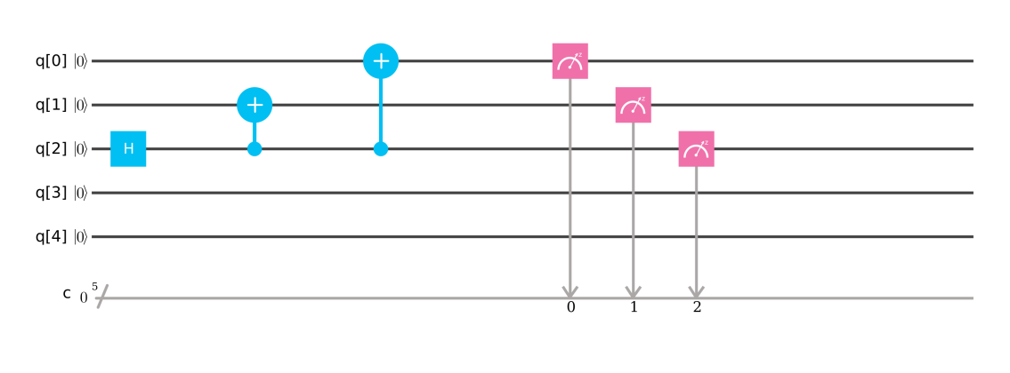
Figure 10: Circuit producing a $|\mathtt{GHZ}_{3}\rangle$ state on the IBM Q 5 Tenerife machine

The result of the experiment is in figure 11. It is interesting to note that although theoretically only the states $|00000\rangle$ and $|00111\rangle$ can be reached, the other states have a low but not zero probability of being obtained after the measure.

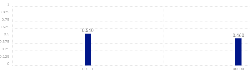
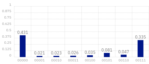
Figure 11: Execution of the circuit of figure 10. The top graphic is a simulation while the graphic on the bottom is obtained after $1024$ executions on the IBM Q 5 Tenerife machine. Both graphics have been produced through the IBM website.

Figure 12: Circuit equivalent to those of figure 10 but with more $2$-qubit gates.

Consider the circuit pictured in figure 12. Applying the results of section 4 we find that it is equivalent to those of figure 10.

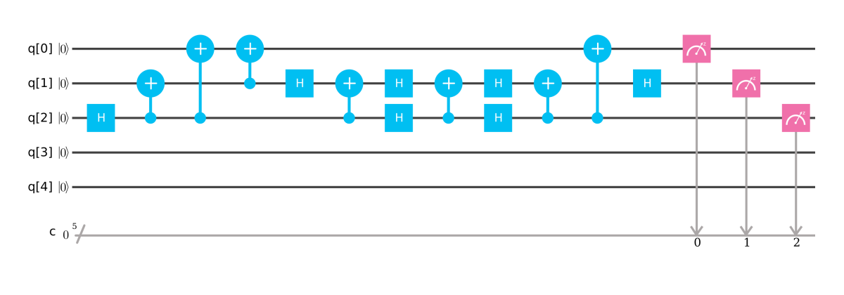
Figure 13: Circuit of 12 implemented on the IBM Q 5 Tenerife machine.

This circuit has been implemented on the IBM Q 5 Tenerife machine (see figure 13). After $1024$ executions, we observe that reliability is less good than for the circuit of figure 10. This is due to the fact that more $2$-qubit gates were used.

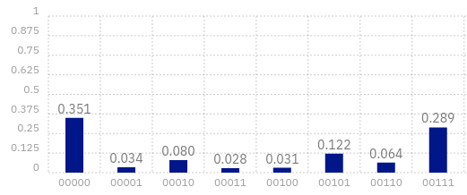
Figure 14: Execution of the circuit of figure 13. The top graphic is a simulation while the graphic on the bottom is obtained after $1024$ executions on the IBM Q 5 Tenerife machine. Both graphics have been produced through the IBM website.

Appendix B Proofs of Theorems 2 and 4

The proofs are based on two well known facts about group presentations.

Claim 13

(See eg. [35])
Let $G_{1}=\langle\mathcal{S}_{1}|\mathcal{R}_{1}\rangle$ and $G_{2}=\langle\mathcal{S}_{2}|\mathcal{R}_{2}\rangle$ be two groups given by presentation. The semidirect product $G_{1}\rtimes_{\Phi}G_{2}$ is isomorphic to

$$\langle\mathcal{S}_{1}\cup\mathcal{S}_{2}|\mathcal{R}_{1}\cup\mathcal{R}_{2}\cup\{g_{2}g_{1}g_{2}^{-1}\left(\Phi(g_{2})(g_{1})\right)^{-1}\mid g_{1}\in\mathcal{S}_{1},g_{2}\in\mathcal{S}_{2}\}\rangle.$$ (59)

Claim 14

Let $G=\langle\mathcal{S}|\mathcal{R}\rangle$. We suppose that $\mathcal{S}$ splits into two subsets $\mathcal{S}_{1}$ and $\mathcal{S}_{2}$ such that $\mathcal{S}_{2}$ is include to the subgroup of $G$ generted by $\mathcal{S}_{1}$. Let $\mathcal{R}_{1}$ denote the set of relations in $\mathcal{R}$ that involves at least an element of $\mathcal{S}_{2}$ and $\mathcal{R}_{2}=\mathcal{R}\setminus\mathcal{R}_{1}$. We construct a set $\mathcal{R}^{\prime}_{2}$ by replacing in $\mathcal{R}_{2}$ each occurrence of an element of $\mathcal{S}_{2}$ by an equivalent product of elements of $\mathcal{S}_{1}$. Obviously, one obtains that $G$ is isomorphic to $\langle G|\mathcal{R}_{1}\cup\mathcal{R}_{2}^{\prime}\rangle.$

Example 15

Let us illustrate our purpose by giving a presentation of $\mathtt{cZS}$₃. First we remark that $\mathfrak{P}_{3}$ is isomorphic to $\langle z_{0},z_{1},z_{02}|z_{0}^{2},z_{1}^{2},z_{02}^{2},(z_{0}z_{02})^{2},(z_{0}z_{1})^{2},(z_{0}z_{02})^{2}\rangle$ and $\mathfrak{S}_{3}$ is isomorhic to $\langle s_{0},s_{1}|s_{0}^{2},s_{1}^{2},(s_{0}s_{1})^{3}\rangle$. One applies Claim 13 from Theorem 1 and obtains that $\mathtt{cZS}$₃ is isomorphic to $\langle z_{0},z_{1},z_{02},s_{0},s_{1}|\mathcal{R}\rangle,$ where

$$\mathcal{R}=\{z_{0}^{2},z_{1}^{2},z_{02}^{2},(z_{0}z_{02})^{2},(z_{0}z_{1})^{2},(z_{0}z_{02})^{2},(z_{1}z_{02})^{2},s_{0}^{2},s_{1}^{2},(s_{0}s_{1})^{3},(z_{0}s_{0})^{2},(z_{1}s_{1})^{2},s_{1}z_{0}s_{1}z_{02},s_{0}z_{1}s_{0}z_{02}\}.$$

We apply Claim 14 with $\mathcal{S}_{1}=\{z_{0},z_{1},s_{0},s_{1}\}$ and $\mathcal{S}_{2}=\{z_{02}\}$. Indeed we note that $z_{02}=s_{1}z_{0}s_{1}$. Hence

$$\mathcal{R}_{1}=\{z_{0}^{2},z_{1}^{2},(z_{0}z_{1})^{2},s_{0}^{2},s_{1}^{2},(s_{0}s_{1})^{3},(z_{0}s_{0})^{2},(z_{1}s_{1})^{2}\}$$

and

$$\mathcal{R}_{2}=\{z_{02}^{2},(z_{1}z_{02})^{2},(z_{0}z_{02})^{2},s_{1}z_{0}s_{1}z_{02},s_{0}z_{1}s_{0}z_{02}\},$$

and so

$$\mathcal{R}^{\prime}_{2}=\{(s_{1}z_{0}s_{1})^{2},(z_{1}s_{1}z_{0}s_{1})^{2},(z_{0}s_{1}z_{0}s_{1})^{2},s_{1}z_{0}s_{1}s_{1}z_{0}s_{1},s_{0}z_{1}s_{0}s_{1}z_{0}s_{1}\}.$$

Since, $s_{1}^{2}=z_{0}^{2}=1$ we can remove the relation $s_{1}z_{0}s_{1}s_{1}z_{0}s_{1}$ from $\mathcal{R}^{\prime}_{2}$. Furthermore, $s_{0}z_{1}s_{0}s_{1}z_{0}s_{1}=1$ implies $(z_{1}s_{1}z_{0}s_{1})^{2}=(z_{1}s_{0})^{4}$. Hence, $\mathtt{cZS}$₃ is isomorphic to

$$\langle z_{0},z_{1},s_{0},s_{1}|z_{0}^{2},z_{1}^{2},s_{0}^{2},s_{1}^{2},(s_{0}s_{1})^{3},(z_{0}z_{1})^{2},(z_{0}s_{0})^{2},(z_{1}s_{1})^{2},(z_{0}s_{1})^{4},(z_{1}s_{0})^{4},s_{0}s_{1}z_{0}s_{1}s_{0}z_{1}\rangle.$$

Assuming that $s_{0}s_{1}z_{0}s_{1}s_{0}z_{1}=(z_{0}s_{0})^{2}=(z_{0}s_{1})^{4}=s_{0}^{2}=s_{1}^{1}=1$, one finds

$$(z_{1}s_{1})^{2}=s_{0}s_{1}(z_{0}s_{0})^{2}s_{1}s_{0}=1,$$

$$(z_{0}z_{1})^{2}=s_{0}(z_{0}s_{1})^{4}s_{0}=1,$$

$$(z_{1}s_{0})^{4}=s_{1}(z_{0}z_{1})^{2}s_{1}=1.$$

Then we simplify the presentation of $\mathtt{cZS}$₃ as

$$\langle z_{0},z_{1},s_{0},s_{1}|z_{0}^{2},z_{1}^{2},s_{0}^{2},s_{1}^{2},(s_{0}s_{1})^{3},(z_{0}s_{0})^{2},(z_{0}s_{1})^{4},s_{0}s_{1}z_{0}s_{1}s_{0}z_{1}\rangle.$$

Reformulated in terms of presentation Theorem 2 reads:

Theorem 16

Suppose $k\geq 2$. The group $\mathtt{cZS}$_k is isomorphic to the presentation $\langle z_{0},\dots,z_{k-2},s_{0},\dots,s_{k-2}|\mathcal{R}\rangle$ where $\mathcal{R}$ is the following set of relations

1. for any $0\leq i\leq k-2$, $z_{i}^{2}=s_{i}^{2}=1$,

2. for any $0\leq i<j\leq k-2$ such that $j-i>1$, $(s_{i}s_{j})^{2}=1$,

3. for any $0\leq i\leq k-3$, $(s_{i}s_{i+1})^{3}=1$,

4. for any $0\leq i<j\leq k-2$, $(z_{i}z_{j})^{2}=1$,

5. for any $0\leq i,j\leq k-2$ such that $|i-j|\neq 1$, $(z_{i}s_{j})^{2}=1$,

6. for any $0\leq i,j\leq k-2$ such that $|i-j|=1$, $(z_{i}s_{j})^{4}=1$,

7. for any $0\leq i\leq k-3$, $s_{i}s_{i+1}z_{i}s_{i+1}s_{i}z_{i+1}=1$.

Proof If $k=2$ the result is straightforward from the definition. Now we assume $k\geq 3$. We apply Claim 13 and find a presentation of $\mathtt{cZS}$_k as $\langle\mathcal{S}|\mathcal{R}\rangle$ with

$$\mathcal{S}=\mathcal{T}\cup\mathcal{Z}$$

and

$$\mathcal{R}=\mathcal{RS}\cup\mathcal{RZ}\cup\mathcal{RC},$$

where $\mathcal{T}=\{s_{i}\mid 0\leq i\leq k-2\}$, $\mathcal{Z}=\{z_{\{i,j\}}\mid 0\leq i\leq j-1\leq k-2\}$, $\mathcal{RS}=\{s_{i}^{2}\mid 0\leq i\leq k-3\}\cup\{(s_{i}s_{j})^{2}\mid 0\leq i<j-1\leq k-3\}\cup\{(s_{i}s_{i+1})^{3}\mid 0\leq i\leq k-3\}$, $\mathcal{RZ}=\{z_{\{i,j\}}^{2}\mid 0\leq i<j\leq k-1\}\cup\{(z_{\{i,j\}}z_{\{p,q\}})^{2}\mid 0\leq i\leq j-1\leq k-2,0\leq p\leq q-1\leq k-2\}$, and $\mathcal{RC}=\{s_{p}z_{\{i,j\}}s_{p}z_{\{s_{p}(i),s_{p}(j)\}}|0\leq i<j\leq k-1,0\leq p\leq k-2\}.$The set $\mathcal{RS}$ means that the subgroup $G_{S}=\langle T|\mathcal{RS}\rangle$ is isomorphic to the symmetric group $\mathfrak{S}_{k}$. The set $\mathcal{RZ}$ means that the subgroup $G_{Z}=\langle\mathcal{Z}|\mathcal{RZ}\rangle$ is isomorphic to $\mathbb{Z}_{2}^{\left(k\atop 2\right)}$. The set $\mathcal{R}C$ encodes the conjugacy of an element of $\mathcal{Z}$ by an element of $G_{S}$. More precisely, if $\sigma$ is a permutation of $\mathfrak{S}_{k}$ and $w_{\sigma}$ denotes the image of $\sigma$ in $G_{S}$ then the relations of $\mathcal{R}S$ and $\mathcal{R}C$ implies

$$w_{\sigma}z_{\{i,j\}}w_{\sigma}^{-1}=z_{\{\sigma(i),\sigma(j)\}}.$$ (60)

For simplicity, in the rest of the proof we set $z_{ij}:=z_{\{i,j\}}$ and $z_{i}:=z_{ii+1}$. The relation $z_{ij}^{2}=1$ can be recovered from $z_{i}^{2}=1$ and the relations of $\mathcal{RS}\cup\mathcal{RC}$. Indeed it suffices to consider a permutation $\sigma$ sending $\{i,j\}$ to $\{i,i+1\}$ and write $z_{ij}^{2}=(w_{\sigma}^{-1}z_{i}w_{\sigma})^{2}=w_{\sigma}^{-1}z_{i}^{2}w_{\sigma}=1$. In the same way, if $\sigma$ is a permutation sending $\{i,j\}$ to $\{i_{1},i_{1}+1\}$ and $\{p,q\}$ to $\{i_{2},i_{2}+1\}$ for some $0\leq i<j\leq k-1$, $0\leq p<q\leq k-1$, $i\neq p$, $j\neq q$ and $0\leq i_{1},i_{2}\leq k-2$ we have $(z_{ij}z_{pq})^{2}=(w_{\sigma}^{-1}z_{i_{1}}w_{\sigma}w_{\sigma}^{-1}z_{i_{2}}w_{\sigma})^{2}=w_{\sigma}^{-1}(z_{i_{1}}z_{i_{2}})^{2}w_{\sigma}$. So the relation $(z_{ij}z_{pq})^{2}=1$ can be recovered from $(z_{i_{1}}z_{i_{2}})^{2}=1$ and the relations of $\mathcal{RS}\cup\mathcal{RC}$. If ($i=p$ and $j\neq q$) or ($i\neq p$ and $j=q$), there exists no permutation sending $\{i,j\}$ to $\{i_{1},i_{1}+1\}$ and $\{p,q\}$ to $\{i_{2},i_{2}+1\}$ for some $0\leq i_{1},i_{2}\leq k-2$. We introduce the set of relations $\mathcal{RSZ}:=\{(z_{i}s_{j})^{4}|0\leq i,j\leq k-2,|i-j|=1\}$. These relations can be recovered from $\mathcal{R}$ since $(z_{i}s_{i+1})^{4}=(z_{i}z_{ii+2})^{2}$ and $(z_{i}s_{i-1})^{4}=(z_{i}z_{i-1i+1})^{2}$. If ($i=p$ and $j\neq q$) or ($i\neq p$ and $j=q$) then there exists a permutation $\sigma$ sending $\{i,j\}$ to $\{i_{1},i_{1}+1\}$ and $\{p,q\}$ to $\{i_{1},i_{1}+2\}$ for some $0\leq i_{1}\leq k-3$. Hence, $(z_{ij}z_{pq})^{2}=(w_{\sigma}^{-1}z_{i_{1}}z_{i_{1}i_{1}+2}w_{\sigma})^{2}=w_{\sigma}^{-1}(z_{i_{1}}z_{i_{1}i_{1}+2})^{2}w_{\sigma}=w_{\sigma}^{-1}(z_{i_{1}}s_{i_{1}+1})^{4}w_{\sigma}$.
As a conclusion, we deduce that $\langle\mathcal{S}|\mathcal{R}\rangle=\langle\mathcal{S}|\mathcal{R}^{\prime}\rangle$ with $\mathcal{R}^{\prime}=\mathcal{RS}\cup\mathcal{RZ^{\prime}}\cup\mathcal{RC}\cup\mathcal{RSZ}$ and $\mathcal{RZ}^{\prime}=\{z_{i}^{2}\mid 0\leq i\leq k-2\}\cup\{(z_{i}z_{p})^{2}\mid 0\leq i,p\leq k-2\}$.
Now let us remove redundancies in $\mathcal{RC}$ and proves that it can be replaced by $\mathcal{RC^{\prime}}:=\{(s_{j}z_{i})^{2}\mid|i-j|\neq 1\}\cup\{s_{i}s_{i+1}z_{i}s_{i+1}s_{i}z_{i+1}\mid 0\leq i\leq k-3\}\cup\{s_{j-1}z_{ij}s_{j-1}z_{ij-1}\mid 0\leq i\leq j-2\leq k-3\}$ in the presentation. The first and the last sets of the definition of $\mathcal{RC}^{\prime}$ are include in $\mathcal{RC}$. Furthermore, in $\langle\mathcal{S}|\mathcal{R}^{\prime}\rangle$, we have $s_{i}s_{i+1}z_{i}s_{i+1}s_{i}z_{i+1}=s_{i}z_{ii+2}s_{i}z_{i+1}\in\mathcal{RC}$. Conversely, we set $\mathcal{R^{\prime\prime}}:=\mathcal{RS}\cup\mathcal{RZ^{\prime}}\cup\mathcal{RC^{\prime}}\cup\mathcal{RSZ}$ and we prove that for any $w\in\mathcal{RC}$, we have $w=1$ in $\langle S|\mathcal{R}^{\prime\prime}\rangle$. Indeed, we have $\mathcal{RC}\setminus\mathcal{RC^{\prime}}\subset\{s_{p}z_{ij}s_{p}z_{ij}|p\not\in\{i-1,i,j-1,j\}\cup\{s_{j}z_{ij}s_{j}z_{ij+1}\mid 0\leq i\leq j-1\leq k-3\}\cup\{s_{i-1}z_{ij}s_{i-1}z_{i-1j}\mid 1\leq i<j\leq k-1\}\cup\{s_{i}z_{ij}s_{i}z_{i+1j}\mid 0\leq i\leq j-2\leq k-3\}.$ So we have to consider $4$ cases:

1. Consider the element $s_{j}z_{ij}s_{j}z_{ij+1}$ with $0\leq i\leq j-1\leq k-3$. We have $s_{j}z_{ij}s_{j}z_{ij+1}=(z_{ij+1}s_{j}z_{ij}s_{j})^{-1}=s_{j}(s_{j}z_{ij+1}s_{j}z_{ij})^{-1}s_{j}=s_{j}^{2}=1$ in $\langle\mathcal{S}\mid\mathcal{R}^{\prime\prime}\rangle$.

2. Consider the element $s_{i-1}z_{ij}s_{i-1}z_{i-1j}$ with $1\leq i<j\leq k-1$. If $i=j-1$ then, using the second and third sets of the definition of $\mathcal{RC^{\prime}}$ one obtains $s_{i-1}z_{ii+1}s_{i-1}z_{i-1i+1}=s_{i-1}z_{i}s_{i-1}s_{i}z_{i-1}s_{i}=s_{i-1}z_{i}z_{i}s_{i-1}=1$ in $\langle\mathcal{S}\mid\mathcal{R}^{\prime\prime}\rangle$. If $i<j-1$ then $s_{i-1}z_{ij}s_{i-1}z_{i-1j}=s_{i-1}s_{j-1}z_{ij-1}s_{j-1}s_{i-1}s_{j-1}z_{i-1j-1}s_{j-1}=s_{j-1}s_{i-1}z_{ij-1}s_{i-1}z_{i-1j-1}s_{j-1}$ and, using an induction on $|i-j|$ one finds $s_{j-1}s_{i-1}z_{ij-1}s_{i-1}z_{i-1j-1}s_{j-1}=s_{j-1}^{2}=1$ in $\langle\mathcal{S}\mid\mathcal{R}^{\prime\prime}\rangle$.

3. Consider the element $s_{i}z_{ij}s_{i}z_{i+1j}$ for $0\leq i<j-2\leq k-3$. We have $s_{i}z_{ij}s_{i}z_{i+1j}=s_{i}(s_{i}z_{i+1j}s_{i}z_{ij})^{-1}s_{i}=1$ from the previous case.

4. Suppose $p\not\in\{i-1,i,j-1,j\}$. We proceed by induction on $|i-j|$. If $j=i+1$ then the result is directly obtains from the first set of the definition of $\mathcal{RC}^{\prime}$. If $p=i+1=j-2$ then we use the previous cases and obtains $s_{i+1}z_{ii+3}s_{i+1}z_{ii+3}=s_{i+1}s_{i+2}s_{i+1}z_{i}s_{i+1}s_{i+2}s_{i+1}s_{i+2}s_{i+1}z_{i}s_{i+1}s_{i+2}.$ Hence using the fact that $z_{i}$ and $s_{i+2}$ commute in $\langle\mathcal{S}\mid\mathcal{R}^{\prime\prime}\rangle$ together with the braid relations, one obtains $s_{i+1}s_{i+2}s_{i+1}z_{i}s_{i+1}s_{i+2}s_{i+1}s_{i+2}s_{i+1}z_{i}s_{i+1}s_{i+2}=s_{i+2}s_{i+1}s_{i+2}z_{i}s_{i+2}z_{i}s_{i+1}s_{i+2}=1.$

   If $p\neq j-2$ then $s_{p}z_{ij}s_{p}z_{ij}=s_{p}s_{j-1}z_{ij-1}s_{j-1}s_{p}s_{j-1}z_{ij-1}s_{j-1}=s_{j-1}s_{p}z_{ij-1}s_{p}z_{ij-1}s_{j-1}=1$ using the induction hypothesis. Finally, if $p\neq i+1$ then $s_{p}z_{ij}s_{p}z_{ij}=s_{p}s_{i}z_{i+1j}s_{i}s_{p}s_{i}z_{i+1j}s_{i}=s_{i}s_{p}z_{i+1j}s_{p}z_{i+1j}s_{i}=1$ using the induction hypothesis.

So we have proved that $\langle S\mid\mathcal{R}\rangle=\langle S\mid\mathcal{R}^{\prime\prime}\rangle$. Now we apply Claim 14 with $\mathcal{S}_{1}=\{z_{i}\mid 0\leq i\leq k-2\}\cup\{s_{i}\mid 0\leq i\leq k-2\}$ and $\mathcal{S}_{2}=\{z_{ij}\mid 0\leq i\leq j-2\leq k-3\}$. We obtain $\mathcal{R}^{\prime\prime}=\mathcal{R}_{1}\cup\mathcal{R}_{2}$ with $\mathcal{R}_{1}=\mathcal{RS}\cup\mathcal{RZ^{\prime}}\cup\mathcal{RSZ}\cup\{(z_{i}s_{j})^{2}\mid|i-j|\neq 1\}\cup\{s_{i}s_{i+1}z_{i}s_{i+1}s_{i}z_{i+1}\mid 0\leq i\leq k-3\}$ and $\mathcal{R}_{2}=\{s_{j-1}z_{ij}s_{j-1}z_{ij-1}\mid 0\leq i\leq j-2\leq k-3\}$. To obtain $\mathcal{R}^{\prime}_{2}$, we substitute each occurrence of $z_{ij}$ in $\mathcal{R}_{2}$ by $s_{j-1}s_{j-2}\cdots s_{i+1}z_{i}s_{i+1}\cdots s_{j-2}s_{j-1}$. In other words,

$$\mathcal{R}^{\prime}_{2}=\{s_{j-1}\cdot s_{j-1}s_{j-2}\cdots s_{i+1}z_{i}s_{i+1}\cdots s_{j-1}\cdot s_{j-1}\cdot{}s_{j-2}\cdots s_{i+1}z_{i}s_{i+1}\cdots s_{j-2}\mid 0\leq i\leq j-2\leq k-3\}.$$

But each $s_{j-1}\cdot s_{j-1}s_{j-2}\cdots s_{i+1}z_{i}s_{i+1}\cdots s_{j-1}\cdot s_{j-1}\cdot{}s_{j-2}\cdots s_{i+1}z_{i}s_{i+1}\cdots s_{j-2}$ reduces to $1$ by using rules of $\mathcal{RS}$ and $\mathcal{RZ}^{\prime}$. Hence we deduce that $\langle\mathcal{S}|\mathcal{R}\rangle=\langle\mathcal{S}_{1}|\mathcal{R}_{1}\rangle$, as expected. $\Box$

Theorem 4 is restated as

Theorem 17

For $k\geq 2$, the group $\mathtt{cZS}$_k is isomorphic to the group $\langle g_{0},g_{1},g_{2},\dots,g_{k-1}|\mathcal{R}_{k}\rangle$, where $\mathcal{R}_{k}$ is the set of the following relations:

1. For any $0\leq i\leq k-1$, $g_{i}^{2}=1$,

2. For any $1\leq i<j\leq k-1$ such that $|i-j|>1$, $(g_{i}g_{j})^{2}=1$,

3. For any $1\leq i\leq k-2$, $(g_{i}g_{i+1})^{3}=1$,

4. For any $i=1,3,\dots k-1$, $(g_{0}g_{i})^{2}=1$,

5. $(g_{0}g_{2})^{4}=1$,

6. $(g_{0}g_{2}g_{3}g_{1}g_{2})^{4}=1$.

The explicit isomorphism sends $Z_{0}$ to $g_{0}$ and each $S_{i}$ to $g_{i+1}$.

Proof We find several redundancies in the presentation of Theorem 16. First we compute

$$\begin{array}[]{rcl}(z_{i}s_{i-1})^{4}&\displaystyle\mathop{=}^{(vii),(i)}&(s_{i-1}s_{i}z_{i-1}s_{i})^{4}\\ &\displaystyle\mathop{=}^{(iii),(v)}&(s_{i-1}s_{i}z_{i-1}s_{i-1}s_{i}z_{i-1}s_{i-1}s_{i})^{2}\\ &\displaystyle\mathop{=}^{(iii),(i)}&s_{i}s_{i-1}(s_{i}z_{i-1})^{4}s_{i-1}s_{i}.\end{array}$$ (61)

The overscripted numbers correspond to the rules of Theorem 16 used to obtain each equality. Assuming $(z_{i-1}s_{i})^{4}=1$ and applying the rule $(i)$, we show that $(z_{i}s_{i-1})^{4}=1$. So this relation can be removed from the presentation.
Now let us consider the relations $\{(z_{i}z_{j})^{2}=1\mid 0\leq i<j\leq k-2\}$ of point $(iv)$ of Theorem 16. If $j=i+1$ we have :

$$\begin{array}[]{rcl}(z_{i}z_{i+1})^{2}&\displaystyle\mathop{=}^{(vii)}&(z_{i}s_{i}s_{i+1}z_{i}s_{i+1}s_{i})^{2}\\ &\displaystyle\mathop{=}^{(v)}&(s_{i}z_{i}s_{i+1}z_{i}s_{i+1}s_{i})^{2}\\ &\displaystyle\mathop{=}^{(i)}&s_{i}(z_{i}s_{i+1})^{4}s_{i}.\end{array}$$

Assuming $(z_{i}s_{i+1})^{4}=1$ and applying the rule $(i)$ we have $(z_{i}z_{i+1})^{2}=1$ so this relation can also be removed from the presentation.

If $j=i+2$ then we have

$$\begin{array}[]{rcl}(z_{i}z_{i+2})^{2}&\displaystyle\mathop{=}^{(vii)}&(s_{i-1}s_{i}z_{i-1}s_{i}s_{i-1}z_{i+2})^{2}\\ &\displaystyle\mathop{=}^{(v)}&(s_{i-1}s_{i}z_{i-1}z_{i+2}s_{i}s_{i-1})^{2}\\ &\displaystyle\mathop{=}^{(i)}&s_{i-1}s_{i}(z_{i-1}z_{i+2})^{2}s_{i}s_{i-1}\\ &\displaystyle\mathop{=}^{(vii)}&s_{i-1}s_{i}(z_{i-1}s_{i+1}s_{i+2}z_{i+1}s_{i+2}s_{i+1})^{2}s_{i}s_{i-1}\\ &\displaystyle\mathop{=}^{(v)}&s_{i-1}s_{i}(s_{i+1}s_{i+2}z_{i-1}z_{i+1}s_{i+2}s_{i+1})^{2}s_{i}s_{i-1}\\ &\displaystyle\mathop{=}^{(i)}&s_{i-1}s_{i}s_{i+1}s_{i+2}(z_{i-1}z_{i+1})^{2}s_{i+2}s_{i+1}s_{i}s_{i-1}.\end{array}$$

Hence by induction on $i$, assuming that $(z_{0}z_{2})^{2}=1$, we show that $(z_{i}z_{i+2})^{2}=1$.

If $j>i+2$, then we have

$$\begin{array}[]{rcl}(z_{i}z_{j})^{2}&\displaystyle\mathop{=}^{(vii)}&(z_{i}s_{j-1}s_{j}z_{j-1}s_{j}s_{j-1})^{2}\\ &\displaystyle\mathop{=}^{(v)}&(s_{j-1}s_{j}z_{i}z_{j-1}s_{j}s_{j-1})^{2}\\ &\displaystyle\mathop{=}^{(i)}&s_{j-1}s_{j}(z_{i}z_{j-1})^{2}s_{j}s_{j-1}\\ \end{array}.$$

Hence by induction on $j$, assuming that $(z_{i}z_{i+2})^{2}=1$, we show that $(z_{i}z_{j})^{2}=1$.

To summarize we have shown that, assuming points $(vii),(vi),(v),(i)$ of Theorem 16, all the relations of point $(iv)$ (i.e $\{(z_{i}z_{j})^{2}=1\mid 0\leq i<j\leq k-2\}$) are redundancies except one : $(z_{0}z_{2})^{2}=1$. We also notice that $(z_{0}z_{2})^{2}=(z_{0}s_{1}s_{2}s_{0}s_{1}z_{0}s_{1}s_{0}s_{2}s_{1})^{2}=(z_{0}s_{1}s_{2}s_{0}s_{1})^{4}$

Now we apply Claim 14 by setting $\mathcal{S}_{1}=\{z_{0},s_{0},\dots,s_{k-2}\}$ and $\mathcal{S}_{2}=\{z_{1},\dots,z_{k-2}\}$ since

$$z_{i}=(s_{i-1}s_{i})\cdots(s_{0}s_{1})z_{0}(s_{1}s_{0})\cdots(s_{i}s_{i-1}).$$ (62)

We have

$$\mathcal{R}_{1}=\mathcal{RS}\cup\{z_{0}^{2}=1,(z_{0}s_{1})^{4}=1,(z_{0}s_{1}s_{2}s_{0}s_{1})^{4}=1\}\cup\{(z_{0}s_{j})^{2}=1\mid j\neq 1\}$$

and

$$\begin{array}[]{rcl}\mathcal{R}_{2}&=&\{z_{i}^{2}=1\mid 1\leq i\leq k-2\}\cup\{(z_{i}s_{i+1})^{4}=1\mid 1\leq i\leq k-3\}\\ &&\cup\{(z_{i}s_{j})^{2}=1\mid 1\leq i,j\leq k-2,j\not\in\{i-1,i+1\}\\ &&\cup\{s_{i}s_{i+1}z_{i}s_{i+1}s_{i}z_{i+1}=1\mid 0\leq i\leq k-3\}\\ \end{array}$$

So we have $\mathcal{R}^{\prime}_{2}=\mathcal{T}_{1}\cup\mathcal{T}_{2}\cup\mathcal{T}_{3}\cup\mathcal{T}_{4}$ with

$$\mathcal{T}_{1}=\{((s_{i-1}s_{i})\cdots(s_{0}s_{1})z_{0}(s_{1}s_{0})\cdots(s_{i}s_{i-1}))^{2}=1\mid 1\leq i\leq k-2\}$$

$$\mathcal{T}_{2}=\{((s_{i-1}s_{i})\cdots(s_{0}s_{1})z_{0}(s_{1}s_{0})\cdots(s_{i}s_{i-1})s_{i+1})^{4}=1\mid 1\leq i\leq k-3\}$$

$$\mathcal{T}_{3}=\{((s_{i-1}s_{i})\cdots(s_{0}s_{1})z_{0}(s_{1}s_{0})\cdots(s_{i}s_{i-1})s_{j})^{2}=1\mid 1\leq i,j\leq k-2,j\not\in\{i-1,i+1\}$$

$$\begin{array}[]{l}\mathcal{T}_{4}=\{s_{i}s_{i+1}(s_{i-1}s_{i})\cdots(s_{0}s_{1})z_{0}(s_{1}s_{0})\cdots(s_{i}s_{i-1})s_{i+1}s_{i}(s_{i}s_{i+1})\cdots(s_{0}s_{1})z_{0}(s_{1}s_{0})\cdots(s_{i+1}s_{i})=1\\ \mid 0\leq i\leq k-3\}.\end{array}$$

Remarking that $\displaystyle((s_{i-1}s_{i})\cdots(s_{0}s_{1})z_{0}(s_{1}s_{0})\cdots(s_{i}s_{i-1}))^{2}\mathop{=}^{\mathcal{R}_{1}}1$ we can remove the relation of $\mathcal{T}_{1}$ from $\mathcal{R}^{\prime}_{2}$.

In order to remove the relations of $\mathcal{T}_{3}$ from $\mathcal{R}^{\prime}_{2}$ we distinguish three cases :

1. If $j>i+1$ then

   $$\begin{array}[]{rcl}\displaystyle((s_{i-1}s_{i})\cdots(s_{0}s_{1})z_{0}(s_{1}s_{0})\cdots(s_{i}s_{i-1})s_{j})^{2}&\displaystyle\mathop{=}^{\mathcal{R}_{1}}&((s_{i-1}s_{i})\cdots(s_{0}s_{1})z_{0}(s_{1}s_{0})\cdots(s_{i}s_{i-1}))^{2}s_{j}^{2}\\ &\displaystyle\mathop{=}^{\mathcal{R}_{1}}&1.\end{array}$$

2. If $j=i$ then we use the the braid relations and obtain

   $$(s_{1}s_{0})\cdots(s_{i}s_{i-1})s_{i}\mathop{=}^{braid}s_{0}(s_{1}s_{0})\cdots(s_{i}s_{i-1}).$$ (63)

   Hence,

   $$\begin{array}[]{rcl}\displaystyle((s_{i-1}s_{i})\cdots(s_{0}s_{1})z_{0}(s_{1}s_{0})\cdots(s_{i}s_{i-1})s_{i})^{2}&\displaystyle\mathop{=}^{braid}&((s_{i-1}s_{i})\cdots(s_{0}s_{1})z_{0}s_{0}(s_{1}s_{0})\cdots(s_{i}s_{i-1}))^{2}\\ &\displaystyle\mathop{=}^{\mathcal{R}_{1}}&(s_{i-1}s_{i})\cdots(s_{0}s_{1})(z_{0}s_{0})^{2}(s_{1}s_{0})\cdots(s_{i}s_{i-1})\\ &\displaystyle\mathop{=}^{\mathcal{R}_{1}}&1.\end{array}$$

3. If $j<i-1$ then we have

   $$\begin{array}[]{rcl}\displaystyle((s_{i-1}s_{i})\cdots(s_{0}s_{1})z_{0}(s_{1}s_{0})\cdots(s_{i}s_{i-1})s_{j})^{2}&\displaystyle\mathop{=}^{\mathcal{R}_{1}}&((s_{i-1}s_{i})\cdots(s_{j}s_{j+1})(s_{j-1}s_{j})\cdots(s_{0}s_{1})z_{0}\\ &&\cdot(s_{1}s_{0})\cdots(s_{j}s_{j-1})(s_{j+1}s_{j})(s_{j+2}s_{j+1})s_{j}\cdots(s_{i}s_{i-1}))^{2}\\ &\displaystyle\mathop{=}^{\mathcal{R}_{1}}&((s_{i-1}s_{i})\cdots(s_{j}s_{j+1})(s_{j-1}s_{j})\cdots(s_{0}s_{1})z_{0}\\ &&\cdot(s_{1}s_{0})\cdots(s_{j}s_{j-1})(s_{j+1}s_{j+2})(s_{j}s_{j+1}s_{j})\cdots(s_{i}s_{i-1}))^{2}\\ &\displaystyle\mathop{=}^{\mathcal{R}_{1}}&((s_{i-1}s_{i})\cdots(s_{j}s_{j+1})(s_{j-1}s_{j})\cdots(s_{0}s_{1})z_{0}\\ &&\cdot(s_{1}s_{0})\cdots(s_{j}s_{j-1})(s_{j+1}s_{j+2})(s_{j+1}s_{j}s_{j+1})\cdots(s_{i}s_{i-1}))^{2}\\ &\displaystyle\mathop{=}^{\mathcal{R}_{1}}&((s_{i-1}s_{i})\cdots(s_{j}s_{j+1})(s_{j-1}s_{j})\cdots(s_{0}s_{1})z_{0}\\ &&\cdot(s_{1}s_{0})\cdots(s_{j}s_{j-1})s_{j+2}(s_{j+1}s_{j})(s_{j+2}s_{j+1})\cdots(s_{i}s_{i-1}))^{2}\\ &\displaystyle\mathop{=}^{\mathcal{R}_{1}}&(s_{i-1}s_{i})\cdots(s_{j}s_{j+1})((s_{j-1}s_{j})\cdots(s_{0}s_{1})z_{0}\\ &&\cdot(s_{1}s_{0})\cdots(s_{j}s_{j-1})s_{j+2})^{2}(s_{j+1}s_{j})(s_{j+2}s_{j+1})\cdots(s_{i}s_{i-1})\\ &\displaystyle\mathop{=}^{\mathcal{R}_{1}}&1\ \textrm{(using the first case)}\end{array}$$

So we can remove the relations of $\mathcal{T}_{3}$ from $\mathcal{R}^{\prime}_{2}$.
Also, using the relation of the symmetric group, one finds

$$(s_{1}s_{0})\cdots(s_{i}s_{i-1})s_{i+1}(s_{i-1}s_{i})\cdots(s_{0}s_{1})\mathop{=}^{\mathcal{R}_{1}}s_{i+1}s_{i}\cdots s_{2}s_{1}s_{2}\cdots s_{i}s_{i+1}.$$ (64)

Hence,

$$\begin{array}[]{rcl}((s_{i-1}s_{i})\cdots(s_{0}s_{1})z_{0}(s_{1}s_{0})\cdots(s_{i}s_{i-1})s_{i+1})^{4}&\displaystyle\mathop{=}^{\mathcal{R}_{1}}&(s_{i-1}s_{i})\cdots(s_{0}s_{1})\\ &&\cdot(z_{0}s_{i+1}s_{i}\cdots s_{2}s_{1}s_{2}\cdots s_{i}s_{i+1})^{3}\\ &&\cdot z_{0}(s_{1}s_{0})\cdots(s_{i}s_{i-1})s_{i+1}\\ &\displaystyle\mathop{=}^{\mathcal{R}_{1}}&(s_{i-1}s_{i})\cdots(s_{0}s_{1})s_{i+1}s_{i}\cdots s_{2}\\ &&\cdot(z_{0}s_{1})^{3}z_{0}s_{2}\cdots s_{i}s_{i+1}(s_{1}s_{0})\cdots(s_{i}s_{i-1})s_{i+1}\\ &\displaystyle\mathop{=}^{\mathcal{R}_{1}}&(s_{i-1}s_{i})\cdots(s_{0}s_{1})s_{i+1}s_{i}\cdots s_{2}\\ &&\cdot(z_{0}s_{1})^{4}s_{2}\cdots s_{i}s_{i+1}(s_{1}s_{0})\cdots(s_{i}s_{i-1})\\ &\displaystyle\mathop{=}^{\mathcal{R}_{1}}&1.\end{array}$$

We deduce that we can remove the relation of $\mathcal{T}_{2}$. Finally the relation $s_{i}s_{i+1}(s_{i-1}s_{i})\cdots(s_{0}s_{1})z_{0}(s_{1}s_{0})\cdots(s_{i}s_{i-1})s_{i+1}s_{i}(s_{i}s_{i+1})\cdots(s_{0}s_{1})z_{0}(s_{1}s_{0})\cdots(s_{i+1}s_{i})$ reduces to $1$ using only $s_{i}^{2}=z_{0}^{2}=1$. The relations of $\mathcal{T}_{4}$ are redundancies. Hence, the group $\mathtt{cZS}$_k is isomorphic to $\langle\mathcal{S}_{1}|\mathcal{R}_{1}\rangle$ and we recover the statement of Theorem 17 by sending $z_{0}$ to $g_{0}$ and each $s_{i}$ to $g_{i+1}$. $\Box$

Appendix C Entanglement of $|\mathtt{GHZ}_{k}\rangle$

In this section, we prove that the state $|\mathtt{GHZ}_{k}\rangle$ is not generically entangled. We start with a result of Miyake [25] stating that a state is generically entangled if and only if its hyperdeterminant $\Delta$ does not vanish. The hyperdeterminant is a high degree invariant polynomial impossible to compute in practice but its interpretation in terms of solutions to a system of equations allows us to test its nullity, see e.g. [33] p445. Let us recall briefly how to process. First we consider $k$ binary variables $\mathbf{x}^{(i)}=(x^{(i)}_{0},x^{(i)}_{1})$, $i=1..k$. To each state $|\phi\rangle=\sum\alpha_{i_{1}\dots i_{k}}|i_{1}\cdots i_{k}\rangle$, we associate the binary multilinear form

$$f_{\phi}:=\sum_{0\leq i_{1},\dots,i_{k}\leq 1}\alpha_{i_{1},\dots,i_{k}}x_{i_{1}}^{(1)}\cdots x_{i_{k}}^{(k)}.$$ (65)

The hyperdeterminant vanishes if and only if the system

$$\{f_{\phi}=0\}\cup\{{d\over dx^{(j)}_{i}}f_{\phi}=0\mid 0\leq i\leq 1,1\leq j\leq k\}$$ (66)

has a non trivial solution $\hat{\mathbf{x}}^{(1)},\dots,\hat{\mathbf{x}}^{(k)}$, ie such that there exists $1\leq j\leq k$ with $\hat{\mathbf{x}}^{(j)}\neq(0,0)$. For $|\mathtt{GHZ}_{k}\rangle$ the system is

$$\begin{array}[]{l}x_{0}^{(1)}\cdots x_{0}^{(k)}+x_{1}^{(1)}\cdots x_{1}^{(k)}=x_{0}^{(2)}\cdots x_{0}^{(k)}=x_{1}^{(2)}\cdots x_{1}^{(k)}=x_{0}^{(1)}x_{0}^{(3)}\cdots x_{0}^{(k)}\\ =x_{1}^{(1)}x_{1}^{(3)}\cdots x_{1}^{(k)}=\cdots=x_{0}^{(1)}\cdots x_{0}^{(k-1)}=x_{1}^{(1)}\cdots x_{1}^{(k-1)}=0.\end{array}$$ (67)

We check that for $k>3$, $x_{0}^{(1)}=x_{0}^{(2)}=x_{1}^{(3)}=x_{1}^{(4)}=0$ implies (67). So for $k>3$, $|\mathtt{GHZ}_{k}\rangle$ is not generically entangled. Remark that, when $k=2,3$, all the solutions of (67) are trivial and so $|\mathtt{GHZ}_{k}\rangle$ is generically entangled.

Appendix D Some covariant polynomials associated to $4$ qubit systems

In this section, we shall explain how to compute the polynomials which are used to determine the entanglement type of the systems in section 5.3.We shall first recall the definition of the transvection of two multi-binary forms on the binary variables $x^{(1)}=(x^{(1)}_{0},x^{(1)}_{1}),\dots,x^{(p)}=(x^{(p)}_{0},x^{(p)}_{1})$

$$(f,g)_{i_{1},\dots,i_{p}}={\mathrm{t}r}\Omega^{i_{1}}_{x^{(1)}}\dots\Omega_{x^{(p)}}^{i_{p}}f(x^{\prime(1)},\dots,x^{\prime(p)})g(x^{\prime\prime(1)},\dots,x^{\prime\prime(p)}),$$ (68)

where $\Omega$ is the Cayley operator

$$\Omega_{x}=\left|\begin{array}[]{cc}\partial\over\partial x^{\prime}_{0}&\partial\over\partial x^{\prime\prime}_{0}\\ \partial x^{\prime}_{1}&\partial\over\partial x^{\prime\prime}_{1}\end{array}\right|$$

and $\rm tr$ sends each variables $x^{\prime},x^{\prime\prime}$ on $x$ (erases ^′ and ^′′). In [27], we give a list of generators of the algebra of covariant polynomials for $4$ qubits systems which are obtained by transvection from the ground form

$${}A=\sum_{i,j,k,\ell}\alpha_{i,j,k,l}x_{i}y_{j}z_{k}t_{\ell}.$$

Here we give formulas for some of the polynomials which are used in the paper. $\begin{array}[]{cc}&\\ \begin{array}[]{|c|c|}\hline\cr\mbox{Symbol}&\mbox{Transvectant}\\ \hline\cr B_{2200}&\frac{1}{2}(A,A)^{0011}\\ B_{2020}&\frac{1}{2}(A,A)^{0101}\\ B_{2002}&\frac{1}{2}(A,A)^{0110}\\ B_{0220}&\frac{1}{2}(A,A)^{1001}\\ B_{0202}&\frac{1}{2}(A,A)^{1010}\\ B_{0022}&\frac{1}{2}(A,A)^{1100}\\ \hline\cr\end{array}&\begin{array}[]{|c|c|}\hline\cr\mbox{Symbol}&\mbox{Transvectant}\\ \hline\cr C^{1}_{1111}&(A,B_{2200})^{1100}+(A,B_{0022})^{0011}\\ \hline\cr C_{3111}&\frac{1}{3}\left((A,B_{2200})^{0100}+(A,B_{2020})^{0010}+(A,B_{2002})^{0001}\right)\\ C_{1311}&\frac{1}{3}\left((A,B_{2200})^{1000}+(A,B_{0220})^{0010}+(A,B_{0202})^{0001}\right)\\ C_{1131}&\frac{1}{3}\left((A,B_{2020})^{1000}+(A,B_{0220})^{0100}+(A,B_{0022})^{0001}\right)\\ C_{1113}&\frac{1}{3}\left((A,B_{2002})^{1000}+(A,B_{0202})^{0100}+(A,B_{0022})^{0010}\right)\\ \hline\cr\end{array}\end{array}$

$\begin{array}[]{cc}\begin{array}[]{c}\begin{array}[]{|c|c|}\hline\cr\mbox{Symbol}&\mbox{Transvectant}\\ \hline\cr D_{2200}&(A,C_{1111}^{1})^{0011}\\ D_{2020}&(A,C^{1}_{1111})^{0101}\\ D_{2002}&(A,C^{1}_{1111})^{0110}\\ D_{0220}&(A,C^{1}_{1111})^{1001}\\ D_{0202}&(A,C_{1111}^{1})^{1010}\\ D_{0022}&(A,C_{1111})^{1100}\\ \hline\cr D_{4000}&(A,C_{3111})^{0111}\\ D_{0400}&(A,C_{1311})^{1011}\\ D_{0040}&(A,C_{1131})^{1101}\\ D_{0004}&(A,C_{1113})^{1110}\\ \hline\cr\end{array}\\ \\ \begin{array}[]{|c|c|}\hline\cr\mbox{Symbol}&\mbox{Transvectant}\\ \hline\cr E^{1}_{3111}&(A,D_{2200})^{0100}+(A,D_{2020})^{0010}+(A,D_{2002})^{0001}\\ E^{1}_{1311}&(A,D_{2200})^{1000}+(A,D_{0220})^{0010}+(A,D_{0202})^{0001}\\ E^{1}_{1131}&(A,D_{2020})^{1000}+(A,D_{0220})^{0100}+(A,D_{0022})^{0001}\\ E^{1}_{1113}&(A,D_{2002})^{1000}+(A,D_{0202})^{0100}+(A,D_{0022})^{0010}\\ \hline\cr\end{array}\end{array}&\begin{array}[]{|c|c|}\hline\cr\mbox{Symbol}&\mbox{Transvectant}\\ \hline\cr F_{4200}&(A,E^{1}_{3111})^{0011}\\ F_{4020}&(A,E^{1}_{3111})^{0101}\\ F_{4002}&(A,E^{1}_{3111})^{0110}\\ F_{0420}&(A,E^{1}_{1311})^{1001}\\ F_{0402}&(A,E^{1}_{1311})^{1010}\\ F_{0042}&(A,E^{1}_{1131})^{1100}\\ F_{2400}&(A,E^{1}_{1311})^{0011}\\ F_{2040}&(A,E^{1}_{1131})^{0101}\\ F_{2004}&(A,E^{1}_{1113})^{0110}\\ F_{0240}&(A,E^{1}_{1131})^{1001}\\ F_{0204}&(A,E^{1}_{1113})^{1010}\\ F_{0024}&(A,E^{1}_{1113})^{1100}\\ \hline\cr\end{array}\end{array}$

$\begin{array}[]{cc}\begin{array}[]{|c|c|}\hline\cr\mbox{Symbol}&\mbox{Transvectant}\\ \hline\cr G^{1}_{3111}&(A,F_{4200})^{1100}\\ G^{2}_{3111}&(A,F_{4020})^{1010}\\ G^{1}_{1311}&(A,F_{2400})^{110}\\ G^{2}_{1311}&(A,F_{0420})^{0110}\\ G^{1}_{1131}&(A,F_{2040})^{1010}\\ G^{2}_{1131}&(A,F_{0240})^{0110}\\ G^{1}_{1113}&(A,F_{2004})^{1001}\\ G^{2}_{1113}&(A,F_{0204})^{0101}\\ \hline\cr\end{array}&\begin{array}[]{|c|c|}\hline\cr\mbox{Symbol}&\mbox{Transvectant}\\ \hline\cr G_{5111}&(A,F_{4002})^{0001}+(A,F_{4020})^{0010}+(A,F_{4200})^{0100}\\ G_{1511}&(A,F_{0402})^{0001}+(A,F_{0420})^{0010}+(A,F_{2400})^{1000}\\ G_{1151}&(A,F_{0042})^{0001}+(A,F_{0240})^{0100}+(A,F_{2040})^{1000}\\ G_{1115}&(A,F_{0204})^{0100}+(A,F_{0024})^{0010}+(A,F_{2004})^{1000}\\ \hline\cr\end{array}\end{array}$

$\begin{array}[]{cc}\begin{array}[]{|c|c|}\hline\cr\mbox{Symbol}&\mbox{Transvectant}\\ \hline\cr H_{4200}&(A,G_{5111})^{1011}\\ H_{4020}&(A,G_{5111})^{1101}\\ H_{4002}&(A,G_{5111})^{1110}\\ H_{0420}&(A,G_{1511})^{1101}\\ H_{0402}&(A,G_{1511})^{1110}\\ H_{0042}&(A,G_{1151})^{1110}\\ H_{2400}&(A,G_{1511}^{1})^{0111}\\ H_{2040}&(A,G_{1151})^{0111}\\ H_{2004}&(A,G_{1115}^{1})^{0111}\\ H_{0240}&(A,G_{1151})^{1011}\\ H_{0204}&(A,G_{1115})^{1011}\\ H_{0024}&(A,G_{1115}^{1})^{1101}\\ \hline\cr H_{2220}^{1}&(A,G_{1311}^{1})^{0101}+(A,G_{3111}^{1})^{1001}+(A,G_{1131}^{1})^{0011}\\ H_{2220}^{2}&(A,G_{1311}^{2})^{0101}+(A,G_{3111}^{2})^{1001}+(A,G_{1131}^{2})^{0011}\\ H_{2202}^{1}&(A,G_{1311}^{1})^{0110}+(A,G_{3111}^{1})^{1010}+(A,G_{1113}^{1})^{0011}\\ H_{2022}^{1}&(A,G_{3111}^{1})^{1100}+(A,G_{1131}^{1})^{0110}+(A,G_{1113}^{1})^{0101}\\ H_{0222}^{1}&(A,G_{1311}^{1})^{1100}+(A,G_{1131}^{1})^{1010}+(A,G_{1113}^{1})^{1001}\\ \hline\cr\end{array}\\ \\ \begin{array}[]{|c|c|}\hline\cr\mbox{Symbol}&\mbox{Transvectant}\\ \hline\cr I_{5111}^{1}&(A,H_{4020})^{0010}+(A,H_{4200})^{0100}+(A,H_{4002})^{0001}\\ I_{1511}^{1}&(A,H_{0420})^{0010}+(A,H_{2400})^{1000}+(A,H_{4002})^{0001}\\ I_{1151}^{1}&(A,H_{0240})^{0100}+(A,H_{2040})^{1000}+(A,H_{0042})^{0001}\\ I_{1115}^{1}&(A,H_{0204})^{0100}+(A,H_{2004})^{1000}+(A,H_{0024})^{0010}\\ \hline\cr\end{array}\end{array}$

$\begin{array}[]{cc}&\\ \begin{array}[]{|c|c|}\hline\cr\mbox{Symbol}&\mbox{Transvectant}\\ \hline\cr J_{4200}&(A,I_{5111}^{1})^{1011}\\ J_{4020}&(A,I_{5111}^{1})^{1101}\\ J_{4002}&(A,I_{5111}^{1})^{1110}\\ J_{0420}&(A,I_{1511}^{1})^{1101}\\ J_{0402}&(A,I_{1511}^{1})^{1110}\\ J_{0042}&(A,I_{1151}^{1})^{1110}\\ J_{2400}&(A,I_{1511}^{1})^{0111}\\ J_{2040}&(A,I_{1151}^{1})^{0111}\\ J_{2004}&(A,I_{1115}^{1})^{0111}\\ J_{0240}&(A,I_{1151}^{1})^{1011}\\ J_{0204}&(A,I_{1115}^{1})^{1011}\\ J_{0024}&(A,I_{1115}^{1})^{1101}\\ \hline\cr\end{array}&\begin{array}[]{c}\begin{array}[]{|c|c|}\hline\cr\mbox{Symbol}&\mbox{Transvectant}\\ \hline\cr K_{3311}&=(A,J_{4200})^{1000}-(A,J_{2400})^{0100}\\ K_{3131}&=(A,J_{4020})^{1000}-(A,J_{2040})^{0010}\\ K_{3113}&=(A,J_{4002})^{1000}-(A,J_{2004})^{0001}\\ K_{1331}&=(A,J_{0420})^{0100}-(A,J_{0240})^{0010}\\ K_{1313}&=(A,J_{0402})^{0100}-(A,J_{0204})^{0001}\\ K_{1133}&=(A,J_{0042})^{0010}-(A,J_{0024})^{0001}\\ \hline\cr K_{5111}&=(A,J_{4200})^{0100}-(A,J_{4020})^{0010}+(A,J_{4002})^{0001}\\ K_{1511}&=(A,J_{2400})^{1000}-(A,J_{0420})^{0010}+(A,J_{0402})^{0001}\\ K_{1151}&=(A,J_{2040})^{1000}-(A,J_{0240})^{0100}+(A,J_{0042})^{0001}\\ K_{1115}&=(A,J_{2004})^{1000}-(A,J_{0204})^{0110}+(A,J_{0024})^{0010}\\ \hline\cr\end{array}\\ \begin{array}[]{|c|c|}\hline\cr\mbox{Symbol}&\mbox{Transvectant}\\ \hline\cr L_{6000}&=(A,K_{5111})^{0111}\\ L_{0600}&=(A,K_{1511})^{1011}\\ L_{0060}&=(A,K_{1151})^{1101}\\ L_{0006}&=(A,K_{1115})^{1110}\\ \hline\cr\end{array}\end{array}\end{array}$ We use the following polynomials in order to determine the entanglement level of a system:

$$\mathcal{L}=L_{6000}+L_{0600}+L_{0060}+L_{0006}$$

$$\mathcal{K}_{3}=K_{3311}+K_{3131}+K_{3113}+K_{1331}+K_{1313}+K_{1133},$$

$$\overline{\mathcal{G}}=G_{3111}^{1}G_{1311}^{1}G_{1131}^{1}G_{1113}^{1},\ \mathcal{G}=G_{3111}^{2}+G_{1311}^{2}+G_{1131}^{2}+G_{1113}^{2},$$

$$\mathcal{H}=H^{1}_{2220}+H^{1}_{2202}+H^{1}_{2022}+H^{1}_{0222},$$

$$\mathcal{D}=D_{4000}+D_{0400}+D_{0040}+D_{0004},$$

and $\mathcal{C}=(A,B_{2200})^{0110}+(A,B_{2002})^{1001}$.

References

- [1] Paul Benioff. The computer as a physical system: A microscopic quantum mechanical Hamiltonian model of computers as represented by Turing machines. Journal of Statistical Physics, 22:563–591, May 1980.
- [2] Yuri Ivanovitch Manin. Computable and Noncomputable (in Russian). Sovetskoye Radio, Moscow, 1980.
- [3] Richard P. Feynman. Simulating Physics with Computers. International Journal of Theoretical Physics, 21:467–488, June 1982.
- [4] Michael A. Nielsen and Isaac L. Chuang. Quantum Computation and Quantum Information: 10th Anniversary Edition. Cambridge University Press, New York, NY, USA, 10th edition, 2011.
- [5] David Deutsch and Jozsa Richard. Rapid solution of problems by quantum computation. Proceedings of the Royal Society of London A: Mathematical, Physical and Engineering Sciences, 439(1907):553–558, 1992.
- [6] Lov K. Grover. A fast quantum mechanical algorithm for database search. In Proceedings of the Twenty-eighth Annual ACM Symposium on Theory of Computing, STOC ’96, pages 212–219, New York, NY, USA, 1996. ACM.
- [7] Peter W. Shor. Polynomial-time algorithms for prime factorization and discrete logarithms on a quantum computer. SIAM J. Comput., 26(5):1484–1509, October 1997.
- [8] Isaak Chuang and Yoshihisa Yamamoto. Simple quantum computer. Physical review. A, 52:3489–3496, 12 1995.
- [9] Quentin A. Turchette. Quantum optics with single atoms and single photons. PhD thesis, California Institute of Technology, 01 1997.
- [10] Juan I. Cirac and P Zoller. Quantum computer with cold trapped ions. Physical Review Letters, 74:4091, 1995.
- [11] David G. Cory, Amr F. Fahmy, and Havel Timothy F. Two-bit gates are universal for computation. Physical Review A, 51(2):1015–1022, 1995.
- [12] Neil Gershenfeld and Isaak I. Chuang. Bulk spin resonance quantum computation. Science, 275:350, 1997.
- [13] Michael H. Freedman, Kitaev Alexei, Michael J. Larsen, and Zhenghan Wang. Topological quantum computation. Bulletin of American Mathematical Society, 40:31–38, 2004.
- [14] Peter W. Shor. Scheme for reducing decoherence in quantum computer memory. Phys. Rev. A, 52:R2493, 1995.
- [15] Irina Yakimenko. Lecture notes on quantum computers. Linköping University, 2018.
- [16] Daniel M. Greenberger, Michael A. Horne, and Anton Zeilinger. Bell’s theorem without inequalities. American Journal of Physics, 58 (12):1131, 1990.
- [17] Wolfgang Dür, Guifre Vidal, and Cirac J. Ignacio. Three qubits can be entangled in two inequivalent ways. Physical Review A, 62:062314, 2000.
- [18] Saunders MacLane. Categorical algebra. Bulletin of the American Mathematical Society, 71:40–106, 1965.
- [19] Tom Leinster. Higher Operads, Higher Categories. Cambridge University Press, 2004.
- [20] Eric Laugerotte, Jean-Gabriel Luque, Ludovic Mignot, and Florent Nicart. Multilinear representations of free pros. arXiv:1803.00228.
- [21] David P. DiVincenzo. Two-bit gates are universal for computation. Physical Review A, 51(2):1015–1022, 1995.
- [22] Anders Björner and Francesco Brenti. Combinatorics of Coxeter Groups, Graduate Texts in Mathematics, 231. Springer, 2005.
- [23] Donald E. Knuth. The Art of Computer Programming, Volume 3: Sorting and Searching, Reading. Mass.: Addison-Wesley, 1973.
- [24] I.G. Lysënok. Some algorithmic properties of hyperbolic groups. Izv. Akad. Nauk SSSR Ser. Mat, 53(4):814–832, 1989.
- [25] Akimasa Miyake. Classification of multipartite entangled state s by multidimensional determinant. Phys. Rev. A, 67:012108, 2003.
- [26] Alexander Klyachko. Coherent states, entanglement, and geometric invariant theory. arXiv:quant-ph/0206012v1.
- [27] Frédéric Holweck, Jean-Gabriel Luque, and Thibon Jean-Yves. Geometric descriptions of entangled states by auxiliary varieties. Journal of Mathematical Physics, 53 (10):102203, 2012.
- [28] Frank Verstraete, Jeronen Dehaene, Bart De Moor, and Henri Verschelde. Four qubits can be entangled in nine different ways. Phys. Rev. A, 65:052112, 2002.
- [29] Frédéric Holweck, Jean-Gabriel Luque, and Thibon Jean-Yves. Entanglement of four qubit systems: A geometric atlas with polynomial compass i (the finite world). Journal of Mathematical Physics, 55 (1):012202, 2014.
- [30] Frédéric Holweck, Jean-Gabriel Luque, and Thibon Jean-Yves. Entanglement of four-qubit systems: a geometric atlas with polynomial compass ii (the tame world). Journal of Mathematical Physics, 58 (2):022201, 2017.
- [31] Jean-Gabriel Luque and Jean-Yves Thibon. The polynomial invariants of four qubits. Phys. Rev. A, 67:042303, 2003.
- [32] Peter Olver. Classical Invariant Theory. Cambridge University Press, Cambridge UK, 1999.
- [33] Israel M Gelfand, Mikhail M. Kapranov, and Zelevisnky Andrei V. Discriminants, Resultants and Multidimensional Determinant. Birkhäuser, 1992.
- [34] Otfried Gühne, Marti Cuquet, Frank E. S. Steinhoff, Tobias Moroder, Matteo Rossi, Dagmar Bruß, Barbara Kraus, and Chiara Macchiavello. Entanglement and nonclassical properties of hypergraph states. Journal of Physics A: Mathematical and Theoretical, 47(33):335303, 2014.
- [35] D.L. Johnson. Presentation of groups, London Math. Soc. Lecture Note series 22. Cambridge University Press, 1976.