A characterization of the Edge of Criticality
in Binary Echo State Networks

Abstract

Echo State Newtworks (ESNs) are simplified recurrent neural network models composed of a reservoir and a linear, trainable readout layer. The reservoir is tunable by some hyper-parameters that control the network behaviour. ESNs are known to be effective in solving tasks when configured on a region in (hyper-)parameter space called Edge of Criticality (EoC), where the system is maximally sensitive to perturbations hence affecting its behaviour. In this paper, we propose binary ESNs, which are architecturally equivalent to standard ESNs but consider binary activation functions and binary recurrent weights. For these networks, we derive a closed-form expression for the EoC in the autonomous case and perform simulations in order to assess their behavior in the case of noisy neurons and in the presence of a signal. We propose a theoretical explanation for the fact that the variance of the input plays a major role in characterizing the EoC.

Index Terms—  Reservoir computing; Binarization; Random Boolean networks; Edge of Criticality.

1 Introduction

bESN

binary ESN

EoC

Edge of Chaos

ESN

Echo State Network

FIM

Fisher Information Matrix

LSM

Liquid State Machine

MFT

Mean Field Theory

ML

Machine Learning

PDF

Probability Density Function

RBN

Random Boolean Network

RNN

Recurrent Neural Network

RP

Recurrency Plot

Echo State Networks [6] maximize predictive performance on the Edge of Criticality or Edge of Chaos (EoC), which is a region in parameter space where the system is maximally sensitive to perturbations [9]. To date, a complete theoretical understanding for the EoC is missing for input-driven ESNs without mean-field assumptions. This performance maximization at the EoC is known to be common to many dynamical systems, even really simple ones [8]. This property has lead many researcher to study these models in order to explore the main features associated with the transition to chaos. In this direction, Random Boolean Networks [7] are well studied networks. Their chaotic behavior is well understood ( [3, 14, 4]), though their applicability is scarce due to the that they only input binary signals.

In this paper, we propose binary ESNs. The architecture is equivalent to standard ESNs but simplified as they consider binary activation functions and binary weights for the recurrent connections. To the best of out knowledge, this architecture has never been investigated before. bESNs share some similarities also with a particular form of RBNs, called Random Threshold Networks [13] (that are based on the same idea of summing the input of neurons). We derive a closed-form expression to determine the EoC in autonomous bESNs (i.e., the network is not driven by signals) and perform simulations to assess the behavior of bESNs both in the autonomous and non-autonomous case. We experimentally assess the quality of our theoretical prediction regarding the onset of chaos in bESNs in the autonomous case. Results show perfect agreement with the theory. Then, in order to asses the network stability, we analyze the impact of noise on the neuron outputs on the onset of chaos. Our findings suggests that the chaotic region expands linearly with the noise intensity when the mean degree (i.e., the average number of links a neuron has) is high enough. We also study the EoC for bESNs driven by (continuous) signals, discussing how our findings could be generalized considering the signal gain as an hyperparameter. This work sets also in the context of reducing model complexity, in which binarization plays an important role both for theoretical aspects [1] and applied perspectives [2], since it would considerably reduce required hardware resources and speed-up training algorithms.

2 Background material

2.1 Echo State Networks

An ESN is a discrete-time non-linear system with feedback, whose model reads:

$$\boldsymbol{x}[n+1]= f\left(\boldsymbol{W}\boldsymbol{x}[n]+\boldsymbol{W}_{i}^{r}\boldsymbol{u}[n+1]+\boldsymbol{W}_{o}^{r}\boldsymbol{y}[n]\right)$$ (1)

$$\boldsymbol{y}[n+1]= g\left(\boldsymbol{W}_{i}^{o}\boldsymbol{u}[n+1]+\boldsymbol{W}_{r}^{o}\boldsymbol{x}[n+1]\right)$$ (2)

An ESN consists of a reservoir of $N$ neurons characterized by a non-linear transfer function $f(\cdot)$. At time $n$ the network is driven by the input $\boldsymbol{u}[n]\in\mathbb{R}^{N_{i}}$ and produces an output $\boldsymbol{y}[n]\in\mathbb{R}^{N_{o}}$, $N_{i}$ and $N_{o}$ being the dimensions of the input and output vectors, respectively.

The weight matrices $\boldsymbol{W}\!\in\!\mathbb{R}^{N\times N}$ (reservoir internal connections), $\boldsymbol{W}_{i}^{r}\!\in\!\mathbb{R}^{N\times N_{i}}$ (input-to-reservoir connections) and $\boldsymbol{W}_{o}^{r}\!\in\!\mathbb{R}^{N\times N_{o}}$ (output-to-reservoir feedback connections) contain values in the $[-1,1]$ interval drawn from a uniform (or sometimes Gaussian) distribution. The output weight matrices $\boldsymbol{W}_{i}^{o}\!\in\!\mathbb{R}^{N_{o}\times N_{i}}$ and $\boldsymbol{W}_{r}^{o}\!\in\!\mathbb{R}^{N_{o}\times N_{r}}$, connecting reservoir and input to the output, represent the readout layer of the network. Activation functions $f(\cdot)$ and $g(\cdot)$ (applied component-wise) are typically implemented as a sigmoidal ($\tanh$) and identity function, respectively. Training requires solving a regularized least-square problem [6].

Various empirical results suggest that ESNs achieve the highest expressive power, i.e., the ability to provide optimal performances, exactly when configured on the edge of the transition between a ordered and chaotic regime (e.g., see [6, 15, 10, 12, 9, 11]). Once the network operates on the edge -or in proximity to - it achieves the highest memory capacity (storage of past information) and accuracy prediction, compatible with the network architecture. For determining the edge of chaos, one usually resorts to computing the maximum Lyapunov exponent [5] or identify parameter configuration maximizing the Fisher information [10].

2.2 Random Boolean Networks

RBNs where first proposed in [7] as a model for the gene regulatory mechanism. The model consists of $N$ variables $\sigma_{i}\in\{0,1\}$ – sometimes called spins – whose time-evolution is given by $\sigma_{i}[n+1]=f_{i}(\sigma_{i_{1}}[n],\sigma_{i_{2}}[n],\dots,\sigma_{i_{K}}[n])$, where each $f_{i}\in\{0,1\}$ is a Boolean function of $K$ variables, representing the $K$ incoming links to the $i$-th element of the net. There exists $2^{2^{K}}$ possible Boolean functions of $K$ variables. The output of $f_{i}$ is randomly chosen to be $1$ with probability $r$ and $0$ with probability $1-r$, so that usually one refers to $r$ as the bias of the network.

RBNs show two distinct regimes, depending on both the value of $K$ and $r$: a phase in which the network assumes a chaotic behaviour and a phase (sometimes called frozen) in which the network rapidly collapses to a stable state. In [3], the authors justify this behavior by studying the evolution of the (Hamming) distance of two (initially different) configurations. There, they derive the following formula for the onset of the chaos: $K>K_{c}=\frac{1}{2r(1-r)}$.

3 Binary echo state network

In this section, we introduce bESNs and study the dynamics of a reservoir similar to (1) constituted of binary neurons $x_{i}\!\in\!\{-1,+1\}$ for $i\!=\!1,2,...,N$ and binary weights $W_{ij}\in\{-1,0,+1\}$ for $i,j\!=\!1,2,...,N$ (the zero value accounts for the fact that two neurons may not be linked). For simplicity, we will not consider feedback connection (i.e., $\boldsymbol{W}^{r}_{o}=0$) . The bESNs system model simplifies as:

$$x_{i}[n+1]=\operatorname{sgn}(S_{i}[n]),$$ (3)

$$S_{i}[n]:=\sum_{j=1}^{N}W_{ij}x_{j}[n]+u[t].$$ (4)

$u[t]$ is the input signal, which we consider to be unfiltered ($(W_{i}^{r})=\mathbf{1}$, i.e., the all-ones vector), for simplicity. When $u[n]=0$ for every $n$ (i.e., there is no input), we say that the system is autonomous. The study of the autonomous system plays an important role, since it allows us to investigate analytically the network dynamics and its properties. Reservoir connections $\boldsymbol{W}\!=(\!W_{ij})$ are instantiated according to the Erdős–Rényi model where each link $W_{ij}$ is created with probability $\alpha$. If the link is generated, the weight value is set to $1$ with probability $p$ or $-1$ with probability $1-p$.

The proposed bESN model is controlled by three hyperparameters: (1) $N$, the number of neurons in the network; (2) $\langle k\rangle:=\alpha N$, the mean degree of the network; (3) $d:=p-\frac{1}{2}$, the asymmetry in the weights values. These hyperparameters are related to $\alpha$ and $p$, although they are easier to understand: in fact, $\langle k\rangle$ has a natural interpretation in terms of mean neuron degree that does not depend on the network size $N$. The choice of using $d$ is due to the symmetry of the model around the zero value and to the fact that, with this choice, a positive (negative) value of the hyperparameter accounts for majority of positive (negative) weights. Note that $\langle k\rangle$ can vary continuously from $0$ to $N$ and $d\in(-\frac{1}{2},\frac{1}{2})$. A similar model was proposed in [13], but in their work the weights assume a positive or negative value with equal probability, i.e., their model corresponds to ours in the $p=0$ case.

3.1 Edge of chaos in binary ESN

Here, we study two networks with the same weight matrix $\boldsymbol{W}$, that are in the states $\boldsymbol{x}[n]$ and $\boldsymbol{x}^{\prime}[n]$, the latter refers to the perturbed network and differs only in one neuron whose state is flipped. The goal is here to understand under which conditions the time evolution of the perturbed network differs from the original one, i.e., whether the perturbation will spread and significantly impact the network behavior or not.

For $N\!\to\!\infty$, the fraction of positive-valued neurons is equal to the probability for a neuron of being positive, namely $P_{+}\!=\!p$, while the fraction of negative neurons is $P_{-}\!=\!q\!=\!1-p$. By comparing the original network with the perturbed one, the probability that the flipped neuron will have an influence on a neuron connected to it will be given by two terms: the probability that neuron state is positive $P_{+}$ multiplied by the probability of switching from positive to negative $\pi_{+-}$, plus an analogous terms accounting for the negative part ($P_{-}$ and $\pi_{-+}$ respectively. Assuming that $\pi_{+-}\!=\!P_{-}\!=\!q$ (i.e., that the probability of turning negative from positive is equal to the probability of being negative) and, analogously, that $\pi_{-+}\!=\!P_{+}\!=\!p$ (that can be seen as a formulation of the annealed approximation introduced in [3]), one obtains:

$$P_{+}\cdot\pi_{+-}+P_{-}\cdot\pi_{-+} =pq+qp=2p(1-p)$$ (5)

We now define $k_{O}$ and $k_{I}$ as the mean out-degree and in-degree of a neuron, respectively. Since a single neuron has influence on $k_{O}$ neurons, the expected number of changes is given by $2p(1-p)k_{O}$, to which one has to add the fact that at least one neuron has changed due to the flip. Therefore, if this number is bigger than half of the mean incoming links of a neuron, i.e., $k_{I}/2$, then the perturbation will dominate the network dynamics and will propagate. Since in an Erdös–Rényi graph $k_{I}\!=\!k_{O}\!=\!\langle k\rangle$, we obtain the following condition for the onset of chaos:

$$1+2p(1-p)\langle k\rangle>\frac{\langle k\rangle}{2}$$ (6)

which using $d:=p-1/2$ can be rewritten as:

$$\langle k\rangle<k_{c}:=\frac{1}{2d^{2}}$$ (7)

Note that the mean degree $\langle k\rangle$ in (7) plays a “stabilizing” role (i.e., the higher the degree, the larger the magnitude of $d$ required for chaos), as opposed to RBNs, where increasing the mean degree leads towards a chaotic region.

4 Experiments

4.1 Edge of chaos

In order to assess the agreement between the prediction given by Eq. 7 and experimental results, we conducted an exploration of the parameter space. Here, we exploit the fact that our neurons assume binary states only and consider their Shannon entropy $H$ as an indicator for the transition to chaos. The entropy $H$ was computed considering a time average $\overline{H}$,

$$\overline{H}:=\frac{1}{T-t_{0}}\sum^{T}_{n=t_{0}}H(\boldsymbol{x}[n])$$ (8)

where the entropy of a configuration $\boldsymbol{x}$ is estimated as $H(\boldsymbol{x}):=-\rho(\boldsymbol{x})\log(\rho(\boldsymbol{x}))-(1-\rho(\boldsymbol{x}))\log(1-\rho(\boldsymbol{x}))$, in which $\rho(\boldsymbol{x})$ is the number of neurons whose state is $+1$ and $(1-\rho(\boldsymbol{x})$ the number of neurons with state $-1$. We expect Eq.(8) to be be almost zero in the frozen regime and almost one in the chaotic one, with a sharp region of intermediate values that we consider to be the edge of chaos.

In order to explore the parameter space, we run a series of simulations using a network of $N\!=\!1000$ neurons with different random initial conditions and connection matrices $\mathbf{W}$, generated using specific values of $\langle k\rangle$ and $d$. In Eq. 8, we used $T=300$ time-steps and $t_{0}=100$ accounting for an initial transient from the initial state to a stationary condition. Results are showed in Fig. 1 and demonstrate almost perfect agreement with the theoretical result (7).

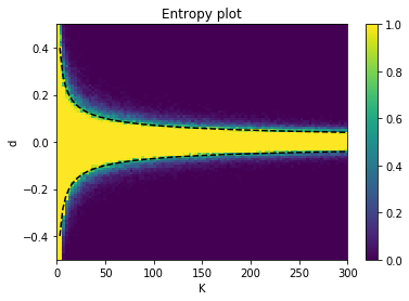
Fig. 1: Values of $\overline{H}$ for different configurations of the asymmetry and the mean degree. The experiment shows a good agreement with the predicted EoC region (dashed line), where we observe an abrupt change of the entropy from $0$ to $1$.

4.2 Effects of perturbations on state evolution

In order to assess the effect of chaos on the network behavior, we compare the evolution of a bESN instantiated with weight matrix $\boldsymbol{W}$ but different initial conditions. Starting from a random initial condition, we generated $50$ additional initial conditions by flipping the state of a single neuron (as in Sec. 3.1). Here, an initial condition $\boldsymbol{x}_{0}$ is randomly generated with a biased probability $c=0.6$ for a neuron to assume a positive value. We let the original and perturbed networks evolve, and take into account the (normalized) Hamming distance, $D_{H}$, between trajectories.

Results are summarized in Fig. 2. We observe that, in the ordered phase, perturbations on the initial state have no effect on the network evolution and the Hamming distance of the perturbed trajectory from the original one is zero. As $d$ decreases (i.e., the networks approach the chaotic regime), we observe how the Hamming distance significantly increases, leading to chaos. Note that the maximum value achievable by the (normalized) Hamming distance is $0.5$, corresponding to the distance of two random binary vectors (a larger distance would imply a negative correlation). In the same set of figures, we show three additional indicators, called Energy, Activity, and Entropy. The mean Energy, defined as $E(\boldsymbol{x}[n]):=\frac{1}{N}\sum_{i=1}^{N}x_{i}[n]$, quantifies the average number of positive and negative neurons. In the frozen phase, the network almost instantly evolves towards values close to $1$ (cfr. the role of $c$, discussed above), and then rapidly decreases to $0$, which is the expected value in the chaotic phase. The mean Activity of network at time-step $n$ is defined as the (normalized) Hamming distance of the current state w.r.t the previous one, $A(\boldsymbol{x}[n])=D_{H}(\boldsymbol{x}[n],\boldsymbol{x}[n-1])$, i.e., the number of neurons that changed their states in one step. As expected, networks operating in chaotic regimes are characterized by an elevated activity. Lastly, we plot the evolution of the Entropy (8) over time. As expected from the theory, transitioning to a chaotic regime is signaled by a sharp increase of entropy.

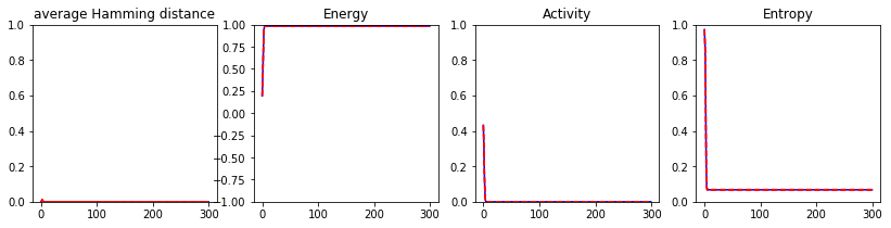
(a) $d=0.25$

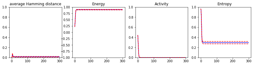
(b) $d=0.184$

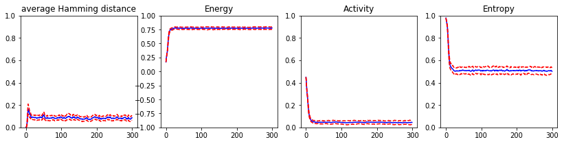
(c) $d=0.157$

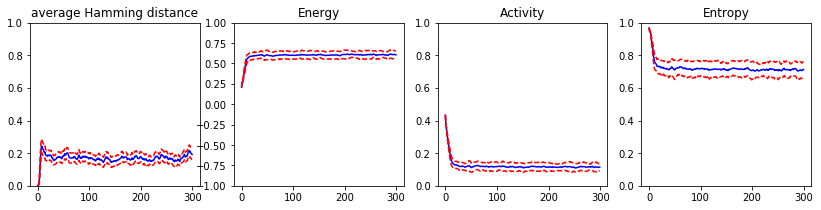
(d) $d=0.144$

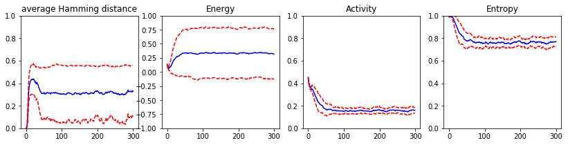
(e) $d=0.131$

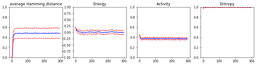
(f) $d=0.105$

Fig. 2: Mean values of the Hamming distance, Energy, Activity and Entropy of the $50$ perturbed networks, with $N=1000$ and $K=22$ for selected values of $d$ (see 4.2). The $x$-axis represents time. The values of the quantities are plotted in blue, while the dashed red lines show the variance. The predicted system should turn chaotic for $d<1/\sqrt{2\langle k\rangle}\approx 0.15$ , according to the theoretical formula.

4.3 Impact of noise in bESN edge of chaos

Here, we study how the EoC is influenced when considering an independent noise term for each neuron, $x_{i}[n+1]=\operatorname{sgn}\!\left(S_{i}[n]+\nu\!\cdot\!\langle k\rangle\!\cdot\!\xi_{i}[n]\right)$, where $\nu$ is the noise gain, $\xi_{i}\sim\mathcal{N}(0,1)$, and $S_{i}$ is the same as in Eq.(4). The choice of scaling the noise with $\langle k\rangle$ was made to account for the fact that the network stability increases with it, as we discuss below.

To explore the dependency from $\nu$, we ran an experiment where we fixed $\langle k\rangle$ and plotted $\nu$ versus $d$. Results are shown in Fig. 3. We can recognize three regimes: (1) for low noise values, the chaotic region remains almost constant; (2) for intermediate values, the chaotic region linearly expands with the noise intensity up until (3) there is only chaos. We repeated the experiments with different values of $\langle k\rangle$ (not shown) and they all confirm the same linear expansion of the chaotic region (in units of $\langle k\rangle$).

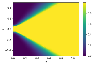
Fig. 3: Values of $\overline{H}$ for different configurations of $d$ and the $\nu$. Note that $\nu$ is multiplied by the mean degree, which is here fixed to $\langle k\rangle=200$.

To verify this fact for a wider range of $\langle k\rangle$, we repeated the experiment in Fig. 1 with noise intensity $\nu=0.1$. It is possible to observe in Fig. 4 how the EoC maintains its shape for lower values of $\langle k\rangle$, while for higher average degrees it deviates from the theoretical prediction and the chaotic region depends on $d$ only.

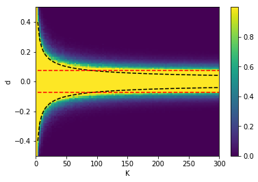
Fig. 4: The same experiment of Fig.1, but with the presence of a noise term with $\nu=0.1$ (multiplied by the mean degree, so that it increases along the $x$-axis). Note how for higher degree the chaos region is constant (the predicted value is the red dashed line), deviating from the autonomous-case prediction (red dashed line).

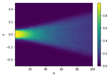
Fig. 5: Network driven by white noise. Values of $\overline{H}$ for different configurations of $A$ and $d$. The mean degree was fixed to $\langle k\rangle=150$.

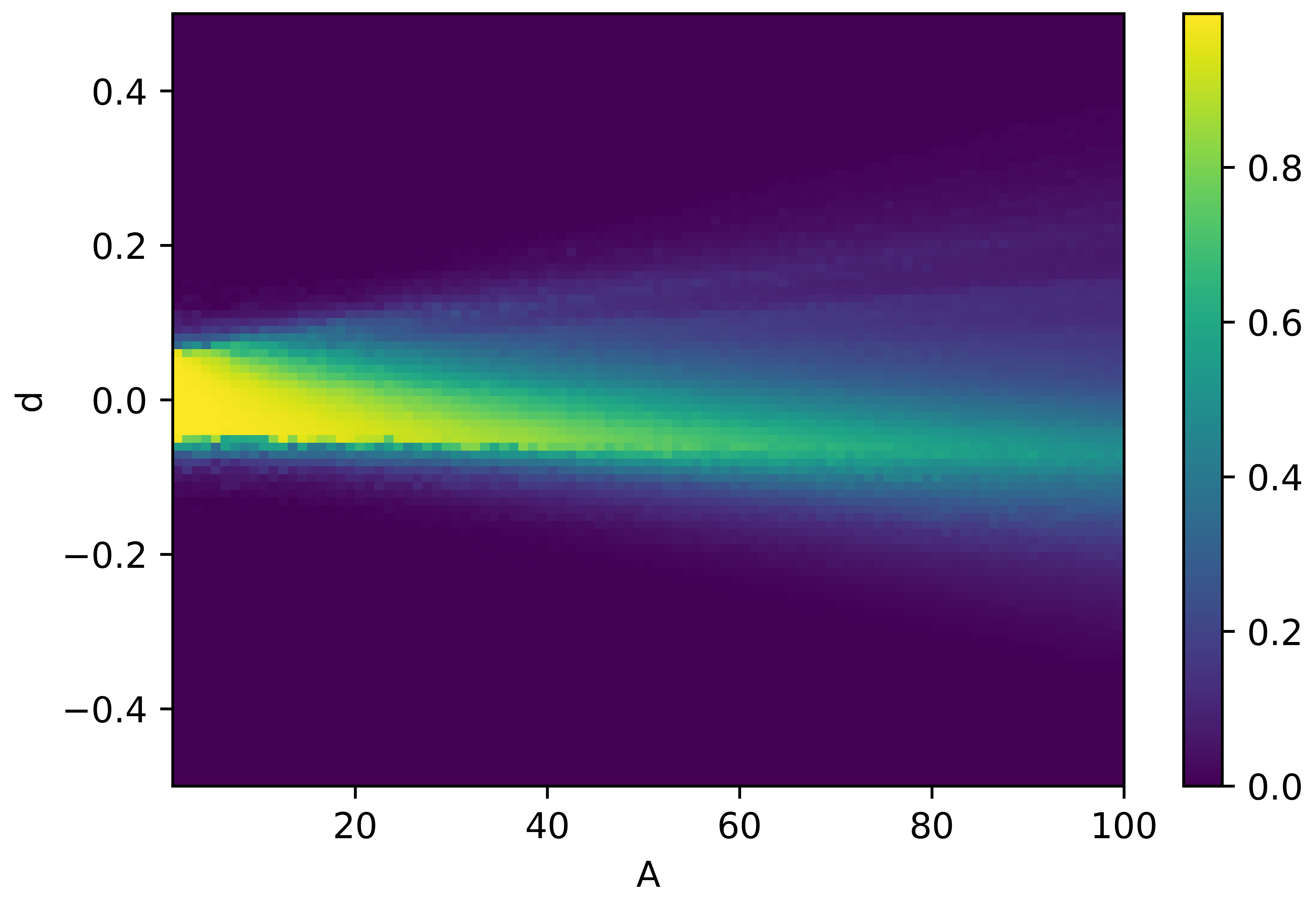
Fig. 6: Network driven with the sum of three sinusoids. Values of $\overline{H}$ for different configurations of $A$ and $d$. The mean degree was fixed to $\langle k\rangle=150$.

We explain this fact as follows. Neurons can only assume $1$ or $-1$ values. The probability of a neuron having $j$ positive inputs is then $P_{k}(j)={\binom{k}{j}}p^{j}q^{k-j}$ where $k$ is its in-degree. If we consider that $j\!=\!\frac{k+s}{2}$, where $s$ is the value of the sum of the positive and negative inputs (whose sign determines the value of the neuron), then we obtain $s\!=\!2j-k$. The expectation of $j$ is $\langle j\rangle\!=\!pk$, so that the expectation of $s$ and its variance are:

$$\langle s\rangle=k(p-q)=2kd$$ (9)

$$\langle(s-\langle s\rangle)^{2}\rangle=4kpq=k(1-4d^{2})$$ (10)

Note that these values are related to a single neuron. For a general understanding of the network behavior, one simply uses $\langle k\rangle$ instead of $k$ in the expressions above, so that it is possible to consider $\sigma^{2}:=\langle k\rangle(1-4d^{2})$ as a mean-field variance of the total inputs to neurons. The impact of the noise on the network can then be studied considering the ratio between $\nu$ and $\sigma^{2}$. As previously discussed, the noise expands the chaos region linearly with its $\nu$.

The noise we are considering has a standard deviation $\theta_{k}=\nu\!\cdot\!\langle k\rangle$. This leads us to a formula for the chaotic region which, for $\langle k\rangle\gg 1$, is $|d|<a\cdot\nu+b$. This relation, as shown in Fig. 4, does not depend on $\langle k\rangle$. As such, having Gaussian noise with standard deviation $\theta$, the formula is $|d|<a\cdot\frac{\theta}{\langle k\rangle}$, or in terms of $\langle k\rangle$, we have $\langle k\rangle<k_{c}^{\textup{noise}}:=\frac{a\theta}{|d|}$. In our experiments, constant $a$ was determined as $a\approx 0.65$.

4.4 Impact of a signal

As for the noise, the magnitude of the signal should have a major role in the EoC, but this time the chaotic region should reduce instead of expanding, since the signal is known to suppress chaos in certain conditions [11]. The signal introduces a correlation among neurons, which makes the annealed approximation ineffective. We drive the network with the signal as in (4), but we scale $u[n]$ with a gain factor $A$, since we are interested in its usage as an hyperparameter and not in relation with $\langle k\rangle$. We initially feed the network with white noise (note that this is different from what we did in 4.3, since in this case the noise is the same for each neuron): from Fig. 5 one can observe how the chaotic region rapidly shrinks as $A$ increases, but a region with an intermediate value of entropy expands (linearly). This is due to the fact the signal prevents the system from collapsing in a stable state, keeping the entropy above zero.

In Fig.6 we show the results obtained for the normalized sum of three sines with incommensurable frequencies (repeated also with different numbers of sinudoids, not shown). Again we note how the chaotic region shrinks as $A$ increases, with the appearance of the region characterized by intermediate entropy values which, instead, expands.

5 Conclusions

The binary ESN model herein introduced is in principle similar to regular ESNs. However, its simplicity permits a theoretical analysis of some important aspects of the transition to chaos. The expression we derived here for the autonomous case perfectly matches the experimental results. Our analysis of the noise applied to neuron activations showed how the network stability increases linearly with the mean degree of recurrent connections. The effects of input signals on the network dynamics are more complex to understand, since they introduce correlations among neurons. Our analysis partially explained the role that the signal magnitude and the mean degree play in shaping the EoC of the non-autonomous case.

References

- [1] Carlo Baldassi et al. “Learning may need only a few bits of synaptic precision” In Physical Review E 93.5 APS, 2016, pp. 052313
- [2] Yu Cheng, Duo Wang, Pan Zhou and Tao Zhang “Model Compression and Acceleration for Deep Neural Networks: The Principles, Progress, and Challenges” In IEEE Signal Processing Magazine 35.1 IEEE, 2018, pp. 126–136 DOI: 10.1109/MSP.2017.2765695
- [3] Bernard Derrida and Yves Pomeau “Random networks of automata: a simple annealed approximation” In EPL (Europhysics Letters) 1.2 IOP Publishing, 1986, pp. 45
- [4] Farzad Farkhooi and Wilhelm Stannat “Complete Mean-Field Theory for Dynamics of Binary Recurrent Networks” In Physical review letters 119.20 APS, 2017, pp. 208301
- [5] Claudio Gallicchio and Alessio Micheli “Echo State Property of Deep Reservoir Computing Networks” In Cognitive Computation Springer, 2017, pp. 1–14
- [6] Herbert Jaeger “The “echo state” approach to analysing and training recurrent neural networks-with an erratum note” In Bonn, Germany: German National Research Center for Information Technology GMD Technical Report 148.34, 2001, pp. 13
- [7] S A Kauffman “Metabolic stability and epigenesis in randomly constructed genetic nets” In Journal of theoretical biology 22.3 Elsevier, 1969, pp. 437–467
- [8] Chris G Langton “Computation at the edge of chaos: phase transitions and emergent computation” In Physica D: Nonlinear Phenomena 42.1-3 Elsevier, 1990, pp. 12–37
- [9] Robert Legenstein and Wolfgang Maass “Edge of chaos and prediction of computational performance for neural circuit models” In Neural Networks 20.3 Elsevier, 2007, pp. 323–334
- [10] Lorenzo Livi, F M Bianchi and Cesare Alippi “Determination of the edge of criticality in echo state networks through Fisher information maximization” In IEEE Transactions on Neural Networks and Learning Systems 29.3, 2018, pp. 706–717 DOI: 10.1109/TNNLS.2016.2644268
- [11] Kanaka Rajan, L F Abbott and Haim Sompolinsky “Stimulus-dependent suppression of chaos in recurrent neural networks” In Physical Review E 82.1 APS, 2010, pp. 011903
- [12] Alexander Rivkind and Omri Barak “Local dynamics in trained recurrent neural networks” In Physical Review Letters 118.25 APS, 2017, pp. 258101
- [13] Thimo Rohlf and Stefan Bornholdt “Criticality in random threshold networks: annealed approximation and beyond” In Physica A: Statistical Mechanics and its Applications 310.1-2 Elsevier, 2002, pp. 245–259
- [14] X R Wang, J T Lizier and Mikhail Prokopenko “Fisher information at the edge of chaos in random Boolean networks” In Artificial Life 17.4 MITP, 2011, pp. 315–329
- [15] I B Yildiz, Herbert Jaeger and S J Kiebel “Re-visiting the echo state property” In Neural Networks 35 Elsevier, 2012, pp. 1–9