Auction Theory Adaptations for Real Life Applications

Ravi Kashyap

Keywords: Auction; First Price Sealed Bid; Strategy; Valuation; Uncertainty; Log-normal

JEL Codes: D44 Auctions; G17 Financial Forecasting and Simulation, C73 Stochastic and Dynamic Games

March 19, 2024

Edited Version: Kashyap, R. (2018). Auction Theory Adaptations for Real Life Applications. Research in Economics, 72(4), 452-481.

1  Abstract

We develop extensions to auction theory results that are useful in real life scenarios.

1. Since valuations are generally positive we first develop approximations using the log-normal distribution. This would be useful for many finance related auction settings since asset prices are usually non-negative.

2. We formulate a positive symmetric discrete distribution, which is likely to be followed by the total number of auction participants, and incorporate this into auction theory results.

3. We develop extensions when the valuations of the bidders are interdependent and incorporate all the results developed into a final combined realistic setting.

4. Our methods can be a practical tool for bidders and auction sellers to maximize their profits. The models developed here could be potentially useful for inventory estimation and for wholesale procurement of financial instruments and also non-financial commodities.

All the propositions are new results and they refer to existing results which are stated as Lemmas.

2 Auction Strategy

Auctions are widely used to transact in goods and services, when a price for the exchange is not readily available before the auction process is set in motion. Recorded history mentions auctions being held as early as 500 B.C (Doyle & Baska 2014; End-note 3). The collection of works on Auction Theory is vast and deep: (Vickrey 1961) is credited with having initiated the study of auctions as games of incomplete information. (Fudenberg & Tirole 1991; Osborne & Rubinstein 1994) are comprehensive references for the study of games and economic behavior.

(Klemperer 1999) is an extensive survey of the enormous literature regarding auctions; (Milgrom 1989) is an excellent introduction to the topic and has sufficient technical details to provide a rigorous yet succinct foundation; other classic surveys are (McAfee & McMillan 1987a; Wilson 1992). (Wilson 1979) compares the sale prices when the item is sold to the highest bidder and when the bidders receive fractional shares of the item at a sale price that equates demand and supply of shares. Auction situations with multiple related objects being sold are considered in (Milgrom 1985; Hausch 1986; Armstrong 2000; Ausubel 2004).

The core results have been extended to applications in transportation, telecommunication, network flow assignment, E-commerce, pricing mechanism for electric power, biological organ transplants (Bertsekas 1988; Post, Coppinger & Sheble 1995; McMillan 1995; Tuffin 2002 ; Gregg & Walczak 2003; Sheffi 2004; Roth, S nmez & nver 2004), among other areas, covering both cooperative and competitive aspects of designing mechanisms to ensure efficient exchange and usage of resources. A few recent extensions, (Di Corato, Dosi & Moretto 2017) study how exit options can affect bidding behavior; (Pica & Golkar 2017) develop a framework to evaluate pricing policies of spacecraft trading commodities, such as data routing, in a federated satellite network. While most extensions to the basic auction theory results are extremely elegant and consider complex scenarios; the daily usage of auctions requires assumptions regarding the number of total bidders and how the valuations of the different bidders might be distributed. We provide fundamental extensions, which will be immediately applicable in real life situations.

We consider a few variations in the first price sealed bid auction mechanism. Once a bidder has a valuation, it becomes important to consider different auction formats and the specifics of how to tailor bids, to adapt, to the particular auction setting. A bidding strategy is sensitive to assumed distributions of both the valuations and the number of bidders. We build upon existing results from the following standard and detailed texts on this topic, which act as the foundation: (Klemperer 2004; Krishna 2009; Menezes & Monteiro 2005; and Milgrom 2004). Additional references are pointed out in the relevant sections below along with the extensions that are derived.

The primary distribution we study is the log-normal distribution (Norstad 1999). The log-normal distribution centers around a value and the chance of observing values further away from this central value become smaller. Asset prices are generally modeled as log-normal, so financial applications (Back & Zender 1993, Nyborg & Sundaresan 1996 are discussions about auctions related to treasury securities; Kandel, Sarig & Wohl 1999, Biais & Faugeron-Crouzet 2002 analyze the auctions of stock initial public offerings; Kashyap 2016 is an example of using auctions for extremely exotic financial products in a complex scenario related to securities lending) would benefit from this extension, with potential applications to other goods that follow such a distribution. The absence of a closed form solution for the log-normal distribution forces us to develop a rough theoretical approximation and improve upon that significantly using non linear regressions.

As a simple corollary we consider the uniform distribution, since the corresponding results can act as a very useful benchmark. The uniform distribution is well uniform and hence is ideal when the valuations (or sometimes even the number of bidders) are expected to fall equally on a finite (or even infinite) number of possibilities. This serves as one extreme to the sort of distribution we can expect in real life. The two distribution types we discuss can shed light on the other types of distributions in which only positive observations are allowed. The regression based numerical technique that we have developed can be useful when the valuations are distributed according to other distributions as well.

We formulate a new positive symmetric discrete distribution, which is likely to be followed by the total number of auction participants, and incorporate this into auction theory results. This distribution can also be a possibility for the valuations themselves, since the set of prices of assets or valuations can be a finite discrete set. But given the results for the discrete distribution of auction participants, developing a bidding strategy based on discrete valuations is trivial and hence is not explicitly given below. Lastly, the case of interdependent valuations is to be highly expected in real life (Kashyap 2016 is an example of such a scenario from the financial services industry); but practical extensions for this case are near absent. We develop extensions when the valuations of bidder are interdependent and incorporate all the results developed into a final combined realistic setting.

We provide proofs for the extensions but we also state standard results with proofs so that it becomes easier to see how the extensions are developed. Such an approach ensures that the results are instructive and immediately applicable to both bidders and auction facilitators. All the propositions are new results and they refer to existing results which are given as Lemmas. The results developed here can be an aid for profit maximization for bidders and auctions sellers during the wholesale procurement of financial instruments and also non-financial commodities.

We define all the variables as we introduce them in the text but section 7 has a complete dictionary of all the notation and symbols used in the main results.

2.1 Symmetric Independent Private Values with Valuations from General Distribution

As a benchmark bidding case, it is illustrative to assume that all bidders know their valuations and only theirs and they believe that the values of the others are independently distributed according to the general distribution $F$. $x_{i}$ is the valuation of bidder $i$. This is a realization of the random variable $X_{i}$ which bidder $i$ and only bidder $i$ knows for sure. $x_{i}\sim F\left[0,\omega\right]$, $x_{i}$ is symmetric and independently distributed according to the distribution $F$ over the interval $\left[0,\omega\right]$. $F,$ is increasing and has full support, which is the non-negative real line $\left[0,\infty\right]$, hence in this formulation we can have $\omega=\infty$. $f=F^{\prime},$ is the continuous density function of $F$. $M,$ is the total number of bidders. When there is no confusion about which specific bidder we are referring to, we drop the subscripts such as in the valuation $x$. $Y_{1}\equiv Y_{1}^{M-1}$ , is the random variable that denotes the highest value, say for bidder 1, among the $M-1$ other bidders. $Y_{1},$ is the highest order statistic of $X_{2},X_{3},...,X_{M}$. $G,$ is the distribution function of $Y_{1}$. That is, $\forall y,\;G(y)=\left[F(y)\right]^{M-1}$and $g=G^{\prime},$ is the continuous density function of $G$ or $Y_{1}$. $m\left(x\right),$ is the expected payment of a bidder with value $x$. $\beta_{i}:\left[0,\omega\right]\rightarrow\Re_{+}$ is an increasing function that gives the strategy for bidder $i$. We let $\beta_{i}\left(x_{i}\right)=b_{i}$. We must have $\beta_{i}\left(0\right)=0$. $\beta:\left[0,\omega\right]\rightarrow\Re_{+}$ is the strategy of all the bidders in a symmetric equilibrium. We let $\beta\left(x\right)=b$. We also have $b\leq\beta\left(x\right)\;\text{and}\;\beta\left(0\right)=0$.

Lemma 1.

The symmetric equilibrium bidding strategy for a bidder, the expected payment of a bidder and the expected revenue of a seller are given by

Equilibrium Bid Function is,

$$\beta\left(x\right) = \left[x-\int_{0}^{x}\left[\frac{F\left(y\right)}{F\left(x\right)}\right]^{M-1}dy\right]$$

Expected ex ante payment of a particular bidder is,

$$E\left[m\left(x\right)\right] = \int_{0}^{\omega}y\left[1-F\left(y\right)\right]g\left(y\right)dy$$

Expected revenue, $R_{s}$, to the seller is

$$E\left[R_{s}\right]=ME\left[m\left(x\right)\right]$$

Proof.

Appendix 8.1. ∎

2.2 Symmetric Independent Private Values with Valuations Distributed Log-normally

Proposition 1.

The symmetric equilibrium bidding strategy when the valuations are small, of the order less than one, and distributed log-normally, can be roughly approximated as

$$\beta\left(x\right) = \left[x-\frac{\int_{0}^{x}\left[\Phi\left(\frac{\ln y-\mu}{\sigma}\right)\right]^{M-1}dy}{\left[\Phi\left(\frac{\ln x-\mu}{\sigma}\right)\right]^{M-1}}\right]$$

$$\approx \frac{x}{2}$$

Here, $\Phi(u)=\frac{1}{\sqrt{2\pi}}\int_{-\infty}^{u}e^{-t^{2}/2}dt$ , is the standard normal cumulative distribution and $X=e^{W}$where, $W\sim N\left(\mu,\sigma\right)$. $x_{i}\sim LN\left[0,\omega\right]$ since we are considering the log-normal distribution.

Proof.

Appendix 8.2. ∎

We see that the log-normal approximation based on the theoretical approximation (Proposition 1), does not depend on the number of bidders and we provide a possible explanation for this counter intuitive result below [it is interesting to compare the bidding strategy in the two cases, uniform (Corollary 1 below) and log-normal distribution (Proposition 1), with regards to the number of bidders]. This theoretical approximation is valid only for small values of the parameters of the order of less than one and the region of validity is limited due to the fact that the left limit of the bid strategy expression does not exist at $x=0.$

Clearly, numerical integration of the expression for the bid strategy from (Proposition 1 or Lemma 1) is a feasible option to obtain the final results. But the drawback with this approach is that it is not immediately obvious how sensitive the bid strategy is to the valuation, the parameters of the valuation distribution and the number of bidders. An in-depth numerical integration analysis would be able to develop sensitivity measures, but the users of the final results are not in anyway required to know or even be familiar with the sensitivities when they use the results. This sensitivity is highly useful in real-life scenarios when bidders have to estimate the parameters and hence knowing the sensitivity can possibly help to counter the extent of uncertainties associated with the estimates. Also, numerical integration reveals that the theoretical approximation is quite sensitive to the parameters at different regions of the solution space.

Hence, to obtain an expression for the bid strategy that depends on the parameters, we resort to numerically calculating (using numerical integration) the bid expression for a sample of parameters that are simulated from appropriate distributions. We draw samples for the valuation and the valuation distribution parameters from folded normal distributions. To get the number of bidders, we set an appropriate ceiling for the values drawn from a folded normal distribution so that the number of bidders is an integer value greater than or equal to two. We then run non-linear power regressions, of the form shown in (eq 1), with the numerically calculated bid strategy values as the dependent variable and the valuation, the valuation distribution parameters and the number of bidders as independent variables.

Remark 1.

A better approximation can be obtained using non-linear regression to find the constant, $C$, and the power coefficients, $a_{1}$,$a_{2}$,$a_{3}$ and $a_{4}$ in the expression below,

$$\beta\left(x\right)=Cx^{a_{1}}\mu^{a_{2}}\sigma^{a_{3}}M^{a_{4}}$$ (1)

The regression coefficients: the constant, $C$, the power coefficients, $a_{1}$,$a_{2}$,$a_{3}$ and $a_{4}$ in (eq 1) are summarized in figure 1 (columns: propConst, valuationP, valMeanP, valStdDevP, biddersMP). The correlation between the bid strategy values using numerical integration and both in-sample and out of sample results from using the regression expression (eq 1) are also shown in figure 1 (columns: powerCorr, osPCorr), along with the sample size and a variable that is proportional to the standard deviation of the folded normal distributions (columns: sampleSize, accuParam).

$$\beta\left(x\right)=\beta_{0}+\beta_{1}x+\beta_{2}\sigma+\beta_{3}\mu+\beta_{4}\left(M-1\right)+...+\beta_{l}x^{k}+\beta_{l+1}\sigma^{k}+...$$ (2)

As seen from the above expression (eq 2), linear regressions are not a good choice in this case since some of the regression coefficients can be negative and this can result in negative values for the bid strategy. We still report some basic results for the linear regression (Figure 1, column: linearCorr, gives the correlations between the bid strategy using numerical integration and results when using a first order regression of the form eq 2) since it acts as a benchmark to provide a good comparison for non-linear regressions, that give better results. Including higher order terms for the parameters still has the same issue of possibly getting negative values for the bid strategy and does not increase the accuracy of the approximation, based on some trials that we conducted.

Figure 1: Non-Linear Regression Coefficients and Accuracy

From figure 1, we find that $a_{1}$, which is the coefficient for the valuation $x$, is the most significant one indicating that the bid strategy is very sensitive to the valuation and does not depend that much on the other parameters. This is possibly an explanation for the theoretical approximation that only involves the valuation in Proposition 1. We see that the power regression produces a more accurate fit than the linear regression. The power expression is also more accurate for smaller values of the parameters, say of the order less than one, and when the number of bidders is more. The lesser the standard deviation of the valuation distribution, the more accurate the approximation results. But when the standard deviation of the parameter distributions is high, the power regression outperform the linear regression. We do not see a significant difference between the coefficients and the accuracy of the fit whether we use $M$ or $M-1$ in the regressions.

Figure 2 gives some raw values of the bid strategy from the numerical integration (dependent variable) in the first column and the parameters it depends on, including the linear regression fit of the first order and the fit from the non-linear regression; (these independent variables: the valuation, the valuation distribution mean and standard deviation and the number of bidders are shown in the subsequent columns, second to fifth columns respectively; the sixth and seventh columns are the regression results from the linear and power regressions; the eight column is the ratio of the numerator and denominator in Proposition 1, which is also the equivalent of the valuation minus the bid strategy; the last three columns give the ratio of the valuation and the bid strategy using numerical integration, the ratio of the bid strategy using numerical integration and the power regression result and the ratio of bid strategy using numerical integration and the linear regression result).

Across the entire sample (almost 220,000 observations), the correlation between the linear regression fit and the bid strategy and the valuation are 0.34 and 0.35 respectively; the correlation between the power regression fit and the bid strategy and the valuation are 0.99 and 0.99 respectively. This shows with a certain degree of clarity that the power regression fit is a better model. A detailed analysis of the variance explained by both models at different regions of the parameter space can help in establishing the superiority of the power model. Such an undertaking can be based on the specifics of the auction situation and such a more thorough comparison can be useful in deciding which model to use and related practical considerations.

An immediately obvious fact is that, $\forall x,\beta\left(x\right)\leq x$. This suggests that fitting different non-linear regression equations for different buckets of values of $x$ can improve the overall accuracy of the results. Though we need to be aware of and watch out for the statistical fact that over-fitting might improve accuracy of the fit but might not necessarily improve the predictive power. Hence, we need to perform out of sample tests for any models we fit before we deem the models to be providing an improvement. Lastly, it should be clear that the regression based technique is very powerful and can be applicable in many situations. Fitting a regression equation of the form in (Eq. 1) can be useful even when the valuations follow other complex distributions, with suitable modifications to factor in the corresponding distribution parameters as independent variables. We could even introduce other independent variables to capture the auction environment such as the industry, the extent of competition within an industry, any constraints being faced by the auction sellers and so on.

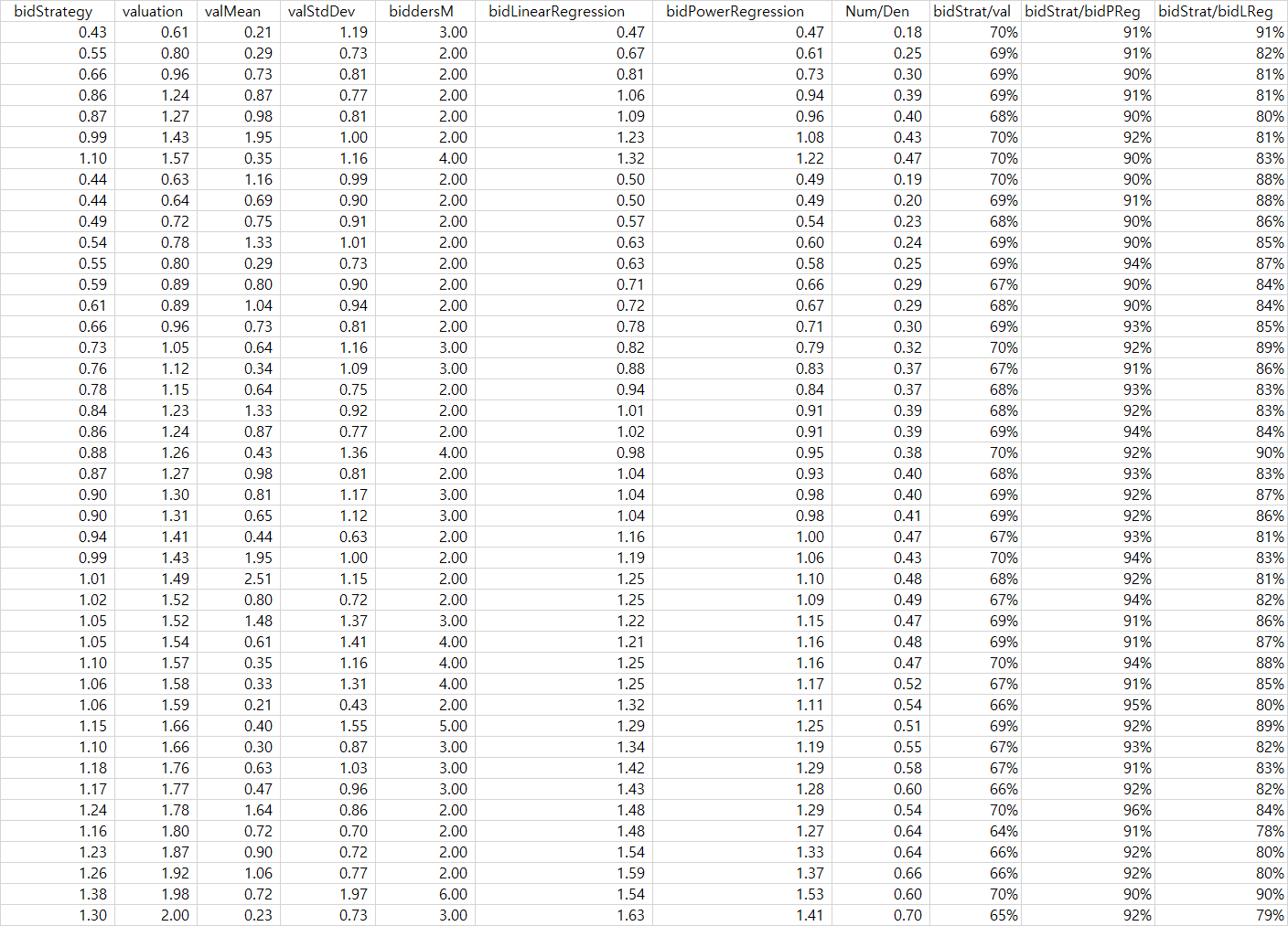
Figure 2: Bid Strategy, Parameter Samples and Regression Results

2.3 Symmetric Independent Private Values with Valuations Distributed Uniformly

Corollary 1.

The symmetric equilibrium bidding strategy when the valuations are distributed uniformly is given by

$$\beta\left(x\right) = \left(\frac{M-1}{M}\right)x$$

Here, $x_{i}\sim U\left[0,\omega\right]$ since we are considering the uniform distribution.

Proof.

Appendix 8.3. ∎

When the number of bidders are large the above expression for the uniform distribution does not depend on the number of bidders, that is $\underset{M\rightarrow\infty}{\lim}\left(\frac{M-1}{M}\right)x=x$. Comparing the bidding strategy with respect to the distribution of valuations in the two cases, the uniform distribution when the number of bidders are large and the log-normal distribution theoretical approximation (Proposition 1) we see that: 1) both do not depend significantly on the number of bidders and 2) the bid is larger with a uniform distribution.

2.4 Symmetric Independent Private Value with Reserve Prices

Lemma 2.

The symmetric equilibrium bidding strategy when the valuation is greater than the reserve price, $\left(r>0\right)$, of the seller, $x\geq r$, is

For a general distribution,

$$\beta\left(x\right) = r\frac{G\left(r\right)}{G\left(x\right)}+\frac{1}{G\left(x\right)}\int_{r}^{x}yg\left(y\right)dy$$

$$\text{Alternately }\beta\left(x\right) = x-\int_{r}^{x}\frac{G\left(y\right)}{G\left(x\right)}dy$$

Proof.

Appendix 8.4. ∎

2.4.1 Uniform Distributions

Corollary 2.

The symmetric equilibrium bidding strategy when the valuation is greater than the reserve price of the seller, $x\geq r$, and valuations are from an uniform distribution,

$$\beta\left(x\right)=\frac{r^{M}}{x^{M-1}}\left(\frac{M+1}{M}\right)+x\left(\frac{M-1}{M}\right)$$

Proof.

Appendix 8.5. ∎

2.4.2 Log-normal Distributions

Corollary 3.

The symmetric equilibrium bidding strategy when the valuation is greater than the reserve price of the seller, $x\geq r$, and valuations are from a log-normal distribution,

$$\beta\left(x\right)=x\left[\frac{h^{\prime}\left(r\right)\left(x-r\right)}{h\left(x\right)}+\frac{r}{x}\frac{h\left(r\right)}{h\left(x\right)}\right]$$

$$\text{Here, }h^{\prime}\left(r\right)=\left(M-1\right)\left[\int_{-\infty}^{\left(\frac{\ln r-\mu}{\sigma}\right)}e^{-t^{2}/2}dt\right]^{M-2}\left\{\frac{e^{-\left(\frac{\ln r-\mu}{\sigma}\right)^{2}/2}}{r\sigma}\right\}$$

Proof.

Appendix 8.6. ∎

We can obtain decent approximations using non-linear power regressions, of the form shown in (eq 1), with the numerically calculated bid strategy values as the dependent variable and the valuation, the valuation distribution parameters, the reserve price and the number of bidders as independent variables.

2.4.3 Optimal Reserve Price for Seller and Other Considerations

Lemma 3.

The optimal reserve price for the seller, $r^{*}$ must satisfy the following expression,

$$x_{s}=r^{*}-\frac{\left[1-F\left(r^{*}\right)\right]}{f\left(r^{*}\right)}$$

Here, seller has a valuation, $x_{s}\in\left[0,\omega\right)$ t

Proof.

Appendix 8.7. ∎

2.5 Variable Number of Bidders with Symmetric Valuations and Beliefs about Number of Bidders

$\mathcal{M}=\left\{1,2,\ldots,M\right\}$ is the potential set of bidders when there is uncertainty about how many interested bidders there are. $\mathcal{A}\subseteq\mathcal{M}$ is the set of actual bidders. All potential bidders draw their valuations independently distributed according to the general distribution $F$. Also, $p_{l}$ is the probability that any participating bidder, $i\in\mathcal{A},$ is facing $l$ other bidders or the probability that he assigns to the event that he is facing $l$ other bidders. This implies that there is a total of $l+1$ bidders, $l\in\left\{1,2,\ldots,M-1\right\}$. $G^{l}\left(x\right)=\left[F\left(x\right)\right]^{l}$ is the probability of the event that the highest of $l$ values drawn from the symmetric distribution $F$ is less than $x$, his valuation and the bidder wins in this case. $\beta^{l}\left(x\right)$ is the equilibrium bidding strategy when there are a total of exactly $l+1$ bidders, known with certainty. The overall probability that the bidder will win when he bids $\beta^{M}\left(x\right)$ is

$$G\left(x\right)=\sum_{l=0}^{M-1}p_{l}G^{l}\left(x\right)$$

Hence the equilibrium bid for an actual bidder when he is unsure about the number of rivals he faces is a weighted average of the equilibrium bids in an auction when the number of bidders is known to all. (McAfee & McMillan 1987b) is one of the most well known and early generalizations to allow the number of bidders to be stochastic.

Lemma 4.

The equilibrium strategy when there is uncertainty about the number of bidders is given by

$$\beta^{M}\left(x\right) = \sum_{l=0}^{M-1}\frac{p_{l}G^{l}\left(x\right)}{G\left(x\right)}\beta^{l}\left(x\right)$$

Proof.

Appendix 8.8. ∎

Any financial market participant or intermediary, will expect most of the other major players to be bidding at an auction as well. Invariably, there will be some drop outs, depending on their recent bidding activity and some smaller players will show up depending on the specifics of the particular auction. It is a reasonable assumption that all of the bidders hold similar beliefs about the distribution of the number of players. We construct a symmetric discrete distribution of the sort shown in the diagram below (Figure 3). We show that such a distribution satisfies all the properties of a probability distribution function as part of the proof for Proposition 2. It is to be noted that this symmetric discrete distribution comes under the family of triangular distributions (End-note 4). We can easily come up with variations that can provide discrete asymmetric probabilities. For simplicity, we use the uniform distribution for the valuations and set $\omega=1$. The below result follows from a bidding strategy that incorporates the use of the discrete symmetric distribution.

Proposition 2.

The bidding strategy and the formula for the probability of facing any particular total number of bidders under a symmetric discrete distribution would be given by,

$$\beta\left(x\right)=\sum_{l=0}^{M-1}\left(\frac{p_{l}x^{l}}{\sum_{k=0}^{M-1}p_{k}x^{k}}\right)\left(\frac{l}{l+1}\right)x$$

$$p_{l} = \begin{cases}l\Delta_{p}&,\;\text{if}\;\;l\leq\frac{\left(M-1\right)}{2}\\ \left(M-l\right)\Delta_{p}&,\;\text{if}\;\;l>\frac{\left(M-1\right)}{2}\end{cases}$$

$$\Delta_{p}=\left\{\left\lfloor\frac{M^{2}}{4}\right\rfloor\right\}^{-1}$$

We note that $\Delta_{p}$ can also be written as,

$$\Delta_{p}=\frac{1}{\left\{\left\lfloor\frac{\left(M-1\right)}{2}\right\rfloor\left\{\left\lfloor\frac{\left(M-1\right)}{2}\right\rfloor+1\right\}+\left[\left\{\left(\frac{\left(M-1\right)}{2}\bmod 1\right)+\frac{\left(M-1\right)}{2}\right\}\left\{2\left(\frac{\left(M-1\right)}{2}\bmod 1\right)\right\}\right]\right\}}$$

$$\left\lfloor\frac{\left(M-1\right)}{2}\right\rfloor\text{ is the integer floor function, that is, it rounds any number down to the nearest integer. }$$

$$A\bmod B\text{ is the modulo operator, that is, it gives the remainer when }A\text{ is divided by }B.$$

$$\text{When }A\text{ is a fraction less than one and }B\text{ is one, the result is the fraction itself.}$$

Proof.

Appendix 8.9. ∎

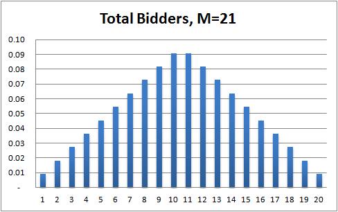
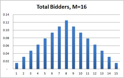
Figure 3: Variable Bidders Symmetric Discrete Probability Distributions

2.6 Asymmetric Valuations

$f_{i},\,F_{i}$ , are the continuous density function and distribution of bidder $i$ in this case where the valuations are asymmetric. $\phi_{i}\equiv\beta_{i}^{-1}$ is the inverse of the bidding strategy $\beta_{i}$. This means, $x_{i}=\beta_{i}^{-1}\left(b_{i}\right)=\phi_{i}\left(b_{i}\right)$. The following result captures the scenario when we have an asymmetric equilibrium.

Lemma 5.

The system of differential equations for an asymmetric equilibrium is given by

$$\sum_{j\neq i}^{j\in\left\{1,...,M\right\}}\left\{\frac{f_{j}\left(\phi_{j}\left(b\right)\right)\phi^{\prime}_{j}\left(b\right)}{F_{j}\left(\phi_{j}\left(b\right)\right)}\right\} = \frac{1}{\left[\phi_{i}\left(b\right)-b\right]}$$

Proof.

Appendix 8.10. ∎

This system of differential equations can be solved to get the bid functions for each player. Closed form solutions are known for the case of uniform distributions with different supports. A simplification is possible by assuming that say, some bidders have one distribution and some others have another distribution. This is a reasonable assumption since financial firms can be categorized into big global and small local companies. Such an assumption can hold even for telecommunication companies or other sectors where local players compete with global players to obtain rights for service to a region or to obtain use of raw materials from a region.

Proposition 3.

If, $K+1$ firms (including the one for which we derive the payoff condition) have the distribution $F_{1}$, strategy $\beta_{1}$ and inverse function $\phi_{1}$. The other $M-K-1$ firms have the distribution $F_{2}$, strategy $\beta_{2}$ and inverse function $\phi_{2}$. The system of differential equations is given by,

$$\left\{K\frac{f_{1}\left(\phi_{1}\left(b\right)\right)\phi^{\prime}_{1}\left(b\right)}{\left[F_{1}\left(\phi_{1}\left(b\right)\right)\right]}\right\}+\left\{\left(M-1-K\right)\frac{f_{2}\left(\phi_{2}\left(b\right)\right)\phi^{\prime}_{2}\left(b\right)}{\left[F_{2}\left(\phi_{2}\left(b\right)\right)\right]}\right\}=\frac{1}{\left[\phi_{i}\left(b\right)-b\right]}$$

Proof.

Appendix 8.11. ∎

As a special case, if there are only two bidders, $M=2,K=1$ the above reduces to a system of two differential equations,

$$\phi^{\prime}_{1}\left(b\right) = \frac{\left[F_{1}\left(\phi_{1}\left(b\right)\right)\right]}{f_{1}\left(\phi_{1}\left(b\right)\right)\left[\phi_{2}\left(b\right)-b\right]}$$

$$\phi^{\prime}_{2}\left(b\right) = \frac{\left[F_{2}\left(\phi_{2}\left(b\right)\right)\right]}{f_{2}\left(\phi_{2}\left(b\right)\right)\left[\phi_{1}\left(b\right)-b\right]}$$

2.7 Symmetric Interdependent Valuations

It is worth noting that a pure common value model of the sort, $V=\upsilon\left(X_{1},X_{2},...,X_{M}\right)$ is not relevant for many entities (firms or individuals) since forces that drive them to participate in auctions might vary. $X_{i}\in\left[0,\omega_{i}\right]$ is bidder $i^{\prime}s$ signal when the valuations are interdependent. $V_{i}=\upsilon_{i}\left(X_{1},X_{2},...,X_{M}\right)$ is the item value to bidder $i$ and $\upsilon_{i}\left(0,0,...,0\right)=0$. $\upsilon_{i}\left(x_{1},x_{2},...,x_{M}\right)\equiv E\left[V_{i}\mid X_{1}=x_{1},X_{2}=x_{2},...,X_{M}=x_{M},\right]$ is a more general setting, where knowing the signals of all bidders still does not reveal the full value with certainty.

In the case of financial firms (Kashyap 2016) the motivation to participate in auctions will depend on their trading activity, which will not be entirely similar, but we can expect many common drivers of trading activity. What this reasoning tells us is that it is reasonable to expect that there is some correlation between the signals of each bidder. This results in a symmetric interdependent auction strategy. From the perspective of a particular bidder, the signals of the other bidders can be interchanged without affecting the value. This is captured using the function $u\left(X_{i},X_{-i}\right)$ which is the same for all bidders and is symmetric in the last $M-1$ components. We assume that all signals $X_{i}$ are from the same distribution $\left[0,\omega\right]$ and that the valuations can be written as

$$\upsilon_{i}\left(X_{1},X_{2},...,X_{M}\right)=u\left(X_{i},X_{-i}\right)$$

We also assume that the joint density function of the signals $f$ defined on $\left[0,\omega\right]^{M}$ is symmetric and the signals are affiliated. Affiliation here refers to the below properties.

• The random variables $X_{1},X_{2},...,X_{M}$ distributed on some product of intervals $\mathcal{X}\subset\Re^{M}$ according to the joint density function $f$. The variables $\mathbf{X=}\left(X_{1},X_{2},...,X_{M}\right)$ are affiliated if $\forall\mathbf{x^{\prime},x^{\prime\prime}}\in\mathcal{X}$, $f\left(\mathbf{x^{\prime}\lor x^{\prime\prime}}\right)f\left(\mathbf{x^{\prime}\land x^{\prime\prime}}\right)\geq f\left(\mathbf{x^{\prime}}\right)f\left(\mathbf{x^{\prime\prime}}\right)$. Here $\mathbf{x^{\prime}\lor x^{\prime\prime}}$ and $\mathbf{x^{\prime}\lor x^{\prime\prime}}$ denote the component wise maximum and minimum of $\mathbf{x^{\prime}}$ and $\mathbf{x^{\prime\prime}}$.

• The random variables $Y_{1},Y_{2},...,Y_{M-1}$ denote the largest, second largest, … , smallest from among $X_{2},X_{3},...,X_{M}$. If $X_{1},X_{2},...,X_{M}$ are affiliated, then $X_{1},Y_{1},Y_{2},...,Y_{M-1}$ are also affiliated.

• Let $G\left(.\mid x\right)$ denote the distribution of $Y_{1}$ conditional on $X_{1}=x$ and let $g\left(.\mid x\right)$ be the associated conditional density function. Then if $Y_{1}$ and $X_{1}$ are affiliated and if $x^{\prime}>x$ then $G\left(.\mid x^{\prime}\right)$ dominates $G\left(.\mid x\right)$ in terms of the reverse hazard rate, $\frac{g\left(t\right)}{G\left(t\right)}$. That is $\forall y$,

  $$\frac{g\left(y\mid x^{\prime}\right)}{G\left(y\mid x^{\prime}\right)}\geq\frac{g\left(y\mid x\right)}{G\left(y\mid x\right)}$$

• If $\gamma$ is any increasing function, then $x^{\prime}>x$ implies that

  $$E\left[\gamma\left(Y_{1}\right)\mid X=x^{\prime}\right]\geq E\left[\gamma\left(Y_{1}\right)\mid X=x\right]$$

We define the below function as the expectation of the value to bidder $1$ when the signal he receives is $x$ and the highest signal among the other bidders, $Y_{1}=y$. Because of symmetry this function is the same for all bidders and we assume it is strictly increasing in $x$. We also have $u\left(\mathbf{0}\right)=\upsilon(0,0)=0$.

$$\upsilon\left(x,y\right)=E\left[V_{1}\mid X=x,Y_{1}=y\right]$$

Lemma 6.

A symmetric equilibrium strategy governed by the set of conditions above is given by

$$\beta\left(x\right)=\int_{0}^{x}\upsilon\left(y,y\right)dL\left(y\mid x\right)$$

Here, we define $L\left(y\mid x\right)$ as a function with support $\left[0,\omega\right]$,

$$L\left(y\mid x\right)=\exp\left[-\int_{y}^{x}\frac{g\left(t\mid t\right)}{G\left(t\mid t\right)}dt\right]$$

Proof.

Appendix 8.12. ∎

Proposition 4.

The bidder’s equilibrium strategy under a scenario when the valuation is the weighted average of his valuation and the highest of the other valuations is given by the expression below. That is, we let $\upsilon\left(x,y\right)=\alpha x+\xi y\;\mid\alpha,\xi\in\left[0,1\right]$. This also implies, $\upsilon\left(x,y\right)=u\left(x,y\right)=u\left(x_{i},x_{-i}\right)=\alpha x_{i}+\xi\max\left(x_{-i}\right)$, giving us symmetry across the signals of other bidders. An alternative formulation could simply be $\upsilon\left(x,y\right)=\frac{1}{M}\left(\overset{M}{\underset{i=1}{\sum}}x_{i}\right)$. The affiliation structure follows the Irwin-Hall distribution (End-note 5) with bidder’s valuation being the sum of a signal coming from a uniform distribution with $\omega=1$ and a common component from the same uniform distribution.

$$\beta\left(x\right) = \left[\frac{2\left(\alpha+\xi\right)\left(M-1\right)}{\left(2M-1\right)x^{2M-2}}\right]$$

$$+ \left(\alpha+\xi\right)\left[x-\frac{1}{\left(2x-1-\frac{x^{2}}{2}\right)^{M-1}}\left\{\frac{1}{2^{M-1}}+\int_{1}^{x}\left(2y-1-\frac{y^{2}}{2}\right)^{M-1}dy\right\}\right]$$

Proof.

The proof in Appendix 8.13 includes a method to solve the last integral. ∎

Despite the simplifications, regarding the distribution assumptions in Proposition 4, being satisfactory approximations in many instances, they have been made to ensure that the results are analytically tractable. More complex distributions can be accommodated using the regression technique we have developed in section 2.2. A regression equation of the form in (Eq. 1) can be used with suitable modifications to introduce other distribution parameters as independent variables.

2.8 Combined Realistic Setting

Proposition 5.

The bidding strategy in a realistic setting with symmetric interdependent, uniformly distributed valuations, with reserve prices and variable number of bidders is given by

$$\beta\left(x\right)=re^{-\int_{x^{*}}^{x}\frac{g\left(t\mid t\right)}{G\left(t\mid t\right)}dt}+\int_{x^{*}}^{x}v(y,y)\frac{g\left(y\mid y\right)}{G\left(y\mid y\right)}e^{-\int_{y}^{x}\frac{g\left(t\mid t\right)}{G\left(t\mid t\right)}dt}dy$$

Here, $x^{*}\left(r\right)$ is found by solving for $x$ in the below condition

$$\left[\int_{0}^{1}\xi y\left[\frac{y}{x}\right]^{2\left(M-2\right)}\left(\frac{2y}{x^{2}}\right)dy+\int_{1}^{x}\xi y\left[\frac{\left(2y-1-\frac{y^{2}}{2}\right)}{\left(2x-1-\frac{x^{2}}{2}\right)}\right]^{M-2}\left\{\frac{2-y}{\left(2x-1-\frac{x^{2}}{2}\right)}\right\}dy\right]=\frac{r-\alpha x}{\left(M-1\right)}$$

Proof.

The proof in Appendix 8.14 includes a method to solve the above type of equations. ∎

It is trivial to extend the above to the case where the total number of bidders is uncertain by using the equilibrium bidding strategy $\beta^{l}\left(x\right)$ and the associated probability $p_{l}$ when there are exactly $l+1$ bidders, known with certainty,

$$\beta^{M}\left(x\right)=\sum_{l=0}^{M-1}\frac{p_{l}G^{l}\left(x\right)}{G\left(x\right)}\beta^{l}\left(x\right)$$

3 Improvements to the Model

We have assumed that the valuation each bidder holds is derived independently before he decides upon his bidding strategy. Instead of the bidding strategies we have considered, we can come up with a parametric model that will take the valuations as the inputs and the bid as output. From a financial industry securities lending perspective (Kashyap 2016), the parameters can depend on the characteristics of the portfolio being auctioned such as, the size of the portfolio, the number of securities, the number of markets, the extent of overlap with the internal inventory, and where available, the percentile rankings of the historical bids for previous auctions, which auction sellers do reveal sometimes. It should be acknowledged, however, that this would be useful if and only if the parametric model is a valid approximation of the general model and the actual auction environment, which may be non-parametric. Therefore, a parametrization may limit the general applicability of any results obtained, though it can be useful for specific applications where the auction setting and the parameters are known to a satisfactory extent. The similarity of the parametric approach to using a regression equation when the valuations follow a particular distribution are to be noted. This suggests that the regression technique can be useful in a variety of situations, where closed form solutions are either absent or not readily obtained.

(Cobb, Rumi & Salmer n 2012; and Nie & Chen 2007) derive approximate distributions for the sum of log-normal distributions which highlight that we can estimate the log-normal parameters from the time series of the valuations and hence get the mean and variance of the valuations. (Norstad 1999) is a basic but excellent reference for the log-normal distribution. A longer historical time series will help get better estimates for the volatility of the valuation. This can be useful to decide the aggressiveness of the bid. Another key extension can be to introduce jumps in the log-normal processes. This is seen in stock prices to a certain extent and to a greater extent in the inventory processes.

4 Conclusion

We have looked at various auction strategy extensions that would be relevant to the application of auctions to many real life situations. All the propositions are new results and they refer to existing results which are given as Lemmas. We have derived the closed form solutions for bidding strategies, relevant to an auction, where such a formulation exists and in situations where approximations would be required, we have provided those. A simple result using the log-normal distribution should be of immense practical use, along with a new positive symmetric distribution that can be used to handle situations where both the valuations and number of bidders are distributed accordingly. The interdependent valuations scenario and the combined realistic setting provide ready to use results for bidders and auction designers alike. These extensions are immediately useful for the auctions of financial securities and should be applicable for numerous other products.

5 Acknowledgements and End-Notes

1. Dr. Yong Wang, Dr. Isabel Yan, Dr. Vikas Kakkar, Dr. Fred Kwan, Dr. William Case, Dr. Srikant Marakani, Dr. Qiang Zhang, Dr. Costel Andonie, Dr. Jeff Hong, Dr. Guangwu Liu, Dr. Andrew Chan, Dr. Humphrey Tung and Dr. Xu Han at the City University of Hong Kong provided advice and more importantly encouragement to explore and where possible apply cross disciplinary techniques. The faculty members of SolBridge International School of Business provided patient guidance and valuable suggestions on how to further this paper.

2. Numerous seminar participants provided helpful suggestions. The views and opinions expressed in this article, along with any mistakes, are mine alone and do not necessarily reflect the official policy or position of either of my affiliations or any other agency.

3. Auction, Wikipedia Link: An auction is a process of buying and selling goods or services by offering them up for bid, taking bids, and then selling the item to the highest bidder.

4. Triangular distribution, Wikipedia Link: In probability theory and statistics, the triangular distribution is a continuous probability distribution with lower limit $a$, upper limit $b$ and mode $c$, where $a<b$ and $a\leq c\leq b$ (also see: Evans, Hastings & Peacock 2000).

5. Irwin–Hall distribution, Wikipedia Link: In probability and statistics, the Irwin–Hall distribution, named after Joseph Oscar Irwin and Philip Hall, is a probability distribution for a random variable defined as the sum of a number of independent random variables, each having a uniform distribution. For this reason it is also known as the uniform sum distribution (also see: Hall 1927; Irwin 1927).

6 References

• Armstrong, M. (2000). Optimal multi-object auctions. The Review of Economic Studies, 67(3), 455-481.

• Ausubel, L. M. (2004). An efficient ascending-bid auction for multiple objects. The American Economic Review, 94(5), 1452-1475.

• Back, K., & Zender, J. F. (1993). Auctions of divisible goods: On the rationale for the treasury experiment. The Review of Financial Studies, 6(4), 733-764.

• Bertsekas, D. P. (1988). The auction algorithm: A distributed relaxation method for the assignment problem. Annals of operations research, 14(1), 105-123.

• Biais, B., & Faugeron-Crouzet, A. M. (2002). IPO auctions: English, Dutch,… French, and internet. Journal of Financial Intermediation, 11(1), 9-36.

• Chiani, M., Dardari, D., & Simon, M. K. (2003). New exponential bounds and approximations for the computation of error probability in fading channels. Wireless Communications, IEEE Transactions on, 2(4), 840-845.

• Cobb, B. R., Rumi, R., & Salmer n, A. (2012). Approximating the Distribution of a Sum of Log-normal Random Variables. Statistics and Computing, 16(3), 293-308.

• Di Corato, L., Dosi, C., & Moretto, M. (2017). Multidimensional auctions for long-term procurement contracts with early-exit options: the case of conservation contracts. European Journal of Operational Research.

• Doyle, R., & Baska, S. (2014). History of Auctions: From ancient Rome to today’s high-tech auctions. Auctioneer, SUA.

• Dyer, D., Kagel, J. H., & Levin, D. (1989). Resolving uncertainty about the number of bidders in independent private-value auctions: an experimental analysis. The RAND Journal of Economics, 268-279.

• Evans, M., Hastings, N., & Peacock, B. (2000). Triangular distribution. Statistical distributions, 3, 187-188.

• Fudenberg, D., & Tirole, J. (1991). Game theory (Vol. 1). The MIT press.

• Gregg, D. G., & Walczak, S. (2003). E-commerce auction agents and online-auction dynamics. Electronic Markets, 13(3), 242-250.

• Hall, P. (1927). The distribution of means for samples of size N drawn from a population in which the variate takes values between 0 and 1, all such values being equally probable. Biometrika, Vol. 19, No. 3/4., pp. 240–245.

• Harstad, R. M., Kagel, J. H., & Levin, D. (1990). Equilibrium bid functions for auctions with an uncertain number of bidders. Economics Letters, 33(1), 35-40.

• Hausch, D. B. (1986). Multi-object auctions: Sequential vs. simultaneous sales. Management Science, 32(12), 1599-1610.

• Huang, H. N., Marcantognini, S., & Young, N. (2006). Chain rules for higher derivatives. The Mathematical Intelligencer, 28(2), 61-69.

• Irwin, J. O. (1927). On the frequency distribution of the means of samples from a population having any law of frequency with finite moments, with special reference to Pearson’s Type II. Biometrika, Vol. 19, No. 3/4., pp. 225–239.

• Johnson, W. P. (2002). The curious history of Fa di Bruno’s formula. American Mathematical Monthly, 217-234.

• Kandel, S., Sarig, O., & Wohl, A. (1999). The demand for stocks: An analysis of IPO auctions. The Review of Financial Studies, 12(2), 227-247.

• Kashyap, R. (2016). Securities Lending Strategies, Exclusive Valuations and Auction Bids. Social Science Research Network. Working Paper.

• Klemperer, P. (1999). Auction theory: A guide to the literature. Journal of economic surveys, 13(3), 227-286.

• Klemperer, P. (2004). Auctions: theory and practice.

• Krishna, V. (2009). Auction theory. Academic press.

• Laffont, J. J., Ossard, H., & Vuong, Q. (1995). Econometrics of first-price auctions. Econometrica: Journal of the Econometric Society, 953-980.

• Lebrun, B. (1999). First price auctions in the asymmetric N bidder case. International Economic Review, 40(1), 125-142.

• Levin, D., & Ozdenoren, E. (2004). Auctions with uncertain numbers of bidders. Journal of Economic Theory, 118(2), 229-251.

• McAfee, R. P., & McMillan, J. (1987a). Auctions and bidding. Journal of economic literature, 25(2), 699-738.

• McAfee, R. P., & McMillan, J. (1987b). Auctions with a stochastic number of bidders. Journal of Economic Theory, 43(1), 1-19.

• McMillan, J. (1995). Why auction the spectrum?. Telecommunications policy, 19(3), 191-199.

• Menezes, F. M., & Monteiro, P. K. (2005). An introduction to auction theory (pp. 1-178). Oxford University Press.

• Milgrom, P. R., & Weber, R. J. (1982). A theory of auctions and competitive bidding. Econometrica: Journal of the Econometric Society, 1089-1122.

• Milgrom, P. R. (1985). The economics of competitive bidding: a selective survey. Social goals and social organization: Essays in memory of Elisha Pazner, 261-292.

• Milgrom, P. (1989). Auctions and bidding: A primer. The Journal of Economic Perspectives, 3(3), 3-22.

• Milgrom, P. R. (2004). Putting auction theory to work. Cambridge University Press.

• Miranda, M. J., & Fackler, P. L. (2002). Applied Computational Economics and Finance.

• Nie, H., & Chen, S. (2007). Lognormal sum approximation with type IV Pearson distribution. IEEE Communications Letters, 11(10), 790-792.

• Norstad, John. "The normal and lognormal distributions." (1999).

• Nyborg, K. G., & Sundaresan, S. (1996). Discriminatory versus uniform Treasury auctions: Evidence from when-issued transactions. Journal of Financial Economics, 42(1), 63-104.

• Ortega-Reichert, A. (1967). Models for competitive bidding under uncertainty. Stanford University.

• Osborne, M. J., & Rubinstein, A. (1994). A course in game theory. MIT press.

• Pica, U., & Golkar, A. (2017). Sealed-Bid Reverse Auction Pricing Mechanisms for Federated Satellite Systems. Systems Engineering.

• Post, D. L., Coppinger, S. S., & Sheble, G. B. (1995). Application of auctions as a pricing mechanism for the interchange of electric power. IEEE Transactions on Power Systems, 10(3), 1580-1584.

• Roth, A. E., S nmez, T., & nver, M. U. (2004). Kidney exchange. The Quarterly Journal of Economics, 119(2), 457-488.

• Sheffi, Y. (2004). Combinatorial auctions in the procurement of transportation services. Interfaces, 34(4), 245-252.

• Tuffin, B. (2002). Revisited progressive second price auction for charging telecommunication networks. Telecommunication Systems, 20(3), 255-263.

• Vickrey, W. (1961). Counterspeculation, auctions, and competitive sealed tenders. The Journal of finance, 16(1), 8-37.

• Wilson, R. (1979). Auctions of shares. The Quarterly Journal of Economics, 675-689.

• Wilson, R. (1992). Strategic analysis of auctions. Handbook of game theory with economic applications, 1, 227-279.

7 Dictionary of Notation and Terminology for the Auction Strategy

• $x_{i}$, the valuation of bidder $i$. This is a realization of the random variable $X_{i}$ which bidder $i$ and only bidder $i$ knows for sure.

• $x_{i}\sim F\left[0,\omega\right]$, $x_{i}$ is symmetric and independently distributed according to the distribution $F$ over the interval $\left[0,\omega\right]$.

• $F,$ is increasing and has full support, which is the non-negative real line $\left[0,\infty\right]$.

• $f=F^{\prime},$ is the continuous density function of $F$.

• $x_{i}\sim U\left[0,\omega\right]$ when we consider the uniform distribution.

• $x_{i}\sim LN\left[0,\omega\right]$ when we consider the log-normal distribution.

• $M,$ is the total number of bidders.

• $f_{i},\,F_{i}$ , are the continuous density function and distribution of bidder $i$ in the asymmetric case.

• $r\geq 0$, is the reserve price set by the auction seller.

• $\beta_{i}:\left[0,\omega\right]\rightarrow\Re_{+}$ is an increasing function that gives the strategy for bidder $i$. We let $\beta_{i}\left(x_{i}\right)=b_{i}$. We must have $\beta_{i}\left(0\right)=0$.

• $\phi_{i}\equiv\beta_{i}^{-1}$ is the inverse of the bidding strategy $\beta_{i}$. This means, $x_{i}=\beta_{i}^{-1}\left(b_{i}\right)=\phi_{i}\left(b_{i}\right)$.

• $x_{i}\sim F_{i}\left[0,\omega_{i}\right]$. Here, $x_{i}$ is asymmetric and is independently distributed according to the distribution $F_{i}$ over the interval $\left[0,\omega_{i}\right]$.

• $\beta:\left[0,\omega\right]\rightarrow\Re_{+}$ is the strategy of all the bidders in a symmetric equilibrium. We let $\beta\left(x\right)=b,x$ is the valuation of any bidder. We also have $b\leq\beta\left(x\right)\;\text{and}\;\beta\left(0\right)=0$.

• $Y_{1}\equiv Y_{1}^{M-1}$ , the random variable that denotes the highest value, say for bidder 1, among the $M-1$ other bidders.

• $Y_{1},$ is the highest order statistic of $X_{2},X_{3},...,X_{M}$.

• $G,$ is the distribution function of $Y_{1}$. $\forall y,\;G(y)=\left[F(y)\right]^{M-1}$.

• $g=G^{\prime},$ is the continuous density function of $G$ or $Y_{1}$.

• $\Pi_{i},$ is the payoff of bidder $i$. $\Pi_{i}=\begin{cases}x_{i}-b_{i}\quad if\;b_{i}>max_{j\neq i}b_{j}\\ 0\qquad\quad if\;b_{i}<max_{j\neq i}b_{j}\end{cases}$

• $\Pi_{s},\;x_{s}$ is the payoff and valuation of the auction seller.

• $m\left(x\right),$ is the expected payment of a bidder with value $x$.

• $R_{s}$ is the expected revenue to the seller.

• $\mathcal{M}=\left\{1,2,\ldots,M\right\}$ is the potential set of bidders when there is uncertainty about how many interested bidders there are. $\mathcal{A}\subseteq\mathcal{M}$ is the set of actual bidders.

• $p_{l}$ is probability that any participating bidder assigns to the event that he is facing $l$ other bidders or that there is a total of $l+1$ bidders, $l\in\left\{1,2,\ldots,M-1\right\}$.

• $X_{i}\in\left[0,\omega_{i}\right]$ is bidder $i^{\prime}s$ signal when the valuations are interdependent.

• $V_{i}=\upsilon_{i}\left(X_{1},X_{2},...,X_{M}\right)$ is the item value to bidder $i$. $\upsilon_{i}\left(0,0,...,0\right)=0$

• $\upsilon_{i}\left(x_{1},x_{2},...,x_{M}\right)\equiv E\left[V_{i}\mid X_{1}=x_{1},X_{2}=x_{2},...,X_{M}=x_{M},\right]$ is a more general setting, where knowing the signals of all bidders still does not reveal the full value with certainty.

• $\because$ used in some of the proofs means “because”.

8 Appendix of Proofs

All the propositions are new results and they refer to existing results which are given as Lemmas.

8.1 Proof of Lemma 1.

The proof from (Krishna 2009) is repeated below for completeness.

Proof.

Symmetry among the bidders implies, $b_{i}=\beta_{i}\left(x_{i}\right)=\beta\left(x_{i}\right)$. Say bidder 1 has valuation $x$ and submits bid $b$. Bidder 1 wins whenever he submits the highest bid, that is whenever,

$$b > max_{i\neq 1}\beta\left(X_{i}\right)$$

$$> \beta\left(max_{i\neq 1}X_{i}\right)\;\left[\because\beta\;is\;increasing.\right]$$

$$> \beta\left(Y_{1}\right)$$

$$\Rightarrow Y_{1} < \beta^{-1}\left(b\right)$$

Expected Payoff of bidder 1 then becomes,

$$\Pi_{1}=G\left(\beta^{-1}\left(b\right)\right)\left\{x-b\right\}$$

First Order Conditions to maximize the payoff then give,

$$\frac{\partial\left\{G\left(\beta^{-1}\left(b\right)\right)\left\{x-b\right\}\right\}}{\partial b} = 0$$

$$\Rightarrow g\left(\beta^{-1}\left(b\right)\right)\frac{\partial\left\{\beta^{-1}\left(b\right)\right\}}{\partial b}\left(x-b\right)-G\left(\beta^{-1}\left(b\right)\right) = 0$$

Define $z=\beta^{-1}\left(b\right)\Rightarrow b=\beta\left(z\right)$. Differentiating with respect to $b$ gives,

$$1 = \frac{\partial\beta\left(z\right)}{\partial z}\frac{\partial z}{\partial b}$$

$$\Rightarrow\frac{\partial z}{\partial b} \equiv \frac{\partial\left\{\beta^{-1}\left(b\right)\right\}}{\partial b}=\frac{1}{\beta^{\prime}\left(z\right)}=\frac{1}{\beta^{\prime}\left(\beta^{-1}\left(b\right)\right)}$$

Using this we have,

$$\frac{g\left(\beta^{-1}\left(b\right)\right)}{\beta^{\prime}\left(\beta^{-1}\left(b\right)\right)}\left(x-b\right)-G\left(\beta^{-1}\left(b\right)\right) = 0$$

At a symmetric equilibrium we have $b=\beta\left(x\right)$,

$$\Rightarrow\frac{g\left(x\right)}{\beta^{\prime}\left(x\right)}\left(x-b\right)-G\left(x\right) = 0$$

$$bg\left(x\right)+\beta^{\prime}\left(x\right)G\left(x\right) = xg\left(x\right)$$

$$\beta\left(x\right)g\left(x\right)+\beta^{\prime}\left(x\right)G\left(x\right) = xg\left(x\right)$$

$$\Rightarrow\frac{d\left(G\left(x\right)\beta\left(x\right)\right)}{dx} = xg\left(x\right)$$

Integrating this from $0$ to $x$ and using $\beta\left(0\right)=0$,

$$\beta\left(x\right) = \frac{1}{G\left(x\right)}\int_{0}^{x}yg\left(y\right)dy$$

$$= E\left[Y_{1}\mid Y_{1}<x\right]$$

Using the formula for integration by parts,

$$\int_{0}^{x}yg\left(y\right)dy = \int_{0}^{x}yG^{\prime}\left(y\right)dy$$

$$= \left|yG\left(y\right)\right|_{0}^{x}-\int_{0}^{x}G\left(y\right)dy$$

$$\beta\left(x\right) = \frac{1}{G\left(x\right)}\left[xG\left(x\right)-\int_{0}^{x}G\left(y\right)dy\right]$$

$$= \left[x-\int_{0}^{x}\frac{G\left(y\right)}{G\left(x\right)}dy\right]$$

$$\beta\left(x\right) = \left[x-\int_{0}^{x}\left[\frac{F\left(y\right)}{F\left(x\right)}\right]^{M-1}dy\right]$$

It is easily shown that this is the best response for any bidder, as follows. Say, Bidder 1 bids $b^{\prime}=\beta\left(z\right)$ when his valuation is $x$. His expected payoff is then given by

$$\Pi\left(b^{\prime},x\right) = G\left(z\right)\left[x-\beta\left(z\right)\right]\equiv\left(Prob\;of\;Win\right)*\left(Payoff\right)$$

$$= G\left(z\right)x-G\left(z\right)\left[z-\int_{0}^{z}\frac{G\left(y\right)}{G\left(z\right)}dy\right]\;,\;using\;\beta\left(z\right)\;from\;above$$

$$= G\left(z\right)x-G\left(z\right)z+\int_{0}^{z}G\left(y\right)dy$$

$$\Pi\left(\beta\left(z\right),x\right)\equiv\Pi\left(b^{\prime},x\right) = G\left(z\right)\left(x-z\right)+\int_{0}^{z}G\left(y\right)dy$$

Considering,

$$\Pi\left(\beta\left(x\right),x\right)-\Pi\left(\beta\left(z\right),x\right) = \left[G\left(x\right)\left(x-x\right)+\int_{0}^{x}G\left(y\right)dy\right]$$

$$-\left[G\left(z\right)\left(x-z\right)+\int_{0}^{z}G\left(y\right)dy\right]$$

$$= G\left(z\right)\left(z-x\right)+\int_{0}^{x}G\left(y\right)dy-\left[\int_{0}^{x}G\left(y\right)dy+\int_{x}^{z}G\left(y\right)dy\right]$$

$$= G\left(z\right)\left(z-x\right)-\int_{x}^{z}G\left(y\right)dy$$

$$\geq 0,\;when\;z\geq x\;or\;z\leq x$$

Expected payment by a bidder with value $x$ is,

$$m\left(x\right) = Prob\left[Win\right]*\left(Amount\;Bid\right)$$

$$= G\left(x\right)*\beta\left(x\right)\;\left[\because G\left(x\right)\equiv Prob\left[Y_{1}<x\right],Y_{1}\equiv Highest\;of\;\left(M-1\right)\;other\;bids\right]$$

$$= \int_{0}^{x}yg\left(y\right)dy$$

Expected ex ante payment of a particular bidder is,

$$E\left[m\left(x\right)\right] = \int_{0}^{\omega}m\left(x\right)f\left(x\right)dx$$

$$= \int_{0}^{\omega}\left(\int_{0}^{x}yg\left(y\right)dy\right)f\left(x\right)dx$$

$$= \int_{0}^{\omega}\left(\int_{y}^{\omega}f\left(x\right)dx\right)yg\left(y\right)dy\;\quad Changing\;order\;of\;integration$$

$$= \int_{0}^{\omega}\left[F\left(\omega\right)-F\left(y\right)\right]yg\left(y\right)dy$$

$$= \int_{0}^{\omega}y\left[1-F\left(y\right)\right]g\left(y\right)dy\;\left(\because F\left(\omega\right)=1\right)$$

Expected revenue to the seller is sum of payments of all the bidders.

$$E\left[R_{s}\right]=ME\left[m\left(x\right)\right]$$

∎

8.2 Proof of Proposition 1.

Proof.

Using the bid function from Lemma (1) with the log-normal distribution functions, $F\left(x\right)=\Phi\left(\frac{lnx-\mu}{\sigma}\right),G\left(x\right)=\left(\Phi\left(\frac{lnx-\mu}{\sigma}\right)\right)^{M-1}$. Here, $\Phi(u)=\frac{1}{\sqrt{2\pi}}\int_{-\infty}^{u}e^{-t^{2}/2}dt$ , is the standard normal cumulative distribution and $X=e^{W}$where, $W\sim N\left(\mu,\sigma\right)$

$$\beta\left(x\right) = \left[x-\int_{0}^{x}\left[\frac{F\left(y\right)}{F\left(x\right)}\right]^{M-1}dy\right]$$

$$= \left[x-\int_{0}^{x}\left[\frac{\Phi\left(\frac{lny-\mu}{\sigma}\right)}{\Phi\left(\frac{lnx-\mu}{\sigma}\right)}\right]^{M-1}dy\right]$$

No closed form solution is available. There are certain approximations, which can be used, (See Laffont, Ossard & Vuong 1995). We provide a simplification using the Taylor series expansion as shown below. This is valid only for non zero values of $x$ (The Taylor series for this function is undefined at $x=0$, but we consider the right limit to evaluate this at zero), which holds in our case since a zero valuation will mean a zero bid.

$$\beta\left(x\right) = \left[x-\frac{\int_{0}^{x}\left[\Phi\left(\frac{lny-\mu}{\sigma}\right)\right]^{M-1}dy}{\left[\Phi\left(\frac{lnx-\mu}{\sigma}\right)\right]^{M-1}}\right]$$

$$= \left[x-\frac{\left\{\int_{0}^{x}\left[\frac{1}{\sqrt{2\pi}}\int_{-\infty}^{\left(\frac{lny-\mu}{\sigma}\right)}e^{-t^{2}/2}dt\right]^{M-1}dy\right\}}{\left[\frac{1}{\sqrt{2\pi}}\int_{-\infty}^{\left(\frac{lnx-\mu}{\sigma}\right)}e^{-t^{2}/2}dt\right]^{M-1}}\right]$$

Let,

$$h\left(y\right) = \left[\int_{-\infty}^{\left(\frac{lny-\mu}{\sigma}\right)}e^{-t^{2}/2}dt\right]^{M-1}$$

$$j\left(y\right) = \int h\left(y\right)dy$$

We then have,

$$\beta\left(x\right) = \left[x-\frac{\left\{\int_{0}^{x}h\left(y\right)dy\right\}}{h\left(x\right)}\right]$$

$$= \left[x-\frac{\left|j\left(y\right)\right|_{0}^{x}}{h\left(x\right)}\right]=\left[x-\left\{\frac{j\left(x\right)-j\left(0\right)}{h\left(x\right)}\right\}\right]$$

$$\approx \left[x-\frac{j^{\prime}\left(0\right)x}{h\left(x\right)}\right]\;\left\{\because j\left(x\right)-j\left(0\right)\simeq j^{\prime}\left(0\right)x\;,\quad Maclaurin\;Series\right\}$$

$$= \left[x-\frac{h\left(0\right)x}{h\left(x\right)}\right]=x\left[1-\frac{h\left(0\right)}{h\left(x\right)}\right]$$

$$\Rightarrow\beta\left(x\right) = x\;\left[\;\because h\left(0\right)=\left[\int_{-\infty}^{\left(\frac{ln0-\mu}{\sigma}\right)}e^{-t^{2}/2}dt\right]^{M-1}=\left[\int_{-\infty}^{-\infty}e^{-t^{2}/2}dt\right]^{M-1}=0\right]$$

We could include additional terms, for greater precision, using the subsequent terms of the Maclaurin series, as follows,

$$\beta\left(x\right) \approx x\left[1-\frac{h\left(0\right)}{h\left(x\right)}-\frac{x}{2}\frac{h^{\prime}\left(0\right)}{h\left(x\right)}\right]\;\left\{\because j\left(x\right)-j\left(0\right)\simeq j^{\prime}\left(0\right)x+\frac{j^{\prime\prime}\left(0\right)x^{2}}{2!}\right\}$$

$$\beta\left(x\right) = x\left[1-\frac{h\left(0\right)}{h\left(x\right)}-\frac{1}{2}\left\{1-\frac{h\left(0\right)}{h\left(x\right)}\right\}\right]\;\left\{\because\frac{h\left(x\right)-h\left(0\right)}{h\left(x\right)}\simeq\frac{h^{\prime}\left(0\right)x}{h\left(x\right)}\right\}$$

$$\Rightarrow\beta\left(x\right) = \frac{x}{2}\;\left[\;\because h\left(0\right)=0\right]$$

$$\beta\left(x\right) \approx x\left[1-\frac{h\left(0\right)}{h\left(x\right)}-\frac{x}{2}\frac{h^{\prime}\left(0\right)}{h\left(x\right)}-\frac{x^{2}}{6}\frac{h^{\prime\prime}\left(0\right)}{h\left(x\right)}\right]$$

$$\;\left\{\because j\left(x\right)-j\left(0\right)\simeq j^{\prime}\left(0\right)x+\frac{j^{\prime\prime}\left(0\right)x^{2}}{2!}+\frac{j^{\prime\prime\prime}\left(0\right)x^{3}}{3!}\right\}$$

$$\beta\left(x\right) \approx x\left[1-\frac{h\left(0\right)}{h\left(x\right)}-\frac{x}{2}\frac{h^{\prime}\left(0\right)}{h\left(x\right)}-\frac{1}{3}\left\{1-\frac{h\left(0\right)}{h\left(x\right)}-x\frac{h^{\prime}\left(0\right)}{h\left(x\right)}\right\}\right]$$

$$\;\left\{\because\frac{h\left(x\right)-h\left(0\right)-h^{\prime}\left(0\right)x}{h\left(x\right)}\simeq\frac{1}{2}\frac{h^{\prime\prime}\left(0\right)x^{2}}{h\left(x\right)}\right\}$$

$$\beta\left(x\right) \approx x\left[1-\frac{h\left(0\right)}{h\left(x\right)}-\frac{x}{2}\frac{h^{\prime}\left(0\right)}{h\left(x\right)}-\frac{1}{3}+\frac{1}{3}\frac{h\left(0\right)}{h\left(x\right)}+\frac{x}{3}\frac{h^{\prime}\left(0\right)}{h\left(x\right)}\right]$$

$$= x\left[\frac{2}{3}-\frac{2}{3}\frac{h\left(0\right)}{h\left(x\right)}-\frac{1}{6}\left\{1-\frac{h\left(0\right)}{h\left(x\right)}\right\}\right]$$

$$\Rightarrow\beta\left(x\right) = \frac{x}{2}\;\left[\;\because h\left(0\right)=0\right]$$

Checking the Lagrange remainders $R^{M}\left(y\right)$ for a degree $M$ approximation where $0<\xi_{M}<y$,

$$R^{M}\left(y\right) = \frac{j^{M+1}\left(\xi_{M}\right)y^{M+1}}{\left(M+1\right)!}=\left|\frac{\partial^{M+1}j\left(y\right)}{\partial y^{M+1}}\right|_{y=\xi_{M}}\left[\frac{y^{M+1}}{\left(M+1\right)!}\right]$$

$$= \left|\frac{\partial^{M+1}\left\{\int\left[\int_{-\infty}^{\left(\frac{lny-\mu}{\sigma}\right)}e^{-t^{2}/2}dt\right]^{M-1}\right\}}{\partial y^{M+1}}\right|_{y=\xi_{M}}\left[\frac{y^{M+1}}{\left(M+1\right)!}\right]$$

Let,

$$l\left(y\right) = \left(\frac{lny-\mu}{\sigma}\right)\Rightarrow l^{\prime}\left(y\right)=\frac{1}{\sigma y}\Rightarrow l^{\prime\prime}\left(y\right)=-\frac{1}{\sigma y^{2}}$$

$$R^{M}\left(y\right) = \left[\frac{y^{M+1}}{\left(M+1\right)!}\right]\left|\frac{\partial^{M}\left\{\left[\int_{-\infty}^{l\left(y\right)}e^{-t^{2}/2}dt\right]^{M-1}\right\}}{\partial y^{M}}\right|_{y=\xi_{M}}$$

Using Fa’adi Bruno’s Formula (Huang, Marcantognini & Young 2006; Johnson 2002),

$$\frac{\partial^{M}\left\{p\left(q\left(y\right)\right)\right\}}{\partial y^{M}}=\sum\frac{M!}{k_{1}!\;k_{2}!\;...\;k_{M}!}p^{\left(k\right)}\left(q\left(y\right)\right)\left(\frac{q^{\prime}\left(y\right)}{1!}\right)^{k_{1}}\left(\frac{q^{\prime\prime}\left(y\right)}{2!}\right)^{k_{2}}...\left(\frac{q^{\left(M\right)}\left(y\right)}{M!}\right)^{k_{M}}$$

where the sum is over all non-negative integer solutions of the Diophantine equation $k_{1}+2k_{2}+\cdot\cdot\cdot+Mk_{M}=M,\text{ and }k=k_{1}+k_{2}+\cdot\cdot\cdot+k_{M}$. Let,

$$p\left(y\right)=y^{M-1}\quad;q\left(y\right)=\int_{-\infty}^{l\left(y\right)}e^{-t^{2}/2}dt$$

$$R^{M}\left(y\right) = \left[\frac{y^{M+1}}{\left(M+1\right)!}\right]$$

$$\left|\sum\frac{M!}{k_{1}!\;k_{2}!\;...\;k_{M}!}p^{\left(k\right)}\left(q\left(y\right)\right)\left(\frac{q^{\prime}\left(y\right)}{1!}\right)^{k_{1}}\left(\frac{q^{\prime\prime}\left(y\right)}{2!}\right)^{k_{2}}...\left(\frac{q^{\left(M\right)}\left(y\right)}{M!}\right)^{k_{M}}\right|_{y=\xi_{M}}$$

$\text{As an illustration, let }k_{2}=\frac{M}{2}\Rightarrow k=\frac{M}{2}\text{ and let }K=\frac{M}{2}$ with $\triangle_{M}$ being the sum of the other terms, where each of the other terms is smaller than the term we consider.

$$R^{M}\left(y\right) = \left[\frac{y^{2K+1}}{\left(2K+1\right)!}\right]\left|\frac{2K!}{K!}p^{\left(K\right)}\left(q\left(y\right)\right)\left(\frac{q^{\prime\prime}\left(y\right)}{2!}\right)^{K}+\triangle_{M}\right|_{y=\xi_{M}}$$

$$R^{M}\left(y\right) = \left[\frac{y^{2K+1}}{\left(2K+1\right)!}\right]$$

$$\left|\frac{\left(2K!\right)\left(M-1\right)\;...\;\left(M-K\right)}{K!}\left[\int_{-\infty}^{l\left(y\right)}e^{-t^{2}/2}dt\right]^{K-1}\left(\frac{\left(e^{-\frac{1}{2}l\left(y\right)^{2}}\right)l^{\prime}\left(y\right)\left[-\frac{1}{y}-l\left(y\right)l^{\prime}\left(y\right)\right]}{2!}\right)^{K}+\triangle_{M}\right|_{y=\xi_{M}}$$

$$R^{M}\left(y\right) = \left[\frac{y^{2K+1}}{\left(2K+1\right)!}\right]$$

$$\left|\frac{\left(2K!\right)\left(2K-1\right)\;...\;\left(K\right)}{K!}\left[\int_{-\infty}^{l\left(y\right)}e^{-t^{2}/2}dt\right]^{K-1}\left(\frac{\mu-\sigma^{2}-lny}{\sigma^{3}y^{2}\left(e^{\frac{1}{2}l\left(y\right)^{2}}\right)2!}\right)^{K}+\triangle_{M}\right|_{y=\xi_{M}}$$

Evaluating at the maximum value of $y$.

$$R^{M}\left(y\right) = \left[\frac{y^{2K+1}}{y^{2K}\left(2K+1\right)!}\right]$$

$$\left[\frac{\left(2K!\right)\left(2K-1\right)\;...\;\left(K\right)}{2^{K}K!}\left[\int_{-\infty}^{l\left(y\right)}e^{-t^{2}/2}dt\right]^{K-1}\left(\frac{\mu-\sigma^{2}-lny}{\sigma^{3}e^{\frac{1}{2}l\left(y\right)^{2}}}\right)^{K}+\triangle_{M}\right]$$

The next remainder term would be,

$$R^{M+1}\left(y\right) = \left[\frac{y^{M+2}}{\left(M+2\right)!}\right]\left|\frac{\partial^{M+1}\left\{\left[\int_{-\infty}^{l\left(y\right)}e^{-t^{2}/2}dt\right]^{M}\right\}}{\partial y^{M+1}}\right|_{y=\xi_{M}}$$

$$R^{M+1}\left(y\right) = \left[\frac{y^{M+2}}{\left(M+2\right)!}\right]$$

$$\left|\sum\frac{\left(M+1\right)!}{k_{1}!\;k_{2}!\;...\;k_{M}!}p^{\left(k\right)}\left(q\left(y\right)\right)\left(\frac{q^{\prime}\left(y\right)}{1!}\right)^{k_{1}}\left(\frac{q^{\prime\prime}\left(y\right)}{2!}\right)^{k_{2}}...\left(\frac{q^{\left(M+1\right)}\left(y\right)}{\left(M+1\right)!}\right)^{k_{M}}\right|_{y=\xi_{M+1}}$$

In this case, $k_{1}+2k_{2}+\cdot\cdot\cdot+\left(M+1\right)k_{M+1}=M+1,\text{ and }k=k_{1}+k_{2}+\cdot\cdot\cdot+k_{M+1}$. $\;\text{As an illustration, let }k_{1}=1;\;k_{2}=\frac{M}{2}\Rightarrow k=\frac{M}{2}+1\text{ and let }K=\frac{M}{2}$ with $\triangle_{M+1}$ being the sum of the other terms, where each of the other terms is smaller than the term we consider.

$$R^{M+1}\left(y\right) = \left[\frac{y^{2K+2}}{\left(2K+2\right)!}\right]\left|\frac{\left(2K+1\right)!}{1!K!}p^{\left(K+1\right)}\left(q\left(y\right)\right)\left(\frac{q^{\prime}\left(y\right)}{1!}\right)^{1}\left(\frac{q^{\prime\prime}\left(y\right)}{2!}\right)^{K}+\triangle_{M+1}\right|_{y=\xi_{M}}$$

$$R^{M+1}\left(y\right) = \left[\frac{y^{2K+2}}{\left(2K+2\right)!}\right]\left|\frac{\left(2K!\right)\left(M-1\right)\;...\;\left(M-K\right)\left(M-K-1\right)}{K!}\left[\int_{-\infty}^{l\left(y\right)}e^{-t^{2}/2}dt\right]^{K-2}\right.$$

$$\left.\left\{\left(e^{-\frac{1}{2}l\left(y\right)^{2}}\right)l^{\prime}\left(y\right)\right\}\left\{\frac{\left(e^{-\frac{1}{2}l\left(y\right)^{2}}\right)l^{\prime}\left(y\right)\left[-\frac{1}{y}-l\left(y\right)l^{\prime}\left(y\right)\right]}{2!}\right\}^{K}+\triangle_{M+1}\right|_{y=\xi_{M}}$$

$$R^{M+1}\left(y\right) = \left[\frac{y^{2K+2}}{\left(2K+2\right)!}\right]$$

$$\left|\frac{\left(2K!\right)\left(2K-1\right)\;...\;\left(K\right)\left(K-1\right)}{K!}\left[\int_{-\infty}^{l\left(y\right)}e^{-t^{2}/2}dt\right]^{K-2}\left\{\frac{1}{\left(e^{\frac{1}{2}l\left(y\right)^{2}}\right)\sigma y}\right\}\left(\frac{\mu-\sigma^{2}-lny}{\sigma^{3}y^{2}\left(e^{\frac{1}{2}l\left(y\right)^{2}}\right)2!}\right)^{K}+\triangle_{M+1}\right|_{y=\xi_{M}}$$

Evaluating at the maximum value of $y$.

$$R^{M+1}\left(y\right) = \left[\frac{y^{2K+2}}{y^{2K+1}\left(2K+2\right)!}\right]$$

$$\left[\frac{\left(2K!\right)\left(2K-1\right)\;...\;\left(K\right)\left(K-1\right)}{2^{K}K!}\left[\int_{-\infty}^{l\left(y\right)}e^{-t^{2}/2}dt\right]^{K-2}\left\{\frac{1}{\left(e^{\frac{1}{2}l\left(y\right)^{2}}\right)\sigma}\right\}\left(\frac{\mu-\sigma^{2}-lny}{\sigma^{3}e^{\frac{1}{2}l\left(y\right)^{2}}}\right)^{K}+\triangle_{M+1}\right]$$

Let us consider the ratio of two successive remainders.

$$\frac{R^{M+1}\left(y\right)}{R^{M}\left(y\right)} = \frac{\left[\frac{y^{2K+2}}{y^{2K+1}\left(2K+2\right)!}\right]\left[\frac{\left(2K!\right)\left(2K-1\right)\;...\;\left(K\right)\left(K-1\right)}{2^{K}K!}\left[\int_{-\infty}^{l\left(y\right)}e^{-t^{2}/2}dt\right]^{K-2}\left\{\frac{1}{\left(e^{\frac{1}{2}l\left(y\right)^{2}}\right)\sigma}\right\}\left(\frac{\mu-\sigma^{2}-lny}{\sigma^{3}e^{\frac{1}{2}l\left(y\right)^{2}}}\right)^{K}+\triangle_{M+1}\right]}{\left[\frac{y^{2K+1}}{y^{2K}\left(2K+1\right)!}\right]\left[\frac{\left(2K!\right)\left(2K-1\right)\;...\;\left(K\right)}{2^{K}K!}\left[\int_{-\infty}^{l\left(y\right)}e^{-t^{2}/2}dt\right]^{K-1}\left(\frac{\mu-\sigma^{2}-lny}{\sigma^{3}e^{\frac{1}{2}l\left(y\right)^{2}}}\right)^{K}+\triangle_{M}\right]}$$

$$\frac{R^{M+1}\left(y\right)}{R^{M}\left(y\right)} = \frac{\left[\frac{\left(2K!\right)\left(2K-1\right)\;...\;\left(K\right)\left(K-1\right)}{2^{K}K!}\left[\int_{-\infty}^{l\left(y\right)}e^{-t^{2}/2}dt\right]^{K-2}\left\{\frac{1}{\left(e^{\frac{1}{2}l\left(y\right)^{2}}\right)\sigma}\right\}\left(\frac{\mu-\sigma^{2}-lny}{\sigma^{3}e^{\frac{1}{2}l\left(y\right)^{2}}}\right)^{K}\right]}{\left(2K+2\right)\left[\frac{\left(2K!\right)\left(2K-1\right)\;...\;\left(K\right)}{2^{K}K!}\left[\int_{-\infty}^{l\left(y\right)}e^{-t^{2}/2}dt\right]^{K-1}\left(\frac{\mu-\sigma^{2}-lny}{\sigma^{3}e^{\frac{1}{2}l\left(y\right)^{2}}}\right)^{K}+\triangle_{M}\right]}$$

$$+\frac{\left[\triangle_{M+1}\right]}{\left(2K+2\right)\left[\frac{\left(2K!\right)\left(2K-1\right)\;...\;\left(K\right)}{2^{K}K!}\left[\int_{-\infty}^{l\left(y\right)}e^{-t^{2}/2}dt\right]^{K-1}\left(\frac{\mu-\sigma^{2}-lny}{\sigma^{3}e^{\frac{1}{2}l\left(y\right)^{2}}}\right)^{K}+\triangle_{M}\right]}$$

$$\frac{R^{M+1}\left(y\right)}{R^{M}\left(y\right)} = \frac{\left[\frac{\left(K-1\right)}{\left[\int_{-\infty}^{l\left(y\right)}e^{-t^{2}/2}dt\right]\left(e^{\frac{1}{2}l\left(y\right)^{2}}\right)\sigma}\right]}{\left(2K+2\right)\left[1+\triangle_{M}\left\{\frac{\left(2K!\right)\left(2K-1\right)\;...\;\left(K\right)}{2^{K}K!}\left[\int_{-\infty}^{l\left(y\right)}e^{-t^{2}/2}dt\right]^{K-1}\left(\frac{\mu-\sigma^{2}-lny}{\sigma^{3}e^{\frac{1}{2}l\left(y\right)^{2}}}\right)^{K}\right\}^{-1}\right]}$$

$$+\frac{\left[\triangle_{M+1}\right]}{\left(2K+2\right)\left[\frac{\left(2K!\right)\left(2K-1\right)\;...\;\left(K\right)}{2^{K}K!}\left[\int_{-\infty}^{l\left(y\right)}e^{-t^{2}/2}dt\right]^{K-1}\left(\frac{\mu-\sigma^{2}-lny}{\sigma^{3}e^{\frac{1}{2}l\left(y\right)^{2}}}\right)^{K}+\triangle_{M}\right]}$$

Simplifying using the Leibniz Integral Rule and taking the limit as $M\rightarrow\infty$ we see that $\frac{R^{M+1}\left(y\right)}{R^{M}\left(y\right)}<1\Rightarrow R^{M}\left(y\right)\rightarrow 0$ under a restricted set of values for $y$. We show a few terms illustrating how the expansion develops.

$$R^{M}\left(y\right) = \left[\frac{y^{M+1}}{\left(M+1\right)!}\right]\left|\frac{\partial^{M-1}\left\{\left(M-1\right)\left[\int_{-\infty}^{l\left(y\right)}e^{-t^{2}/2}dt\right]^{M-2}\left(e^{-\frac{1}{2}l\left(y\right)^{2}}\right)l^{\prime}\left(y\right)\right\}}{\partial y^{M-1}}\right|_{y=\xi_{M}}$$

$$R^{M}\left(y\right) = \left[\frac{y^{M+1}}{\left(M+1\right)!}\right]\left|\frac{\partial^{M-2}}{\partial y^{M-2}}\left\{\left(M-1\right)\left(M-2\right)\left[\int_{-\infty}^{l\left(y\right)}e^{-t^{2}/2}dt\right]^{M-3}\left[\left(e^{-\frac{1}{2}l\left(y\right)^{2}}\right)l^{\prime}\left(y\right)\right]^{2}\right.\right.$$

$$+\left.\left.\left(M-1\right)\left[\int_{-\infty}^{l\left(y\right)}e^{-t^{2}/2}dt\right]^{M-2}\left(e^{-\frac{1}{2}l\left(y\right)^{2}}\right)\left[l^{\prime\prime}\left(y\right)-l\left(y\right)\left\{l^{\prime}\left(y\right)\right\}^{2}\right]\right\}\right|_{y=\xi_{M}}$$

$$R^{M}\left(y\right) = \left[\frac{y^{M+1}}{\left(M+1\right)!}\right]\left|\frac{\partial^{M-2}}{\partial y^{M-2}}\left\{\left(M-1\right)\left(M-2\right)\left[\int_{-\infty}^{l\left(y\right)}e^{-t^{2}/2}dt\right]^{M-3}\left[\left(e^{-\frac{1}{2}l\left(y\right)^{2}}\right)l^{\prime}\left(y\right)\right]^{2}\right.\right.$$

$$+\left.\left.\left(M-1\right)\left[\int_{-\infty}^{l\left(y\right)}e^{-t^{2}/2}dt\right]^{M-2}\left(e^{-\frac{1}{2}l\left(y\right)^{2}}\right)l^{\prime}\left(y\right)\left[-\frac{1}{y}-l\left(y\right)l^{\prime}\left(y\right)\right]\right\}\right|_{y=\xi_{M}}$$

$$R^{M}\left(y\right) = \left[\frac{y^{M+1}}{\left(M+1\right)!}\right]\left|\frac{\partial^{M-3}}{\partial y^{M-3}}\left\{\left(M-1\right)\left(M-2\right)\left(M-3\right)\left[\int_{-\infty}^{l\left(y\right)}e^{-t^{2}/2}dt\right]^{M-4}\left[\left(e^{-\frac{1}{2}l\left(y\right)^{2}}\right)l^{\prime}\left(y\right)\right]^{3}\right.\right.$$

$$+2\left(M-1\right)\left(M-2\right)\left[\int_{-\infty}^{l\left(y\right)}e^{-t^{2}/2}dt\right]^{M-3}\left[\left(e^{-\frac{1}{2}l\left(y\right)^{2}}\right)l^{\prime}\left(y\right)\right]^{2}\left[-\frac{1}{y}-l\left(y\right)l^{\prime}\left(y\right)\right]$$

$$+\left(M-1\right)\left(M-2\right)\left[\int_{-\infty}^{l\left(y\right)}e^{-t^{2}/2}dt\right]^{M-3}\left[\left(e^{-\frac{1}{2}l\left(y\right)^{2}}\right)l^{\prime}\left(y\right)\right]^{2}\left[-\frac{1}{y}-l\left(y\right)l^{\prime}\left(y\right)\right]$$

$$+\left(M-1\right)\left[\int_{-\infty}^{l\left(y\right)}e^{-t^{2}/2}dt\right]^{M-2}\left[\left(e^{-\frac{1}{2}l\left(y\right)^{2}}\right)l^{\prime}\left(y\right)\right]^{2}\left[-\frac{1}{y}-l\left(y\right)l^{\prime}\left(y\right)\right]^{2}$$

$$+\left.\left.\left(M-1\right)\left[\int_{-\infty}^{l\left(y\right)}e^{-t^{2}/2}dt\right]^{M-2}\left(e^{-\frac{1}{2}l\left(y\right)^{2}}\right)l^{\prime}\left(y\right)\left[\frac{1}{y^{2}}-\left\{l^{\prime}\left(y\right)\right\}^{2}-l\left(y\right)l^{\prime\prime}\left(y\right)\right]\right\}\right|_{y=\xi_{M}}$$

(POSSIBLE SELECTION BELOW FOR DELETION). Using numerical integration on the website Integral Calculator and the formula, $\left(\left[1+\text{erf}\left\{\left(\ln\left(y\right)-\mu\right)/\sigma\right\}\right]/\left[1+\text{erf}\left\{\left(\ln\left(x\right)-\mu\right)/\sigma\right\}\right]\right)^{M-1}$, say with an example such as, ((1+erf((ln(y)-5)/(sqrt(2)*10)))/(1+erf((ln(4)-5)/(sqrt(2)*10))))^24, we find that the numerical integration gives results that are different compared to the above theoretical result.

Alternately,

$$R^{M}\left(y\right)=\left[\frac{y^{M+1}}{\left(M+1\right)!}\right]\left|\frac{\left(M-1\right)\partial^{M-1}\left\{\left[\int_{-\infty}^{\left(\frac{lny-\mu}{\sigma}\right)}e^{-t^{2}/2}dt\right]^{M-2}\left[\frac{1}{\sigma y}e^{-\frac{\left(lny-\mu\right)^{2}}{2\sigma^{2}}}\right]\right\}}{\partial y^{M-1}}\right|_{y=\xi_{M}}$$

$$R^{M}\left(y\right) = \left[\frac{y^{M+1}\left(M-1\right)}{\left(M+1\right)!}\right]\left|\frac{\partial^{M-2}}{\partial y^{M-2}}\left\{\left(M-2\right)\left[\int_{-\infty}^{\left(\frac{lny-\mu}{\sigma}\right)}e^{-t^{2}/2}dt\right]^{M-3}\left[\frac{1}{\sigma y}e^{-\frac{\left(lny-\mu\right)^{2}}{2\sigma^{2}}}\right]^{2}\right.\right.$$

$$+\left.\left.\left[\int_{-\infty}^{\left(\frac{lny-\mu}{\sigma}\right)}e^{-t^{2}/2}dt\right]^{M-2}\left[-\frac{1}{\sigma y^{2}}e^{-\frac{\left(lny-\mu\right)^{2}}{2\sigma^{2}}}+\frac{1}{\sigma y}\left\{-\frac{2\left(lny-\mu\right)}{2\sigma^{2}y}\right\}e^{-\frac{\left(lny-\mu\right)^{2}}{2\sigma^{2}}}\right]\right\}\right|_{y=\xi_{M}}$$

$$R^{M}\left(y\right) = \left[\frac{y^{M+1}\left(M-1\right)}{\left(M+1\right)!}\right]\left|\frac{\partial^{M-2}}{\partial y^{M-2}}\left\{\left[\int_{-\infty}^{\left(\frac{lny-\mu}{\sigma}\right)}e^{-t^{2}/2}dt\right]^{M-3}\left[\frac{1}{\sigma y}e^{-\frac{\left(lny-\mu\right)^{2}}{2\sigma^{2}}}\right]\right.\right.$$

$$+\left.\left.\left(\left(M-2\right)\left[\frac{1}{\sigma y}e^{-\frac{\left(lny-\mu\right)^{2}}{2\sigma^{2}}}\right]+\left[\int_{-\infty}^{\left(\frac{lny-\mu}{\sigma}\right)}e^{-t^{2}/2}dt\right]\left[-\frac{1}{y}-\frac{\left(lny-\mu\right)}{\sigma^{2}y}\right]\right)\right\}\right|_{y=\xi_{M}}$$

This simplifies showing that the error term converges only for small valuations. As an illustration, if $M=2$, and since the maximum value of $\xi_{M}=y$,

$$R^{2}\left(y\right) = \left(\frac{y^{3}}{6}\right)\left|\frac{1}{\sigma y}e^{-\frac{\left(lny-\mu\right)^{2}}{2\sigma^{2}}}\left\{-\frac{1}{y}-\frac{\left(lny-\mu\right)}{\sigma^{2}y}\right\}\right|_{y=\xi_{2}}$$

$$R^{2}\left(y\right) = \left(-\frac{1}{6\sigma}\right)\left[\frac{y}{e^{\frac{\left(lny\right)^{2}+\mu^{2}-2\mu lny}{2\sigma^{2}}}}\left\{1+\frac{lny}{\sigma^{2}}-\frac{\mu}{\sigma^{2}}\right\}\right]$$

$$R^{2}\left(y\right) = \left(-\frac{1}{6\sigma e^{\frac{\mu^{2}}{2\sigma^{2}}}}\right)\left[\frac{yy^{\frac{\mu}{\sigma^{2}}}}{y^{\frac{lny}{2\sigma^{2}}}}\left\{1+\frac{lny}{\sigma^{2}}-\frac{\mu}{\sigma^{2}}\right\}\right]$$

$$R^{2}\left(y\right) = \left(-\frac{1}{6\sigma e^{\frac{\mu^{2}}{2\sigma^{2}}}}\right)\left[\frac{y^{\left(1+\frac{\mu}{\sigma^{2}}\right)}}{y^{\frac{lny}{2\sigma^{2}}}}\left\{1-\frac{\mu}{\sigma^{2}}\right\}+\left\{\frac{1}{\sigma^{2}}\right\}\frac{y^{\left(1+\frac{\mu}{\sigma^{2}}\right)}lny}{y^{\frac{lny}{2\sigma^{2}}}}\right]$$

Alternately writing the definite integral as the limit of a Riemann sum with $\Delta y=\frac{\left(b-a\right)}{n}$; $y_{k}=a+k\Delta y$; $y_{n}=x$ and since $\int_{a}^{b}f\left(y\right)dy=\underset{n\rightarrow\infty}{\lim}\sum_{k=1}^{n}f\left(y_{k}\right)\Delta y$

$$\beta\left(x\right) = \left[x-\frac{\int_{0}^{x}\left[\Phi\left(\frac{\ln y-\mu}{\sigma}\right)\right]^{M-1}dy}{\left[\Phi\left(\frac{\ln x-\mu}{\sigma}\right)\right]^{M-1}}\right]$$

$$= \left[x-\frac{\left\{\int_{0}^{x}\left[\frac{1}{\sqrt{2\pi}}\int_{-\infty}^{\left(\frac{\ln y-\mu}{\sigma}\right)}e^{-t^{2}/2}dt\right]^{M-1}dy\right\}}{\left[\frac{1}{\sqrt{2\pi}}\int_{-\infty}^{\left(\frac{\ln x-\mu}{\sigma}\right)}e^{-t^{2}/2}dt\right]^{M-1}}\right]$$

$$f\left(y_{k}\right)\Delta y=f\left(\frac{xk}{n}\right)\frac{x}{n}=\left\{\left[\int_{-\infty}^{\left(\frac{\ln\left\{\frac{xk}{n}\right\}-\mu}{\sigma}\right)}e^{-t^{2}/2}dt\right]^{M-1}\right\}\frac{x}{n}$$

∎

8.3 Proof of Corollary 1.

Proof.

Using the bid function from Lemma (1) with the uniform distribution functions, $F\left(x\right)=\frac{x}{\omega},G\left(x\right)=\left(\frac{x}{\omega}\right)^{M-1}$

$$\beta\left(x\right) = \left[x-\int_{0}^{x}\left[\frac{F\left(y\right)}{F\left(x\right)}\right]^{M-1}dy\right]$$

$$= \left[x-\int_{0}^{x}\left[\frac{y/\omega}{x/\omega}\right]^{M-1}dy\right]$$

$$= \left[x-\frac{1}{\left(x^{M-1}\right)}\left|\left[\frac{y^{M}}{M}\right]\right|_{0}^{x}\right]$$

$$= \left[x-\frac{x}{M}\right]$$

$$= \left(\frac{M-1}{M}\right)x$$

∎

8.4 Proof of Lemma 2.

Proof.

The proof from (Krishna 2009) is repeated below for completeness.

In this case, $r>0$, and hence no bidder can make a positive profit if his valuation, $x_{i}<r$. Also, $\beta\left(r\right)=r$. A symmetric equilibrium strategy can be derived when $x\geq r$ as,

$$\beta\left(x\right) = E\left[max\left\{Y_{1},r\right\}\mid Y_{1}<x\right]$$

$$= \frac{\left\{\int_{0}^{r}rg\left(y\right)dy+\int_{r}^{x}yg\left(y\right)dy\right\}}{G\left(x\right)}$$

$$= \frac{r\left\{G\left(r\right)-G\left(0\right)\right\}+\int_{r}^{x}yg\left(y\right)dy}{G\left(x\right)}\;\left[\because G\left(0\right)=F\left(0\right)=0\right]$$

$$= r\frac{G\left(r\right)}{G\left(x\right)}+\frac{1}{G\left(x\right)}\int_{r}^{x}yg\left(y\right)dy$$

Alternately,

$$\beta\left(x\right) = r\frac{G\left(r\right)}{G\left(x\right)}+\frac{1}{G\left(x\right)}\int_{r}^{x}yG^{\prime}\left(y\right)dy$$

$$= r\frac{G\left(r\right)}{G\left(x\right)}+\frac{1}{G\left(x\right)}\left[\left|yG\left(y\right)\right|_{r}^{x}-\int_{r}^{x}G\left(y\right)dy\right]$$

$$= r\frac{G\left(r\right)}{G\left(x\right)}+\frac{1}{G\left(x\right)}\left[xG\left(x\right)-rG\left(r\right)-\int_{r}^{x}G\left(y\right)dy\right]$$

$$= x-\int_{r}^{x}\frac{G\left(y\right)}{G\left(x\right)}dy$$

∎

8.5 Proof of Corollary 2.

Proof.

Using the bid function from Lemma (2) with the uniform distribution functions, $F\left(x\right)=\frac{x}{\omega},G\left(x\right)=\left(\frac{x}{\omega}\right)^{M-1}$

$$\beta\left(x\right) = r\frac{\left(\frac{r}{\omega}\right)^{M-1}}{\left(\frac{x}{\omega}\right)^{M-1}}+\frac{1}{\left(\frac{x}{\omega}\right)^{M-1}}\int_{r}^{x}y\left\{\frac{\partial\left(\frac{y}{\omega}\right)^{M-1}}{\partial y}\right\}dy$$

$$= r\left(\frac{r}{x}\right)^{M-1}+\frac{\left(M-1\right)}{\left(\frac{x}{\omega}\right)^{M-1}}\int_{r}^{x}y\left(\frac{y}{\omega}\right)^{M-2}\frac{1}{\omega}dy$$

$$= r\left(\frac{r}{x}\right)^{M-1}+\frac{\left(M-1\right)}{x^{M-1}}\int_{r}^{x}y^{M-1}dy$$

$$= r\left(\frac{r}{x}\right)^{M-1}+\frac{1}{x^{M-1}}\frac{\left(M-1\right)}{M}\left|y^{M}\right|_{r}^{x}$$

$$= \frac{r^{M}}{x^{M-1}}+\frac{\left(x^{M}-r^{M}\right)}{x^{M-1}}\frac{\left(M-1\right)}{M}$$

$$= \frac{r^{M}}{x^{M-1}}\left(1-\frac{M-1}{M}\right)+x\left(\frac{M-1}{M}\right)$$

$$\beta\left(x\right)=\frac{r^{M}}{x^{M-1}}\left(\frac{M+1}{M}\right)+x\left(\frac{M-1}{M}\right)$$

∎

8.6 Proof of Corollary 3.

Proof.

Using the bid function from Lemma (2) with the log-normal distribution functions, $F\left(x\right)=\Phi\left(\frac{lnx-\mu}{\sigma}\right),G\left(x\right)=\left(\Phi\left(\frac{lnx-\mu}{\sigma}\right)\right)^{M-1}$. Here, $\Phi(u)=\frac{1}{\sqrt{2\pi}}\int_{-\infty}^{u}e^{-t^{2}/2}dt$ , is the standard normal cumulative distribution and $X=e^{W}$where, $W\sim N\left(\mu,\sigma\right)$.

$$\beta\left(x\right) = \left[x-\frac{\int_{r}^{x}\left[\Phi\left(\frac{lny-\mu}{\sigma}\right)\right]^{M-1}dy}{\left[\Phi\left(\frac{lnx-\mu}{\sigma}\right)\right]^{M-1}}\right]$$

$$= \left[x-\frac{\left\{\int_{r}^{x}\left[\frac{1}{\sqrt{2\pi}}\int_{-\infty}^{\left(\frac{lny-\mu}{\sigma}\right)}e^{-t^{2}/2}dt\right]^{M-1}dy\right\}}{\left[\frac{1}{\sqrt{2\pi}}\int_{-\infty}^{\left(\frac{lnx-\mu}{\sigma}\right)}e^{-t^{2}/2}dt\right]^{M-1}}\right]$$

Let,

$$h\left(y\right) = \left[\int_{-\infty}^{\left(\frac{lny-\mu}{\sigma}\right)}e^{-t^{2}/2}dt\right]^{M-1}$$

$$j\left(y\right) = \int h\left(y\right)dy$$

$$\beta\left(x\right) = \left[x-\frac{\left\{\int_{r}^{x}h\left(y\right)dy\right\}}{h\left(x\right)}\right]$$

$$= \left[x-\frac{\left|j\left(y\right)\right|_{r}^{x}}{h\left(x\right)}\right]=\left[x-\left\{\frac{j\left(x\right)-j\left(r\right)}{h\left(x\right)}\right\}\right]$$

$$\approx \left[x-\frac{j^{\prime}\left(r\right)\left(x-r\right)}{h\left(x\right)}\right]\;\left\{\because j\left(x\right)-j\left(r\right)\simeq j^{\prime}\left(r\right)\left(x-r\right)\;,\quad Taylor\;Series\right\}$$

$$= \left[x-\frac{h\left(r\right)\left(x-r\right)}{h\left(x\right)}\right]=x\left[1-\frac{h\left(r\right)}{h\left(x\right)}+\frac{r}{x}\frac{h\left(r\right)}{h\left(x\right)}\right]$$

$$\beta\left(x\right)=x\left[\frac{h^{\prime}\left(r\right)\left(x-r\right)}{h\left(x\right)}+\frac{r}{x}\frac{h\left(r\right)}{h\left(x\right)}\right]$$

Using Leibniz Integral Rule, we get the following, which is solved using numerical techniques (Miranda & Fackler 2002) or approximations to the error function (Chiani, Dardari & Simon 2003).

$$h^{\prime}\left(r\right)=\left(M-1\right)\left[\int_{-\infty}^{\left(\frac{lnr-\mu}{\sigma}\right)}e^{-t^{2}/2}dt\right]^{M-2}\left\{\frac{e^{-\left(\frac{lnr-\mu}{\sigma}\right)^{2}/2}}{r\sigma}\right\}$$

∎

8.7 Proof of Lemma 3.

The proof from (Krishna 2009) is repeated below for completeness.

Proof.

Expected Payment of a bidder with $x\geq r$ is

$$m\left(x,r\right) = G\left(x\right)\beta\left(x\right)$$

$$= rG\left(r\right)+\int_{r}^{x}yg\left(y\right)dy$$

Expected ex ante payment of a bidder is,

$$E\left[m\left(x,r\right)\right] = \int_{r}^{\omega}m\left(x,r\right)f\left(x\right)dx$$

$$= \int_{r}^{\omega}\left\{rG\left(r\right)+\int_{r}^{x}yg\left(y\right)dy\right\}f\left(x\right)dx$$

$$= \int_{r}^{\omega}rG\left(r\right)f\left(x\right)dx+\int_{0}^{\omega}\left\{\int_{r}^{x}yg\left(y\right)dy\right\}f\left(x\right)dx$$

$$= rG\left(r\right)\left\{F\left(\omega\right)-F\left(r\right)\right\}+\int_{r}^{\omega}\left\{\int_{y}^{\omega}f\left(x\right)dx\right\}yg\left(y\right)dy$$

$$= rG\left(r\right)\left\{F\left(\omega\right)-F\left(r\right)\right\}+\int_{r}^{\omega}\left\{F\left(\omega\right)-F\left(y\right)\right\}yg\left(y\right)dy$$

$$= rG\left(r\right)\left\{1-F\left(r\right)\right\}+\int_{r}^{\omega}y\left\{1-F\left(y\right)\right\}g\left(y\right)dy\;\left[\because F\left(\omega\right)=1\right]$$

If the seller has a valuation, $x_{s}\in\left[0,\omega\right)$ then the expected payoff of the seller from setting a reserve price,$r\geq x_{s}$ is,

$$\Pi_{s} = M*E\left[m\left(x,r\right)\right]+F\left(r\right)^{M}x_{s}$$

$F\left(r\right)^{M}x_{s}$ is the payoff if the valuations of all the bidders is less than the reserve price, $r$. First order conditions after differentiating the payoff with respect to the reserve price, $r$.

$$\frac{\partial\Pi_{s}}{\partial r}=\frac{\partial\left[M*E\left[m\left(x,r\right)\right]+F\left(r\right)^{M}x_{s}\right]}{\partial r} = 0$$

$$\Rightarrow\frac{\partial\left[M\left\{rG\left(r\right)\left\{1-F\left(r\right)\right\}+\int_{r}^{\omega}y\left\{1-F\left(y\right)\right\}g\left(y\right)dy\right\}+F\left(r\right)^{M}x_{s}\right]}{\partial r} = 0$$

$$M\left[r\left[g\left(r\right)\left(1-F\left(r\right)\right)-G\left(r\right)f\left(r\right)\right]+G\left(r\right)\left\{1-F\left(r\right)\right\}-r\left\{1-F\left(r\right)\right\}g\left(r\right)\right]$$

$$+MF\left(r\right)^{M-1}f\left(r\right)x_{s} = 0$$

$\frac{\partial\int_{r}^{\omega}y\left\{1-F\left(y\right)\right\}g\left(y\right)dy}{\partial r}=-r\left\{1-F\left(r\right)\right\}g\left(r\right)$ using Leibniz Integral Rule.

$$M\left\{rg\left(r\right)-rg\left(r\right)F\left(r\right)+G\left(r\right)-G\left(r\right)F\left(r\right)\right.$$

$$\left.-rG\left(r\right)f\left(r\right)-rg\left(r\right)+rg\left(r\right)F\left(r\right)+G\left(r\right)f\left(r\right)x_{s}\right\} = 0$$

$$\Rightarrow M\left\{G\left(r\right)-G\left(r\right)F\left(r\right)-rG\left(r\right)f\left(r\right)+G\left(r\right)f\left(r\right)x_{s}\right\} = 0$$

$$\Rightarrow MG\left(r\right)\left\{1-F\left(r\right)-rf\left(r\right)+f\left(r\right)x_{s}\right\}=MG\left(r\right)\left\{1-F\left(r\right)-f\left(r\right)\left(r-x_{s}\right)\right\} = 0$$

$$\Rightarrow\left\{1-F\left(r\right)-f\left(r\right)\left(r-x_{s}\right)\right\}=\left\{1-\frac{f\left(r\right)}{\left[1-F\left(r\right)\right]}\left(r-x_{s}\right)\right\} = 0$$

$$\Rightarrow\frac{f\left(r\right)}{\left[1-F\left(r\right)\right]}\left(r-x_{s}\right)=1\Rightarrow\left(r-x_{s}\right)=\frac{\left[1-F\left(r\right)\right]}{f\left(r\right)}$$

This gives that the optimal reserve price, $r^{*}$ must satisfy the following expression,

$$x_{s}=r^{*}-\frac{\left[1-F\left(r^{*}\right)\right]}{f\left(r^{*}\right)}$$

∎

8.8 Proof of Lemma 4.

The proof is from (Ortega-Reichert 1967; and Harstad, Kagel & Levin 1990) who derive the expression below when there is uncertainty about the number of bidders. ( Levin & Ozdenoren 2004; and, Dyer, Kagel & Levin 1989) are other useful references.

Proof.

Let the probability be $p_{l}$ that any bidder is facing $l$ other bidders. The bidder wins if $Y_{1}^{l}$ , the highest of $l$ values drawn from the symmetric distribution $F$ is less than $x$, his valuation. The probability of this event is $G^{l}\left(x\right)=\left[F\left(x\right)\right]^{l}$. The overall probability that the bidder will win when he bids $\beta^{M}\left(x\right)$ is

$$G\left(x\right)=\sum_{l=0}^{M-1}p_{l}G^{l}\left(x\right)$$

Expected payment of a bidder with value $x$ is

$$m\left(x\right) = G\left(x\right)\beta^{M}\left(x\right)$$

Alternately, the expected payment of a bidder can also be written as below. First we note that with when there are $l$ other bidders and his valuation is $x$, the expected payment is the product of the probability he wins, $G^{l}\left(x\right)$, the probability there are $l$ other bidders, $p_{l}$, and the amount he bids, $\beta^{l}\left(x\right)=E\left[Y_{1}^{l}\mid Y_{1}^{l}<x\right]$. Here, $\beta^{l}\left(x\right)$ is the equilibrium bidding strategy when there are a total of exactly $l+1$ bidders, known with certainty. Considering all the scenarios when the number of other bidders, $l$, varies from $0$ to $M-1$ gives,

$$m\left(x\right)=\sum_{l=0}^{M-1}p_{l}G^{l}\left(x\right)E\left[Y_{1}^{l}\mid Y_{1}^{l}<x\right]$$

$$\Rightarrow\beta^{M}\left(x\right)=\sum_{l=0}^{M-1}\frac{p_{l}G^{l}\left(x\right)}{G\left(x\right)}E\left[Y_{1}^{l}\mid Y_{1}^{l}<x\right]$$

$$\beta^{M}\left(x\right)=\sum_{l=0}^{M-1}\frac{p_{l}G^{l}\left(x\right)}{G\left(x\right)}\beta^{l}\left(x\right)$$

Hence the equilibrium bid for an actual bidder when he is unsure about the number of rivals he faces is a weighted average of the equilibrium bids in an auction when the number of bidders is known to all. ∎

8.9 Proof of Proposition 2.

Proof.

We first need to show that the discrete symmetric probability densities are positive and sum to one, thus satisfying the properties of a probability distribution. The rest of the proof follows from the results in Lemma 4, the assumption of a uniform distribution for the valuations with upper limit $\omega=1$ and the results for the bid strategy under a uniform distribution in Lemma 1 or Corollary 1.

$$p_{l} = \begin{cases}l\Delta_{p}&,\;\text{if}\;\;l\leq\frac{\left(M-1\right)}{2}\\ \left(M-l\right)\Delta_{p}&,\;\text{if}\;\;l>\frac{\left(M-1\right)}{2}\end{cases}$$

$$\Delta_{p}=\left\{\left\lfloor\frac{M^{2}}{4}\right\rfloor\right\}^{-1}=\frac{1}{\left\lfloor\frac{M^{2}}{4}\right\rfloor}$$

The minimum value for $M$ is $2$. When $M=2$, $\Delta_{p}=1$; $M=3$, $\Delta_{p}=\frac{1}{2}$; $M=4$, $\Delta_{p}=\frac{1}{4}$; $M=5$, $\Delta_{p}=\frac{1}{6}$; $M=6$, $\Delta_{p}=\frac{1}{9}$; $M=7$, $\Delta_{p}=\frac{1}{12}$. Hence, we note that for any finite $M$, $0<\Delta_{p}\leq 1$. Since $l\in\left\{1,2,\ldots,M-1\right\}$ and its maximum value is $M-1$, it follows from the definition of $p_{l}$ that the probability densities are positive,$p_{l}\geq 0$. To show that the probability densities sum to one we proceed as below,

$$\sum_{l=0}^{M-1}p_{l}=\sum_{l=0}^{\left\lfloor\frac{\left(M-1\right)}{2}\right\rfloor}p_{l}+\sum_{l=\left\lfloor\frac{\left(M-1\right)}{2}\right\rfloor+1}^{M-1}p_{l}$$

$$=\sum_{l=0}^{\left\lfloor\frac{\left(M-1\right)}{2}\right\rfloor}l\Delta_{p}+\sum_{l=\left\lfloor\frac{\left(M-1\right)}{2}\right\rfloor+1}^{M-1}\left(M-l\right)\Delta_{p}$$

$M$ can be even or odd and can be represented as either $2K$ or $2K+1$. The minimum value of $K=1.$ We start with the case when $M=2K$ which gives,

$$\sum_{l=0}^{M-1}p_{l}=\sum_{l=0}^{\left\lfloor\frac{\left(2K-1\right)}{2}\right\rfloor}l\Delta_{p}+\sum_{l=\left\lfloor\frac{\left(2K-1\right)}{2}\right\rfloor+1}^{2K-1}\left(2K-l\right)\Delta_{p}$$

$$=\sum_{l=0}^{\left\lfloor K-\frac{1}{2}\right\rfloor}l\Delta_{p}+\sum_{l=\left\lfloor K-\frac{1}{2}\right\rfloor+1}^{2K-1}\left(2K-l\right)\Delta_{p}$$

$$=\sum_{l=0}^{K-1}l\Delta_{p}+\sum_{l=K}^{2K-1}\left(2K-l\right)\Delta_{p}$$

$$=\sum_{l=1}^{K-1}l\Delta_{p}+\sum_{l=K}^{2K-1}\left(2K-l\right)\Delta_{p}$$

$$=\Delta_{p}\left\{\sum_{l=1}^{K-1}l+\sum_{l=K}^{2K-1}\left(2K-l\right)\right\}$$

$$=\Delta_{p}\left\{\frac{\left(K-1\right)K}{2}+\sum_{l=1}^{K}l\right\}$$

$$=\frac{1}{\left\lfloor\frac{\left(2K\right)^{2}}{4}\right\rfloor}\left\{\frac{\left(K-1\right)K}{2}+\frac{K\left(K+1\right)}{2}\right\}$$

$$=\frac{1}{\left\lfloor K^{2}\right\rfloor}\left\{\frac{K\left(K-1+K+1\right)}{2}\right\}$$

$$=\frac{1}{K^{2}}\left\{K^{2}\right\}=1$$

We next consider the case when $M=2K+1$ which gives,

$$\sum_{l=0}^{M-1}p_{l}=\sum_{l=0}^{\left\lfloor\frac{\left(2K+1-1\right)}{2}\right\rfloor}l\Delta_{p}+\sum_{l=\left\lfloor\frac{\left(2K+1-1\right)}{2}\right\rfloor+1}^{2K+1-1}\left(2K+1-l\right)\Delta_{p}$$

$$=\sum_{l=0}^{\left\lfloor K\right\rfloor}l\Delta_{p}+\sum_{l=\left\lfloor K\right\rfloor+1}^{2K}\left(2K+1-l\right)\Delta_{p}$$

$$=\Delta_{p}\left\{\sum_{l=0}^{K}l+\sum_{l=0}^{K}l\right\}$$

$$=\frac{1}{\left\lfloor\frac{\left(2K+1\right)^{2}}{4}\right\rfloor}\left\{2\sum_{l=0}^{K}l\right\}$$

$$=\frac{1}{\left\lfloor\frac{\left(4K^{2}+1+4K\right)}{4}\right\rfloor}\left\{2\frac{K\left(K+1\right)}{2}\right\}$$

$$=\frac{1}{\left\lfloor\frac{\left(4\left[K^{2}+K\right]+1\right)}{4}\right\rfloor}\left[K\left(K+1\right)\right]$$

$$=\frac{1}{\left\lfloor\left(K^{2}+K\right)+\frac{1}{4}\right\rfloor}\left[K\left(K+1\right)\right]$$

$$=\frac{1}{\left(K^{2}+K\right)}\left[K\left(K+1\right)\right]=1$$

This completes the proof that the discrete symmetric densities sum to one and the discrete symmetric distribution is a probability distribution.

We can arrive at the same result using the alternate definition of $\Delta_{p}$ as well using a proof similar to the one considered above. We could also show that the two definitions of $\Delta_{p}$ are equivalent.

$$\Delta_{p}=\frac{1}{\left\{\left\lfloor\frac{\left(M-1\right)}{2}\right\rfloor\left\{\left\lfloor\frac{\left(M-1\right)}{2}\right\rfloor+1\right\}+\left[\left\{\left(\frac{\left(M-1\right)}{2}\bmod 1\right)+\frac{\left(M-1\right)}{2}\right\}\left\{2\left(\frac{\left(M-1\right)}{2}\bmod 1\right)\right\}\right]\right\}}\equiv\left\{\left\lfloor\frac{M^{2}}{4}\right\rfloor\right\}^{-1}$$

∎

8.10 Proof of Lemma 5.

Proof.

(Lebrun 1999), derives conditions for the existence of an asymmetric equilibrium with more than two bidders. Using the notation described earlier, we must have $\beta_{i}\left(\omega_{i}\right)=\beta_{j}\left(\omega_{j}\right)=\bar{b},\;say.$ $\forall i,j\in\left[1,2,...,M\right]$. We also have, $x_{i}=\beta_{i}^{-1}\left(b_{i}\right)=\phi_{i}\left(b_{i}\right)$. The expected pay off for any bidder $i$ when his value is $x_{i}$ and he bids an amount $\beta_{i}\left(x_{i}\right)=b<\bar{b}$ is

$$\Pi_{i}\left(b,x_{i}\right) = \left[\prod_{j\neq i}^{j\in\left\{1,...,M\right\}}F_{j}\left(\phi_{j}\left(b\right)\right)\right]\left(x_{i}-b\right)$$

$$Consider,\;Prob\left(b>b_{j}\right) = Prob\left(\beta_{i}\left(x_{i}\right)>\beta_{j}\left(x_{j}\right)\right)$$

$$= Prob\left(b>\beta_{j}\left(x_{j}\right)\right)\equiv Prob\left(\beta_{j}^{-1}\left(b\right)>x_{j}\right)$$

$$= Prob\left(x_{j}<\phi_{j}\left(b\right)\right)\equiv F_{j}\left(\phi_{j}\left(b\right)\right)$$

Differentiating the above with respect to $b$ , gives the first order conditions for bidder $i$ to maximize his expected payoff as,

$$\frac{\partial\left\{\left[\prod_{j\neq i}^{j\in\left\{1,...,M\right\}}F_{j}\left(\phi_{j}\left(b\right)\right)\right]\left(x_{i}-b\right)\right\}}{\partial b}=0$$

$$\sum_{j\neq i}^{j\in\left\{1,...,M\right\}}\left\{\left[\prod_{\underset{j\neq i}{k\neq i,j}}^{j,k\in\left\{1,...,M\right\}}F_{k}\left(\phi_{k}\left(b\right)\right)\right]f_{j}\left(\phi_{j}\left(b\right)\right)\phi^{\prime}_{j}\left(b\right)\left[\phi_{i}\left(b\right)-b\right]\right\}$$

$$=\left[\prod_{j\neq i}^{j\in\left\{1,...,M\right\}}F_{j}\left(\phi_{j}\left(b\right)\right)\right]$$

$$\Rightarrow\sum_{j\neq i}^{j\in\left\{1,...,M\right\}}\left\{\frac{f_{j}\left(\phi_{j}\left(b\right)\right)\phi^{\prime}_{j}\left(b\right)}{F_{j}\left(\phi_{j}\left(b\right)\right)}\right\} = \frac{1}{\left[\phi_{i}\left(b\right)-b\right]}$$

∎

8.11 Proof of Proposition 3.

Proof.

The expected pay off for any bidder $i$ when his value is $x_{i}$ and he bids an amount $\beta_{i}\left(x_{i}\right)=b<\bar{b}$ is

$$\Pi_{i}\left(b,x_{i}\right)=\left[F_{1}\left(\phi_{1}\left(b\right)\right)\right]^{K}\left[F_{2}\left(\phi_{2}\left(b\right)\right)\right]^{M-1-K}\left(x_{i}-b\right)$$

By considering one bidder from each group of bidders (other combinations would work as well) and taking first order conditions, gives a simpler system of differential equations,

$$\frac{\partial\left\{\left[F_{1}\left(\phi_{1}\left(b\right)\right)\right]^{K}\left[F_{2}\left(\phi_{2}\left(b\right)\right)\right]^{M-K-1}\left(x_{i}-b\right)\right\}}{\partial b}=0$$

$$\left\{K\left[F_{1}\left(\phi_{1}\left(b\right)\right)\right]^{K-1}f_{1}\left(\phi_{1}\left(b\right)\right)\phi^{\prime}_{1}\left(b\right)\left[F_{2}\left(\phi_{2}\left(b\right)\right)\right]^{M-K-1}\left[\phi_{i}\left(b\right)-b\right]\right\}$$

$$+\left\{\left(M-K-1\right)\left[F_{2}\left(\phi_{2}\left(b\right)\right)\right]^{M-K-2}f_{2}\left(\phi_{2}\left(b\right)\right)\phi^{\prime}_{2}\left(b\right)\left[F_{1}\left(\phi_{1}\left(b\right)\right)\right]^{K}\left[\phi_{i}\left(b\right)-b\right]\right\}$$

$$=\left[F_{1}\left(\phi_{1}\left(b\right)\right)\right]^{K}\left[F_{2}\left(\phi_{2}\left(b\right)\right)\right]^{M-K-1}$$

$$\left\{K\frac{f_{1}\left(\phi_{1}\left(b\right)\right)\phi^{\prime}_{1}\left(b\right)}{\left[F_{1}\left(\phi_{1}\left(b\right)\right)\right]}\right\}+\left\{\left(M-1-K\right)\frac{f_{2}\left(\phi_{2}\left(b\right)\right)\phi^{\prime}_{2}\left(b\right)}{\left[F_{2}\left(\phi_{2}\left(b\right)\right)\right]}\right\}=\frac{1}{\left[\phi_{i}\left(b\right)-b\right]}$$

∎

8.12 Proof of Lemma 6.

The proof from (Krishna 2009) is repeated below for completeness.

Proof.

The expected payoff to a bidder with signal $x$ when he bids an amount $\beta\left(z\right)$ is

$$\Pi\left(z,x\right) = \int_{0}^{z}\left(\upsilon\left(x,y\right)-\beta\left(z\right)\right)g\left(y\mid x\right)dy$$

$$= \int_{0}^{z}\upsilon\left(x,y\right)g\left(y\mid x\right)dy-\beta\left(z\right)G\left(z\mid x\right)\quad\left[\because G\left(0\mid x\right)=0\right]$$

The first order condition, differentiating with respect to $z$ and using $\frac{\partial\int_{0}^{z}\upsilon\left(x,y\right)g\left(y\mid x\right)dy}{\partial z}=\upsilon\left(x,z\right)g\left(z\mid x\right)$, by applying Leibniz Integral Rule is

$$\upsilon\left(x,z\right)g\left(z\mid x\right)-\beta\left(z\right)g\left(z\mid x\right)-\beta^{\prime}\left(z\right)G\left(z\mid x\right)=0$$

At a symmetric equilibrium, the optimal $z=x$, since the value of the payoff is maximized only if the bidding strategy maximizes the payoff when the bids are based on each bidder’s value. We then obtain,

$$\beta^{\prime}\left(x\right) = \left[\upsilon\left(x,x\right)-\beta\left(x\right)\right]\frac{g\left(x\mid x\right)}{G\left(x\mid x\right)}$$

If positive bids can lead to negative payoff, that is when $\left\{\upsilon\left(x,x\right)-\beta\left(x\right)\right\}<0$, it might be optimal to bid $0$. Hence we have,

$$\forall x,\left\{\upsilon\left(x,x\right)-\beta\left(x\right)\right\}\geq 0\Rightarrow\beta\left(0\right)=0\quad\left[\because\upsilon\left(0,0\right)=0\right]$$

Define, a function with support $\left[0,\omega\right]$ as,

$$L\left(y\mid x\right)=\exp\left[-\int_{y}^{x}\frac{g\left(t\mid t\right)}{G\left(t\mid t\right)}dt\right]$$

From the properties of affiliation, we have $\forall t>0$

$$\frac{g\left(t\mid t\right)}{G\left(t\mid t\right)} \geq \frac{g\left(t\mid 0\right)}{G\left(t\mid 0\right)}$$

$$\Rightarrow-\frac{g\left(t\mid t\right)}{G\left(t\mid t\right)} \leq -\frac{g\left(t\mid 0\right)}{G\left(t\mid 0\right)}$$

Integrating from $0$ to $x,$

$$-\int_{0}^{x}\frac{g\left(t\mid t\right)}{G\left(t\mid t\right)}dt \leq -\int_{0}^{x}\frac{g\left(t\mid 0\right)}{G\left(t\mid 0\right)}dt$$

$$= -\int_{0}^{x}\frac{d}{dt}\left(\ln\,G\left(t\mid 0\right)\right)dt$$

$$= \ln\,G\left(0\mid 0\right)-\ln\,G\left(x\mid 0\right)$$

$$= -\infty$$

$$\left[\because\phantom{\begin{cases}\\ \\ \\ \end{cases}}G\left(0\mid 0\right)=Prob\left(Y_{1}<0\mid X=0\right)\right. = 1-Prob\left(Y_{1}>0\mid X=0\right)=1-1=0$$

$$G\left(x\mid 0\right)=Prob\left(Y_{1}<x\mid X=0\right) = 1-Prob\left(Y_{1}>x\mid X=0\right)=1-\epsilon\;,\;\epsilon\in\left[0,1\right)$$

$$\Rightarrow 0<G\left(x\mid 0\right)<1 \Rightarrow \left.-\infty<\ln\,G\left(x\mid 0\right)<0\phantom{\phantom{\begin{cases}\\ \\ \\ \end{cases}}}\right]$$

Applying the exponential to both sides gives that $\forall x$

$$L\left(0\mid x\right) = \exp\left[-\int_{0}^{x}\frac{g\left(t\mid t\right)}{G\left(t\mid t\right)}dt\right]=e^{-\infty}=0\quad\left[\because\forall b,b\leq-\infty\Rightarrow b=-\infty\right]$$

$$L\left(x\mid x\right) = \exp\left[-\int_{x}^{x}\frac{g\left(t\mid t\right)}{G\left(t\mid t\right)}dt\right]=e^{0}=1$$

Since $L\left(.\mid x\right)$ is increasing, it is a valid distribution function. Also if $x^{\prime}>x$ then $\forall y\in\left[0,x\right],$

$$\int_{y}^{x^{\prime}}\frac{g\left(t\mid t\right)}{G\left(t\mid t\right)}dt \geq \int_{y}^{x}\frac{g\left(t\mid t\right)}{G\left(t\mid t\right)}dt$$

$$\Rightarrow\exp\left[-\int_{y}^{x^{\prime}}\frac{g\left(t\mid t\right)}{G\left(t\mid t\right)}dt\right] \leq \exp\left[-\int_{y}^{x}\frac{g\left(t\mid t\right)}{G\left(t\mid t\right)}dt\right]$$

$$\Rightarrow L\left(y\mid x^{\prime}\right) \leq L\left(y\mid x\right)$$

Consider a bidder who bids $\beta\left(z\right)$ when his signal is $x$. The expected profit can be written as

$$\Pi\left(z,x\right)=\int_{0}^{z}\left(\upsilon\left(x,y\right)-\beta\left(z\right)\right)g\left(y\mid x\right)dy$$

Differentiating with respect to $z$ yields

$$\frac{\partial\Pi\left(z,x\right)}{\partial z} = \left[\upsilon\left(x,z\right)-\beta\left(z\right)\right]g\left(z\mid x\right)-\beta^{\prime}\left(z\right)G\left(z\mid x\right)$$

$$= G\left(z\mid x\right)\left[\left\{\upsilon\left(x,z\right)-\beta\left(z\right)\right\}\frac{g\left(z\mid x\right)}{G\left(z\mid x\right)}-\beta^{\prime}\left(z\right)\right]$$

If $x>z$, then since $\upsilon\left(x,z\right)>\upsilon\left(z,z\right)$ and because of affiliation,

$$\frac{g\left(z\mid x\right)}{G\left(z\mid x\right)} \geq \frac{g\left(z\mid z\right)}{G\left(z\mid z\right)}$$

$$\Rightarrow\frac{\partial\Pi\left(z,x\right)}{\partial z} > G\left(z\mid x\right)\left[\left\{\upsilon\left(z,z\right)-\beta\left(z\right)\right\}\frac{g\left(z\mid z\right)}{G\left(z\mid z\right)}-\beta^{\prime}\left(z\right)\right]$$

$$> 0\quad\left[\because\beta^{\prime}\left(z\right)=\left\{\upsilon\left(z,z\right)-\beta\left(z\right)\right\}\frac{g\left(z\mid z\right)}{G\left(z\mid z\right)}\right]$$

Similarly if $x<z$, then

$$\frac{\partial\Pi\left(z,x\right)}{\partial z} < 0$$

$$\Rightarrow\left.\max\left[\Pi\left(z,x\right)\right]\right| when, z=x$$

We then have an equilibrium bidding strategy, $\beta\left(x\right)$ since,

$$\int_{0}^{x}\upsilon\left(y,y\right)dL\left(y\mid x\right) = \int_{0}^{x}\upsilon\left(y,y\right)\frac{dL\left(y\mid x\right)}{dy}dy$$

$$= \int_{0}^{x}\upsilon\left(y,y\right)L\left(y\mid x\right)\frac{g\left(y\mid y\right)}{G\left(y\mid y\right)}dy$$

$$\left[\because\quad\frac{dL\left(y\mid x\right)}{dy}\right.=\left.\frac{d\left\{\exp\left[-\int_{y}^{x}\frac{g\left(t\mid t\right)}{G\left(t\mid t\right)}dt\right]\right\}}{dy}=L\left(y\mid x\right)\frac{g\left(y\mid y\right)}{G\left(y\mid y\right)}\right]$$

$$= \int_{0}^{x}\left[\beta^{\prime}\left(y\right)+\beta\left(y\right)\frac{g\left(y\mid y\right)}{G\left(y\mid y\right)}\right]L\left(y\mid x\right)dy$$

$$\left[\because\quad\upsilon\left(y,y\right)\frac{g\left(y\mid y\right)}{G\left(y\mid y\right)}\right. = \left.\beta^{\prime}\left(y\right)+\beta\left(y\right)\frac{g\left(y\mid y\right)}{G\left(y\mid y\right)}\right]$$

$$= \int_{0}^{x}\frac{\partial\left[\beta\left(y\right)L\left(y\mid x\right)dy\right]}{\partial y}dy$$

$$= \left|\beta\left(y\right)L\left(y\mid x\right)\right|_{0}^{x}$$

$$= \beta\left(x\right)\quad\left[\because\quad L\left(x\mid x\right)=1\;and\;\beta\left(0\right)=0\right]$$

∎

8.13 Proof of Proposition 4.

Proof.

We show below the bidder’s valuation, the density, cumulative distribution functions and the conditional distribution of the order statistics,

$$X_{i}=S_{i}+Z$$

$$f_{X_{i}}\left(x_{i}\right)=\begin{cases}x_{i}&0\leq x_{i}<1\\ 2-x_{i}&1\leq x_{i}\leq 2\end{cases}$$

$$F_{X_{i}}\left(x_{i}\right)=\begin{cases}\frac{x_{i}^{2}}{2}&0\leq x_{i}<1\\ 2x_{i}-1-\frac{x_{i}^{2}}{2}&1\leq x_{i}\leq 2\end{cases}$$

$$g\left(y\mid x\right) = \left(M-1\right)\left[\frac{F\left(y\right)}{F\left(x\right)}\right]^{M-2}\left(\frac{f\left(y\right)}{F\left(x\right)}\right)$$

$$\left[\vphantom{\frac{f_{Y_{i},Y_{j}}\left(y_{i},y_{j}\right)}{f_{Y_{j}}\left(y_{j}\right)}}\because\;f_{Y_{i}}\left(y_{i}\mid Y_{j}=y_{j}\right)\right. = \frac{f_{Y_{i},Y_{j}}\left(y_{i},y_{j}\right)}{f_{Y_{j}}\left(y_{j}\right)}\quad$$

$$Here, Y_{M}\leq Y_{i}\leq Y_{j}\leq Y_{1}\;\;are\;Order\;Statistics.$$

$$= \frac{\left(j-1\right)!}{\left(i-1\right)!\left(j-i-1\right)!}\left\{\frac{F\left(y_{i}\right)}{F\left(y_{j}\right)}\right\}^{i-1}$$

$$\left[\frac{F\left(y_{j}\right)-F\left(y_{i}\right)}{F\left(y_{j}\right)}\right]^{j-i-1}\left.\left(\frac{f\left(y_{i}\right)}{F\left(y_{j}\right)}\right)\right]$$

$$g\left(y\mid x\right)=\begin{cases}\left(M-1\right)\left[\frac{y}{x}\right]^{2\left(M-2\right)}\left(\frac{2y}{x^{2}}\right)&0\leq y,x<1\\ \left(M-1\right)\left[\frac{\left(2y-1-\frac{y^{2}}{2}\right)}{\left(2x-1-\frac{x^{2}}{2}\right)}\right]^{M-2}\left\{\frac{2-y}{\left(2x-1-\frac{x^{2}}{2}\right)}\right\}&1\leq y,x\leq 2\end{cases}$$

$$\left[\vphantom{\frac{f_{Y_{i},Y_{j}}\left(y_{i},y_{j}\right)}{f_{Y_{j}}\left(y_{j}\right)}}\because\;G_{Y_{i}}\left(y_{i}\mid Y_{j}=y_{j}\right)\right. \approx \frac{\int_{-\infty}^{y_{i}}f_{Y_{i},Y_{j}}\left(u,y_{j}\right)du}{f_{Y_{j}}\left(y_{j}\right)}\quad$$

$$= \frac{\left(j-1\right)!}{\left(i-1\right)!\left(j-i-1\right)!}$$

$$\left[\frac{\left(1-F\left(y_{j}\right)\right)^{M-j}f\left(y_{j}\right)}{\left(F\left(y_{j}\right)\right)^{j-1}\left(1-F\left(y_{j}\right)\right)^{M-j}f\left(y_{j}\right)}\right]$$

$$\left.\left[\int_{-\infty}^{y_{i}}\left(F\left(u\right)\right)^{i-1}\left(F\left(y_{j}\right)-F\left(u\right)\right)^{j-i-1}f\left(u\right)du\right]\right]$$

$$G\left(y\mid x\right)=\begin{cases}\left(M-1\right)\left[\frac{\int_{0}^{y}\left(\frac{u^{2}}{2}\right)^{M-2}uxdu}{\left(\frac{x^{2}}{2}\right)^{M-1}x}\right]&0\leq y,x<1\\ \left(M-1\right)\left[\frac{\int_{1}^{y}\left(2u-1-\frac{u^{2}}{2}\right)^{M-2}\left(2-u\right)\left(2-x\right)du}{\left(2x-1-\frac{x^{2}}{2}\right)^{M-1}\left(2-x\right)}\right]&1\leq y,x\leq 2\end{cases}$$

$$G\left(y\mid x\right)=\begin{cases}\left(M-1\right)\left[\frac{2\int_{0}^{y}u^{2M-3}du}{x^{2M-2}}\right]&0\leq y,x<1\\ \left(M-1\right)\left[\frac{\int_{1}^{y}\left(2u-1-\frac{u^{2}}{2}\right)^{M-2}\left(2-u\right)du}{\left(2x-1-\frac{x^{2}}{2}\right)^{M-1}}\right]&1\leq y,x\leq 2\end{cases}$$

$$G\left(y\mid x\right)=\begin{cases}\left[\frac{y^{2M-2}}{x^{2M-2}}\right]&0\leq y,x<1\\ \left[\frac{\left(2y-1-\frac{y^{2}}{2}\right)^{M-1}}{\left(2x-1-\frac{x^{2}}{2}\right)^{M-1}}\right]&1\leq y,x\leq 2\end{cases}$$

$$\left[\because\;H\left(x\right)=\int_{a}^{x}h\left(t\right)dt\;;\;H^{\prime}\left(x\right)=h\left(x\right)\right]$$

We then have

$$g\left(y\mid y\right)=\begin{cases}\left(M-1\right)\left(\frac{2}{y}\right)&0\leq y<1\\ \left(M-1\right)\left\{\frac{2-y}{\left(2y-1-\frac{y^{2}}{2}\right)}\right\}&1\leq y\leq 2\end{cases}$$

$$G\left(y\mid y\right)=1$$

$$\frac{g\left(y\mid y\right)}{G\left(y\mid y\right)}=\begin{cases}\left(M-1\right)\left(\frac{2}{y}\right)&0\leq y<1\\ \left(M-1\right)\left\{\frac{2-y}{\left(2y-1-\frac{y^{2}}{2}\right)}\right\}&1\leq y\leq 2\end{cases}$$

$$L\left(y\mid x\right) = \exp\left[-\int_{y}^{x}\frac{g\left(t\mid t\right)}{G\left(t\mid t\right)}dt\right]$$

$$= \begin{cases}\left[\frac{y^{2M-2}}{x^{2M-2}}\right]&0\leq y,x<1\\ \left[\frac{\left(2y-1-\frac{y^{2}}{2}\right)^{M-1}}{\left(2x-1-\frac{x^{2}}{2}\right)^{M-1}}\right]&1\leq y,x\leq 2\end{cases}$$

Using this in the bid function,

$$\beta\left(x\right) = \int_{0}^{x}\upsilon\left(y,y\right)L\left(y\mid x\right)\frac{g\left(y\mid y\right)}{G\left(y\mid y\right)}dy$$

$$= \int_{0}^{1}\upsilon\left(y,y\right)L\left(y\mid x\right)\frac{g\left(y\mid y\right)}{G\left(y\mid y\right)}dy+\int_{1}^{x}\upsilon\left(y,y\right)L\left(y\mid x\right)\frac{g\left(y\mid y\right)}{G\left(y\mid y\right)}dy$$

$$= \int_{0}^{1}\left(\alpha+\xi\right)y\left(M-1\right)\left(\frac{2}{y}\right)\left[\frac{y^{2M-2}}{x^{2M-2}}\right]dy$$

$$+ \int_{1}^{x}\left(\alpha+\xi\right)y\left(M-1\right)\left\{\frac{2-y}{\left(2y-1-\frac{y^{2}}{2}\right)}\right\}\left[\frac{\left(2y-1-\frac{y^{2}}{2}\right)^{M-1}}{\left(2x-1-\frac{x^{2}}{2}\right)^{M-1}}\right]dy$$

$$= 2\left(\alpha+\xi\right)\left(M-1\right)\int_{0}^{1}\left[\frac{y^{2M-2}}{x^{2M-2}}\right]dy$$

$$+ \left(\alpha+\xi\right)\left(M-1\right)\int_{1}^{x}y\left(2-y\right)\left[\frac{\left(2y-1-\frac{y^{2}}{2}\right)^{M-2}}{\left(2x-1-\frac{x^{2}}{2}\right)^{M-1}}\right]dy$$

$$= \left[\frac{2\left(\alpha+\xi\right)\left(M-1\right)}{\left(2M-1\right)x^{2M-2}}\right]$$

$$+ \frac{\left(\alpha+\xi\right)\left(M-1\right)}{\left(2x-1-\frac{x^{2}}{2}\right)^{M-1}}\left[\left.\frac{y\left(2y-1-\frac{y^{2}}{2}\right)^{M-1}}{\left(M-1\right)}\right|_{1}^{x}-\int_{1}^{x}\frac{\left(2y-1-\frac{y^{2}}{2}\right)^{M-1}dy}{\left(M-1\right)}\right]$$

$$= \left[\frac{2\left(\alpha+\xi\right)\left(M-1\right)}{\left(2M-1\right)x^{2M-2}}\right]$$

$$+ \left(\alpha+\xi\right)\left[x-\frac{1}{\left(2x-1-\frac{x^{2}}{2}\right)^{M-1}}\left\{\frac{1}{2^{M-1}}+\int_{1}^{x}\left(2y-1-\frac{y^{2}}{2}\right)^{M-1}dy\right\}\right]$$

The last integral is solved using the reduction formula,

$$8a(n+1)I_{n+\frac{1}{2}}=2(2ax+b)(ax^{2}+bx+c)^{n+\frac{1}{2}}+(2n+1)(4ac-b^{2})I_{n-\frac{1}{2}}\,\!$$

$$Here,\quad I_{n}=\int(ax^{2}+bx+c)^{n}dx\,\!$$

Leibniz Integral Rule: Let $f(x,\theta)$ be a function such that $f_{\theta}(x,\theta)$ exists, and is continuous. Then,

$$\frac{\mathrm{d}}{\mathrm{d}\theta}\left(\int_{a(\theta)}^{b(\theta)}f(x,\theta)\,\mathrm{d}x\right)=\int_{a(\theta)}^{b(\theta)}\partial_{\theta}f(x,\theta)\,\mathrm{d}x\,+\,f\big{(}b(\theta),\theta\big{)}\cdot b^{\prime}(\theta)\,-\,f\big{(}a(\theta),\theta\big{)}\cdot a^{\prime}(\theta)$$

where the partial derivative of $f$ indicates that inside the integral only the variation of $f(x,)$ with $\theta$ is considered in taking the derivative. ∎

8.14 Proof of Proposition 5.

Proof.

We extend the proof from (Milgrom & Weber 1982) who derive the condition for the interdependent case with symmetric valuations. We consider a realistic setting with symmetric interdependent, uniformly distributed valuations, with reserve prices and variable number of bidders. This is obtained by altering the boundary conditions on the differential equation,

$$\beta^{\prime}\left(x\right) = \left[\upsilon\left(x,x\right)-\beta\left(x\right)\right]\frac{g\left(x\mid x\right)}{G\left(x\mid x\right)}$$

This can be written as,

$$\beta^{\prime}\left(x\right)+\beta\left(x\right)\frac{g\left(x\mid x\right)}{G\left(x\mid x\right)} = \upsilon\left(x,x\right)\frac{g\left(x\mid x\right)}{G\left(x\mid x\right)}$$

$$\Leftrightarrow\frac{dz}{dx}+zP\left(x\right)=Q\left(x\right)$$

Here, $z=\beta(x),\;dz/dx=\beta\text{\textasciiacute}(x),\;P(x)=g(x|x)/G(x|x)$ and $Q(x)=v(x,x)g(x|x)/G(x|x).$

We then have the solution with the appropriate boundary condition, $\beta\left(x^{*}\right)=r$ and $x^{*}=x^{*}\left(r\right)=\inf\left\{x\left|E\left[V_{1}\left|X_{1}=x,\;Y_{1}<x\right.\right]\right.\geq r\right\}$ as

$$\frac{dz}{dx}e^{\int_{0}^{x}P\left(t\right)dt}+zP\left(x\right)e^{\int_{0}^{x}P\left(t\right)dt}=Q\left(x\right)e^{\int_{0}^{x}P\left(t\right)dt}$$

$$\frac{d\left\{ze^{\int_{0}^{x}P\left(t\right)dt}\right\}}{dx}=Q\left(x\right)e^{\int_{0}^{x}P\left(t\right)dt}\quad\because\;\frac{d\left\{\int_{0}^{x}P\left(t\right)dt\right\}}{dx}=P\left(x\right)$$

$$ze^{\int_{0}^{x}P\left(t\right)dt}=\left.ze^{\int_{0}^{x}P\left(t\right)dt}\right|_{x=x^{*}}+\int_{x^{*}}^{x}Q\left(y\right)e^{\int_{0}^{y}P\left(t\right)dt}dy$$

$$z=\frac{re^{\int_{0}^{x^{*}}P\left(t\right)dt}}{e^{\int_{0}^{x}P\left(t\right)dt}}+\int_{x^{*}}^{x}Q\left(y\right)\frac{e^{\int_{0}^{y}P\left(t\right)dt}}{e^{\int_{0}^{x}P\left(t\right)dt}}dy$$

$$z=re^{-\int_{x^{*}}^{x}P\left(t\right)dt}+\int_{x^{*}}^{x}Q\left(y\right)e^{-\int_{y}^{x}P\left(t\right)dt}dy$$

$$\beta\left(x\right)=re^{-\int_{x^{*}}^{x}\frac{g\left(t\mid t\right)}{G\left(t\mid t\right)}dt}+\int_{x^{*}}^{x}v(y,y)\frac{g\left(y\mid y\right)}{G\left(y\mid y\right)}e^{-\int_{y}^{x}\frac{g\left(t\mid t\right)}{G\left(t\mid t\right)}dt}dy$$

We find out $x^{*}\left(r\right)$ by solving for $x$ in the below condition,

$$E\left[V_{1}\left|X_{1}=x,\;Y_{1}<x\right.\right]=r$$

$$\int_{-\infty}^{\infty}\left(\alpha x+\xi y\right)f_{Y_{1},X_{1}}\left(y,x\right)=r$$

$$\alpha x+\int_{-\infty}^{x}\xi y\left(M-1\right)\left\{\frac{F\left(y\right)}{F\left(x\right)}\right\}^{M-2}\frac{f\left(y\right)}{F\left(x\right)}dy=r$$

$$\left[\int_{0}^{1}\xi y\left[\frac{y}{x}\right]^{2\left(M-2\right)}\left(\frac{2y}{x^{2}}\right)dy+\int_{1}^{x}\xi y\left[\frac{\left(2y-1-\frac{y^{2}}{2}\right)}{\left(2x-1-\frac{x^{2}}{2}\right)}\right]^{M-2}\left\{\frac{2-y}{\left(2x-1-\frac{x^{2}}{2}\right)}\right\}dy\right]=\frac{r-\alpha x}{\left(M-1\right)}$$

In the previous section, we have shown a method to solve the above type of equations. ∎