Eco-evolutionary Model of Rapid Phenotypic Diversification in Species-Rich Communities.

Abstract

Evolutionary and ecosystem dynamics are often treated as different processes –operating at separate timescales– even if evidence reveals that rapid evolutionary changes can feed back into ecological interactions. A recent long-term field experiment has explicitly shown that communities of competing plant species can experience very fast phenotypic diversification, and that this gives rise to enhanced complementarity in resource exploitation and to enlarged ecosystem-level productivity. Here, we build on progress made in recent years in the integration of eco-evolutionary dynamics, and present a computational approach aimed at describing these empirical findings in detail. In particular we model a community of organisms of different but similar species evolving in time through mechanisms of birth, competition, sexual reproduction, descent with modification, and death. Based on simple rules, this model provides a rationalization for the emergence of rapid phenotypic diversification in species-rich communities. Furthermore, it also leads to non-trivial predictions about long-term phenotypic change and ecological interactions. Our results illustrate that the presence of highly specialized, non-competing species leads to very stable communities and reveals that phenotypically equivalent species occupying the same niche may emerge and coexist for very long times. Thus, the framework presented here provides a simple approach –complementing existing theories, but specifically devised to account for the specificities of the recent empirical findings for plant communities– to explain the collective emergence of diversification at a community level, and paves the way to further scrutinize the intimate entanglement of ecological and evolutionary processes, especially in species-rich communities.

1 Introduction

Community ecology studies how the relationships among species and their environments affect biological diversity and its distribution, usually neglecting phenotypic, genetic and evolutionary changes (MacArthur, 1984; Rosenzweig, 1995; Tilman, 1988). In contrast, evolutionary biology focuses on genetic shifts, variation, differentiation, and selection, but –even if ecological interactions are well-recognized to profoundly affect evolution (Ford, 1975)– community processes are often neglected. Despite this apparent dichotomy, laboratory analyses of microbial communities and microcosms (Rainey and Travisano, 1998; Yoshida et al., 2003; Hansen et al., 2007; Friesen et al., 2004; Tyerman et al., 2005; Herron and Doebeli, 2013; Craig MaClean, 2005; Elena and Lenski, 2003; Cordero and Polz, 2014; Spencer et al., 2007) as well as long-term field experiments with plant communities (Tilman et al., 2006; Strauss et al., 2008) and vertebrates (Stuart et al., 2014; Grant and Grant, 2006) provide evidence that species can rapidly (co)evolve and that eco- and evolutionary processes can be deeply intertwined even over relatively short (i.e. observable by individual researchers) timescales (Ellner et al., 2011).

Over the last two decades or so, the need to consider feedbacks between ecological and evolutionary processes has led many authors to develop a framework to merge together the two fields (Slatkin, 1980; Levin, 1992; Dieckmann et al., 1995; Dieckmann and Law, 1996; Law et al., 1997; Thompson, 1998; Dieckmann and Doebeli, 1999; Doebeli and Dieckmann, 2000, 2003; Schluter, 2000; Loeuille and Loreau, 2004; Carroll et al., 2007; Fussmann et al., 2007b; DeAngelis and Mooij, 2005; Champagnat et al., 2006; Johnson and Stinchcombe, 2007; Gravel et al., 2006a; De Aguiar et al., 2009; Schoener, 2011; Hanski, 2012; Doebeli, 2011; Tilman and Snell-Rood, 2014). In particular, the development of quantitative trait models (Fussmann et al., 2007a) and the theories of adaptive dynamics (Geritz et al., 1997, 1998) and adaptive diversification (Dieckmann et al., 1995; Dieckmann and Law, 1996; Law et al., 1997; Dieckmann and Doebeli, 1999; Doebeli and Dieckmann, 2000, 2003; Champagnat et al., 2006), reviewed in (Fussmann et al., 2007a; Doebeli, 2011), has largely contributed to the rationalization of eco-evolutionary dynamics, shedding light onto non-trivial phenomena such as sympatric speciation and evolutionary branching (Doebeli, 2011).

On the empirical side, the recent work by Zuppinger-Dingley et al. on long-term field experiments of vegetation dynamics appears to confirm many of the theoretical and observational predictions (Zuppinger-Dingley et al., 2014). This study provided strong evidence for the emergence of rapid collective evolutionary changes, resulting from the selection for complementary character displacement and niche diversification, reducing the overall level of competition and significantly increasing the ecosystem productivity within a relatively short time. This result is not only important for understanding rapid collective evolution, but also for designing more efficient agricultural and preservation strategies. More specifically, in the experimental setup of Zuppinger-Dingley and colleagues, $12$ plant species of different functional groups were grown for $8$ years under field conditions either as monocultures or as part of biodiverse communities. Collecting plants (seedlings and cutlings) from these fields, propagating them in the laboratory, and assembling their offspring in new communities, it was possible to quantify the differences between laboratory mixtures consisting of plants with a history of isolation (i.e. from monocultures) and plants from biodiverse fields. While the former maintained essentially their original phenotypes, the latter turned out to experience significant complementary trait shifts –e.g. in plant height, leaf thickness, etc.– which are strongly suggestive of a selection for phenotypic and niche differentiation (Tilman and Snell-Rood, 2014) (see Fig. 1 therein). Furthermore, there were strong net biodiversity effects (Loreau and Hector, 2001), meaning that the relative increase in total biomass production in laboratory mixtures with respect to laboratory monocultures was greater for plants from biodiverse plots than for plants coming from monocultures. These empirical results underscore the need for simple theoretical methodologies, in the spirit of the above-mentioned synthetic approaches (Slatkin, 1980; Taper and Case, 1992; Dieckmann and Law, 1996; Doebeli and Dieckmann, 2000, 2003; Fussmann et al., 2007a; Gravel et al., 2006a; Doebeli, 2011; Cremer et al., 2011). These approaches should explain the community and evolutionary dynamics of complex and structured communities such as the ones analyzed in (Zuppinger-Dingley et al., 2014).

The phenotypic differentiation observed in the experiments of Zuppinger-Dingley et al. might be partially rationalized within the framework of relatively simple deterministic approaches to eco-evolution such as adaptive dynamics (see e.g. (Slatkin, 1980; Taper and Case, 1992; Dieckmann and Law, 1996; Doebeli and Dieckmann, 2000, 2003; Fussmann et al., 2007a; Gravel et al., 2006a; Doebeli, 2011)). In this context, diversification is the natural outcome of an adaptive/evolutionary process that increases fitness by decreasing competition through trait divergence.

However, it is not obvious what would be the combined effects in this simplistic version of adaptive dynamics of introducing elements such as sexual reproduction, space, and multi-species interactions that could play an important role in shaping empirical observations. Moreover, questions such as whether phenotypic differentiation occurs both above and below the species level (i.e., within species or just between them), the possibility of long term coexistence of phenotypically equivalent species in the presence of strong competition (i.e., emergent neutrality), or the expected number of generations needed to observe significant evolutionary change remain unanswered and require a more detailed and specific modeling approach, within the framework of adaptive dynamics.

Thus, our aim here is to contribute to the understanding of eco-evolutionary dynamics, emphasizing collective co-evolutionary aspects rather than focusing on individual species or pairs of them. For this purpose, we developed a simple computational framework –similar to existing approaches (see Discussion)– specifically devised at understanding the emerging phenomenology of the experiments of Zuppinger-Dingley et al. In particular, we propose an individual-based model, with spatial structure, stochasticity, sexual reproduction, mutation, multidimensional trait-dependent competition and, importantly, more than-two-species communities (in particular, possibly owing to analytical difficulties, relatively limited work has been published about more than three-species communities, which is crucial to achieve a realistic integration of ecological and evolutionary dynamics for natural communities; see however (Scheffer and van Nes, 2006a; Bonsall et al., 2004; Jansen and Mulder, 1999)). Furthermore, our method is flexible enough as to be easily generalizable to other specific situations beyond plant communities and can rationalize the circumstances under which phenotypic diversification and niche specialization may emerge using simple, straightforward rules.

2 Results

2.1 Model essentials

We construct a simple model which relies on both niche based approaches (MacArthur and Levins, 1967; Chesson, 2000; Chase and Leibold, 2003) and neutral theories (Hubbell, 2001; Rosindell et al., 2011; Volkov et al., 2003; Azaele et al., 2015). The former prioritize trait differences and asymmetric competition, underscoring that coexisting species must differ in their eco-evolutionary trade-offs, i.e., in the way they exploit diverse limiting resources, respond to environmental changes, etc., with each trade-off or “niche” choice implying superiority under some conditions and inferiority under others (MacArthur, 1984; Tilman, 1988; Chesson, 2000; Chase and Leibold, 2003). Conversely, neutral theory ignores such asymmetric interactions by making the radical assumption of species equivalence, and focuses on the effects of demographic processes such as birth, death and migration.

Here, we adopt the view shared by various authors (Tilman, 2004; Gravel et al., 2006b; Haegeman and Loreau, 2011; Gravel et al., 2006a) that niche-based and neutral theories are complementary extreme views. In what follows, we present a simple model that requires of both neutral and niche-based elements. In particular, our model incorporates trade-off-based features such as the existence of heritable phenotypic traits that characterize each single individual. However, the impact of these traits on individual fitness is controlled by a model parameter, that can be tuned to make the process more or less dependent on competition, in the limit even mimicking neutral (or “symmetric”) theories (Hubbell, 2001; Rosindell et al., 2011).

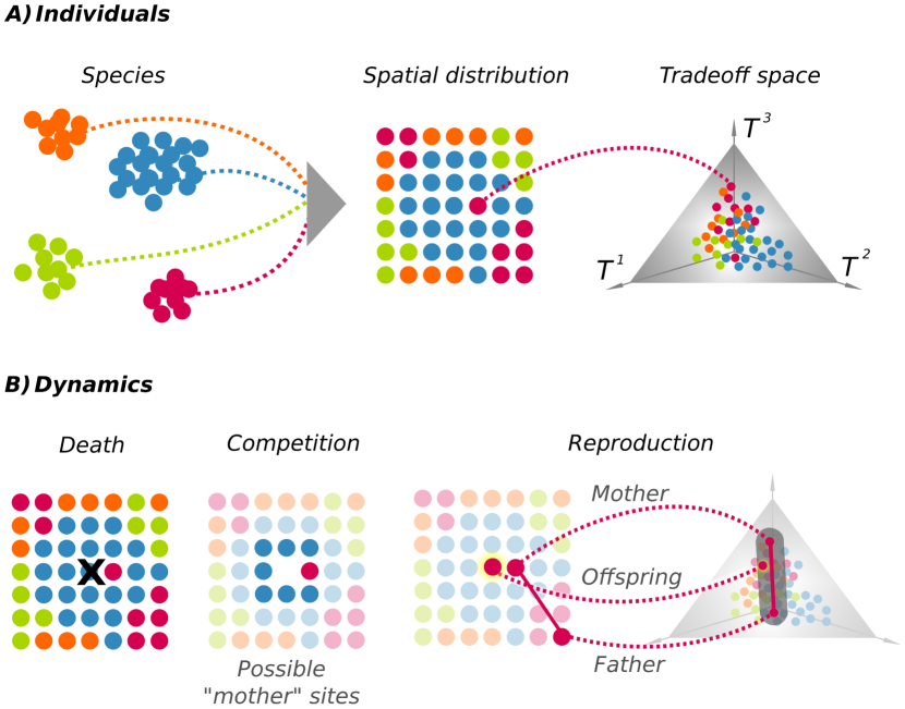
The traits of each single individual are determined by quantitative phenotypic values that can be regarded as the investment in specific functional organs. For instance, the traits could represent the proportion of biomass devoted to exploit soil nutrients (roots), light (leaves and stems), and to attract pollinators and capture pollen (flowers; see Fig. 1). We then assume a hard limit –constant across generations– to the amount of resources that can be devoted to generate the phenotype, i.e. it is impossible to increase all phenotypic values simultaneously. Thus each individual is constrained to make specific trade-offs in the way it exploits resources. Because similar values in the trade-off space entail comparable exploitation of the same resource (e.g., water, light or pollinators) similar individuals experience higher levels of competition, which translates into a lower fitness. This can be regarded as a frequency dependent selection mechanism providing an adaptive advantage to exceptional individuals, able to exploit available resources. Therefore, the ecological processes of competition, reproduction, and selection lead to evolutionary shifts in the distribution of phenotypic traits which feed back into community processes, giving rise to integrated eco-evolutionary dynamics.

Figure 1: (Color online) Sketch of the model. (A) Individuals of different species (different colors) compete for available resources in a physical space (two-dimensional square lattice), which is assumed to be saturated at all times. Each individual is equipped with a set of phenotypic traits that corresponds to a single point in the trade-off space. This is represented here (as a specific example) as an equilateral triangle (a “simplex” in mathematical terms) corresponding to the case of $3$ coordinates which add up to $1$ (e.g., fraction of the total biomass devoted to roots, leaves/stems and flowers, respectively (Tilman and Snell-Rood, 2014)). For instance, a point close to vertex $T^{1}$ exploits better the limiting resource $1$ (e.g. soil nutrients) than another one near vertex $T^{2}$, but is less efficient at exploiting resource $2$ (e.g. light) than this latter one (see Methods). (B) Individuals die after one timestep, giving rise to empty sites; each of these is occupied by an offspring from a “mother” within its local neighborhood (consisting of $8$ sites in the sketch for clarity, although we considered also a second shell of neighbors in the simulations, i.e. a kernel of 24 sites). The mother is randomly selected from the plants occupying this neighborhood in the previous generation, with a probability that decreases with the level of similarity/competition with its neighbors (see Methods). The implanted seed is assumed to have been fertilized by a conspecific “father” from any arbitrary random location, selected also with a competition-level dependent probability. The offspring inherits its phenotype from both parents; its traits can lie at any point (in the shaded region of the figure) nearby the the parental ones, allowing for some variation. For a given number of initial species $S$, two key parameters control the final outcome of the dynamics: $\beta$, characterizing the overall level of competition, and $\mu$, representing the variability of inherited traits. We fix most of the parameters in the model (lattice site, individuals within the competition/reproduction kernel, etc.) and study the dependence on $S$, $\beta$ and $\mu$.

2.2 Model construction

The basic components of the model are as follows (further details are deferred to the Methods section). We consider a community of individuals of $S$ different species, that are determined initially by mating barriers (i.e. a species is defined as a set of individuals that can produce fertile offspring (Coyne and Orr, 2004)). Each individual occupies a position in physical space (represented as a saturated square lattice) and is characterized by the label of the species to which it belongs and a set of intrinsic parameters (i.e. trait values), specifying its coordinates in the “trade-off space” as sketched in Fig. 1 (see also (Rulands et al., 2014; Tilman and Snell-Rood, 2014). All positions within the trade-off space are assumed to be equally favorable a priori. In what follows, we make a perfect identification between the trade-offs of a given individual and its phenotypic traits, which also determine the “niche” occupied by each individual. In principle, each individual, regardless of its species, can occupy any positition in the trade-off space. Positions near the center of the trade-off space (Fig. 1) correspond to phenotypes with similar use of the different resources (i.e., “generalists”), while individuals near the corners specialize in the exploitation of a given resource (“specialists”).

Individuals are subjected to the processes of birth, competition for resources, reproduction, descent with modification, and death. Individuals are assumed to undergo sexual reproduction, as in the experiments of (Zuppinger-Dingley et al., 2014) (implementations with asexual reproduction are discussed later); they are considered to be semelparous, so that after one simulation time step (i.e, a reproductive cycle) they all die and are replaced by a new generation. Importantly, demographic processes are strongly dependent on phenotypic values. In particular, the main niche-based hypothesis is that individual organisms with a better “performance” are more likely to reproduce than poorly performing ones. To quantify the notion of “performance”, we rely on classical concepts such as limiting similarity, competitive exclusion principle and niche overlap hypothesis limiting similarity, competitive exclusion principle and niche overlap hypothesis (May and Mac Arthur, 1972; Pianka, 1974), which posit that in order to avoid competition, similar species must differ in their phenotypes. More specifically, our model assumes that the performance of a given individual increases with its trait “complementarity” to its spatial neighbors (Pianka, 1974), as quantified by its averaged distance to them in trade-off space (see Methods); i.e. the larger the phenotypic similarity among neighbors, the stronger the competition, and the worse their performance. Although the performance of a given individual depends on its complementarity with its neighbors, the model is symmetric among species and phenotypes; performance is blind to species labels and does not depend on the specific location in the trade-off space.

The reproduction probability or performance of any given individual is mediated by a parameter $\beta$ which characterizes the global level of competitive stress in the environment (see Methods). In the limit of no competition, $\beta=0$, the dynamics become blind to phenotypic values and can be regarded as fully neutral, while in the opposite limit of extremely competitive environments, $\beta\rightarrow\infty$, niche effects are maximal and a relatively small enhancement of trait complementarity induces a huge competitive advantage. Finally, a mother selected as described in the competition process is assumed to be fertilized by a conspecific “father” in the population (interspecies hybridization is not considered here) which is also selected with the same reproduction probability function based on its performance. The offspring inherits its traits from both parents, with admixture and some degree of variation $\mu$ (see Fig. 1 and Methods). This process is iterated for all lattice sites and for an arbitrarily large number of reproductive cycles, resulting in a redistribution of species both in physical and in trade-off space. Species can possibly go extinct as a consequence of the dynamics. In this version of the model, speciation is not considered, though it could be easily implemented by establishing a dependence of mating on phenotypic similarity, making reproduction between sufficiently different individuals impossible (De Aguiar et al., 2009).

2.3 Computational results

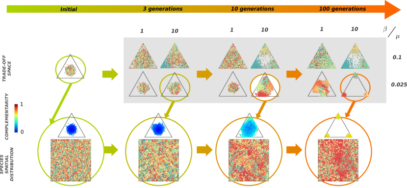
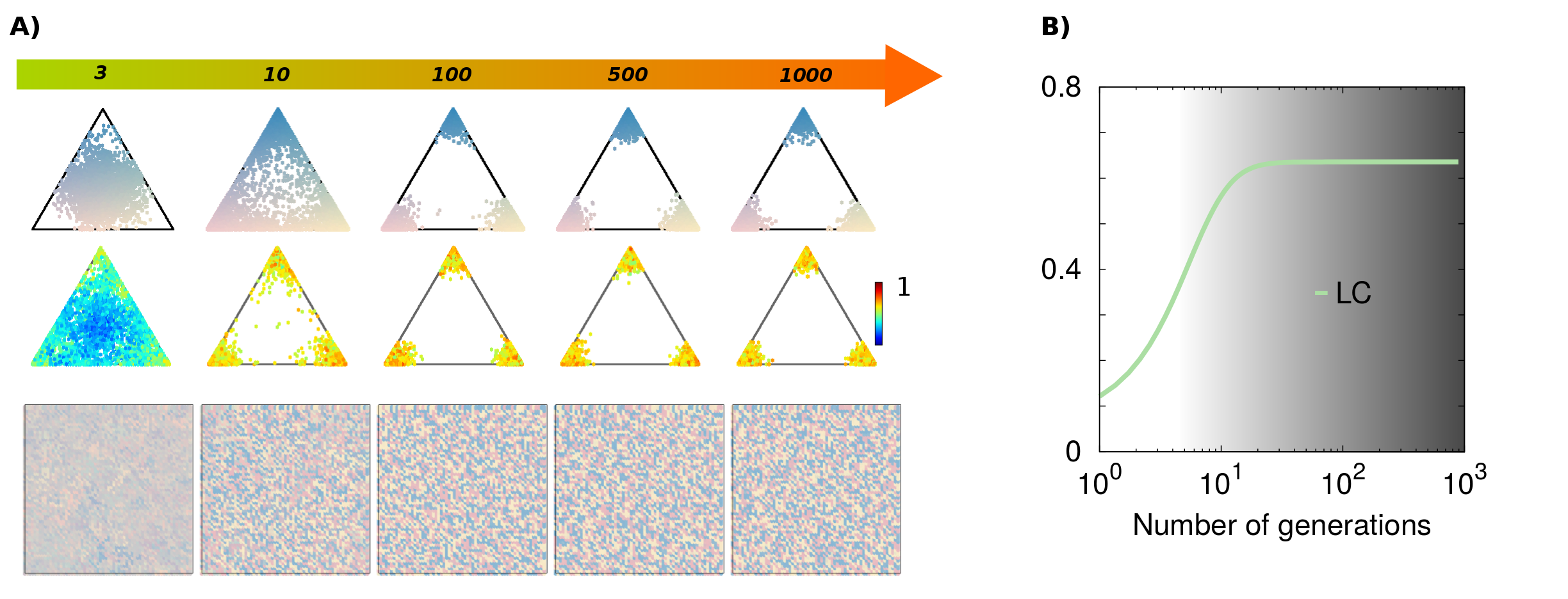
Simulations are started with individuals of $S$ different species (e.g. $S=16$) randomly distributed in space. In the initial conditions, the traits of all individuals are a sample from a common Gaussian distribution centered around the center of the simplex (note that as shown in the S5 Appendix in Supporting Information, results do not depend on the particular choice of initial conditions). Statistical patterns emerging from the eco-evolutionary dynamics described above are analyzed as a function of the number of generations and as a function of the number of species $S$, for different values of the two free parameters: the overall level of competition $\beta$ and the variability of inherited traits $\mu$. Results are illustrated in Fig. 2 showing (i) phenotypic diagrams (top row) specifying the position of each single individual and its species in the trade-off space for different parameter values and evolutionary times (ii); values of complementarity for all individuals (central row) in the trade-off space, and (iii) the spatial distribution of individuals and species (bottom row). Finally, several biodiversity indices are reported in Fig. 3.

Figure 2: (Color online) Illustration of the emergence of rapid phenotypic diversification for a computational system of size $64\times 64$ and $16$ species (labeled with different colors). (Top). Phenotypic diagrams measured at different evolution stages ($1$, $3$, $10$ and $100$ generations, respectively) for different values of the two parameters: level of competition $\beta$ ($1$ for the case of low competition and $10$ for strong competition) and variation in inherited traits $\mu$ ($0.1$ for large variation and $0.025$ for small variation). In all cases, phenotypic differentiation among species is evident even after only $10$ generations. In the long term ($100$ generations) species diversification and specialization is most evident for small $\mu$ and large $\beta$; in this last case, different species (colors) can coexist for large times in the same region/corner of trade-off space. (Central). Complementarity diagrams representing the values of averaged local complementarity for all individuals of any species for small $\mu$ ($0.025$) and large $\beta$ ($10$). Individuals with small complementarity (i.e. under strong competition with neighbors) disappear in the evolutionary process, while communities with high degrees of local complementarity are rapidly selected. (Bottom). Spatial distribution of species for different number of generations. As a result of the eco-evolutionary dynamics, anti-correlated patterns –in which neighboring plants tend to be different– emerge (note that colors represent species assignment and do not reflect phenotypic values)

Figure 3: (Color online) Measurements of different biodiversity indices. (A) Phenotypic distances among species grow systematically during the eco-evolutionary process, reflecting a clear tendency towards species differentiation (same sets of parameter values as in Fig. 2, $S=16$). Differentiation is faster for relatively small values of trait variability $\mu$ and large values of the competitive stress $\beta$. (B) Phenotypic differentiation among and within species. While interspecies distances grow in time for all values of $S$ and converge to similar values on the long term, intraspecific phenotypic variability is much larger on the long term for monocultures than for biodiverse mixtures. (C) Phenotypic similarity among close neighbors. Moran’s index ($I$) for $\beta=10$ and different values of $S$ as well as for $\beta=0$ and for a random distribution (i.e. in the absence of spatial interactions). The value of $I$ tends to $0$ for random distributions, is positive for $\beta=0$, and tends to small negative values for $\beta\neq 0$. Whenever competition depends on the phenotypic values (i.e., $\beta>0$) the system avoids close cohabitation of individuals of the same species. This negative spatial autocorrelation results in $I<0$; in all cases, $\mu=0.025$. (D) Averaged local and relative complementarity in the community increase with time and reach larger values for more biodiverse communities. The phenotypic differentiation among individuals is greater both among close neighbors and at the global scale as the number os species $S$ increases. In all plots, parameters are $L=64$ and, unless it is specified, $\beta=10$ and $\mu=0.025$; curves are averaged over at least $10^{3}$ runs; shaded light grey areas stand for times during which extinction tends to occur causing $S$ to decrease (see S10 Appendix in Supporting Information for details), while in dark grey ones the system tend to stabilize at a given final number of species.

2.3.1 Species differentiation

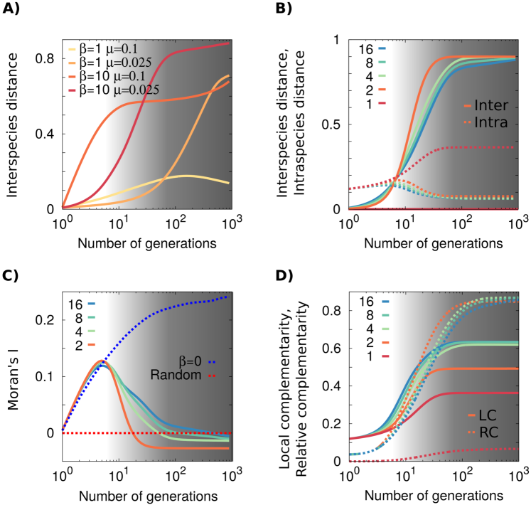
As illustrated in Fig. 2 (shaded area), different distributions of individuals in the trade-off space appear depending on the specific values of $\beta$ and $\mu$. Visual inspection reveals the emergence of rapid phenotypic differentiation, i.e. segregation of colors in trade-off space after a few (e.g. $10$) reproductive cycles. The segregation is much more pronounced for relatively small variability (e.g. $\mu=0.025$) and large competitive stress (e.g. $\beta=10$). This is quantified (see Fig. 3A) by the average interspecies distance (see Methods), whose specific shape depends on parameter values. As shown in Fig. 3B, the fastest growth is obtained for $S=2$, but the curves converge to a constant value (mostly independent of $S$) after a sufficiently large number of generations. Moreover, as shown in the central row of Fig. 2 the complementarity –averaged over all individuals in the community (see Methods)– also grows during the course of evolution (i.e. colors shift from blue to yellowish). Observe in Fig. 2. that, for asymptotically large evolutionary times, there is a tendency for all species to cluster around the corners of the trade-off space, suggesting that the optimal solution to the problem of minimizing the competition with neighbors corresponds to communities with highly specialized species. This specialization does not occur in monocultures ($S=1$), as sexual mating pulls the species together and avoids significant phenotypic segregation.

2.3.2 Emergence of local anti-correlations

The high level of phenotypic specialization observed after large evolutionary times for large competition stress and small variability, might seem in contradiction with the overall tendency to niche differentiation. In other words, most of the trade-off space becomes empty in this case, while individuals aggregate at the (highly populated) corners. The answer to this apparent conundrum is that similarly specialized individuals have a statistical tendency to avoid being spatial neighbors. Indeed, as qualitatively illustrated in the lowest right panel of Fig. 2, extreme specialization is accompanied by a tendency to diminish spatial clustering, i.e. to create spatial anti-correlations within each species. This tendency –which stems from intraspecific competition and opposes to the demographic tendency of similar individual to cluster in space– is quantitatively reflected by negative values of Moran’s index $I$ (see Fig. 3C and Methods). Note also that $I$ and thus the spacial distribution of species, is radically different in the presence and in the absence of competition (i.e. for $\beta\neq 0$ and $\beta=0$, respectively) as can be seen in Fig. 3C. In the absence of competition, species are distributed randomly forming aggregated spatial clusters without competition-induced local anti-correlations.

2.3.3 Intraspecific diversity

This quantity is defined as the mean “complementarity” among all pairs of conspecific individuals in the community, and illustrates the level of phenotypic diversity within species. As shown in Fig. 3B, the intraspecific diversity is much larger for monocultures. In monocultures, neighbors are obviously conspecific and the only available mechanism to reduce overall competition is to increase intraspecific diversity. Therefore, as a general result, monocultures tend to enhance their intraspecific phenotypic distances, while biodiverse communities tend to enhance phenotypic differentiation among species but result in more similar conspecifics.

2.3.4 Local complementarity

Fig. 3D shows the evolution of the mean complementarity of individuals respect to its spatial neighbors. This averaged local complementarity (LC) controls the dynamics and the actual reduction in the level of competition for a given spatial distribution, and is much larger for mixtures than for monocultures (it grows monotonously with $S$ and saturates at a maximal value).

2.3.5 Global complementarity

Similarly, we can measure “global” complementarity (GC), i.e. the average phenotypic distance among all individuals in the experiment, regardless of their spatial coordinates, after a given number of generations. Additionally, we measured $\mathrm{GC}_{\mathrm{intra}}$ (resp. $\mathrm{GC}_{\mathrm{inter}}$) which is $\mathrm{GC}$ averaged only over individuals of the same (resp. different) species (see Methods). In Fig. 3D we present results for the relative complementarity $\mathrm{RC}=\mathrm{GC}_{\mathrm{inter}}-\mathrm{GC}_{\mathrm{intra}}$, which is a measure of the averaged difference in the level of competition between randomly sampled non-conspecific and conspecific individuals, respectively. Observe that the RC is larger for mixtures than for monocultures, $\mathrm{RC}(S>1)>\mathrm{RC}(S=1)$, and that it grows faster in time for smaller values of $S$ (e.g. $S=2$), but reaches almost equal constant values after a sufficiently large number of generations.

2.3.6 Emergent neutrality

As illustrated in Fig. 2, different species with very similar trait values can coexist (e.g. yellow and orange species at the right corner of the phenotypic diagram for $\mu=0.025$ and $\beta=10$ in Fig. 2) even after many generations. Such a coexistence emerges spontaneously and although it is transitory it can last for arbitrarily long times provided that the system size is sufficiently large. From an ecological point of view, these species can be regarded as functionally equivalent as they occupy the same niche region (see S6 Appendix in the Supporting Information for a detailed analysis of the stability and coexistence time of such species).

2.3.7 Model variants

To investigate the generality of our findings, we also explored whether the main conclusions are robust against some constraints of the implementation. We briefly explain the variants we took into account below. i) Non-symmetrical phenotypic trade-offs: as a first step, we assumed that not all positions in the trade-off space are equally rewarding a priori: individuals in certain regions of the trade-off space have larger reproduction probabilities than others. Non-symmetrical trade-offs lead to very similar results as above, confirming the robustness of our conclusions (see S7 Appendix in Supporting Information). ii) Asexual reproduction: as shown in S8 Appendix in Supporting Information, for communities of individuals able to reproduce asexually (i.e. assuming transmission of traits only from the mother) the outcome of the model is different: individuals tend to diversify, but such diversification occurs even within species (i.e. intra-specific diversification is much larger than in the sexual case); in other words, since there is no admixing of the phenotypic traits through reproduction, diversification occurs within maternal lineages, rather than at the species level. iii) Long-distance dispersal and competition: we also studied the case in which dispersal and competition are long-distance processes and affect the whole community and not only close neighbors; as shown in S3 Appendix in Supporting Information the phenomenology reported above remains quite similar, even if in this well-mixed case the co-existence of phenotypically-equivalent species is less likely (owing to the lack of spatial separation). iv) Effect of the competition kernel: the specific form of the competition kernel can play a crucial role in the formation of species clusters in phenotypic space (Geritz et al., 1999; Adler and Mosquera, 2000; Pigolotti et al., 2007; Ramos et al., 2008; Hernández-García et al., 2009; Barabás et al., 2013; Lampert and Hastings, 2014); in the S9 Appendix of the Supporting Information we explore different kernel functions and show that our results are robust against changes in the mathematical expression of competition.

3 Discussion

In the present paper, we have developed a parsimonious modeling approach to integrate important ecological and evolutionary processes. In particular, we focused on understanding rapid phenotypic diversification observed in complex biological communities of plants such as those recently reported by Zuppinger-Dingley et al. in long-term field experiments (Zuppinger-Dingley et al., 2014; Tilman and Snell-Rood, 2014).

Our model blends standard community processes, such as reproduction, competition or death, with evolutionary change (e.g., descent with modification); i.e. community and evolutionary dynamics are coupled together, feeding back into each other. Over the last decades, attempts to integrate ecological and evolutionary dynamics have been the goal of many studies (see e.g. (Dieckmann et al., 1995; Dieckmann and Law, 1996; Law et al., 1997; Thompson, 1998; Dieckmann and Doebeli, 1999; Doebeli and Dieckmann, 2000, 2003; Schluter, 2000; Loeuille and Loreau, 2004; Carroll et al., 2007; Strauss et al., 2008; Fussmann et al., 2007b; DeAngelis and Mooij, 2005; Champagnat et al., 2006; De Aguiar et al., 2009; Hanski, 2012; Doebeli, 2011; Cremer et al., 2011; Rulands et al., 2014)). In particular, a basic algorithm for modeling eco-evolutionary dynamics as a stochastic process of birth with mutation, interaction, and death was proposed in (Dieckmann et al., 1995) and much work has been developed afterwards to incorporate elements such as spatial effects and different types of interspecies interactions (Doebeli and Dieckmann, 2003).

Rather than providing a radically different framework, our model constitutes a blend of other modeling approaches in the literature of eco-evolutionary processes, and in fact it shares many ingredients with other precedent works, specially with the theory of adaptive dynamics (Doebeli, 2011; Fussmann et al., 2007a). For instance, Gravel et al. (Gravel et al., 2006a) also considered a spatially-explicit individual-based model with trait-dependent competition. However, our work has been specifically devised to shed light on the experimental findings of Zuppinger et al.(Zuppinger-Dingley et al., 2014), and puts the emphasis on communities with arbitrarily large number of species, while usually the focus is on the (co-)evolution of pairs of species (e.g. predator-prey, host-parasite, etc.) or speciation/radiation of individual species. Finally, our modelling approach is sufficiently general as to be flexible to be adapted to other situations with slightly different ingredients. We explored some of these possible extensions in some Appendices (S3,S4,S7,S8,S9) in Supporting Information (e.g long-distance dispersal, asexual reproduction, etc.), but other studies can be built upon the work laid here in a relatively simple way.

The present model relies on a number of specific assumptions, two of which are essential in that they couple community and evolutionary dynamics: i.e. (i) demographic processes are controlled by competition for resources which is mediated by phenotypic traits and (ii) successful individuals are more likely to transmit their phenotypes to the next generation with some degree of variation. These two ingredients are critical for the emerging phenomenology. For instance, in the absence of competition (i.e. $\beta=0$) reproduction probabilities are identical for all individuals, implying that the model becomes neutral, and the evolutionary force leading to species differentiation vanishes (see S4 Appendices in Supporting Information). On the other hand, variation in inherited traits is necessary to allow for the emergence of slightly different new phenotypes and the emergence of drifts in trade-off-space. Although these constraints might be regarded as limiting, we deem them biologically realistic and do not think they hamper the predictive power of our model. Most of the remaining ingredients, such as the existence of a saturated landscape, semelparity (i.e. non-overlapping generations), the specific form in which we implemented initial conditions, competition, dispersion, selection, inheritance linked to phenotypic characters rather than to a genotypic codification, etc. can be modified without substantially affecting the results. This flexibility could make the description of other type of communities possible with minimal model variations. Similarly, the model could be extended to incorporate phenotype-dependent reproductive barriers (and thus speciation) and the possibility of interspecies hybridization by making reproduction a function of phenotypic distance and relaxing its dependency on species labels.

In addition to rapid phenotypic diversification, the experiments of Zuppinger et al. found an enhancement of the overall productivity in mixtures of diverse plants with respect to monocultures of the same plants (Zuppinger-Dingley et al., 2014). Our model cannot be used to directly quantify such “biodiversity effects” (Loreau and Hector, 2001), as we assume a fully saturated landscape and there is no variable that accounts for total biomass production. However, in principle, under the hypothesis that larger trait complementarities correlate with greater resource capture and biomass production, the observed increase of relative complementarity in mixtures (see Fig. 3) could be used as a proxy for biodiversity effects. Observe, nonetheless, that the previous assumption might by wrong (or incomplete) as productivity can be profoundly affected by other factors such as, for instance, positive interactions between similar species, not modeled here, and more sophisticated approaches –see (Hooper et al., 2005; Duffy et al., 2007; Cardinale et al., 2009; Reiss et al., 2009; Grace et al., 2016)– are necessary to validate this hypothesis. In the future we plan to modify our model to represent non-saturated landscapes and more detailed ecological dynamics, allowing for explicit analyses of biodiversity-productivity relationships.

Beyond explaining most of the empirical observations in (Zuppinger-Dingley et al., 2014), our model leads to some far-reaching predictions (some of them already shared by existing theories); one of the most remarkable ones is that optimal exploitation of resources comes about when the full community evolves into a reduced number of highly specialized species –the exact number depending on the dimensions of the trade-off space– that coexist in highly dispersed and intermixed populations. Such specialization might be unrealistic in the case in which all traits in trade-off space are essential for survival, and thus the convergence toward perfect specialization is capped. In any case, this result is congruent with the niche dimension hypothesis (Hutchinson, 1957), that postulates that a greater diversity of niches entails a greater diversity of species, i.e. a larger number of limiting factors (and thus of possible trade-offs) leads to richer communities (Harpole and Tilman, 2007). However, this outcome might be affected by perturbations (migration, environmental variability, etc) which could be easily implemented in our model, and could prevent real communities from reaching the asymptotic steady state predicted here. It is also noteworthy that the resulting highly specialized species can be phenotypically equivalent, and a set of them can occupy almost identical locations in the trade-off space. Such species equivalence appears spontaneously, and supports the views expressed by other authors that “emergent neutrality” is a property of many ecosystems (Allan et al., 2013; Scheffer and van Nes, 2006b; Barabás et al., 2012). In future work we will explore the possibility of phase transitions separating an ecological regime based on the coexistence of multiple highly specialized species from an ecosystem dominated by generalists and the conditions under which each regime emerges.

Beyond phenotype-dependent mating, upcoming studies will extend our approach to address communities where collective diversification phenomena based on both competition and cooperation are known to emerge (see e.g. (Cordero and Polz, 2014)), as well as investigate the evolution of communities with distinct types of interacting species such as plant-pollinator mutualistic networks. This research will hopefully complement the existing literature and help highlighting the universal and entangled nature of eco-evolutionary processes.

4 Methods

4.1 Model implementation

We implemented computer simulations in which each individual plant, $i$, is fully characterized by (see also Fig. 1): (i) a label identifying its species, (ii) its coordinates in the physical space, and (iii) a set of real numbers specifying its phenotypic traits. In these simulations, time can be implemented either as discrete/synchronous updating or continuous/sequential updating without significantly altering the results. Species–, we consider a fixed number of species, labeled from $1$ to $S$; while the emergence of new species is not considered here, some of them may become extinct along the course of evolution. Physical space– We consider a two-dimensional homogeneous physical space described by a $L\times L$ square lattice, assumed to be saturated at all times, in which the neighborhood of each individuals is determined by the closest $K$ sites (in our simulations, we took $L=64$ and $K=24$). Phenotypic traits and trade-off space– As energy and resources are limited, each individual plant needs to make specific choices/trade-offs on how to allocate different functions. The way we implement the “trade-off space” is inspired in the field of multi-constraint (non-parametric) optimization that it is called Pareto optimal front/surface (Miettinen, 1999); it includes the set of possible solutions such that none of the functions can be improved without degrading some other. Thus, the phenotype of any individual can be represented as a trade-off equilibrium, a point in this space and encapsulated in a set of real numbers $\mathbf{T}=(T^{1},T^{2},...,T^{n})$ (all of them in the interval $[0,1]$), such that $\sum_{k=1}^{n}T^{k}=1$ where $n$ is the number of trade-offs (see Fig. 1 and (Tilman and Snell-Rood, 2014)). All positions within the trade-off space are equivalent a priori, although this requirement can be relaxed. Competition for resources– The trait “complementarity” between two individuals $i$ and $j$ is quantified as their distance in the trade-off space: $c_{ij}=\sum_{k=1}^{n}|T^{k}(i)-T^{k}(j)|/n$, which does not depend on species labels. The averaged complementarity, (or simply “complementarity”) over all the neighbors $j$ of individual $i$ is $C_{i}=\sum_{j\in n.n.(i)}c_{ij}/K$. Complementarity-based dynamics– Each timestep, every individual is removed from the population; the resulting vacant site $i$ is replaced by an offspring of a potential mother plant $j$ which is selected from the list of $K$ local neighbors of the vacant site with a given probability $P_{\mathrm{mother}}(j)$. This probability controls the dynamical process; we assume it to increase as the mother’s trait complementarity $C_{j}$ increases (i.e. as its effective competitive stress diminishes): $P_{\mathrm{mother}}(j)={e^{\beta C_{j}}}/{\sum_{j^{\prime}\in n.n.(i)}e^{\beta C_{j^{\prime}}}}~{}$, where the sum runs over the set of $K$ neighbors of $i$; $e^{\beta C_{j}}$ is the “performance” of individual $j$ and $\beta$ is a tunable “competition parameter” controlling the overall level of competitive stress in the community. Once the mother has been selected, the father is randomly chosen from all its conspecific individuals $l$ in the community, with a probability proportional to their performance, ${e^{\beta C_{l}}}$. In other words, individuals with lower competition pressure are more likely to sire descendants both as females and as males. Inheritance, admixture and variation of phenotypes– The traits of each single offspring are a stochastic interpolation of those of both parents with the possibility of variation: $T^{k}_{\mathrm{new}}=\eta T^{k}_{\mathrm{mother}}+(1-\eta)T^{k}_{\mathrm{father}}+\xi^{k}$, for $k=1,...,n$, where $\eta$ is a random variable (uniformly distributed in $[0,1]$) allowing for different levels of admixture for each offspring, and $\xi_{k}$ are (Gaussian) zero-mean random variables with standard deviation $\mu$, a key parameter that characterizes the variability of inherited traits. To preserve the overall constraints $T^{k}\in[0,1]$ and $\sum_{k}T^{k}=1$, mutations are generated as $\xi^{k}=(r^{k}-r^{k+1})$, where $\{r^{1}=r^{n+1},...,r^{n}\}$ are independent Gaussian random variables with zero-mean and standard deviation $\mu/\sqrt{2}$; in the rare case that $T^{k}_{\mathrm{new}}<0$ (resp. $>1$), we set it to $0$ (resp. to $1$) and added the truncated difference to another random trait.

4.2 Biodiversity indices

The centroid of species $s$ is ${\bf{B}}(s)=\{B^{1}(s),...,B^{n}(s)\}$, with $B^{k}(s)=\sum_{i}T^{k}(i)/n_{s}$ for each trait $k$, where $i$ runs over the $n_{s}$ individuals of species $s$. Interspecies distance: is the distance between the centroids of two different species $s$ and $s^{\prime}$ in the trade-off space $d_{s,s^{\prime}}=\sum_{k}|B^{k}(s)-B^{k}(s^{\prime})|/n$, averaged over all surviving species. Intraspecific distance is the average distance in trade-off space between all pairs of individuals of a given species $s$, $d_{s}=\sum_{i,j\in s}c_{ij}/n_{s}(n_{s}-1)$ averaged over all surviving species. Local complementarity is the the mean complementarity of individuals to their spatial neighbors, $\mathrm{LC}=\sum_{i}(\sum_{j\in n.n.(i)}c_{ij}/K)/N$ where $N$ is the total number of individuals and $K$ is the number of local neighbors. Global complementarity is the complementarity averaged over all pairs of individuals regardless of their relative positions in physical space, $\mathrm{GC}=\sum_{i,j\neq i}c_{ij}/(N(N-1))$. Similarly $\mathrm{GC}_{\mathrm{inter}}$ is the averaged complementarity between individuals of different species and $\mathrm{GC}_{\mathrm{intra}}$ is the averaged complementarity between conspecific individuals. In the case of monocultures, $\mathrm{GC}_{\mathrm{inter}}(S=1)$ is measured from two different/independent realizations. Relative complementarity, $\mathrm{RC}=\mathrm{GC}_{\mathrm{inter}}-\mathrm{GC}_{\mathrm{intra}}$, is a measure of the averaged difference in the level of competition between randomly sampled conspecific and non-conspecific individuals. Moran’s index: is a measure of spatial correlations between neighbors; it is negative when neighbors tend to belong to different species (see S2 Appendix in Supporting Information).

5 Acknowledgements

We acknowledge support from the Spanish MINECO project FIS2013-43201-P. RRC is supported by the Talentia Program (Junta de Andalucía / EC-FP7 COFUND – Grant Agreement 267226).

Supporting Information

S1. Local and global trait complementarities

We distinguish three different measures regarding averaged complementarities (see the sketches in Fig. 4): i) Local complementarity (LC), defined as the mean phenotypic distance between an individual and its spatial neighbors; ii) Intraspecific global complementarity (GC_intra), defined as the mean phenotypic distance between all pairs of individuals within the same species (and then averaged over species); and, additionally, iii) Interspecific global complementarity (GC_inter), corresponding to the the mean phenotypic distance between all pairs of individuals consisting of individuals of two different species (averaged over all species). While local measurements capture the effect of spatial correlations, global ones are useful to characterize the evolution of the whole community in trade-off space. In analogy with the experimental setup of Zuppinger-Dingley et al. (Zuppinger-Dingley et al., 2014), we performed computer simulations using both monocultures and mixtures. For the case of monocultures, GC_inter was estimated taking individuals coming from two independent realizations of the simulations. Zuppinger et al. gathered seeds from surrounding populations and grew them together in their experimental set-up. This removed any cumulative, trans-generational effect of spatial correlations. In this way, GC measurements (Fig. 4 B) constitute better proxies (as compared to LC) to contrast our results with global community (biodiversity) effects in (Zuppinger-Dingley et al., 2014).

Figure 4: (Color online) complementarity measurements:

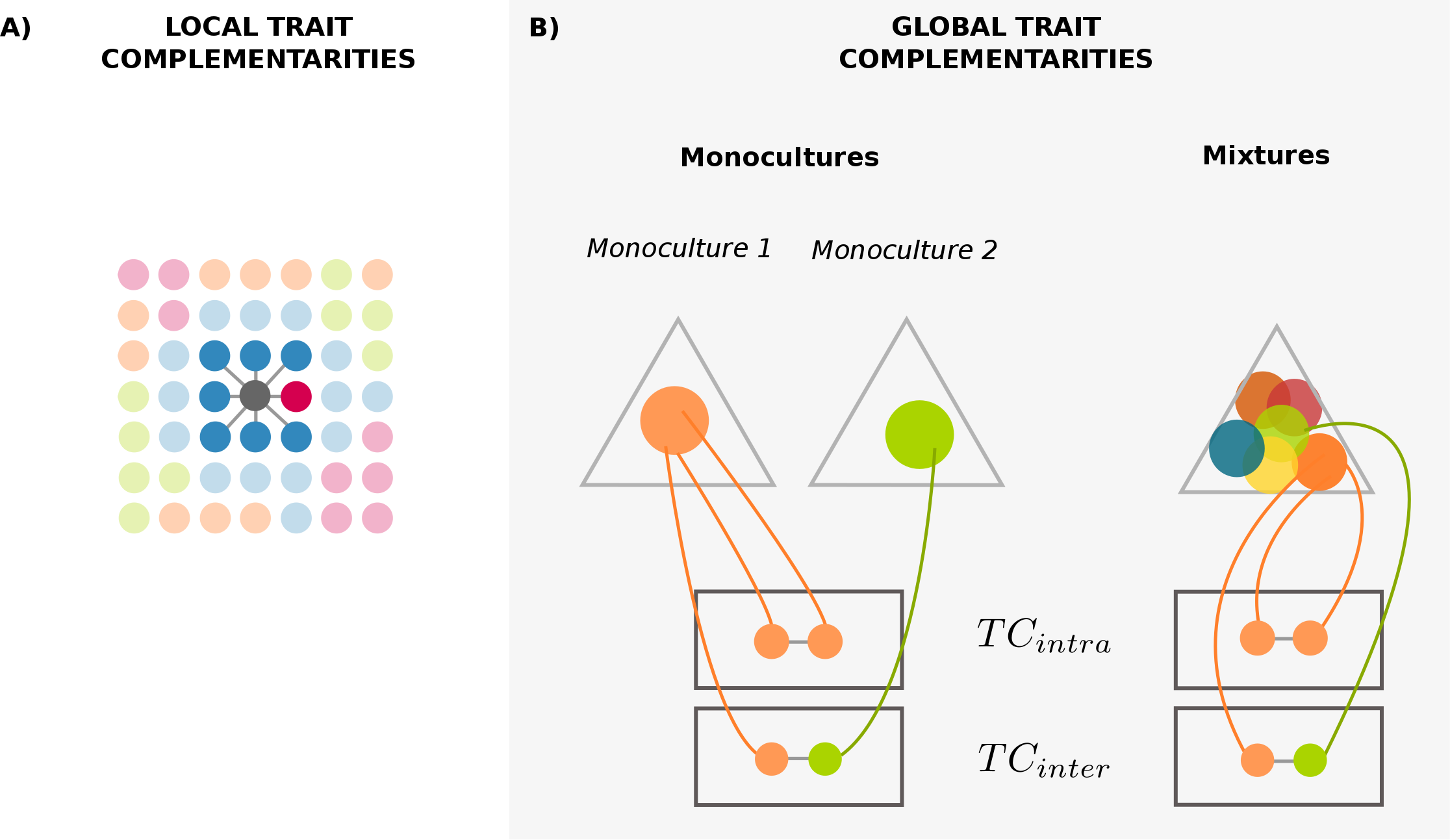
A) Local complementarity (i.e. mean phenotypic distance between spatially close neighbors) reveals the effect of spatial correlations; B) Intraspecific and interspecific global complementarities (i.e. mean phenotypic distance between individuals of the same and of different species, respectively, regardless of their spatial location). In all cases, we performed computer simulations using monocultures and mixtures.

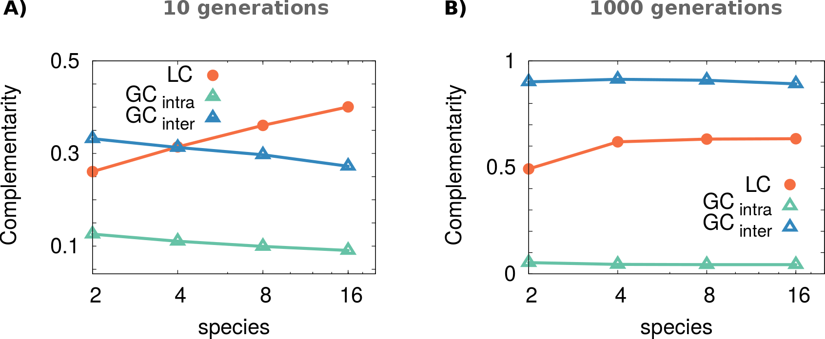
Complementing the results presented in Fig. 3 of the main text, Fig. 5 shows measurements for LC and GC_intra/inter for different initial number of species $S$ after $10$ and $1000$ generations. We observe that, even though complementarities become almost independent of $S$ at $t=1000$ (due to the extinction of some species), transient measurements at $t=10$ clearly show that communities with fewer species exhibit higher values of GC and, consequently, reach the stationary state faster. Biodiversity delays the process because several species simultaneously compete for empty niches. On the other hand, LC is inversely correlated with $S$, i.e., individuals tend to be more phenotypically similar to ás in less biodiverse communities.

Figure 5: (Color online) Local and global complementarities after A) $10$ and B) $1000$ reproductive cycles, plotted as a function of the initial number of species $S$ in the community. Parameter values (see main text): system size $L=64$, competition $\beta=10$ and variability $\mu=0.025$.

S2. Moran index

The Moran’s index (Moran, 1950) quantifies the likelihood of an individual to be surrounded by individuals of the same species. When Moran’s index is negative, individuals are less likely to be close to their co-specifics than what would be expected by pure chance, while positive values indicate spatial clustering of species. Mathematically, given a species $s$ we compute its Moran’s index $I_{s}$ as

$$I_{s}=\frac{\sum_{i\in s}\sum_{j\in n.n.(i)}(X_{s}^{i}-\bar{X}_{s})(X_{s}^{j}-\bar{X}_{s})}{K\sum_{i\in s}(X_{s}^{i}-\bar{X}_{s})^{2}},$$ (1)

where $K$ is the number of local neighbors (kernel size), and $X_{s}^{i}$ is a variable such that $X_{s}^{i}=1$ when the specie of $i$ is equal to $s$ and $X_{s}^{i}=0$ if it is different, with $\bar{X}_{s}$ the density of individuals of species $s$. Finally, we obtain the total index averaging over species, $I=\sum_{i=1}^{S}I_{s}/S$. As a result, positive, zero, and negative values of $I$ correspond to positive spatial correlation, random, and anti-correlation of species, respectively.

S3. Long-distance dispersal and competition

We have also studied well mixed (or “fully connected” ) communities, in which i) there is frequent long-distance dispersal (so that both progenitors of the new offspring can be located at any site in space) and, additionally, ii) each individual competes with the rest of the community, i.e. all individuals behave as nearest neighbors.

As illustrated in Fig. 6, all the previously reported phenomenology is still present in this ideal mean-field scenario. As a matter of fact, phenotypic differentiation seems to occur faster than when spatial distribution is conditioned by local dispersal (see Fig. 3). In other words, long-distance dispersal and global competition drive evolution faster than local dynamics. This is a consequence of enhanced competition, which increases the relative fitness of better performing individuals. Another important difference is that, under mean field conditions, equivalent taxa cannot occupy different spatial locations and are forced to compete with each other. Consequently, coexistence of species with similar traits is much less likely than in spatially-explicit communities.

Figure 6: (Color online) Evolution of the community with long-distance dispersal and global competition (i.e. well-mixed or mean-field dynamics). A) Tradeoff space and complementarity measured at different generations. B) Inter and intra-specific distances, and local complementarity and relative complementarity (RC= GC_inter-GC_intra) in time. Parameters: $L=64$, $S=16$, $\beta=10$, $\mu=0.025$.

S4. Comparison with neutral theory ($\beta=0$)

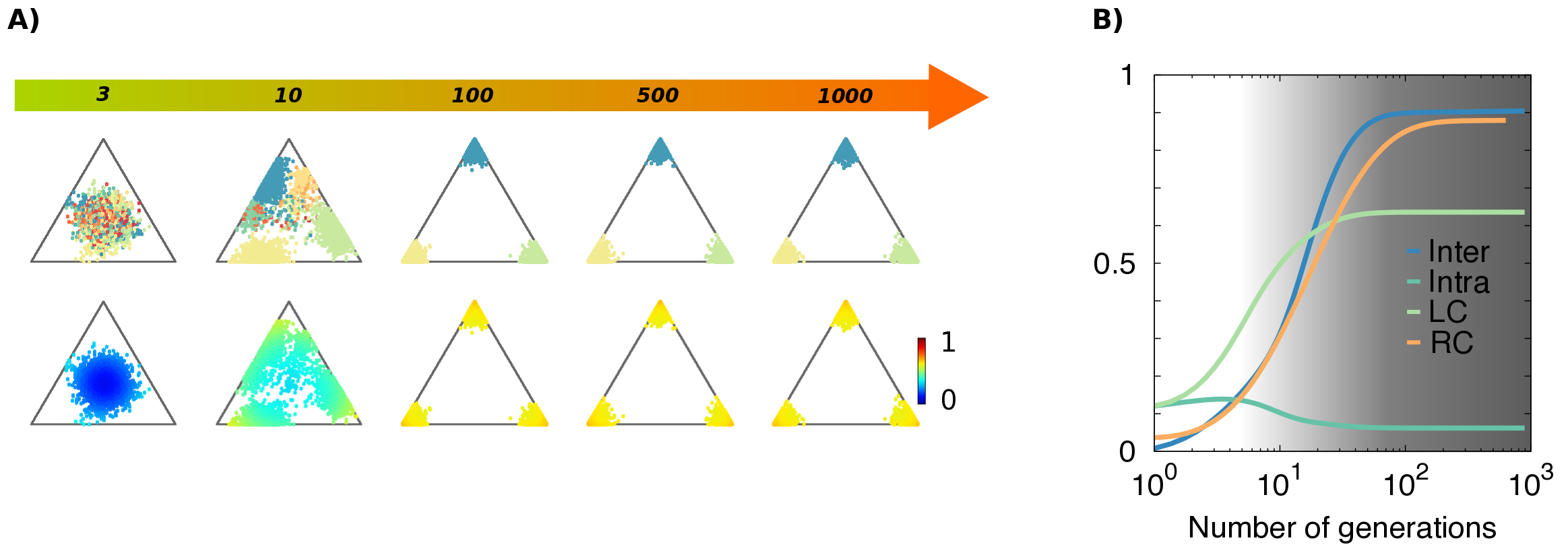
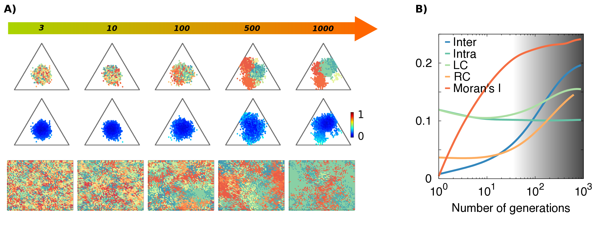
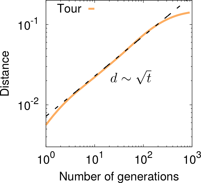
In the limit of no competition, $\beta=0$, our model equates to neutral-theory (Hubbell, 2001) in which reproduction probabilities become independent of individual phenotypes. Fig. 7 reports computational results for this case, illustrating the emergence of a very different scenario with respect to the non-neutral case. Sexual reproduction still pulls species together so they aggregate in the trade-off space, but their centroids describe slow and independent random walks instead of being controlled by a relatively fast separating drift (see Fig. 8). This phenomenology is caused by the lack of an effective force pushing species away; indeed segregated species can become closer after some generations, but on average there is only random drift allowing them to slowly diversify, so they cannot account for the empirical observations in (Zuppinger-Dingley et al., 2014). Similarly, relative complementarities (which in the absence of competition can be regarded as the averaged difference in the level of phenotypic similarity between randomly sampled non-conspecific and conspecific individuals) start to grow later and reach low values,

Figure 7: (Color online) Neutral dynamics ($\beta=0$), implying that all individuals have the same probability of reproduction independently of their species assignment and phenotype. A) Plots in the trade-off space illustrate that species hardly segregate in short time scales. In the physical space, local dispersal leads the the system to be clustered, i.e. positively auto-correlated rather than anti-correlated. B) Different measures illustrate that rapid evolutionary changes are much harder to observe in the neutral scenario. In particular, local complementarity (LC) and relative complementarity increase at a much slower pace. The increase in the Moran’s index confirms that the system remains positively correlated (as usually is the case in neutral models) Parameters have been set to $L=64$, $S=16$ and $\mu=0.025$.

Figure 8: (Color online) Species diffuse in the trade-off space under neutral dynamics ($\beta=0$): The plot shows average distance between species centroids and the central point of the phenotypic space (i.e. the position of all species centroids at $t=0$) as a function of time. Mutations cause a random movement of species centroids in the phenotypic space, as shown by the $0.5$ slope in double logarithmic scale, characteristic of diffusive processes. Parameter values are set as in Fig. 8.

S5. Initial phenotypic traits

In the main text, initial conditions are given by randomly sampling the value of each individual phenotypic trait from a single distribution (Gaussian around the center of the phenotypic space), independently of species labels. After some generations, we observe that competition causes species to segregate in phenotypic space.

Although the most widely accepted definitions of species are based exclusively on the role of mating barriers, individuals belonging to the same species tend to share common trait values. In this appendix, we approximate this kind of scenario and test the robustness of our results running simulations with partial clustering of species in phenotypic space. For this, we sampled individual traits from equal amplitude Gaussian distributions centered around different (randomly chosen) species-dependent points of the phenotypic space (see initial top panel in Fig. 9).

As illustrated in Fig. 9, species diversify sooner in phenotypic space (initial values for inter- and intra-specific distances are higher than in the case described in the main text) but after this transient difference asymptotic results remain essentially unchanged.

Figure 9: (Color online) Simulations under initial phenotypic segregation of species. Individual traits are initially sampled from different species-dependent Gaussian distributions. Each of these Gaussians have a standard deviation equal to 0.05 and a mean value randomly selected from another Gaussian (with the same amplitude 0.05) centered at the triangle barycenter. A) From top to bottom: Tradeoff values, trait complementarities, and spatial distributions at different generations. B) Evolution of the inter and intra-specific distances, local and relative complementarity and Moran’s Index. Parameters: $L=64,S=16,\beta=10,\mu=0.025$.

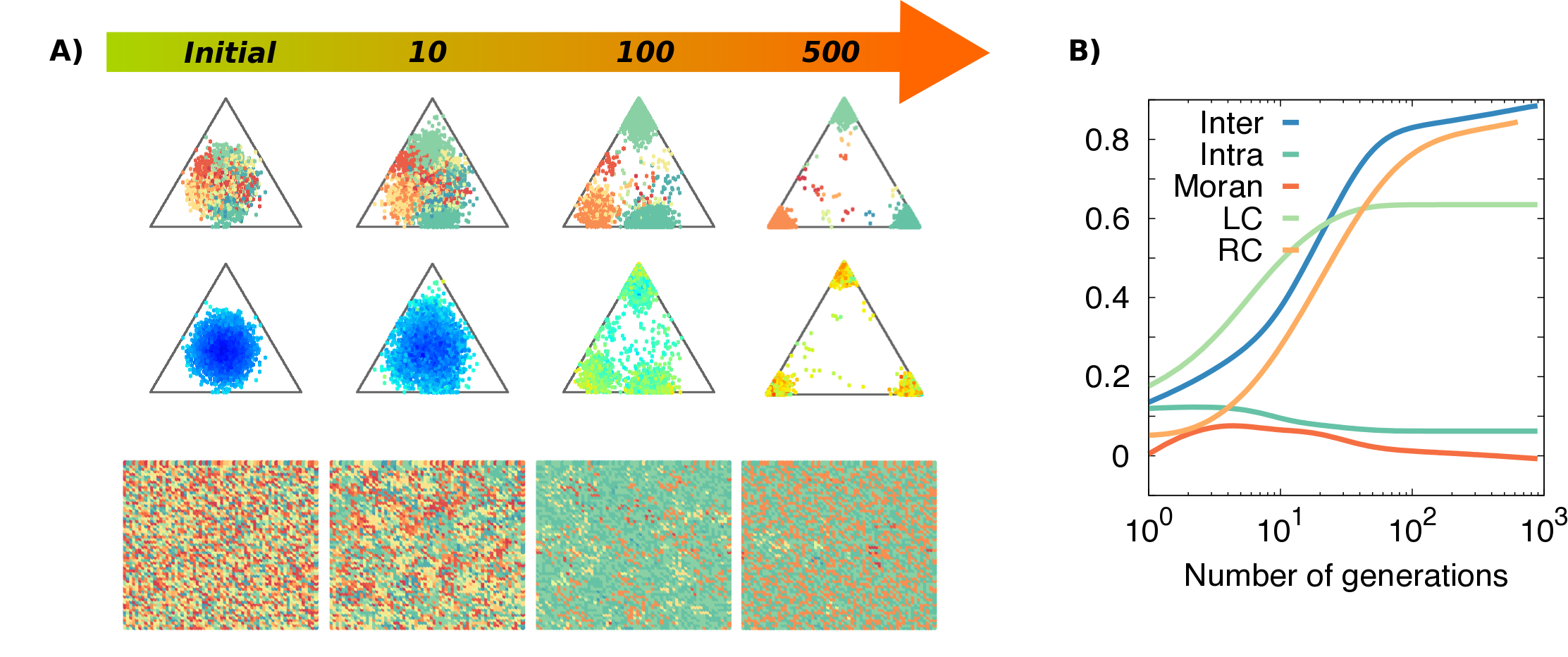
S6. Effect of the competition kernel

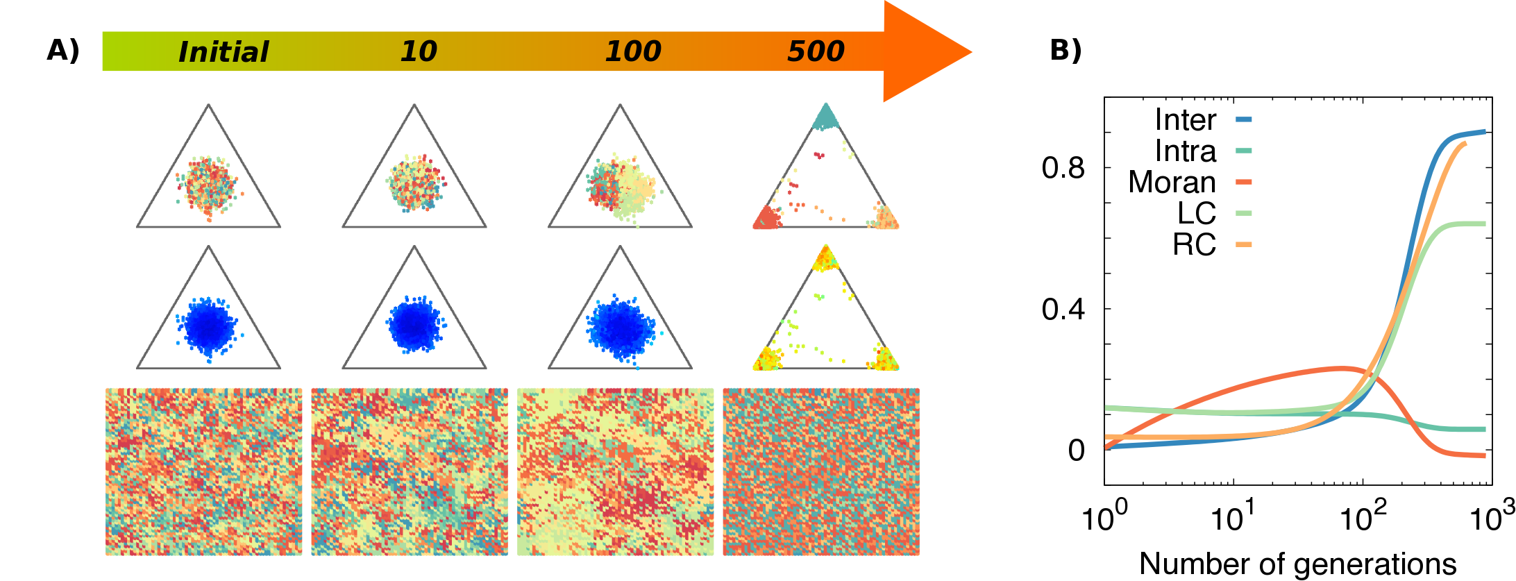
In the implementation of our model presented in the main text, the reproduction probability of an individual $i$ is proportional to $e^{\beta C_{i}}$, where $C_{i}$ is the average trait complementarity among neighbors, $C_{i}=\frac{1}{K}\sum_{j}\frac{1}{n}\sum^{k}|T^{k}(i)-T^{k}(j)|$. However, the use of a non-differentiable argument (absolute value) appearing linearly in the exponential kernel may lead to spurious robust coexistence of arbitrarily similar species (at zero phenotypic distance) (Geritz et al., 1999; Adler and Mosquera, 2000; Hernández-García et al., 2009; Barabás et al., 2013; Lampert and Hastings, 2014). Kernels of the form $e^{\beta C_{i}^{2+\alpha}}$ with $\alpha>0$ have been shown to avoid such artifacts (Pigolotti et al., 2007, 2010). For these reasons, we also considered an alternative competition kernel of the form $e^{\beta C_{i}^{4}}$ to check for the validity and robustness of our conclusions.

Results are shown in Fig 10. We observe that, as the quartic kernel reduces the overall competition of phenotypically similar individuals, it leads to a slower species-diversification process (as compared with the linear one for the same value of the parameters). However, results are qualitatively similar to the linear kernel case. In particular, similar (equivalent) species continue to emerge and coexiste for very long times, as in the linear case. In Appendix SS7. Emergent Neutrality we discuss the coexistence of emergent equivalent species in more detail.

Figure 10: (Color online) Quartic competition kernel. A) From top to bottom: Tradeoff values, trait complementarities, and spatial distributions at different generations. Simulations were run setting the performance of individuals proportional to $e^{\beta C^{4}}$ (rather than $e^{\beta C}$ used in the main text), where $C$ is the average trait complementarity among neighbors. B) Inter and intra-specific distances, local and relative complementarity and Moran’s Index evolution. Parameters: $L=64,S=16,\beta=10,\mu=0.025$.

S7. Emergent Neutrality

In the main text, we discuss the possibility of emerging phenotypically-equivalent species coexisting for long periods of time. It is important to underline that not all realizations lead to equivalent species coexisting in the community. However, this appears to be a significant pattern and we explored it further. In particular, we decided to check the stability of the coexistence. In this Section, we study the mean coexistence time of equivalent species as a measure of coexistence stability.

Two equivalent species coexist until one of them invades the phenotypic space of the other as a result of demographic fluctuations. As a first step to quantify the dynamics of this process, we define a computational criterion to determine equivalence: two species $s_{1}$ and $s_{2}$ are considered equivalent if their inter-specific distance (i.e. distance between their centroids) differs less than a fraction of their mean intraspecific distance (mean trait amplitude), for instance $1/4$, which produces a significant overlap of the clusters of both species in phenotypic space.

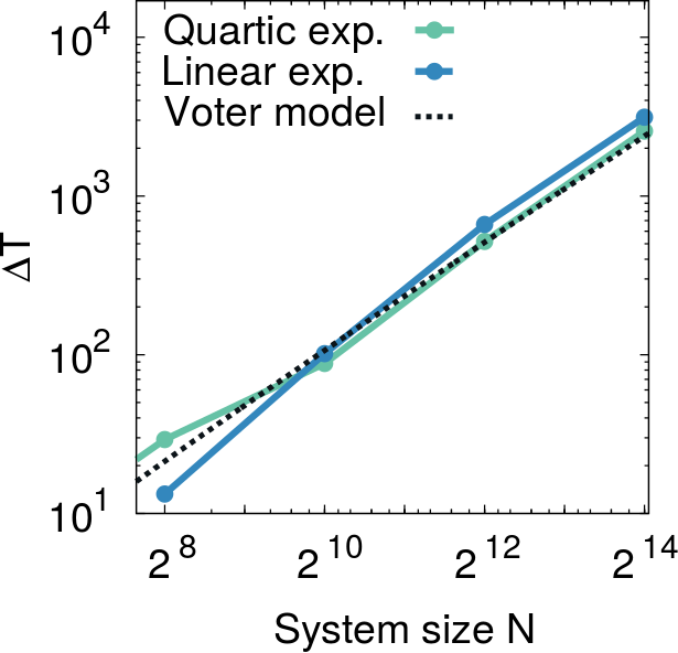
We then measured the mean number of generations $\Delta T$ between the time at which $4$ species remain in the system (with two of them being equivalent, based on the previous definition) and the time at which one of such equivalent species invades the other one. In voter models (i.e. the neutral case), the mean time to reach mono-dominance, $\Delta T$, increases with the number of individuals in the community, $N$; in particular, $\Delta T\sim N\log N$ in a 2D lattice and $\Delta T\sim N$ in a well-mixed situation (for instance, the case of long-distance dispersal and global competition) (Cox, 1989).

Fig. 11 shows $\Delta T$ for simulations with limited dispersal (i.e. the 2D case), as well as the theoretical expectation for the neutral case. To check the robustness of coexistence to the shape of the competition kernel (Geritz et al., 1999; Adler and Mosquera, 2000; Pigolotti et al., 2007; Hernández-García et al., 2009; Pigolotti et al., 2010; Barabás et al., 2013; Lampert and Hastings, 2014) (see Appendix SS6. Effect of the competition kernel), we run simulations using a linear-exponential ($e^{\beta C}$) and a quartic-exponential ($e^{\beta C^{4}}$) kernel, where $C$ is the mean trait complementarity among neighbors. In both cases, our results are compatible with the neutral scenario.

Figure 11: (Color online) Mean number of “ coexistence”, for different system sizes of the community. We show results using a linear-exponential ($e^{\beta C}$) and a quartic-exponential ($e^{\beta C^{4}}$) kernel comparing them with the theoretical expectation for a 2D voter model, $\Delta T\propto N\log N$ (Cox, 1989). Parameters: $L=64,S=8,\beta=10,\mu=0.025$. Deviations from the straight line probably stem from lack of statistics (which is costly at such large sizes/times).

S8. Asymmetrical resource trade-offs

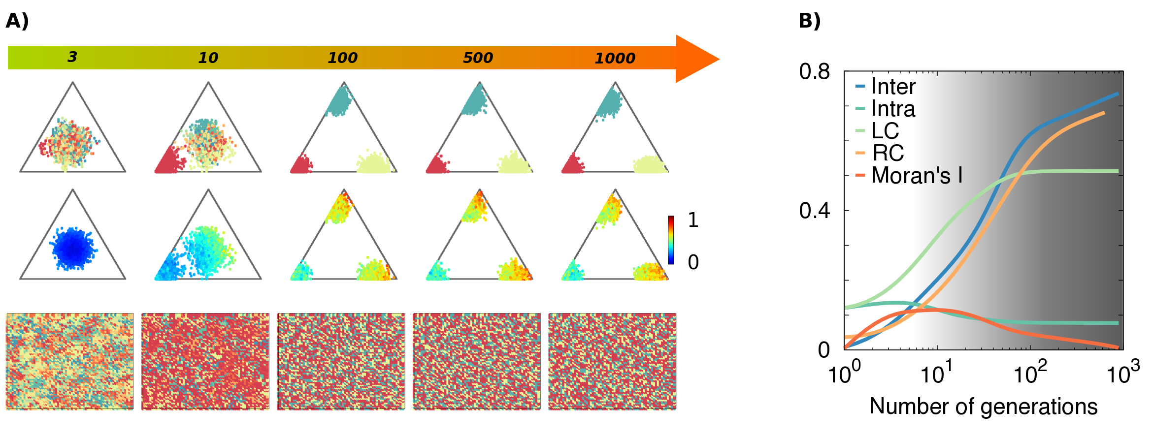
In this section we consider a model variant in which positions in the trade-off space are not equally rewarding a priori. In particular, we chose one of the corners to be favored respect to the others: individuals whose phenotypes are closer to that vertex have a higher probability of reproduction. This could be interpreted as one particular limiting resource being more crucial, or mean that the availability of some resource scales nonlinearly with corresponding trait (e.g., a plant with a short root might not be able to reach a deep water layer. Individuals with longer root systems will have a disproportionate advantage).

In particular, we now modulate the performance of each individual $i$ by multiplying it by a factor $R_{i}=r_{1}T^{1}+r_{2}T^{2}+r_{3}T^{3}$; where $r_{1}$, $r_{2}$ and $r_{3}$ are weights (real numbers in the interval $[0,1]$) such that $r_{1}+r_{2}+r_{3}=1$. For simplicity we fix $r_{1}=(1+2\epsilon)/3$, $r_{2}=r_{3}=(1-\epsilon)/3$ in order to control the asymmetry with a single parameter ($\epsilon$; the symmetric case is $\epsilon=0$), while $\epsilon$ values close to $1$ lead to large asymmetries. In what follows we fix $\epsilon=0.99$.

As illustrated in Fig. 12, although most of individuals initially occupy the most favored (left) corner, after a few generations, some individuals also settle at other available (and less favorable) regions; this is a consequence of the system’s tendency to reduce the level of competition. In conclusion, the main phenomenology reported in the main text appears robust to asymmetrical trade-offs.

Figure 12: (Color online) Asymmetry among trade-offs: A) Trade-off space and complementarity as a function of the number of generations. B) Different measurements characterizing the community in time. Local and relative complementarities confirm that rapid evolutionary changes may within a few generations. Parameters: $L=64$, $S=16$, $\beta=10$, $\mu=0.025$.

S9. Asexual reproduction

Our model adopts the (sexual) reproduction mechanism of the communities considered in the experiments by Zuppinger-Dingley et al. (Zuppinger-Dingley et al., 2014). Here we analyze a case of asexual reproduction in which the traits are directly transmitted from an individual to its offspring (with some variability), i.e. taking $\eta=1$ in our model (see main text).

Fig 13A shows the evolution of individual phenotypes (each trait value $T_{1},T_{2},T_{3}$ is represented by the amount of red, yellow and blue respectively), complementarity and spatial distribution. Observe that, once again, the chief phenomenology of the model, i.e. segregation toward high levels of specialization, is observed. However, in this case, the mechanism of diversification is quite different: individuals from any given species can specialize independently. Thus, in the absence of sexual reproduction, diversification occurs at an individual rather than at a species level. This type of individual differentiation fosters the presence of equivalent species (as the species label becomes completely irrelevant in this setting).

Figure 13: (Color online) Asexual reproduction: A) Tradeoff space and complementarity as a function of the number of generations. Each individual traits values $T_{1},T_{2},T_{3}$ are represented by the amount of red, yellow and blue respectively. Parameter values: $L=64$, $S=16$, $\beta=10$, $\mu=0.025$. Competition avoidance leads individuals to segregate in the trade-off space. B) Local complementarity increases similarly to the main model.

S10. Surviving species

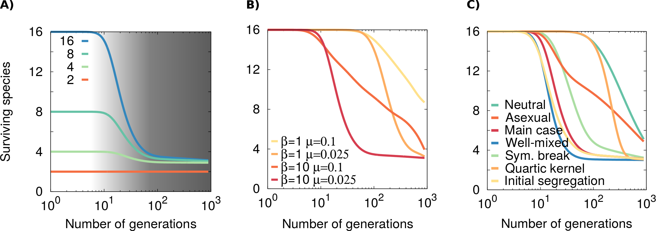
As we do not include mechanisms such as migration or speciation, the number of species actually present in the community can be reduced after several generations. The resulting change in diversity can be regarded as an important attribute, because it illustrates the limit of maximum diversity that a finite system can harbor is the absence of inmigration or speciation processes.

Fig. 14 shows the number of surviving species in different scenarios, including different levels of competition and variability parameters, and other model variants. As expected, extinctions occur more rapidly for higher levels of competition (larger values of $\beta$). The effective level of competition is enhanced in the mean-field case in which all individuals interact with each other (see Appendix SS3. Long-distance dispersal and competition), leading to faster extinction.

In the neutral case ($\beta=0$), species disappear at a very slow rate as there is no competition, but due to stochasticity, most of them are likely to disappear, leading to mono-dominance for sufficiently large timescales (Liggett, 2012). Interestingly, the stable solution in our model with competition ($\beta\neq 0$) consists of multiple species –as many as the niche dimensionality, in this case 3– coexisting for an arbitrarily large number generations. This result is congruent with the “niche dimension hypothesis”, which states that a greater diversity of niches leads to a greater diversity of species (Hutchinson, 1957).

Figure 14: (Color online) Number of surviving species in time for different A) initial number of species, B) competition and variability parameters and C) variants of the model. Species disappear faster in environments with high competition (higher values of $\beta$, or the mean-field). In contrast, the neutral case ($\beta=0$) corresponds to the case in which more species survive after generations, although, due to demographic fluctuations, they still disappear on the long term. For sufficiently large numbers of generations, the system converges to a state with the same number of species than the niche dimensionality ($3$ in our case); these species coexist for arbitrarily long periods (provided the lattice is sufficiently large). Parameter values: $L=64$, and $\beta=10$, and $\mu=0.025$ in A) and C).

References

- Adler and Mosquera [2000] Frederick R Adler and Julio Mosquera. Is space necessary? interference competition and limits to biodiversity. Ecology, 81(11):3226–3232, 2000.
- Allan et al. [2013] Eric Allan, Tania Jenkins, Alexander JF Fergus, Christiane Roscher, Markus Fischer, Jana Petermann, Wolfgang W Weisser, and Bernhard Schmid. Experimental plant communities develop phylogenetically overdispersed abundance distributions during assembly. Ecology, 94(2):465–477, 2013.
- Azaele et al. [2015] Sandro Azaele, Samir Suweis, Jacopo Grilli, Igor Volkov, Jayanth R Banavar, and Amos Maritan. Statistical mechanics of ecological systems: Neutral theory and beyond. arXiv preprint arXiv:1506.01721, 2015.
- Barabás et al. [2012] György Barabás, Simone Pigolotti, Mats Gyllenberg, Ulf Dieckmann, and Géza Meszéna. Continuous coexistence or discrete species? a new review of an old question. Evolutionary Ecology Research, 14(5):523–554, 2012.
- Barabás et al. [2013] György Barabás, Rafael D’Andrea, and Annette Marie Ostling. Species packing in nonsmooth competition models. Theoretical ecology, 6(1):1–19, 2013.
- Bonsall et al. [2004] Michael B Bonsall, Vincent AA Jansen, and Michael P Hassell. Life history trade-offs assemble ecological guilds. Science, 306(5693):111–114, 2004.
- Cardinale et al. [2009] BJ Cardinale, Emmett Duffy, Diane Srivastava, Michel Loreau, Matt Thomas, and Mark Emmerson. Towards a food web perspective on biodiversity and ecosystem functioning. Biodiversity and human impacts, pages 105–120, 2009.
- Carroll et al. [2007] Scott P Carroll, Andrew P Hendry, David N Reznick, and Charles W Fox. Evolution on ecological time-scales. Functional Ecology, 21(3):387–393, 2007.
- Champagnat et al. [2006] Nicolas Champagnat, Régis Ferrière, and Sylvie Méléard. Unifying evolutionary dynamics: From individual stochastic processes to macroscopic models. Theoretical Population Biology, 69(3):297–321, 2006. ISSN 00405809. doi: 10.1016/j.tpb.2005.10.004. URL http://linkinghub.elsevier.com/retrieve/pii/S0040580905001632.
- Chase and Leibold [2003] Jonathan M Chase and Mathew A Leibold. Ecological niches: linking classical and contemporary approaches. University of Chicago Press, 2003.
- Chesson [2000] Peter Chesson. Mechanisms of maintenance of species diversity. Annual review of Ecology and Systematics, pages 343–366, 2000.
- Cordero and Polz [2014] Otto X Cordero and Martin F Polz. Explaining microbial genomic diversity in light of evolutionary ecology. Nature Reviews Microbiology, 12(4):263–273, 2014.
- Cox [1989] J Theodore Cox. Coalescing random walks and voter model consensus times on the torus in zd. The Annals of Probability, pages 1333–1366, 1989.
- Coyne and Orr [2004] Jerry A Coyne and H Allen Orr. Speciation, volume 37. Sinauer Associates Sunderland, MA, 2004.
- Craig MaClean [2005] R. Craig MaClean. Adaptive radiation in microbial microcosms. Journal of Evolutionary Biology, 18(6):1376–1386, 2005. ISSN 1420-9101. doi: 10.1111/j.1420-9101.2005.00931.x. URL http://dx.doi.org/10.1111/j.1420-9101.2005.00931.x.
- Cremer et al. [2011] Jonas Cremer, Anna Melbinger, and Erwin Frey. Evolutionary and population dynamics: A coupled approach. Phys. Rev. E, 84:051921, Nov 2011. doi: 10.1103/PhysRevE.84.051921. URL http://link.aps.org/doi/10.1103/PhysRevE.84.051921.
- De Aguiar et al. [2009] MAM De Aguiar, M Baranger, EM Baptestini, L Kaufman, and Y Bar-Yam. Global patterns of speciation and diversity. Nature, 460(7253):384–387, 2009.
- DeAngelis and Mooij [2005] Donald L DeAngelis and Wolf M Mooij. Individual-based modeling of ecological and evolutionary processes. Annual Review of Ecology, Evolution, and Systematics, pages 147–168, 2005.
- Dieckmann and Doebeli [1999] U Dieckmann and M On Doebeli. On the origin of species by sympatric speciation. Nature, 400(22):354–357, 1999. ISSN 0028-0836. doi: 10.1038/22521. URL http://www.nature.com/nature/journal/v400/n6742/abs/400354a0.html.
- Dieckmann et al. [1995] U Dieckmann, P Marrow, and R Law. Evolutionary cycling in predator-prey interactions: population dynamics and the red queen. Journal of theoretical biology, 176(1):91–102, sep 1995. ISSN 0022-5193. doi: 10.1006/jtbi.1995.0179. URL http://www.sciencedirect.com/science/article/pii/S0022519385701798.
- Dieckmann and Law [1996] Ulf Dieckmann and Richard Law. The dynamical theory of coevolution: a derivation from stochastic ecological processes. Journal of mathematical biology, 34(5-6):579–612, 1996. URL http://link.springer.com/article/10.1007%2FBF02409751.
- Doebeli [2011] Michael Doebeli. Adaptive Diversification (MPB-48). Princeton University Press, 2011.
- Doebeli and Dieckmann [2000] Michael Doebeli and Ulf Dieckmann. Evolutionary branching and sympatric speciation caused by different types of ecological interactions. The american naturalist, 156(S4):S77—-S101, 2000. URL http://www.zoology.ubc.ca/~doebeli/reprints/Doe40.pdf.
- Doebeli and Dieckmann [2003] Michael Doebeli and Ulf Dieckmann. Speciation along environmental gradients. Nature, 421(6920):259–264, 2003. URL http://www.nature.com/nature/journal/v421/n6920/full/nature01274.html.
- Duffy et al. [2007] J Emmett Duffy, Bradley J Cardinale, Kristin E France, Peter B McIntyre, Elisa Thébault, and Michel Loreau. The functional role of biodiversity in ecosystems: incorporating trophic complexity. Ecology letters, 10(6):522–538, 2007.
- Elena and Lenski [2003] Santiago F Elena and Richard E Lenski. Evolution experiments with microorganisms: the dynamics and genetic bases of adaptation. Nature Reviews Genetics, 4(6):457–469, 2003.
- Ellner et al. [2011] Stephen P Ellner, Monica A Geber, and Nelson G Hairston. Does rapid evolution matter? measuring the rate of contemporary evolution and its impacts on ecological dynamics. Ecology Letters, 14(6):603–614, 2011.
- Ford [1975] Edmund Brisco Ford. Ecological genetics. Springer, 1975.
- Friesen et al. [2004] Maren L Friesen, Gerda Saxer, Michael Travisano, and Michael Doebeli. Experimental evidence for sympatric ecological diversification due to frequency-dependent competition in escherichia coli. Evolution, 58(2):245–260, 2004.
- Fussmann et al. [2007a] GF Fussmann, M Loreau, and PA Abrams. Eco-evolutionary dynamics of communities and ecosystems. Functional Ecology, 21(3):465–477, 2007a.
- Fussmann et al. [2007b] GF Fussmann, M Loreau, and PA Abrams. Eco-evolutionary dynamics of communities and ecosystems. Functional Ecology, 21(3):465–477, 2007b.
- Geritz et al. [1998] S.A.H. Geritz, E´. Kisdi, G. Meszéna, and J.A.J. Metz. Evolutionarily singular strategies and the adaptive growth and branching of the evolutionary tree. Evolutionary Ecology, 12(1):35–57, 1998. ISSN 1573-8477. doi: 10.1023/A:1006554906681. URL http://link.springer.com/article/10.1023/A{%}3A1006554906681.
- Geritz et al. [1997] Stefan Geritz, J. Metz, Éva Kisdi, and Géza Meszéna. Dynamics of Adaptation and Evolutionary Branching. Physical Review Letters, 78(10):2024–2027, 1997. ISSN 0031-9007. doi: 10.1103/PhysRevLett.78.2024. URL http://journals.aps.org/prl/abstract/10.1103/PhysRevLett.78.2024.
- Geritz et al. [1999] Stefan AH Geritz, Ed van der Meijden, and Johan AJ Metz. Evolutionary dynamics of seed size and seedling competitive ability. Theoretical population biology, 55(3):324–343, 1999.
- Grace et al. [2016] James B Grace, T Michael Anderson, Eric W Seabloom, Elizabeth T Borer, Peter B Adler, W Stanley Harpole, Yann Hautier, Helmut Hillebrand, Eric M Lind, Meelis Pärtel, et al. Integrative modelling reveals mechanisms linking productivity and plant species richness. Nature, 529(7586):390–393, 2016.
- Grant and Grant [2006] Peter R Grant and B Rosemary Grant. Evolution of character displacement in darwin’s finches. science, 313(5784):224–226, 2006.
- Gravel et al. [2006a] Dominique Gravel, Charles D Canham, Marilou Beaudet, and Christian Messier. Reconciling niche and neutrality: the continuum hypothesis. Ecology letters, 9(4):399–409, 2006a.
- Gravel et al. [2006b] Dominique Gravel, Charles D. Canham, Marilou Beaudet, and Christian Messier. Reconciling niche and neutrality: the continuum hypothesis. Ecology Letters, 9(4):399–409, 2006b.
- Haegeman and Loreau [2011] Bart Haegeman and Michel Loreau. A mathematical synthesis of niche and neutral theories in community ecology. Journal of Theoretical Biology, 269(1):150–165, 2011.
- Hansen et al. [2007] Susse Kirkelund Hansen, Paul B Rainey, Janus AJ Haagensen, and Søren Molin. Evolution of species interactions in a biofilm community. Nature, 445(7127):533–536, 2007.
- Hanski [2012] Ilkka Hanski. Eco-evolutionary dynamics in a changing world. Annals of the New York Academy of Sciences, 1249(1):1–17, 2012. ISSN 00778923. doi: 10.1111/j.1749-6632.2011.06419.x. URL http://doi.wiley.com/10.1111/j.1749-6632.2011.06419.x.
- Harpole and Tilman [2007] W Stanley Harpole and David Tilman. Grassland species loss resulting from reduced niche dimension. Nature, 446(7137):791–793, 2007.
- Hernández-García et al. [2009] Emilio Hernández-García, Cristóbal López, Simone Pigolotti, and Ken H Andersen. Species competition: coexistence, exclusion and clustering. Philosophical Transactions of the Royal Society of London A: Mathematical, Physical and Engineering Sciences, 367(1901):3183–3195, 2009.
- Herron and Doebeli [2013] Matthew D Herron and Michael Doebeli. Parallel evolutionary dynamics of adaptive diversification in escherichia coli. PLoS Biol, 11(2):e1001490, 2013.
- Hooper et al. [2005] David U Hooper, FS Chapin Iii, JJ Ewel, Andy Hector, Pablo Inchausti, Sandra Lavorel, JH Lawton, DM Lodge, Michel Loreau, S Naeem, et al. Effects of biodiversity on ecosystem functioning: a consensus of current knowledge. Ecological monographs, 75(1):3–35, 2005.
- Hubbell [2001] Stephen P Hubbell. The unified neutral theory of biodiversity and biogeography (MPB-32), volume 32. Princeton University Press, 2001.
- Hutchinson [1957] G.E. Hutchinson. Concluding remarks. Cold Spring Harbor Symposia on Quantitative Biology, 22(2):415–427, 1957.
- Jansen and Mulder [1999] VAA Jansen and GSEE Mulder. Evolving biodiversity. Ecology Letters, 2(6):379–386, 1999.
- Johnson and Stinchcombe [2007] Marc TJ Johnson and John R Stinchcombe. An emerging synthesis between community ecology and evolutionary biology. Trends in Ecology & Evolution, 22(5):250–257, 2007.
- Lampert and Hastings [2014] Adam Lampert and Alan Hastings. Sharp changes in resource availability may induce spatial nearly periodic population abundances. Ecological Complexity, 19:80–83, 2014.
- Law et al. [1997] Richard Law, Paul Marrow, and U Dieckmann. On evolution under asymmetric competition. Evolutionary Ecology, 11(4):485–501, 1997. doi: http://dx.doi.org/10.1023/A:1018441108982. URL http://link.springer.com/article/10.1023/A:1018441108982.
- Levin [1992] SA Levin. The problem of scale and pattern in ecology. Ecology, 73(1943):1967, 1992.
- Liggett [2012] Thomas Liggett. Interacting particle systems, volume 276. Springer Science & Business Media, 2012.
- Loeuille and Loreau [2004] Nicolas Loeuille and Michel Loreau. Nutrient enrichment and food chains: can evolution buffer top-down control? Theoretical population biology, 65(3):285–298, 2004.
- Loreau and Hector [2001] Michel Loreau and Andy Hector. Partitioning selection and complementarity in biodiversity experiments. Nature, 412(6842):72–76, 2001.
- MacArthur and Levins [1967] Robert MacArthur and Richard Levins. The limiting similarity, convergence, and divergence of coexisting species. American Naturalist, pages 377–385, 1967.
- MacArthur [1984] Robert H MacArthur. Geographical ecology: patterns in the distribution of species. Princeton University Press, 1984.
- May and Mac Arthur [1972] Robert M May and Robert H Mac Arthur. Niche overlap as a function of environmental variability. Proceedings of the National Academy of Sciences, 69(5):1109–1113, 1972.
- Miettinen [1999] Kaisa Miettinen. Nonlinear multiobjective optimization, volume 12. Springer Science & Business Media, 1999.
- Moran [1950] Patrick AP Moran. Notes on continuous stochastic phenomena. Biometrika, pages 17–23, 1950.
- Pianka [1974] Eric R Pianka. Niche overlap and diffuse competition. Proceedings of the National Academy of Sciences, 71(5):2141–2145, 1974.
- Pigolotti et al. [2007] Simone Pigolotti, Cristóbal López, and Emilio Hernández-García. Species clustering in competitive lotka-volterra models. Physical review letters, 98(25):258101, 2007.
- Pigolotti et al. [2010] Simone Pigolotti, Cristóbal López, Emilio Hernández-García, and Ken H Andersen. How gaussian competition leads to lumpy or uniform species distributions. Theoretical Ecology, 3(2):89–96, 2010.
- Rainey and Travisano [1998] Paul B Rainey and Michael Travisano. Adaptive radiation in a heterogeneous environment. Nature, 394(6688):69–72, 1998.
- Ramos et al. [2008] Francisco Ramos, Cristóbal López, Emilio Hernández-García, and Miguel A Muñoz. Crystallization and melting of bacteria colonies and brownian bugs. Physical Review E, 77(2):021102, 2008.
- Reiss et al. [2009] Julia Reiss, Jon R Bridle, Jose M Montoya, and Guy Woodward. Emerging horizons in biodiversity and ecosystem functioning research. Trends in ecology & evolution, 24(9):505–514, 2009.
- Rosenzweig [1995] Michael L Rosenzweig. Species diversity in space and time. Cambridge University Press, 1995.
- Rosindell et al. [2011] James Rosindell, Stephen P Hubbell, and Rampal S Etienne. The unified neutral theory of biodiversity and biogeography at age ten. Trends in ecology & evolution, 26(7):340–348, 2011.
- Rulands et al. [2014] Steffen Rulands, David Jahn, and Erwin Frey. Specialization and bet hedging in heterogeneous populations. Physical review letters, 113(10):108102, 2014.
- Scheffer and van Nes [2006a] Marten Scheffer and Egbert H van Nes. Self-organized similarity, the evolutionary emergence of groups of similar species. Proceedings of the National Academy of Sciences, 103(16):6230–6235, 2006a.
- Scheffer and van Nes [2006b] Marten Scheffer and Egbert H. van Nes. Self-organized similarity, the evolutionary emergence of groups of similar species. Proc Natl Acad of Sci USA, 103(16):6230–6235, 2006b. doi: 10.1073/pnas.0508024103.
- Schluter [2000] Dolph Schluter. The ecology of adaptive radiation. Oxford University Press, 2000.
- Schoener [2011] Thomas W Schoener. The newest synthesis: understanding the interplay of evolutionary and ecological dynamics. science, 331(6016):426–429, 2011.
- Slatkin [1980] Montogemery Slatkin. Ecological character displacement. Ecology, 61(1):163–177, 1980.
- Spencer et al. [2007] Christine C Spencer, Melanie Bertrand, Michael Travisano, and Michael Doebeli. Adaptive diversification in genes that regulate resource use in escherichia coli. PLoS Genet, 3(1):e15, 2007.
- Strauss et al. [2008] Sharon Y Strauss, Jennifer A Lau, Thomas W Schoener, and Peter Tiffin. Evolution in ecological field experiments: implications for effect size. Ecology Letters, 11(3):199–207, 2008.
- Stuart et al. [2014] Y. E. Stuart, T. S. Campbell, P. A. Hohenlohe, R. G. Reynolds, L. J. Revell, and J. B. Losos. Rapid evolution of a native species following invasion by a congener. Science, 346(6208):463–466, 2014.
- Taper and Case [1992] Mark L Taper and Ted J Case. Models of character displacement and the theoretical robustness of taxon cycles. Evolution, pages 317–333, 1992.
- Thompson [1998] John N Thompson. Rapid evolution as an ecological process. Trends in Ecology & Evolution, 13(8):329–332, 1998.
- Tilman [1988] David Tilman. Plant strategies and the dynamics and structure of plant communities. Number 26. Princeton University Press, 1988.
- Tilman [2004] David Tilman. Niche tradeoffs, neutrality, and community structure: a stochastic theory of resource competition, invasion, and community assembly. Proceedings of the National Academy of Sciences of the United States of America, 101(30):10854–10861, 2004.
- Tilman and Snell-Rood [2014] David Tilman and Emilie C Snell-Rood. Ecology: Diversity breeds complementarity. Nature, 515:44–45, 2014.
- Tilman et al. [2006] David Tilman, Peter B Reich, and Johannes MH Knops. Biodiversity and ecosystem stability in a decade-long grassland experiment. Nature, 441(7093):629–632, 2006.
- Tyerman et al. [2005] Jabus Tyerman, Naomi Havard, Gerda Saxer, Michael Travisano, and Michael Doebeli. Unparallel diversification in bacterial microcosms. Proceedings of the Royal Society of London B: Biological Sciences, 272(1570):1393–1398, 2005.
- Volkov et al. [2003] I. Volkov, J.I. Banavar, S.P. Hubbell, and A. Maritan. Neutral theory and relative species abundance in ecology. Nature, 424:1035–1037, 2003.
- Yoshida et al. [2003] Takehito Yoshida, Laura E Jones, Stephen P Ellner, Gregor F Fussmann, and Nelson G Hairston. Rapid evolution drives ecological dynamics in a predator–prey system. Nature, 424(6946):303–306, 2003.
- Zuppinger-Dingley et al. [2014] Debra Zuppinger-Dingley, Bernhard Schmid, Jana S Petermann, Varuna Yadav, Gerlinde B De Deyn, and Dan FB Flynn. Selection for niche differentiation in plant communities increases biodiversity effects. Nature, 515(7525):108–111, 2014.