The environmental dependence of the baryon acoustic peak in the Baryon Oscillation Spectroscopic Survey CMASS sample

Abstract

The environmental dependence of galaxy clustering encodes information about the physical processes governing the growth of cosmic structure. We analyze the baryon acoustic peak as a function of environment in the galaxy correlation function of the Baryon Oscillation Spectroscopic Survey CMASS sample. Dividing the sample into three subsets by smoothed local overdensity, we detect acoustic peaks in the six separate auto-correlation and cross-correlation functions of the sub-samples. Fitting models to these correlation functions, calibrated by mock galaxy and dark matter catalogues, we find that the inferred distance scale is independent of environment, and consistent with the result of analyzing the combined sample. The shape of the baryon acoustic feature, and the accuracy of density-field reconstruction in the Zeldovich approximation, varies with environment. By up-weighting underdense regions and down-weighting overdense regions in their contribution to the full-sample correlation function, by up to $50\%$, we achieve a fractional improvement of a few per cent in the precision of baryon acoustic oscillation fits to the CMASS data and mock catalogues: the scatter in the preferred-scale fits to the ensemble of mocks improves from $1.45\%$ to $1.34\%$ (pre-reconstruction) and $1.03\%$ to $1.00\%$ (post-reconstruction). These results are consistent with the notion that the acoustic peak is sharper in underdense environments.

1 Introduction

Baryon acoustic oscillations (BAO) are a feature of the 2-point clustering pattern of galaxies which encodes a preferred co-moving separation of order $100\,h^{-1}$Mpc – the sound horizon at the baryon drag epoch. The feature manifests as a small but discernible peak in the galaxy correlation function, and as a series of harmonics in the galaxy power spectrum.

BAO in large-scale structure have emerged as an important cosmological probe because this preferred length scale, calibrated by early-Universe physics established by the Cosmic Microwave Background, may be used as a standard ruler to map out the cosmic distance scale and expansion rate as a function of redshift (Eisenstein et al., 1998; Blake & Glazebrook, 2003; Seo & Eisenstein, 2003; Eisenstein et al., 2005). Recent large-scale structure surveys have used BAO to report distance-scale measurements for redshifts $z<2.3$ with accuracies in the range $1-5\%$ (Blake et al., 2011; Beutler et al., 2011; Padmanabhan et al., 2012; Kazin et al., 2014; Anderson et al., 2014; Ross et al., 2015; Bautista et al., 2017; Alam et al., 2017; Ata et al., 2018). These measurements are consistent with the distance-redshift relation inferred from analysis of the Cosmic Microwave Background, in the context of the $\Lambda$CDM model and FLRW metric (Planck Collaboration et al., 2018).

Although the baryon acoustic peak is a robust prediction of early-Universe physics (Eisenstein & White, 2004), its presence in the late-time clustering pattern is modulated by non-linear effects such as the growth of structure, redshift-space distortions and galaxy bias (Eisenstein et al., 2007a; Smith et al., 2008; Seo et al., 2008; Crocce & Scoccimarro, 2008; Matsubara, 2008). These modifications may be used either as a source of additional cosmological information, or as a mechanism for enhancing the accuracy of the standard ruler by approximately recovering the pristine information from early times.

An important property of the late-time acoustic peak is a broadening caused by the displacement of galaxies from their original locations in the density field, produced by bulk-flow motions which trace the contraction of overdense regions and expansion of voids (Eisenstein et al., 2007a; Sherwin & Zaldarriaga, 2012; McCullagh et al., 2013; Rasera et al., 2014). These displacements may be estimated in linear perturbation theory from the density field traced by the galaxies, and partially retracted in order to sharpen the peak profile, in a process known as density-field reconstruction (Eisenstein et al., 2007b; Padmanabhan et al., 2009). The statistical properties of the galaxy displacements and the accuracy of the reconstruction algorithm depend on local environment, which controls the growth of structure and applicability of linear theory (Achitouv & Blake, 2015).

As a consequence of these effects, the profile of the baryon acoustic peak depends on local environment (Neyrinck et al., 2018). In this paper we will map out this environmental dependence using the largest current galaxy large-scale structure dataset, the Baryon Oscillation Spectroscopic Survey (BOSS) (Dawson et al., 2013; Reid et al., 2016; Alam et al., 2017). Our motivation is two-fold. First, if the acoustic peak shape depends on environment, then using a fitting template matched to each environment might result in an improved error in the distance-scale fit. Second, if the sharpness of the baryon acoustic peak is a function of environment, or if density-field reconstruction is less accurate in dense environments owing to the increased importance of non-linear effects, then enhancing the weight of low-density environments might also improve the fit (Achitouv & Blake, 2015).

A number of previous studies have explored the behaviour of the baryon acoustic peak in the context of environment, with different emphasis and aims. Neyrinck et al. (2018) found that the location of the acoustic peak in the correlation function of N-body dark matter simulations was shifted as a function of environment by a few per cent, due to the contraction of overdense regions and expansion of underdense regions. This effect was investigated using the Luminous Red Galaxy dataset of the Sloan Digital Sky Survey by Roukema et al. (2015), who reported that the acoustic peak is compressed by a similar factor for galaxy pairs spanning supercluster regions. Kitaura et al. (2016) detected the acoustic peak in the correlation function of a sample of voids constructed from the BOSS dataset, and Zhao et al. (2018) explored the additional distance-scale information that resulted when these void measurements were combined with galaxy clustering. Although we focus on correlation function analysis in this paper, we note that clustering statistics sensitive to environment may be constructed in several different ways, such as the sliced correlation function (Neyrinck et al., 2018), the density-marked correlation function (White, 2016) and as position-dependent clustering sensitive to higher-order correlations (Chiang et al., 2014). Finally, density-dependent effects may be linked to a rich set of theoretical phenomenology, such as screening mechanisms in modified gravity scenarios (Falck et al., 2015) or the imprint of an inhomogeneous cosmological metric (Roukema et al., 2016).

This paper is structured as follows. In Section 2 we present the data and mock catalogues utilized in our analysis, our definitions of local environment, and our procedures for estimating the galaxy correlation function within environmental slices and weighting pair counts as a function of overdensity. In Section 3 we describe our approach for fitting BAO models as a function of environment, and in Section 4 we summarize the results of our distance-scale fits to the environmental and weighted correlation functions. We present our conclusions in Section 5.

2 Measurements

2.1 Data and mock catalogues

Our study is based on the final data release (DR12) of the Baryon Oscillation Spectroscopic Survey (Dawson et al., 2013; Reid et al., 2016; Alam et al., 2017). In particular we analyzed the largest component of BOSS, the CMASS Luminous Red Galaxy sample, which was selected by optical colour and magnitude cuts to form an approximately stellar-mass limited sample of almost 1 million massive galaxies in the redshift range $0.43<z<0.7$. The sample is divided into two contiguous regions of sky, covering the Northern Galactic Cap (NGC) and Southern Galactic Cap (SGC), which together span an effective volume of $5.1$ Gpc³ for cosmological purposes (Reid et al., 2016), with an effective redshift $z_{\rm eff}=0.57$ which we adopted in this analysis.

CMASS galaxies are assigned a combination of weights for clustering analysis (Reid et al., 2016): observational systematics weights, which correct for non-cosmological density fluctuations induced by varying stellar density and seeing, weights which compensate for missing objects due to fibre collisions or redshift failures, and FKP weights (Feldman et al., 1994) which optimally balance the contribution of sample variance and Poisson noise to clustering measurements. We applied all of these weights in our correlation function analysis. We also utilized the accompanying CMASS random catalogues, which are around 50 times larger than the galaxy dataset, and constructed to match its redshift distribution and angular coverage.

Mock galaxy catalogues are an integral part of clustering studies, allowing us to test model-fitting procedures on a simulated dataset with known input cosmology, and determine covariance matrices from the ensemble of mocks. Our analysis utilized 600 Quick Particle Mesh (QPM) mock galaxy catalogues (White et al., 2014) accompanying the CMASS dataset. These mock catalogues are built from low-resolution particle-mesh simulations, from which sub-samples of particles are drawn with properties approximately matching the distribution and clustering statistics of dark matter halos. These halo tracers are populated with a halo occupation distribution and sub-sampled to match the selection function and clustering of the CMASS sample (see Alam et al. (2017) for a summary of the mock catalogues generated for BOSS clustering analyses).

As discussed in Section 1, galaxies are displaced from their original positions in the density field by bulk motions induced by the growth of cosmic structure (Eisenstein et al., 2007b); these motions broaden and dilute the baryon acoustic feature. We computed the displacement field in the Zeldovich approximation of the data and mock catalogues, and corresponding random samples, using the Fourier-space algorithm introduced by Burden et al. (2015). We used this displacement field to retract objects to their near-original positions and hence sharpen the acoustic peak. In the following sections we will present results before and after this density-field reconstruction procedure.

We constructed one of our models for the dependence of the baryon acoustic peak shape on environment using matched N-body dark matter simulations evolved from two sets of initial conditions: a standard fiducial power spectrum containing baryon acoustic oscillations, and a “no-wiggles” power spectrum which closely follows the smooth power spectrum shape of the first simulation, removing the oscillations (Eisenstein & Hu, 1998). Through comparison of the resulting clustering patterns as a function of environment, the effects on the baryon acoustic peak may be distinguished from other clustering properties, and the difference used to construct models. These simulation datasets were specifically generated to investigate BAO in Rasera et al. (2014). They cover a volume of $388$ Gpc³ using $8.6$ billion particles and are part of the Dark Energy Universe Simulation (DEUS) suite (Alimi et al., 2012; Rasera et al., 2014).

Different fiducial cosmological models, summarized in Table 1, were used to map the angular positions and redshifts of CMASS galaxies into co-moving co-ordinates, and to construct the mock catalogues discussed above. Given that the theoretical sound horizon scale depends on the fiducial matter and baryon densities, and its observed position in the correlation function is distorted by Alcock-Paczynski effects in a trial cosmology, these differences are important to track. We analyzed the clustering of the CMASS sample and accompanying QPM mock catalogues, and performed density-field reconstruction, using the BOSS DR12 fiducial cosmology (Alam et al., 2017) listed in the second column of Table 1. However, the QPM mock catalogues and DEUS simulations were constructed from fiducial power spectra of different cosmological models, with varying sound-horizon scales, as summarized in the third and fourth columns of Table 1. These differences were fully accounted in our BAO-fitting process, as explained in Section 3.

Table 1: The fiducial cosmological models relevant to our analysis. We measured correlation functions from the CMASS data and QPM mocks using the “BOSS DR12” fiducial cosmology listed in the second column. This model differs from the cosmology used to construct the initial power spectrum of the QPM mocks (third column) and the DEUS wiggles and no-wiggles dark matter simulations (fourth column). The sound horizon at baryon drag, $r_{s}(z_{d})$, is computed for each cosmological model from CAMB; our value of $r_{s}(z_{d})$ for the BOSS DR12 fiducial cosmology differs slightly from that quoted in Alam et al. (2017) because we assume $\Omega_{\nu}=0$. The final row of the table lists the volume-weighted distance $D_{V}$ for each cosmological model, evaluated at the effective redshift $z=0.57$.

Parameter	BOSS DR12	QPM mock	DEUS
$\Omega_{\rm m}$	$0.31$	$0.29$	$0.2573$
$\Omega_{\rm b}$	$0.0481$	$0.0459$	$0.0436$
$h$	$0.676$	$0.7$	$0.72$
$\sigma_{8}$	$0.8$	$0.8$	$0.801$
$n_{s}$	$0.97$	$0.97$	$0.963$
$r_{s}(z_{d})$ [Mpc]	$147.62$	$147.1$	$149.37$
$D_{V}(z=0.57)$ [Mpc]	$2059.6$	$2009.5$	$1988.2$

2.2 Defining and weighting the environments

In this study we investigate the dependence of the large-scale correlation function of the CMASS galaxy dataset on local environment. We defined environment as the local overdensity of the galaxy sample, $\delta(\vec{x})$ at position $\vec{x}$, smoothed using a Gaussian filter with standard deviation $15\,h^{-1}$Mpc,

$$\delta(\vec{x})=\frac{N_{R}}{N_{D}}\,\frac{\rm{Sm}(D)}{\rm{Sm}(R)}-1,$$ (1)

where ${\rm Sm}()$ represents the application of Gaussian smoothing to the data catalogue ($D$) containing $N_{D}$ galaxies, or the random catalogue ($R$) of $N_{R}$ points.

The adopted smoothing scale of $15\,h^{-1}$Mpc and resulting overdensity field are identical to those used in the density-field reconstruction of the sample (Burden et al., 2015; Alam et al., 2017). The dependence of the performance of reconstruction on smoothing scale has been investigated by Vargas-Magaña et al. (2017) and Achitouv & Blake (2015). For the CMASS sample, the recovered isotropic baryon acoustic scale is insensitive to the choice of smoothing scale within the range $5$ to $15\,h^{-1}$Mpc, although smoothing scales closer to $5\,h^{-1}$Mpc may yield better performance for anisotropic fits (Vargas-Magaña et al., 2017) or for a dataset with higher number density (Achitouv & Blake, 2015).

Following the construction of the smoothed density field, we assigned values of $\delta$ to the data and random points using cloud-in-cell interpolation. The frequency distribution of $\delta$ across the survey volume (i.e. of the random points) is displayed as the blue solid curve in Figure 1, together with the distribution of overdensities assigned to the galaxies as the red dashed curve, which is naturally skewed towards higher values of $\delta$, given that more galaxies are located in overdense environments.

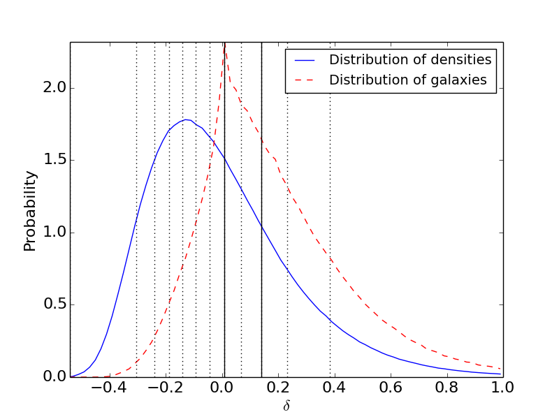
Figure 1: The distribution of overdensity values $\delta$ within the CMASS-North region grid as traced by random points (solid blue histogram), and as traced by CMASS-North galaxies (dashed red histogram, whose distribution is naturally skewed towards higher values of $\delta$). The vertical dotted lines separate the 12 narrow density bins in which we initially measured the galaxy pair counts, and the vertical solid lines separate the 3 environmental slices we used to construct the final galaxy auto-correlation and cross-correlation functions.

We defined $N_{\rm env}=12$ narrow density bins by dividing the survey such that each bin contains equal volume; these bin divisions are displayed as the vertical dotted lines in Figure 1. We ultimately grouped these environments into clustering measurements in 3 density slices, such that the baryon acoustic peak could be detected in each correlation function. Initially measuring the pair counts in narrow bins afforded us the flexibility to adjust the groupings within the coarser bins, without needing to repeat the original pair count measurements.

In addition to constraining any variation of the acoustic peak scale with environment, we also wished to investigate whether acoustic peak measurements may be improved by weighting pair counts as a function of environment. Following Achitouv & Blake (2015), we adopted a simple weighting scheme where the weights $w_{i}$ of the $N_{\rm env}=12$ environments ($1\leq i\leq N_{\rm env}$) varied uniformly as,

$$w_{i}=1+x\left[\frac{2\,(i-1)}{N_{\rm env}-1}-1\right],$$ (2)

in terms of a single parameter $x$ constrained to lie in the range $-1\leq x\leq 1$. Hence, for a given choice of $x$, $w_{i}$ varied uniformly from $1-x$ to $1+x$, such that negative values of $x$ have the effect of upweighting underdense environments with respect to overdense environments.

2.3 Estimating the environmental correlation function

The difference in the distribution of environments in which data and random points reside (Figure 1) complicates the estimation of the correlation function within an environment slice: if the redshift distributions of the parent data and random samples are consistent when averaged over all environments, then the redshift distributions of the corresponding environmental sub-samples will disagree. Therefore, the parent random catalogue requires a redshift-dependent sub-sampling or weighting in order to match the galaxy redshift distribution in a density slice, and provide appropriate pair counts for estimating the environmental correlation function.

We implemented this procedure by measuring pair counts in bins of environment, separation and redshift (co-moving distance in the fiducial cosmology), and then scaling the resulting counts as a function of redshift in the manner described below. We used the 12 environment bins defined in Section 2.2, 36 separation bins of width $5\,h^{-1}$ Mpc between $0$ and $180\,h^{-1}$ Mpc, and 14 bins of co-moving distance of width $50\,h^{-1}$ Mpc between $1100$ and $1800\,h^{-1}$ Mpc. We hence measured the data-data pair counts $dd_{ijkl}(s)$, data-random pair counts $dr_{ijkl}(s)$ and random-random pair counts $rr_{ijkl}(s)$ in separation bins $s$, between bins of environment (denoted by indices $i$ and $j$ for the two catalogues entering the pair count) and redshift (denoted by indices $k$ and $l$ for the two catalogues). We measured pair counts using the corrfunc software (Sinha, 2016).

We now outline how we weighted these pair counts when measuring the galaxy correlation function in a density slice $I$, consisting of some combination of the environments $i$, and the cross-correlation function of galaxies in density slices $I$ and $J$. We also allowed for weighting the contribution of each environment $i$ to the pair count by $w_{i}$, as defined in Equation 2. In the following, we write the number of data and random points in environment $i$ and redshift bin $k$ as $n_{D,ik}$ and $n_{R,ik}$, respectively.

The weighted number of data and random sources in each redshift bin $k$, summed over the combination of environments $i$ for which we wish to measure the correlation function, is then,

$$\begin{split}N_{D,Ik}&=\sum_{i}w_{i}\,n_{D,ik},\\ N_{R,Ik}&=\sum_{i}w_{i}\,n_{R,ik},\end{split}$$ (3)

with total numbers of objects in the density slice,

$$\begin{split}N_{D,I}&=\sum_{i}\sum_{k}w_{i}\,n_{D,ik},\\ N_{R,I}&=\sum_{i}\sum_{k}w_{i}\,n_{R,ik}.\end{split}$$ (4)

We defined weighted pair counts between density slices $I$ and $J$, summed over the corresponding environmental sub-samples $i$ and $j$ and redshift bins $k$ and $l$, as,

$$\begin{split}DD_{IJ}(s)&=\sum_{i}\sum_{j}\sum_{k}\sum_{l}w_{i}\,w_{j}\,dd_{ijkl}(s),\\ DR_{IJ}(s)&=\sum_{i}\sum_{j}\sum_{k}\sum_{l}w_{i}\,w_{j}\,\frac{N_{D,l}}{N_{R,l}}\,dr_{ijkl}(s),\\ RD_{IJ}(s)&=\sum_{i}\sum_{j}\sum_{k}\sum_{l}w_{i}\,w_{j}\,\frac{N_{D,k}}{N_{R,k}}\,dr_{jilk}(s),\\ RR_{IJ}(s)&=\sum_{i}\sum_{j}\sum_{k}\sum_{l}w_{i}\,w_{j}\,\frac{N_{D,k}}{N_{R,k}}\,\frac{N_{D,l}}{N_{R,l}}\,rr_{ijkl}(s).\end{split}$$ (5)

Finally, we estimated the correlation function between density slices $I$ and $J$ using the estimator (Landy & Szalay, 1993),

$$\xi_{IJ}(s)=\frac{DD_{IJ}(s)-DR_{IJ}(s)-RD_{IJ}(s)+RR_{IJ}(s)}{RR_{IJ}(s)}.$$ (6)

When estimating the post-reconstruction correlation function, we also measured the pair counts of the random catalogue shifted by the displacement field, denoted by $S$, such that (Padmanabhan et al., 2012),

$$\xi_{IJ}(s)=\frac{DD_{IJ}(s)-DS_{IJ}(s)-SD_{IJ}(s)+SS_{IJ}(s)}{RR_{IJ}(s)}.$$ (7)

2.4 Correlation function measurements

We used the approach described in Section 2.3 to measure the environmental auto- and cross-correlation functions $\xi_{IJ}$ of the BOSS DR12 CMASS sample, the QPM mock catalogues, and the DEUS wiggles and no-wiggles dark matter simulations. We performed these measurements in three density slices $I,J=\{1,2,3\}$ where, if the survey volume elements are ranked in order of increasing local overdensity, the three slices span volumes in the ratio 7:2:3 (and are constructed by summing pair counts for corresponding numbers of the original 12 narrow environment bins). The three density slices correspond to overdensity ranges $-1<\delta<0.01$, $0.01<\delta<0.14$ and $\delta>0.14$ for $I,J=\{1,2,3\}$, respectively. We chose these three density slices ensuring that we detected the baryon acoustic peak in each individual auto- and cross-correlation function. Given that $\xi_{JI}=\xi_{IJ}$, our three density slices yielded six correlation functions, $\{\xi_{11},\xi_{12},\xi_{13},\xi_{22},\xi_{23},\xi_{33}\}$. We also measured the total correlation functions $\xi_{\rm tot}$ combining all environments of the different samples, and the weighted correlation functions for different values of the parameter $x$ defined in Equation 2, spaced by $\Delta x=0.2$ in the range $-1<x<1$.

By determining the same correlation functions for the ensemble of mock catalogues, we built a covariance matrix spanning the $\xi_{IJ}$ measurements for different density slices and scales. For the BOSS DR12 data and mock catalogues, we measured separate correlation functions for the NGC and SGC survey regions, and combined these measurements using inverse-variance weighting based on the correlation function errors determined from the mocks.

Figure 2 displays the mean of the total and environmental correlation functions of the QPM mock catalogues, before and after density-field construction, as the dashed and solid lines, respectively. We present these measurements after subtracting the smooth “no-wiggles” component of the correlation function model, described in more detail in Section 3, to facilitate comparison of the acoustic peak shape. We find that the peak shape depends on density, with the environmental correlation functions exhibiting more prominent negative “wings” on either side of the peak than the total correlation function, and the amplitude of the baryon acoustic feature increasing steadily towards underdense environments, varying by a factor of around two. Density-field reconstruction sharpens the acoustic peaks as expected. We consider the distance-scale fits to the correlation functions in Section 4 below.

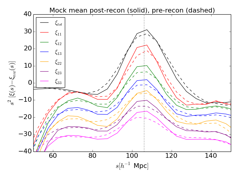
Figure 2: The mean auto-correlation and cross-correlation functions $\xi_{IJ}(s)$ of the CMASS QPM mock galaxy catalogues in three environmental slices defined by increasing local density, compared to the total correlation function $\xi_{\rm tot}$. In order to highlight the behaviour of the baryon acoustic peak, we subtracted a “no-wiggles” correlation function model from each measurement and scaled the resulting difference by $s^{2}$. The solid and dashed lines display the correlation functions after and before reconstruction, respectively. Successive correlation functions have been offset in the $y$-direction by $\Delta y=-5$, for clarity of presentation. The acoustic peak shape varies with environment. The vertical dotted line, plotted at the approximate correlation function peak, indicates that the preferred scale does not vary significantly with environment.

Figure 3 presents the measurements of the auto- and cross-correlation functions $\xi_{IJ}$ in density slices for the DR12 CMASS data sample, before reconstruction (upper panel) and after reconstruction (lower panel). The errors in the measurements are determined from the diagonal elements of the covariance matrix built from the mock catalogues. We detect the baryon acoustic feature in all six of the post-reconstruction correlation functions, and we describe the fitted BAO models in the following section.

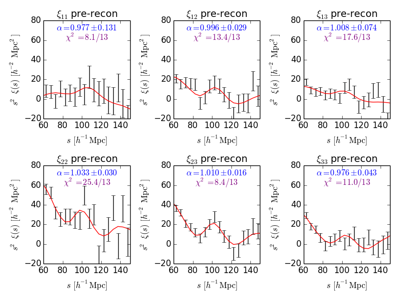
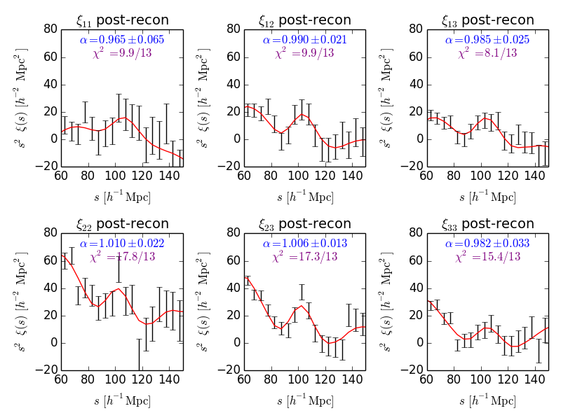
Figure 3: Auto-correlation and cross-correlation function measurements $\xi_{IJ}$ of the CMASS DR12 galaxy dataset in three environmental slices defined by increasing local density. The upper and lower sets of panels display results before and after reconstruction, respectively. The solid line is the best-fitting model in each case, using a template built from the corresponding QPM mock mean correlation function. We also show the $68\%$ confidence range of the posterior probability distribution of $\alpha$, and the $\chi^{2}$ statistic of the best-fitting model and number of degrees of freedom. Baryon acoustic peaks are detected in all six of the post-reconstruction environmental correlation functions.

3 BAO fitting

We considered three different models for the baryon acoustic peak in the environmental and total galaxy correlation functions:

• A model constructed from a theoretical matter power spectrum,

• A model built from the QPM mock galaxy correlation functions,

• A model based on correlation functions of N-body dark matter simulations including and excluding baryon acoustic oscillations.

Each model describes distortions in a template correlation function $\xi_{\rm template}(s)$ using 5 free parameters: a scale distortion parameter $\alpha$, a correlation function amplitude $B^{2}$, and three nuisance parameters $(A_{0},A_{1},A_{2})$ of a polynomial which marginalizes over the smooth shape of the correlation function, ensuring it contributes no information to the scale fits (Anderson et al., 2014). The form of these models is,

$$\xi(s)=B^{2}\xi_{\rm template}(\alpha s)+A_{0}+A_{1}/s+A_{2}/s^{2},$$ (8)

where the construction of $\xi_{\rm template}$ is discussed below. We performed model fits using emcee (Foreman-Mackey et al., 2013), adopting uniform wide priors for the free parameters. We fitted the correlation function measurements in the range $60<s<150\,h^{-1}$Mpc, testing that this choice resulted in fits to the data and mocks with acceptable values of the $\chi^{2}$ statistic, and that our results did not significantly depend on the chosen fitting range.

In our first version of the model, we constructed $\xi_{\rm template}(s)$ following standard methods for fitting the baryon acoustic peak in the angle-averaged total galaxy correlation function (Anderson et al., 2014), using a model power spectrum $P_{\rm mod}(k)$ generated assuming a fiducial cosmology,

$$\xi_{\rm template}(s)=\frac{1}{2\pi^{2}}\int dk\,k^{2}\,P_{\rm mod}(k)\,j_{0}(ks)\,e^{-k^{2}s_{\rm damp}^{2}},$$ (9)

where $j_{0}(x)$ is the zeroth-order spherical Bessel function and $s_{\rm damp}=1\,h^{-1}$Mpc. The model power spectrum in Equation 9 is calculated as,

$$P_{\rm mod}(k)=P_{\rm nw}(k)\left[1+\left(\frac{P_{\rm lin}(k)}{P_{\rm nw}(k)}-1\right)e^{-\frac{1}{2}k^{2}\Sigma_{\rm nl}^{2}}\right],$$ (10)

where $P_{\rm lin}(k)$ is the linear matter power spectrum computed using the CAMB software (Lewis et al., 2000) in the fiducial cosmology, $P_{\rm nw}(k)$ is a model created using the no-wiggles matter power spectrum fitting formulae of Eisenstein & Hu (1998), and $\Sigma_{\rm nl}$ parameterizes the damping of the acoustic peak due to galaxy displacements. Following Anderson et al. (2014), we fixed $\Sigma_{\rm nl}=8.3$ and $4.6\,h^{-1}$Mpc for our fits to the pre-reconstruction and post-reconstruction correlation functions, respectively, noting that these choices (or indeed marginalizing over $\Sigma_{\rm nl}$ as a free parameter) have no significant effect on the results.

The linear power spectrum generated by CAMB may not be an appropriate model for the clustering pattern in an environmental slice, if the density-dependent power spectrum $P(k|\delta)$ has a different shape to the total power spectrum $P(k)$ (Chiang et al., 2014), and in Figure 2 we indeed find that the acoustic peak shape varies with environment. We therefore considered two additional methods for producing the template correlation function $\xi_{\rm template}(s)$ used in Equation 8 to fit the baryon acoustic peak.

In our second model, we constructed the template using the mean correlation functions of the QPM mocks, measured using the same environmental binning as applied to the galaxy data. The environmental dependence of the correlation function shape is therefore included in the fitted templates for this model. We retained free parameters for the correlation function amplitude and polynomial terms, following Equation 8.

We built our third and final model for the acoustic peak from the DEUS N-body dark matter simulations generated from two sets of initial conditions: a linear CAMB power spectrum, and a no-wiggles power spectrum with equivalent cosmological parameters. We measured the correlation functions of these two sets of dark matter particles, $\xi_{\rm wig}(s)$ and $\xi_{\rm nw}(s)$, using the same environmental binning as applied to the galaxy data, and constructed a model correlation function from these measurements as,

$$\xi(s)=B^{2}\left[\xi_{\rm wig}(\alpha s)-\xi_{\rm nw}(\alpha s)\right]+\xi_{\rm nw}(\alpha s)+A_{0}+A_{1}/s+A_{2}/s^{2},$$ (11)

following the form proposed by Kitaura et al. (2016), tested on the correlation function of minima of the density field.

Given that our correlation function templates are generated using a range of model cosmologies with different corresponding standard ruler scales, as summarized in Table 1, we scaled the fitted values of $\alpha$ such that they were all referenced to the fiducial BOSS DR12 cosmology to enable a consistent comparison of results,

$$D_{V}=\alpha\,D_{V,{\rm DR12-fid}},$$ (12)

where $D_{V}$ is the volume-weighted distance measured by BAO in the angle-averaged correlation function, defined in terms of the angular diameter distance $D_{A}(z)$ and Hubble parameter $H(z)$ as,

$$D_{V}(z)=\left[\frac{c\,z\,D_{A}(z)^{2}}{H(z)}\right]^{1/3},$$ (13)

where $c$ is the speed of light and $D_{V,{\rm DR12-fid}}(z=0.57)=2059.6$ Mpc.

Discussing this last point in more detail, suppose that we fit a baryon acoustic peak with observed standard ruler scale $s_{\rm obs}$, using a template correlation function with model standard ruler scale $s_{\rm mod}$, which may differ from the true cosmological standard ruler scale $s_{\rm true}$. Suppose further that we measure the correlation function of the data using a fiducial distance scale $D_{V,{\rm fid}}$, which may differ from the true cosmological distance scale $D_{V,{\rm true}}$. In this case, the Alcock-Paczynski distortion of the scale is given by $s_{\rm obs}=s_{\rm true}\,(D_{V,{\rm fid}}/D_{V,{\rm true}})$, hence the expected best-fitting value of $\alpha$ is,

$$\alpha_{\rm exp}=\frac{s_{\rm mod}}{s_{\rm obs}}=\frac{s_{\rm mod}}{s_{\rm true}}\,\frac{D_{V,{\rm true}}}{D_{V,{\rm fid}}}.$$ (14)

If the template correlation function is calibrated as a function of scale in units of $h^{-1}$Mpc, and if the values of the Hubble parameter are $h_{\rm mod}$ and $h_{\rm fid}$ in the model and fiducial cosmologies respectively, then we obtain,

$$\alpha_{\rm exp}=\frac{s_{\rm mod}[{\rm Mpc}]}{s_{\rm true}[{\rm Mpc}]}\,\frac{D_{V,{\rm true}}[{\rm Mpc}]}{D_{V,{\rm fid}}[{\rm Mpc}]}\,\frac{h_{\rm mod}}{h_{\rm fid}}.$$ (15)

This relation motivates us to calibrate our fitted scale distortion parameters to always refer to the BOSS DR12 fiducial cosmology, as $\alpha_{\rm cal}=\alpha/\alpha_{\rm exp}$. All values of $\alpha$ quoted in the remainder of this paper are values of $\alpha_{\rm cal}$.

In order to check the validity of our fitting procedures, we fitted the QPM mock mean and DEUS correlation functions using all three models described in this section, ensuring that we obtained results consistent with $\alpha_{\rm cal}=1$ after including the appropriate calibration factors discussed above.

4 Results

4.1 BAO fits to the total correlation function

We initially fitted the three models described in Section 3 to the total CMASS galaxy correlation function $\xi_{\rm tot}$ with no environmental binning, before and after density-field reconstruction. Fitting the post-reconstruction correlation function with the CAMB template we obtain $\alpha_{\rm cal}=0.983\pm 0.009$ (referenced to the BOSS DR12 fiducial cosmology), and find that the best-fitting model is a good fit to the data, with a $\chi^{2}$ statistic of $17.8$ for 13 degrees of freedom. The other marginalized measurements of $\alpha_{\rm cal}$ are reported in Table 2.

Table 2: BAO fits to the total correlation function $\xi_{\rm tot}$ of the CMASS DR12 galaxy dataset, and to the auto-correlation and cross-correlation functions $\xi_{IJ}$, in three environmental slices defined by increasing local density. Results are shown before and after density-field reconstruction, comparing models constructed from a CAMB power spectrum, the QPM mock mean, and the DEUS wiggles and no-wiggles dark matter simulations. We report the $68\%$ confidence ranges of the posterior probability distribution for $\alpha_{\rm cal}$ (referenced to the BOSS DR12 fiducial cosmology), together with the $\chi^{2}$ statistic of the best-fitting model and the number of degrees of freedom.

Recon	Data	Template	$\alpha_{\rm cal}$	$\chi^{2}$/dof
Pre-recon	$\xi_{\rm tot}$	CAMB	$0.997\pm 0.013$	$15.1/13$
		QPM mock	$0.992\pm 0.014$	$15.7/13$
		Wig/no-wig sim	$0.990\pm 0.012$	$13.9/13$
Post-recon	$\xi_{\rm tot}$	CAMB	$0.983\pm 0.009$	$17.8/13$
		QPM mock	$0.981\pm 0.008$	$16.6/13$
		Wig/no-wig sim	$0.984\pm 0.009$	$18.9/13$
Pre-recon	$\xi_{11}$	CAMB	$0.960\pm 0.135$	$7.9/13$
		QPM mock	$0.977\pm 0.131$	$8.1/13$
		Wig/no-wig sim	$0.957\pm 0.125$	$7.9/13$
	$\xi_{12}$	CAMB	$1.035\pm 0.063$	$16.4/13$
		QPM mock	$0.996\pm 0.029$	$13.4/13$
		Wig/no-wig sim	$0.974\pm 0.026$	$12.5/13$
	$\xi_{13}$	CAMB	$0.951\pm 0.109$	$17.2/13$
		QPM mock	$1.008\pm 0.074$	$17.6/13$
		Wig/no-wig sim	$0.986\pm 0.055$	$16.7/13$
	$\xi_{22}$	CAMB	$1.023\pm 0.035$	$28.2/13$
		QPM mock	$1.033\pm 0.030$	$25.4/13$
		Wig/no-wig sim	$1.016\pm 0.029$	$27.3/13$
	$\xi_{23}$	CAMB	$1.028\pm 0.019$	$11.6/13$
		QPM mock	$1.010\pm 0.016$	$8.4/13$
		Wig/no-wig sim	$0.994\pm 0.014$	$6.5/13$
	$\xi_{33}$	CAMB	$0.971\pm 0.038$	$9.1/13$
		QPM mock	$0.976\pm 0.043$	$11.0/13$
		Wig/no-wig sim	$0.965\pm 0.032$	$11.0/13$
Post-recon	$\xi_{11}$	CAMB	$0.959\pm 0.081$	$10.0/13$
		QPM mock	$0.965\pm 0.065$	$9.9/13$
		Wig/no-wig sim	$0.969\pm 0.057$	$9.4/13$
	$\xi_{12}$	CAMB	$1.006\pm 0.039$	$15.4/13$
		QPM mock	$0.990\pm 0.021$	$9.9/13$
		Wig/no-wig sim	$0.984\pm 0.018$	$7.4/13$
	$\xi_{13}$	CAMB	$0.975\pm 0.033$	$8.4/13$
		QPM mock	$0.985\pm 0.025$	$8.1/13$
		Wig/no-wig sim	$0.986\pm 0.025$	$7.5/13$
	$\xi_{22}$	CAMB	$1.010\pm 0.035$	$21.5/13$
		QPM mock	$1.010\pm 0.022$	$17.8/13$
		Wig/no-wig sim	$1.000\pm 0.024$	$18.9/13$
	$\xi_{23}$	CAMB	$1.013\pm 0.015$	$22.9/13$
		QPM mock	$1.006\pm 0.013$	$17.3/13$
		Wig/no-wig sim	$0.994\pm 0.011$	$12.8/13$
	$\xi_{33}$	CAMB	$0.979\pm 0.046$	$17.5/13$
		QPM mock	$0.982\pm 0.033$	$15.4/13$
		Wig/no-wig sim	$0.976\pm 0.027$	$14.5/13$

We find that the different BAO templates produce consistent distance-scale fits to the whole-sample correlation function (after correction for the varying model cosmologies as described above), and that our results are consistent with those previously reported by the BOSS collaboration. For example, Cuesta et al. (2016) reported a distance measurement $D_{V}(z=0.57)=2028\pm 21$ Mpc using the post-reconstruction isotropic CMASS correlation function of BOSS DR12, compared to our measurement $D_{V}=2025\pm 19$ Mpc.

4.2 Variation of BAO scale with environment

We then fitted the auto-correlation and cross-correlation functions $\xi_{IJ}$ of the CMASS dataset in the three environmental slices defined by local density, before and after density-field reconstruction, using covariance matrices constructed from corresponding correlation functions of the QPM mocks. We report the marginalized measurements of $\alpha_{\rm cal}$ for all these cases in Table 2.

We can successfully detect and fit the baryon acoustic peak for each of the six correlation functions, and the minimum values of the $\chi^{2}$ statistic are consistent with the distribution expected from the number of degrees of freedom if the data is drawn from the model (the $\chi^{2}$ value of the fit to the pre-reconstruction $\xi_{22}$ is high, but consistent with expected statistical fluctuations). The different models produce consistent values of $\alpha_{\rm cal}$. Given that the CAMB power spectrum model may not be applicable to the clustering of environmental slices as discussed in Section 3, we select the model constructed from the QPM mock mean template as our fiducial choice in the following analysis, although the other models produce consistent results.

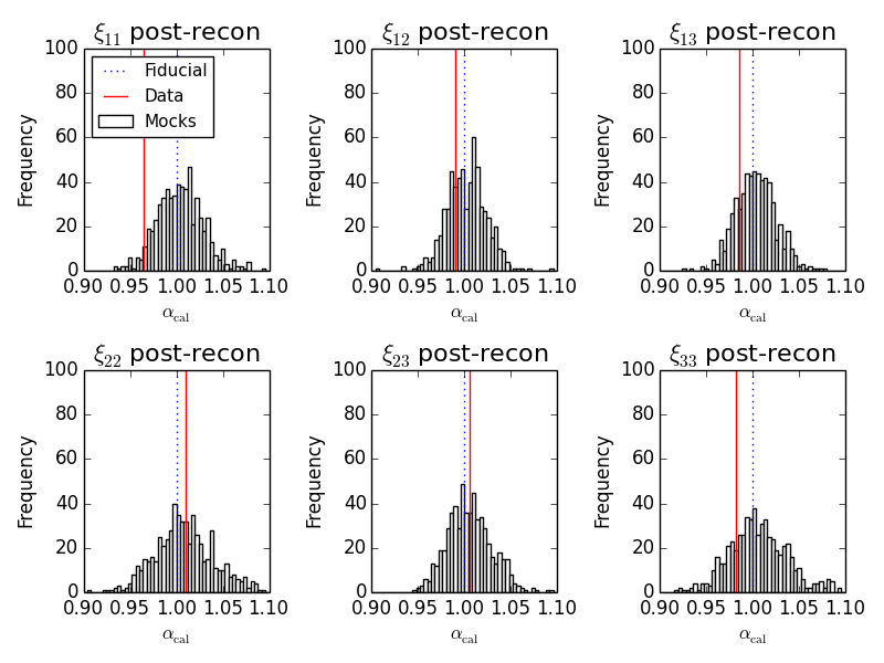
Figure 4: Histogram of best-fitting $\alpha_{\rm cal}$ values fit to the post-reconstruction auto-correlation and cross-correlation functions $\xi_{IJ}$ of each of the 600 QPM mock galaxy catalogues, in three environmental slices defined by increasing local density. The QPM mock mean template is used to construct the BAO model, although the results are not sensitive to this choice. The vertical solid red line illustrates the best-fit to the galaxy data in each case, and the vertical dotted blue line represents the expected fiducial value $\alpha_{\rm cal}=1$ for fits to the mock catalogues using templates built from the mock mean.

We performed corresponding fits to the environmental correlation functions of each of the 600 individual QPM mock catalogues. Figure 4 displays the distribution of best-fitting $\alpha_{\rm cal}$ values across the mocks for each post-reconstruction environmental correlation function $\xi_{IJ}$, superimposing the values obtained from the data, which are consistent with the mock distribution.

Figure 5 compares the values of $\alpha_{\rm cal}$ obtained from each pre-reconstruction and post-reconstruction environmental correlation function, displaying the $68\%$ confidence ranges of the posterior probability distribution for the fit to the data, and the mean and standard deviation of the best-fitting values of $\alpha_{\rm cal}$ across the mock realizations. The values of $\alpha_{\rm cal}$ obtained from different environments are consistent. Fitting a single value of $\alpha_{\rm cal}$ to the six individual post-reconstruction measurements (pre-reconstruction results are given in brackets), using a covariance matrix of $\alpha_{\rm cal}$ values deduced from the QPM mock catalogues, we find $\alpha_{\rm cal}=0.987\pm 0.011$ ($0.997\pm 0.016$) with a minimum $\chi^{2}=1.6$ ($1.4$) for 5 degrees of freedom (six $\alpha_{\rm cal}$ measurements minus one fitted parameter). These results are based on the BAO model constructed from the QPM mock mean correlation function in each environment, although the same conclusion holds when using the same CAMB model template to fit each environment.

The measurement of $\alpha_{\rm cal}$, produced by combining the values in each environment, is consistent with the fit to the total galaxy correlation function, $\alpha_{\rm cal}=0.984\pm 0.009$ ($0.990\pm 0.012$), albeit with a slightly inflated error. We attribute this increased error to the fact that, although the acoustic peaks in each environmental correlation functions are detectable, they are measured with a poorer statistical significance than for the total correlation function. The error in the distance-scale fit is a sharply decreasing function of BAO detection significance in the regime where the acoustic peak is just being resolved, changing faster than the naive $\sqrt{\rm Volume}$ scaling we may associate with sub-dividing a dataset. Future galaxy redshift surveys will allow acoustic peak detections in different data subsets in the high-significance regime, which may allow an improvement in the BAO fitting from sub-division into environments to be realized.

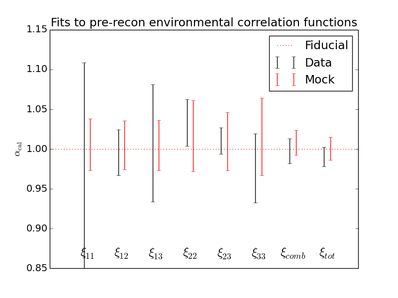
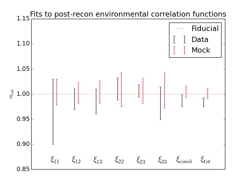
Figure 5: The $68\%$ confidence range of the fits of $\alpha_{\rm cal}$ to the pre-reconstruction (upper panel) and post-reconstruction (lower panel) auto-correlation and cross-correlation function measurements $\xi_{IJ}$ of the CMASS DR12 galaxy dataset, in three environmental slices defined by increasing local density. The mean and standard deviation of the best-fitting values of $\alpha_{\rm cal}$ for the ensemble of QPM mock catalogues are also displayed. The last two pairs of results show the results of fitting a single $\alpha_{\rm cal}$ value to the set of measurements in different environments, including the appropriate covariance ($\xi_{\rm comb}$), and to the total galaxy correlation function ($\xi_{\rm tot}$). These procedures produce similar final results. The QPM mock mean template is used to construct the BAO model, although the results are not sensitive to this choice.

4.3 Variation of the error in the BAO scale with environmental weighting

Finally, we explored the effect on acoustic peak fits of assigning a varying weight with environment when constructing the total galaxy correlation function from the pair counts. This weighting is accomplished by the factor $x$ defined by Equation 2, where $x=-1$ ($+1$) corresponds to assigning double weight to the lowest (highest) density environment, and zero weight to the highest (lowest) density environment. For each new value of $x$, we re-determined the template correlation function (again using the QPM mock mean) and covariance matrix of the measurements by applying the same procedure to the mock catalogues. We note that this analysis uses the original pair counts measured in 12 narrow density bins, and does not use the 3 environmental correlation functions analyzed in the previous section.

Figure 6 presents the $68\%$ error in the fitted distortion scale $\alpha_{\rm cal}$ for the data, and the standard deviation of the best-fitting $\alpha_{\rm cal}$ values for the ensemble of mocks, as a function of the weighting parameter $x$, for the pre-reconstruction and post-reconstruction correlation functions. Using the ensemble of mocks, we find that moderately upweighting underdense environments using $x\approx-0.5$ improves the standard deviation in $\alpha_{\rm cal}$ by $8\%$ (pre-reconstruction, with the scatter improving from $1.45\%$ to $1.34\%$) and $3\%$ (post-reconstruction, $1.03\%$ to $1.00\%$). These results are consistent with the notion that the acoustic peak is somewhat sharper in underdense environments. If the weight of underdense environments is further increased, then the Poisson noise in the correlation function starts to dominate, resulting in poorer measurements.

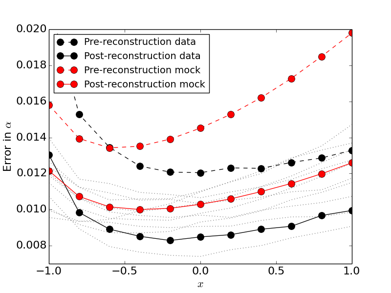
Figure 6: The $68\%$ error in the distortion scale $\alpha_{\rm cal}$ fitted to the data, or the standard deviation of the best-fitting $\alpha_{\rm cal}$ values to the ensemble of mocks, as a function of the parameter $x$ which controls the relative weighting of different environments to the pair count via Equation 2. Results are shown both pre- and post-reconstruction. In order to indicate the effect of sample variance, results are also plotted for the first 10 mocks as the grey dotted lines.

We find that weighting environments does not produce such a strong enhancement in the accuracy of the standard ruler when applied to the data, although a slight ($2\%$) improvement in the error is obtained in the case of the post-reconstruction correlation function for $x=-0.2$, slightly upweighting underdense environments. These results are consistent with the range of behaviours observed in different realizations of the QPM mocks. As an illustration of the sample variance, in Figure 6 we overlay the corresponding trends for each of the first 10 mocks in the post-reconstruction case.

Our conclusions are qualitatively consistent with those reported in a N-body simulation study by Achitouv & Blake (2015), who also found that upweighting underdense regions improves the accuracy of baryon acoustic peak fits by a few per cent for a weighting parameter $x\approx-0.5$. Unlike Achitouv & Blake (2015), our constraints in this study degrade for $x<-0.5$, due to the increased Poisson noise of the CMASS sample. With a higher-density sample, Achitouv & Blake (2015) were able to adopt a smaller smoothing scale more comparable to the halo Lagrangian radii, and apply higher-order corrections to the Zeldovich approximation.

5 Conclusions

The baryon acoustic peak, a robust prediction of early-universe physics, is distorted by the growth of structure in the late-time universe, imprinting additional cosmological information on the feature. We have measured the large-scale clustering properties of the BOSS DR12 CMASS galaxy sample and corresponding mock catalogues, within and between environmental slices defined by the local galaxy overdensity $\delta$ smoothed on $15\,h^{-1}$Mpc scales. Our goal was to delineate the dependence of the baryon acoustic peak scale and shape on environment, and to test if weighting galaxies as a function of environment improved the accuracy of the extracted distance scale. Such enhancements may be possible if the acoustic peak template used in model-fitting, or the accuracy of the displacements inferred by density-field reconstruction, depend on environment.

The CMASS dataset permitted the measurement of baryon acoustic peaks in each of the six auto-correlation and cross-correlation functions of galaxies in three density slices $-1<\delta<0.01$, $0.01<\delta<0.14$ and $\delta>0.14$, where these divisions split the survey into three sub-samples covering volumes in the ratio 7:2:3. Given that a linear power spectrum model may not provide a good description of fluctuations within a slice of environments, we performed acoustic peak fitting using two additional templates constructed as the mean of the corresponding environmental correlations of two mock catalogues: the QPM CMASS mocks, and dark matter N-body simulations constructed from initial conditions including and excluding baryon acoustic oscillations. The mock mean correlation functions reveal that the acoustic peak shape depends on environment, both before and after density-field reconstruction, although the peak scale does not.

The standard-ruler scales fitted to the correlation functions assuming these different templates are in close agreement, and the best-fitting distances are consistent between the environments. Fitting a single distance scale across all the environments, with appropriate covariance, we obtain a combined fit which is close to the result of fitting the total correlation function, albeit with a $\sim 20\%$ greater distance error. We attribute the somewhat larger error to the reduced significance of the acoustic peak detections for individual environments.

Assigning galaxies in underdense environments moderately higher weights when measuring the total correlation function of the sample lowers the scatter in the best-fitting distance scales by a few per cent for the ensemble of QPM mocks, both before and after density-field reconstruction. Specifically, by up-weighting underdense regions and down-weighting overdense regions by up to $50\%$, the scatter in the preferred-scale fits to the ensemble of mocks improves from $1.45\%$ to $1.34\%$ (pre-reconstruction) and $1.03\%$ to $1.00\%$ (post-reconstruction). This finding is consistent with the broadening of the acoustic peak and reduced accuracy of reconstruction in overdense environments. If the weight of underdense environments is further increased, then the Poisson noise in the correlation function starts to dominate, resulting in poorer measurements. The gains in applying such weights to the DR12 CMASS dataset are not as evident as for the mocks, although the observed trends are consistent with sample variance across the ensemble of mocks.

As prospects for future work, studying perturbation theory models for the environmental correlation function on BAO scales would allow the construction of more accurate theoretical templates for BAO fitting to environmental correlation functions, and for the extraction of the other cosmological information encoded in the variation of clustering with environment. Another extension of this work would be to derive the optimal environmental weight, considering both the variation of the acoustic peak shape with environment and Poisson noise. Finally, future large-volume galaxy samples spanning a wider range of environments than Luminous Red Galaxies, such as the Taipan Galaxy Survey (da Cunha et al., 2017), may allow more significant improvements from environmental weighting.

References

- Achitouv & Blake (2015) Achitouv I., Blake C., 2015, Phys. Rev. D, 92, 083523
- Alam et al. (2017) Alam S., et al., 2017, MNRAS, 470, 2617
- Alimi et al. (2012) Alimi J.-M., et al., 2012, preprint, (arXiv:1206.2838)
- Anderson et al. (2014) Anderson L., et al., 2014, MNRAS, 441, 24
- Astropy Collaboration et al. (2013) Astropy Collaboration et al., 2013, A&A, 558, A33
- Ata et al. (2018) Ata M., et al., 2018, MNRAS, 473, 4773
- Bautista et al. (2017) Bautista J. E., et al., 2017, A&A, 603, A12
- Beutler et al. (2011) Beutler F., et al., 2011, MNRAS, 416, 3017
- Blake & Glazebrook (2003) Blake C., Glazebrook K., 2003, ApJ, 594, 665
- Blake et al. (2011) Blake C., et al., 2011, MNRAS, 418, 1707
- Burden et al. (2015) Burden A., Percival W. J., Howlett C., 2015, MNRAS, 453, 456
- Chiang et al. (2014) Chiang C.-T., Wagner C., Schmidt F., Komatsu E., 2014, J. Cosmology Astropart. Phys., 5, 048
- Crocce & Scoccimarro (2008) Crocce M., Scoccimarro R., 2008, Phys. Rev. D, 77, 023533
- Cuesta et al. (2016) Cuesta A. J., et al., 2016, MNRAS, 457, 1770
- Dawson et al. (2013) Dawson K. S., et al., 2013, AJ, 145, 10
- Eisenstein & Hu (1998) Eisenstein D. J., Hu W., 1998, ApJ, 496, 605
- Eisenstein & White (2004) Eisenstein D., White M., 2004, Phys. Rev. D, 70, 103523
- Eisenstein et al. (1998) Eisenstein D. J., Hu W., Tegmark M., 1998, ApJ, 504, L57
- Eisenstein et al. (2005) Eisenstein D. J., et al., 2005, ApJ, 633, 560
- Eisenstein et al. (2007a) Eisenstein D. J., Seo H.-J., White M., 2007a, ApJ, 664, 660
- Eisenstein et al. (2007b) Eisenstein D. J., Seo H.-J., Sirko E., Spergel D. N., 2007b, ApJ, 664, 675
- Falck et al. (2015) Falck B., Koyama K., Zhao G.-B., 2015, J. Cosmology Astropart. Phys., 7, 049
- Feldman et al. (1994) Feldman H. A., Kaiser N., Peacock J. A., 1994, ApJ, 426, 23
- Foreman-Mackey et al. (2013) Foreman-Mackey D., Hogg D. W., Lang D., Goodman J., 2013, PASP, 125, 306
- Hunter (2007) Hunter J. D., 2007, Computing In Science & Engineering, 9, 90
- Kazin et al. (2014) Kazin E. A., et al., 2014, MNRAS, 441, 3524
- Kitaura et al. (2016) Kitaura F.-S., et al., 2016, Physical Review Letters, 116, 171301
- Landy & Szalay (1993) Landy S. D., Szalay A. S., 1993, ApJ, 412, 64
- Lewis et al. (2000) Lewis A., Challinor A., Lasenby A., 2000, ApJ, 538, 473
- Matsubara (2008) Matsubara T., 2008, Phys. Rev. D, 78, 083519
- McCullagh et al. (2013) McCullagh N., Neyrinck M. C., Szapudi I., Szalay A. S., 2013, ApJ, 763, L14
- Neyrinck et al. (2018) Neyrinck M. C., Szapudi I., McCullagh N., Szalay A. S., Falck B., Wang J., 2018, MNRAS, 478, 2495
- Padmanabhan et al. (2009) Padmanabhan N., White M., Cohn J. D., 2009, Phys. Rev. D, 79, 063523
- Padmanabhan et al. (2012) Padmanabhan N., Xu X., Eisenstein D. J., Scalzo R., Cuesta A. J., Mehta K. T., Kazin E., 2012, MNRAS, 427, 2132
- Planck Collaboration et al. (2018) Planck Collaboration et al., 2018, preprint, (arXiv:1807.06205)
- Rasera et al. (2014) Rasera Y., Corasaniti P.-S., Alimi J.-M., Bouillot V., Reverdy V., Balmès I., 2014, MNRAS, 440, 1420
- Reid et al. (2016) Reid B., et al., 2016, MNRAS, 455, 1553
- Ross et al. (2015) Ross A. J., Samushia L., Howlett C., Percival W. J., Burden A., Manera M., 2015, MNRAS, 449, 835
- Roukema et al. (2015) Roukema B. F., Buchert T., Ostrowski J. J., France M. J., 2015, MNRAS, 448, 1660
- Roukema et al. (2016) Roukema B. F., Buchert T., Fujii H., Ostrowski J. J., 2016, MNRAS, 456, L45
- Seo & Eisenstein (2003) Seo H.-J., Eisenstein D. J., 2003, ApJ, 598, 720
- Seo et al. (2008) Seo H.-J., Siegel E. R., Eisenstein D. J., White M., 2008, ApJ, 686, 13
- Sherwin & Zaldarriaga (2012) Sherwin B. D., Zaldarriaga M., 2012, Phys. Rev. D, 85, 103523
- Sinha (2016) Sinha M., 2016, Corrfunc: Corrfunc-1.1.0, doi:10.5281/zenodo.55161, http://dx.doi.org/10.5281/zenodo.55161
- Smith et al. (2008) Smith R. E., Scoccimarro R., Sheth R. K., 2008, Phys. Rev. D, 77, 043525
- Vargas-Magaña et al. (2017) Vargas-Magaña M., Ho S., Fromenteau S., Cuesta A. J., 2017, MNRAS, 467, 2331
- White (2016) White M., 2016, J. Cosmology Astropart. Phys., 11, 057
- White et al. (2014) White M., Tinker J. L., McBride C. K., 2014, MNRAS, 437, 2594
- Zhao et al. (2018) Zhao C., Chuang C.-H., Liang Y., Kitaura F.-S., Vargas-Magaña M., Tao C., Pellejero-Ibanez M., Yepes G., 2018, preprint, (arXiv:1802.03990)
- da Cunha et al. (2017) da Cunha E., et al., 2017, Publ. Astron. Soc. Australia, 34, e047