Lidar Measurement Bias Estimation via Return Waveform Modelling in a Context of 3D Mapping

Abstract

In a context of 3D mapping, it is very important to obtain accurate measurements from sensors. In particular, Light Detection And Ranging (LIDAR) measurements are typically treated as a zero-mean Gaussian distribution. We show that this assumption leads to predictable localisation drifts, especially when a bias related to measuring obstacles with high incidence angles is not taken into consideration. Moreover, we present a way to physically understand and model this bias, which generalizes to multiple sensors. Using an experimental setup, we measured the bias of the Sick LMS151, Velodyne HDL-32E, and Robosense RS-LiDAR-16 as a function of depth and incidence angle, and showed that the bias can reach $20\text{\,}\mathrm{cm}$ for high incidence angles. We then used our model to remove the bias from the measurements, leading to more accurate maps and a reduced localisation drift.

I Introduction

LIDAR have become widespread in robotics to produce increasingly precise maps of the environment. As every sensor, LIDAR suffer from noise, directly impacting the quality of maps. In particular, we observed that the incidence angle of the laser beam can cause significant errors in mapping algorithms.

For example, when a map of the environment is produced in a tunnel or a hallway, notable errors occur in the distance where the incidence angle is very important. The error can be a simple zero-mean noise. However, it is possible that the noise is not truly centred on zero, hence has a bias. Figure 1 shows a map taken from a straight underground tunnel, produced with the LMS151. Although the tunnel is known to be straight, the produced map tends to bend at large distances. Moreover, the tunnel bends in a preferred direction depending on which wall the LIDAR is closest. This deformation is repeatable given a trajectory, which disproves the idea that the bending is only induced by the integration of a zero-mean noise. This observation leads to the hypothesis that LIDAR have a bias that depends on the distance and the incidence angle.

Figure 1: Impact of bias from LIDAR measurements on mapping. The map is bending depending on which wall the robot was closest to while driving. Coloured arrows represent the starting position of the robot and the wall it followed (blue: left; cyan: right). Once the bias is taken into consideration, the map (red) drifts significantly less. Note that the scale on the length of the corridor was changed to highlight the impact of the bias. The corridor is 47 times longer than its width.

Modelling this bias would correct the measurements and improve the map quality. Figure 1 shows the unbent map, where the bias was removed from the LIDAR measurements.

The contribution of this paper is a physical explanation for the bias, as well as a way to quantify and correct this bias for common LIDAR used in mobile robotics. Section II presents a survey of the modelisation of the noise of LIDAR, often considered as a zero-mean white noise. Section III describes the modelisation of the return waveform. We test our hypothesis in Section IV with an experimental setup for the LIDAR Sick LMS151, Velodyne HDL-32E, and the new Robosense RS-LiDAR-16 (characterised in [1]), leading to a novel method to correct the measurements of LIDAR whose results are presented in Section V.

II Related Works

In the literature, many have shown the relationship between the noise of LIDAR measurements and the incidence angle. An extensive study of the influence of the incidence angle on the measurements was conducted in [2, 3, 4]. The authors focused on the propagation of the noise induced by the incidence angle, albeit assuming no bias. [5] created a probabilistic model of LIDAR and found that the behaviour of the Hokuyo UTM-30LX at high incidence angles is different from normal distributions. They discovered a bias at high incidence angles but mainly because the beam was close to a corner, hence measuring the reflexivity of the laser beam and not the bias itself. [6] analysed the noise from several surfaces and stated that standard models for LIDAR (i.e., without bias) overestimate the variance to cope with unmodelled biases. Our hypothesis is reinforced by [7], who characterised the bias of the Sick LMS-200 as a function of the incidence angle and the depth and then integrated it to their mapping algorithm. They modelled the bias using an empirical function and concluded that the contribution of the correction is negligible in their environment, which had many features and landmarks. In this paper, we demonstrate that the contribution of the bias for the 2D and 3D cases is not negligible in all environments.

LIDAR were characterised as a function of many factors, such as depth, internal temperature or incidence angle. [8] showed that the target seems to move away from the sensor as the incidence angle increases. [9] characterised the Sick LMS200 using an experimental setup similar to the one used in the present article and concluded that the incidence angle has a great influence on the reading. They did not model the error as a function of the incidence angle as they stated that this information is not usually known in most mobile robotics applications. It is nowadays possible to estimate this parameter, which is done in this article. The same experimental setup was used by [10] to characterise the Hokuyo URG-04LX, but the authors were not able to obtain reliable measurements for an incidence angle greater than $40\text{\,}\mathrm{\SIUnitSymbolDegree}$. They therefore could not observe the bias, which manifests itself at high incidence angles. [11] studied the performances of the Velodyne VLP-16 at different incidence angles, highlighting the bias induced by it. They gave a partial estimate of the bias but were unable to connect it with a physical phenomenon, leading to large unmodelled errors. At a larger scale, [12] conducted an analysis of the influence of terrestrial laser scanning for tunnel inspection, and modelled the error as a function of the incidence angle and the depth with a non-parametric kernel smoother. Nevertheless, this provides no physical explanation of the bias. This last solution is sensitive to the density of the experimental characterisation, which could be simplified using an analytic solution.

LIDAR were also modelled and integrated in simulation softwares. [13] and [14] modelled a LIDAR return waveform using a Gaussian beam representation to compute the laser beam propagation. They however did not consider the incidence angle. Our work extends these simulations by considering it. [15] modelled further the return waveform by taking into account the electronics of the sensor and the discrimination method used to find the maximum of the return waveform. Our method differs from the last one as [15] discretises the laser beam, mainly to handle the mixed pixel problem [16]. Finally, [17] concluded that the study of the full return waveform leads to better results than using an electronic peak detector to estimate the distance. This statement supports our theory that the current detectors embedded in LIDAR cannot handle all of the situations the beams can encounter.

III Modelling of the Waveform

A first intuition of the phenomenon is illustrated in Figure 2. When the laser beam hits an oriented surface, the energy distribution is not uniform. A great amount of intensity returns sooner to the sensor than if the surface was not oriented. This means that the return waveform will have a different shape depending on the incidence angle, inducing a bias in the measurement.

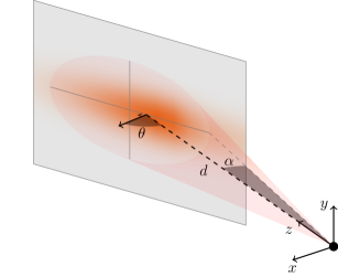
Figure 2: Illustration of a single laser beam (shaded in red), with an aperture half-angle $\alpha$, hitting an oriented surface of $\theta$ degrees at a distance $d$. The bias comes from the intensity distribution being skewed causing the peak of intensity to be detected sooner once integrated by the receptor.

We simulate the return waveform of a LIDAR using a four-step process. (1) A pulse of light is emitted, going through the lens of the LIDAR. (2) The beam is then projected onto the oriented plane. (3) The beam is reflected. (4) The light comes back to the LIDAR as a function of time, taking into account that the travel time for a given point on the plane differs according to its position.

Without loss of generality, we place the sensor at the origin, facing the $\vec{z}$ axis. The plane is parallel to the $\vec{y}$ axis and its normal forms an angle $\theta$ with the $\vec{z}$ axis. Figure 3 summarises the notations for the 2D case.

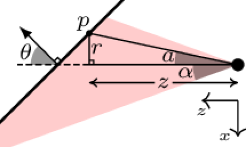
Figure 3: Notations for the 2D case. Each point $p$ on the plane is defined as a function of $a$, the angle formed with the centre of the beam. $p$ is at an orthogonal distance $z$ from the LIDAR and at a distance $r$ from the centre of the beam.

We model the emission of the light pulse $\mathrm{P}_{\text{e}}\left(t\right)$ with a Gaussian of length $\tau$ and power $I_{0}$ as done in [15]

$$\mathrm{P}_{\text{e}}\left(t\right)=I_{0}\exp\left({\frac{-t^{2}}{2\sigma^{2}}}\right),$$ (1)

with $\sigma=\frac{\tau}{\sqrt{2\pi}}$. The beam is then projected onto the plane at a distance $d$ and rotated by $\theta\text{\,}\mathrm{\SIUnitSymbolDegree}$. Since we cannot know the reflexivity properties of the plane, we chose to use the Lambertian model $\mathrm{L}(\cdot)$ for the projected energy $\mathrm{P}_{\text{p}}\left(\cdot\right)$, given a known plane, as

$$\mathrm{P}_{\text{p}}\left(t,a,b\,\middle|\,d,\theta\right)=\mathrm{L}(\gamma)\cdot\mathrm{P}_{\text{e}}\left(t-\frac{\rho}{c}\right)\cdot\mathrm{I}(r,z),$$ (2)

with $\mathrm{L}(\gamma)=\cos(\gamma)$, $\gamma=\cos^{-1}(\cos(a+\theta)\cos b)$, $c$ the speed of light, $a$ the angle between the point and the centre of the beam along the major axis of the ellipse (i.e., on the plane $\vec{x}\vec{z}$), $b$ the angle between the point and the centre of the beam along the minor axis (i.e., on the plane $\vec{y}\vec{z}$), $r$ the distance from the centre of the beam and $z$ the distance of the centre of the beam from the emitter (Figure 3). The length $\rho$ corresponds to the distance between the emitter and the point and can be computed as follows

$$\rho =\sqrt{\smash[b]{\underbrace{\vphantom{\left(d\frac{\cos(a)\cos(\theta)}{\cos(a+\theta)}\right)^{2}}z^{2}\tan^{2}(a)+z^{2}\tan^{2}(b)}_{r^{2}}}+\smash[b]{\underbrace{\left(d\frac{\cos a\cos\theta}{\cos(a+\theta)}\right)^{2}}_{z^{2}}}}.$$ (3)

Equation 2 also uses the Gaussian beam model $\mathrm{I}(\cdot)$, with a wavelength $\lambda$ and the aperture half-angle $\alpha$, defined as

$$\mathrm{I}\left(r,z\,\middle|\,\lambda,\alpha\right)=\left(\frac{\omega_{0}}{\alpha z}\right)^{2}\cdot\exp\left(\frac{-2r^{2}}{\alpha^{2}z^{2}}\right),$$ (4)

at large distance, with $\omega_{0}=\frac{\lambda}{\pi\alpha}$. The function $\mathrm{I}(\cdot)$ therefore represents the intensity for the points along the basis of a circular cone of radius $r$ and height $z$.

The beam is then returned to the sensor. To determine the total energy returned to the detector $\mathrm{P}_{\text{r}}\left(\cdot\right)$, we need to integrate over the surface (i.e., in both directions) of the plane at each time $t$, leading to

$$\mathrm{P}_{\text{r}}\left(t\,\middle|\,d,\theta\right)=\int_{-\frac{\pi}{2}}^{+\frac{\pi}{2}}\int_{-\frac{\pi}{2}}^{+\frac{\pi}{2}}\mathrm{P}_{\text{p}}\left(t-\frac{\rho}{c},a,b\,\middle|\,d,\theta\right)\operatorname{d\!}b\operatorname{d\!}a,$$ (5)

Figure 4 gives an example of the simulation of the return waveform $\mathrm{P}_{\text{r}}\left(\cdot\right)$ for two different angles of incidence. The shape of the return waveform tends to skew as the incidence angle grows, moving the peak of intensity by $\Delta t$ (i.e., leading to a bias in the measurement).

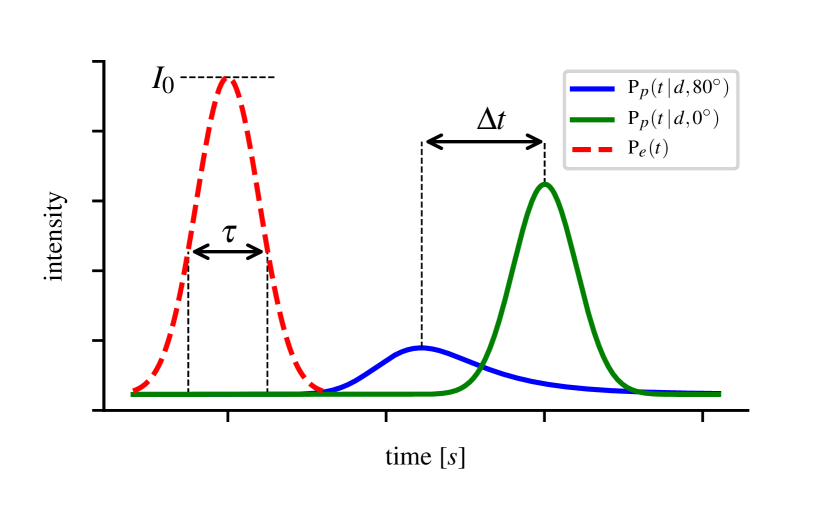
Figure 4: Illustration of two return waveforms hitting a surface at the same distance. In red, the emitted waveform with power $I_{0}$ and length $\tau$. In green, the return waveform with $\theta=$0\text{\,}\mathrm{\SIUnitSymbolDegree}$$. In blue, the return waveform with $\theta=$80\text{\,}\mathrm{\SIUnitSymbolDegree}$$. The peaks of intensity are spaced apart of $\Delta t\text{\,}\mathrm{s}$. The curves also differ in shape, with the waveforms flattening as the incidence angle grows.

One can easily notice that the equation for the return waveform is not computational-friendly. In order to find a closed-form of Equation 5, we restrict the simulation to the 2D case (i.e., keep $b=0$), therefore having only one integral to cope with. This approximation can be made because the distribution of intensity along the $\vec{y}$ axis is not skewed, therefore inducing no further bias (Figure 2). We also bound the integral using the aperture half-angle $\alpha$. The intensity is indeed negligible outside these boundaries. We obtain

$$\mathrm{P}_{\text{r}}\left(t\,\middle|\,d,\theta\right)\approx\int_{-\alpha}^{+\alpha}\mathrm{P}_{\text{p}}\left(t-\frac{\rho}{c},a,0\,\middle|\,d,\theta\right)\operatorname{d\!}a.$$ (6)

Using first-order Taylor series, we find

$$\mathrm{P}_{\text{r}}\left(t\,\middle|\,d,\theta\right)\approx I_{0}\left(\frac{w_{0}}{\alpha d\cos(\theta)}\right)^{2}\exp\left(C\right)\int_{-\alpha}^{+\alpha}f(a)\operatorname{d\!}a,$$ (7)

with $f(a)=(K_{1}-aK_{2})\exp(-Aa^{2}+Ba)$ and

$$A =\frac{2d^{2}\tan^{2}(\theta)}{\sigma^{2}c^{2}}+\frac{2}{\alpha^{2}}, K_{1} =\cos^{3}(\theta),$$

$$B =\frac{1}{\sigma^{2}}\left(t-\frac{2d}{c}\right)\left(\frac{2d\tan(\theta)}{c}\right), K_{2} =3\cos^{2}(\theta)\sin(\theta),$$

$$C =-\frac{1}{2\sigma^{2}}\left(t-\frac{2d}{c}\right)^{2},$$ (8)

which has a closed-form. We will now concentrate on the peak of $\mathrm{P}_{\text{r}}\left(t\,\middle|\,d,\theta\right)$, hence when $t$ is in the neighbourhood of $\frac{2d}{c}$ (where the peak should be if $\theta$ was null). Under this assumption, we can simplify the above equation using again first-order Taylor series. Using $T=t-\frac{2d}{c}$, we express $\mathrm{P}_{\text{r}}\left(\cdot\right)$ as

$$\mathrm{P}_{\text{r}}\left(t\,\middle|\,d,\theta\right)\approx \sum_{i=0}^{3}a_{i}T^{i},$$ (9)

with

$$a_{0} =2AK_{1}L_{1},$$

$$a_{1} =-\frac{2d\tan(\theta)\left(-2L_{2}\alpha\exp\left(-A\alpha^{2}\right)+L_{1}K_{2}\right)}{\sigma^{2}c},$$

$$a_{2} =-\frac{2AK_{1}L_{1}\left(\sigma^{2}c^{2}A\cos^{2}(\theta)+2d^{2}\cos^{2}(\theta)-2d^{2}\right)}{2\cos^{2}(\theta)\sigma^{4}c^{2}A},$$

$$a_{3} =\frac{L_{1}K_{2}d\tan(\theta)\left(\sigma^{2}c^{2}A-2d^{2}\tan^{2}(\theta)\right)}{\sigma^{6}c^{3}A},$$ (10)

$$L_{1} =I_{0}\cdot\left(\frac{w_{0}}{\alpha d\cos(\theta)}\right)^{2}\cdot\frac{\sqrt{\pi}\operatorname{erf}\left(\alpha\sqrt{A}\right)}{2A^{3/2}},$$

$$L_{2} =I_{0}\cdot\left(\frac{w_{0}}{\alpha d\cos(\theta)}\right)^{2}\cdot\frac{K_{2}}{2A}.$$

At this point, we have a function depending on three variables: $d$, $\theta$ and $t$. We need to eliminate the third variable, by defining some metrics on $\mathrm{P}_{\text{r}}\left(t\,\middle|\,d,\theta\right)$. The most logical is the difference of distance the LIDAR would return between the waveforms at $0\text{\,}\mathrm{\SIUnitSymbolDegree}$ and $\theta\text{\,}\mathrm{\SIUnitSymbolDegree}$, if the electronics was able to detect without error the maximum of intensity:

$$\Delta_{d}(d,\theta) =[\operatorname*{arg\,max}_{t}\mathrm{P}_{\text{r}}\left(t\,\middle|\,d,\theta\right)]\cdot\frac{c}{2}-d$$ (11)

$$=\frac{-2a_{2}-\sqrt{4{a_{2}}^{2}-12a_{1}a_{3}}}{6a_{3}}\cdot\frac{c}{2}$$

However, [17] showed that no detector is perfect and that an error is always made. We therefore define another metric to measure the difference of shape between the waveforms at $0\text{\,}\mathrm{\SIUnitSymbolDegree}$ and $\theta\text{\,}\mathrm{\SIUnitSymbolDegree}$:

$$\Delta_{\textrm{shape}}(d,\theta) =1-\frac{\kappa(d,0)}{\kappa(d,\theta)}$$ (12)

with

$$\kappa(d,\theta) =\sqrt{4{a_{2}}^{2}-12a_{1}a_{3}},$$ (13)

the curvature of the return waveform at its peak.

Because of the many uncertainties on the variables and the model which we restricted to the 2D case, we allow our model to have two scaling factors $(s_{1},s_{2})$. The error of distance is then expressed as

$$e(d,\theta)=s_{1}\cdot\Delta_{d}(d,\theta)+s_{2}\cdot\Delta_{\mathrm{shape}}(d,\theta).$$ (14)

These scaling factors will be adjusted for each sensor.

IV Experimental Setup

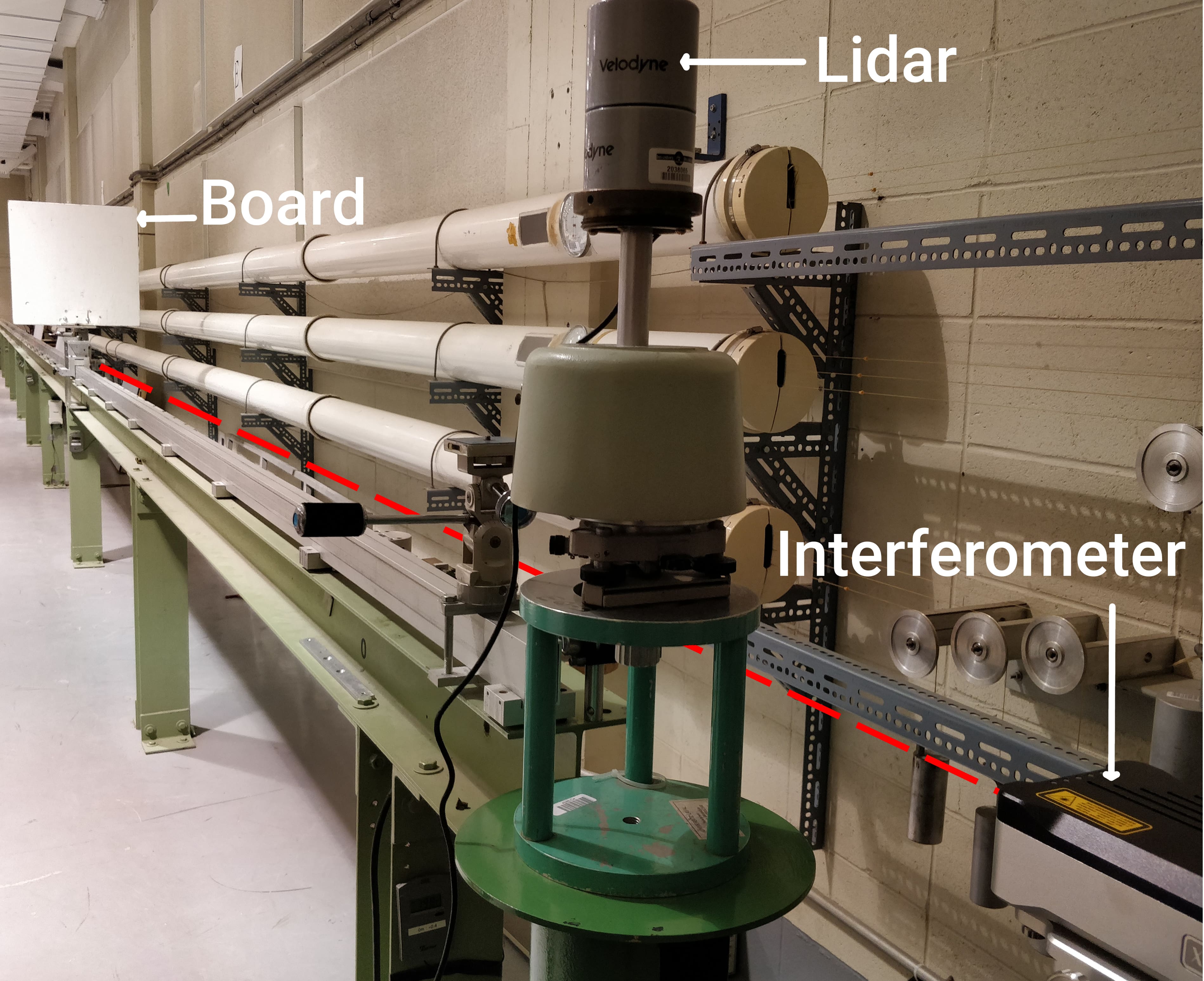
Figure 5: Experimental setup. The LIDAR central beam measures the board which can be rotated gradually. The whole setup is mounted onto a linear motion table, allowing measurements to be made at several distances. The interferometer measures the distance of the board, with its beam indicated with a red dashed-line.

In order to test our hypothesis, we used an experimental setup very similar to the one in [9], as shown in Figure 5. A wooden board of $0.6\times 0.6\text{\,}\mathrm{m}$ was mounted onto a linear motion table (i.e., a rail) of approximately $30\text{\,}\mathrm{m}$. The board can rotate using a graduated disc.

An interferometer (Renishaw XL-80) gives the ground truth distance $D$ between the board and the LIDAR, with an accuracy of the order of $1\text{\,}\mathrm{\SIUnitSymbolMicro m}$. The LIDAR itself is rigidly fixed with respect to the linear motion table with its centre beam aligned with the rail, measuring a distance $d$.

As it can be seen in Figure 6, several parameters need to be adjusted before any measurement. First, the error of orientation $\epsilon_{y}$ of the sensor was cancelled by aiming the LIDAR beam at a very thin object ($5\text{\,}\mathrm{cm}$) on the linear motion table at a large distance (i.e., more than $30\text{\,}\mathrm{m}$). Second, the displacement $\delta_{z}$ between the interferometer and the LIDAR was computed as the mean of the difference of distances returned by the LIDAR and the interferometer with the board at $0\text{\,}\mathrm{\SIUnitSymbolDegree}$. Third, we manually measured the distance $\delta_{\mathcal{C}}$ between the board and its centre of rotation. Finally, we computed the horizontal displacement $\delta_{x}$ by measuring with the LIDAR the distance to the board at different orientations (all below $30\text{\,}\mathrm{\SIUnitSymbolDegree}$, where the bias is assumed to be negligible) and estimated the centre of rotation of the board.

Even if we did our best to minimise these errors, it is very likely that some parameters are not precise enough and could interfere with the measurements. The most important parameter is the rotation $\epsilon_{y}$ of the sensor, which could lead to great errors at high angles and compensate or enhance the studied phenomenon. As validated by [9], we took the mean of the errors at $\theta\text{\,}\mathrm{\SIUnitSymbolDegree}$ and $-\theta\text{\,}\mathrm{\SIUnitSymbolDegree}$ to minimise the influence of $\epsilon_{y}$ and $\delta_{x}$.

Knowing all the parameters, for a distance of measurement $d$ and an incidence angle $\theta$, the corrected distance that the LIDAR should return is

$$D_{c}=D-\delta_{z}+\frac{\delta_{\mathcal{C}}}{\cos(\theta)}-\delta_{x}\tan(\theta).$$ (15)

The error (i.e., bias) is computed as

$$e(d,\theta)=d-D_{c}.$$ (16)

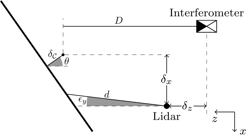
Figure 6: Top-view of the experimental setup. The LIDAR measures the board at a distance $d$ and is misaligned by a small rotation of $\epsilon_{y}$. It is also misplaced from the rail by $\delta_{x}$. The board rotates at a distance $\delta_{\mathcal{C}}$ from its centre of rotation. The interferometer is at a distance $\delta_{z}$ of the LIDAR and measures a distance $D$.

For all three LIDAR, we measured the distance error for twelve orientations of the board. We used steps of $10\text{\,}\mathrm{\SIUnitSymbolDegree}$ from $0\text{\,}\mathrm{\SIUnitSymbolDegree}$ to $60\text{\,}\mathrm{\SIUnitSymbolDegree}$ and steps of $5\text{\,}\mathrm{\SIUnitSymbolDegree}$ from $65\text{\,}\mathrm{\SIUnitSymbolDegree}$ to $85\text{\,}\mathrm{\SIUnitSymbolDegree}$ to increase the resolution at high incidence angles. As for the depth, we used $d\in\{1,2,2.5,3,4,5,7,10\}$ meters. Measurements greater than $10\text{\,}\mathrm{m}$ were unreliable since the beam becomes larger than the board for high orientations of the board. To avoid bias due to temperature drift [16], sensors were powered at least an hour before recording any data and the metrology room used for the experiment had its temperature controlled at $20\text{\,}\mathrm{\SIUnitSymbolCelsius}$. Moreover, for each tuple $\{\theta,d\}$, 96 in total, 45 seconds of measurements were collected to estimate modes and dispersions.

V Results

An excerpt of the data collected for the LMS151 is shown in Figure 7. We can observe how the depth influences the bias for three incidence angles. The data show that the main trend of the bias seems to be a linear function of the depth. The slope of the curve is nevertheless non-linear and a function of the incidence angle, as we see that the curves differ more between $80\text{\,}\mathrm{\SIUnitSymbolDegree}$ and $85\text{\,}\mathrm{\SIUnitSymbolDegree}$ than between $10\text{\,}\mathrm{\SIUnitSymbolDegree}$ and $80\text{\,}\mathrm{\SIUnitSymbolDegree}$. This means that the bias as a function of the incidence angle has a flat region for small angles and grows very quickly for high angles. Figure 7 also shows that the error can be very large for high incidence angles, increasing to more than $20\text{\,}\mathrm{cm}$ for a distance less than $10\text{\,}\mathrm{m}$. Moreover, some odd measurements were present in the dataset. For example, at $4\text{\,}\mathrm{m}$ in Figure 7, the points deviate a little from the main trend. A similar observation has been found in the HDL-32E data. Our hypothesis is that the sensor electronics adjust themselves when the received intensity becomes too weak.

We fitted the parameters $(s_{1},s_{2})$ of Equation 14 with these data. The parameters $I_{0}$ and $\lambda$ do not influence the metrics. The metrics indeed measure a peak and a ratio of curvature, hence are not influenced by the overall power of the beam. We nevertheless use consistent values for those parameters: $I_{0}=$0.39\text{\,}\mathrm{W}\text{\,}{\mathrm{m}}^{-2}$$ and $\lambda=$905\text{\,}\mathrm{nm}$$. We experimented different values for the parameter $\tau$ and observed that it also does not influence the metrics as long as it does not become too large. We used $\tau=$50\text{\,}\mathrm{ns}$$. Hence, the only parameter which truly impacts the metrics is the aperture half-angle $\alpha$. Table I gives the aperture half-angles as well as the scale parameters found using robust least squares fitting.

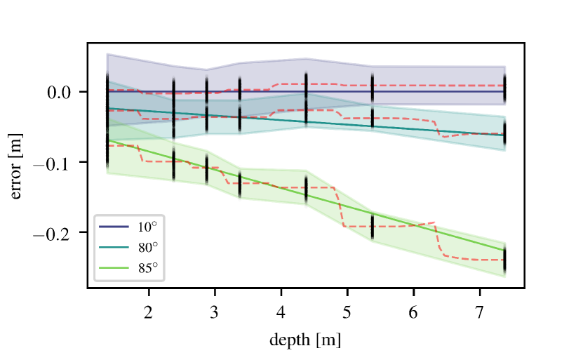
Figure 7: Data collected and fit as a function of the depth for several incidence angles for the LMS151. Raw data are in black and the filled zones represent the variance evaluated at $3\sigma$. In red, the non parametric kernel estimation used in [12] being limited by the sparse data.

TABLE I: Aperture half-angles and scale factors found for each LIDAR

Parameters	LMS151	RS-LiDAR-16	HDL-32E
$\alpha$	$0.43\text{\,}\mathrm{\SIUnitSymbolDegree}$	$0.085\text{\,}\mathrm{\SIUnitSymbolDegree}$	$0.085\text{\,}\mathrm{\SIUnitSymbolDegree}$
$s_{1}$	$6.08$	$84.85$	$10.32$
$s_{2}$	$3.18\text{\times}{10}^{-3}\text{\,}$	$2.14\text{\times}{10}^{-2}\text{\,}$	$7.08\text{\times}{10}^{-3}\text{\,}$

The final results of our correction models are plotted in Figure 8. It is important to note that the bias will always shorten the distance between the sensor and the obstacle. The plots show that the LMS151 and RS-LiDAR-16 are more prone to large errors than the HDL-32E. Our hypothesis is that the electronics are different between the sensors, leading to different biases. The behaviour of the bias also differs between the three sensors: the bias of the LMS151 is very variable as a function of the depth, as opposed to the bias of the HDL-32E which is very stable at constant incidence angles.

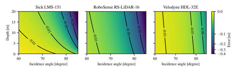
Figure 8: Resulting bias estimations using our analytic model. Isocurves represent the error as a function of depth and incidence angle for each sensor we evaluated (LMS151, RS-LiDAR-16, and HDL-32E). Note that the colours representing the bias are on a logarithmic scale.

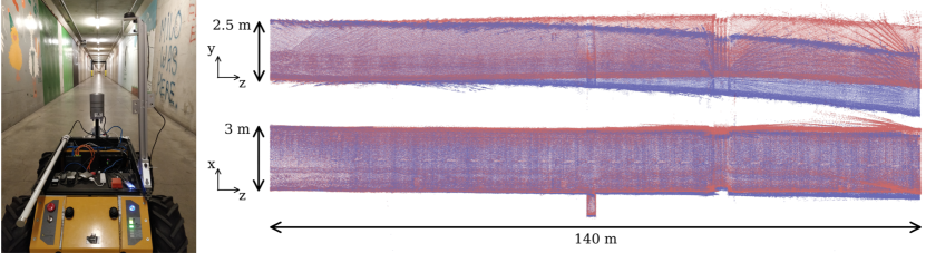
Figure 9: Left: HDL-32E mounted onto the robot in the tunnel. Right: Side view (Top) and top view (Bottom) of the tunnel mapped in 3D. In blue, the map created with the HDL-32E. In red, the map corrected with our method. Although a naive approach was used to compute the surface normals, the map significantly drifts less despite noisy corrections at long ranges (right side of the tunnel). Note that the scale on the length of the corridor was changed to highlight the impact. The corridor is 47 times longer than its width.

We also tested the other models in the literature: [18] chose to remove the points with an incidence angle greater than $65\text{\,}\mathrm{\SIUnitSymbolDegree}$. This choice is a little extreme as it involves removing all the points of the ceiling and the floor for the HDL-32E and RS-LiDAR-16 when mapping a tunnel or corridor, as well as losing the points which are the most constraining in terms of rotation [19]. [7] modelled the bias with an empirical function $c+bd+ae^{k\theta}$. This model does not hold, as it assumes that the slope as a function of the depth is not influenced by the incidence angle, which is shown to be false in Figure 7. The slope at $80\text{\,}\mathrm{\SIUnitSymbolDegree}$ is greater than the slope at $10\text{\,}\mathrm{\SIUnitSymbolDegree}$. Finally, [12] used a non parametric kernel estimation, which is a useful fitting tool but is not connected to a physical explanation of the bias. Figure 7 shows the result of the kernel fitting over our data. A non parametric kernel estimation will always fit the data but needs more samples than an analytic solution. Moreover, it is hard to gather experimental data at large distances (e.g., useful for the HDL-32E and RS-LiDAR-16) and the kernel solution will not extrapolate well.

In order to demonstrate that the bias induces a non negligible deformation of the map, we created a map of an underground tunnel of Laval University with the LMS151 and HDL-32E, shown in Figure 1 and Figure 9. Our correction models are implemented in the libpointmatcher, introduced in [20] and publicly available to the community. Since they rely on a closed-form solution, the computations are lightweight and do not affect the overall performance of the mapping process. Figure 1 shows the result of the correction for a 2D map made with the LMS151. The map is bending according to our position in the corridor. This dependence can be explained as the bias of the LMS151 is highly dependent on the depth. For the incidence angle, the points on the farthest side will have a greater distance, hence a greater bias. Since the bias shortens the distance, the map will bend to the side of the closest wall. Figure 9 shows the result with the HDL-32E in 3D. The map before correction (in blue) goes down a few meters, which is significant enough that it can be seen with the bare eye if indeed it was true. It does not bend to the left or right, as opposed to the 2D map. It can be explained as the bias does not really depend on the distance (Figure 8). The map bends downward because the floor had higher reflexivity than the ceiling, leading to less perceived points on the floor than on the ceiling (i.e., more biased points were contributing to go down rather than up). One could note some very noisy points on the right side of Figure 9, which were not there before the correction. Indeed, the estimation of the normals can be noisy at large depths given the sparse configuration of the HDL-32E, and a small change in the incidence angle at high angles changes drastically the correction.

VI Conclusion

In this paper, we proposed a physical explanation for the bias induced by incidence angles and depths in LIDAR measurements. An approximated closed-form formula was developed and metrics on the return waveform were introduced to cope with the approximations made and the electronics of the sensors. Three LIDAR (LMS151, HDL-32E, and RS-LiDAR-16) were tested in an experimental setup, and biases were found for each sensor. These biases were demonstrated to increase to $20\text{\,}\mathrm{cm}$ at a distance less than $10\text{\,}\mathrm{m}$ for high incidence angles. Our models were then applied to remove the bias in the measurements of the sensors. We used the unbiased measurements to create more accurate maps and reduce the drift of the localisation. Future works should estimate more robustly the normals with an iterative process where the bias is taken into account. This correction is particularly important for autonomous cars using LIDAR, as most of the points on the road have a large incidence angle.

References

- [1] Zhe Wang et al. “Characterization of a RS-LiDAR for 3D Perception” In arXiv preprint arXiv:1709.07641, 2017
- [2] Sylvie Soudarissanane, Jane Van Ree, Alexander Bucksch and Roderik Lindenbergh “Error budget of terrestrial laser scanning : influence of the incidence angle on the scan quality” In Proceedings 3D-NordOst, 2007, pp. 1–8 DOI: 10.13140/RG.2.1.1877.6404
- [3] S Soudarissanane, R Lindenbergh, M Menenti and P Teunissen “Incidence angle influence on the quality of Terrestrial Laser Scanning points” In ISPRS Laserscanning 2009, 2009, pp. 183 –188 URL: http://www.tlsdatabase.ucalgary.ca/node/284
- [4] Sylvie Soudarissanane, Roderik Lindenbergh, Massimo Menenti and Peter Teunissen “Scanning geometry: Influencing factor on the quality of terrestrial laser scanning points” In ISPRS Journal of Photogrammetry and Remote Sensing 66, 2011, pp. 389–399 DOI: 10.1016/j.isprsjprs.2011.01.005
- [5] Hafiz Iman and Nahrul Khair Alang Md Rashid “Probabilistic model of laser range finder for three dimensional grid cell in close range environment” In IIUM Engineering Journal 17.1, 2016, pp. 63–82
- [6] François Pomerleau et al. “Noise characterization of depth sensors for surface inspections” In 2012 2nd International Conference on Applied Robotics for the Power Industry (CARPI), 2012, pp. 16–21 DOI: 10.1109/CARPI.2012.6473358
- [7] Samuel T Pfister, Kristo L Kriechbaum, Stergios I Roumeliotis and Joel W Burdick “Weighted Range Sensor Matching Algorithms for Mobile Robot Displacement Estimation” In IEEE International Conference on Robotics and Automation
- [8] A. Reina and J. Gonzales “Characterization of a radial laser scanner for mobile robot navigation” In IEEE/RSJ International Conference on Intelligent Robot and Systems. Innovative Robotics for Real-World Applications. IROS ’97 2, 1997, pp. 579–585 DOI: 10.1109/IROS.1997.655070
- [9] Cang Ye and Johann Borenstein “Characterization of a 2D laser scanner for mobile robot obstacle negotiation” In IEEE International Conference on Robotics and Automation 3, 2002, pp. 2512–2518 DOI: 10.1109/ROBOT.2002.1013609
- [10] Yoichi Okubo, Cang Ye and Johann Borenstein “Characterization of the Hokuyo URG-04LX laser rangefinder for mobile robot obstacle negotiation” In Unmanned Systems Technology XI 7332, 2009, pp. 733212 DOI: Artn 733212“nDoi 10.1117/12.818332
- [11] John Kidd, Shachak Pe, Firat Eren and Andrew Armstrong “Performance evaluation of the Velodyne VLP-16 system for surface feature surveying” In Canadian Hydrographic Conference, 2016, pp. 1–10
- [12] Javier Roca-Pardiñas, Ramón Argüelles-Fraga, Francisco De Asís López and Celestino Ordóñez “Analysis of the influence of range and angle of incidence of terrestrial laser scanning measurements on tunnel inspection” In Tunnelling and Underground Space Technology incorporating Trenchless Technology Research 43, 2014, pp. 133–139 DOI: 10.1016/j.tust.2014.04.011
- [13] Ali Adnan Al-Temeemy “The Development of a 3D LADAR Simulator Based on a Fast Target Impulse Response Generation Approach” In 3D Research 8.3, 2017, pp. 31 DOI: 10.1007/s13319-017-0142-y
- [14] S Kruapech and J Widjaja “Laser range finder using Gaussian beam range equation” In Optics and Laser Technology 42.5, 2010, pp. 749–754 URL: http://www.scopus.com/scopus/record/display.url?fedsrfIntegrator=MEKPAPERS-SCOCIT&origin=fedsrf&view=basic&eid=2-s2.0-75749136846papers2://publication/uuid/9B95D5C8-E9F9-4E00-8014-70759C1B1E58
- [15] Scott Budge, Brad Leishman and Robert Pack “Simulation and modeling of return waveforms from a ladar beam footprint in USU LadarSIM” In Laser Radar Technology and Applications XI 6214 SPIE, 2006, pp. 62140N DOI: 10.1117/12.666404
- [16] Martial Hebert and Eric Krotkov “3D measurements from imaging laser radars: how good are they?” In Image and vision computing 10.3 Elsevier, 1992, pp. 170–178
- [17] W. Wagner et al. “From single-pulse to full-waveform airborne laser scanners: potential and practical challenges” In XXth International Society for Photogrammetry and Remote Sensing Congress Technical Commission III, 2004, pp. 201–206 URL: http://www.isprs.org/proceedings/XXXV/congress/comm3/papers/267.pdfpapers2://publication/uuid/2659C6C5-62CD-435D-8A9D-EB99BCA5B361
- [18] Derek D Lichti “Error modelling, calibration and analysis of an AM-CW terrestrial laser scanner system” In ISPRS Journal of Photogrammetry and Remote Sensing 61.5, 2007, pp. 307–324 DOI: 10.1016/j.isprsjprs.2006.10.004
- [19] Tsz Ho Kwok “DNSS: Dual-Normal-Space Sampling for 3-D ICP Registration” In IEEE Transactions on Automation Science and Engineering, 2018, pp. 1–12 DOI: 10.1109/TASE.2018.2802725
- [20] François Pomerleau, Francis Colas, Roland Siegwart and Stéphane Magnenat “Comparing ICP variants on real-world data sets: Open-source library and experimental protocol” In Autonomous Robots 34.3, 2013, pp. 133–148 DOI: 10.1007/s10514-013-9327-2