Transient and persistent particle subdiffusion in a disordered chain coupled to bosons

Abstract

We consider the propagation of a single particle in a random chain, assisted by the coupling to dispersive bosons. Time evolution treated with rate equations for hopping between localized states reveals a qualitative difference between dynamics due to noninteracting bosons and hard-core bosons. In the first case the transient dynamics is subdiffusive, but multi–boson processes allow for long-time normal diffusion, while hard-core effects suppress multi–boson processes leading to persistent subdiffusive transport, consistent with numerical results for a full many-body evolution. In contrast, analogous study for a quasiperiodic potential reveals a stable long-time diffusion.

I Introduction

Single particle (SP) localization in a random potential is a well understood phenomenon since the seminal works of Anderson Anderson (1958) and Mott.Mott (1968a) It has become a novel challenge since the proposal of many-body localization (MBL) Basko et al. (2006); Oganesyan and Huse (2007) which would persist in the presence of particle interaction. Pal and Huse (2010); Žnidarič et al. (2008); Barišić and Prelovšek (2010); Gramsch and Rigol (2012); Serbyn et al. (2013a); Bar Lev and Reichman (2014); Prelovšek and Herbrych (2017); Huse et al. (2013); De Luca and Scardicchio (2013); De Luca et al. (2014); Bardarson et al. (2012); Kjäll et al. (2014); Serbyn et al. (2013b); Huse et al. (2014); Serbyn et al. (2014) As the limiting case for the MBL physics, one can consider a single particle in a disordered system coupled to bosonic (or other) degrees of freedom. This problem has a long history related to the phonon-assisted variable-range hopping.Mott (1968b) However, there is recently an increasing interest due to limitations of the validity of this concept Banerjee and Altman (2016) in disordered lattices and due to its relation to MBL physics,Bar Lev et al. (2015); Kozarzewski et al. (2016); Serbyn et al. (2015); Khemani et al. (2015); Gornyi et al. (2005); Altman and Vosk (2015); Rademaker and Ortuño (2016); Chandran et al. (2015); Ros et al. (2015); Eisert et al. (2015); Sierant et al. (2017); Prelovšek et al. (2018); Abanin et al. (2017, 2015); Ponte et al. (2015); Bordia et al. (2017a); Imbrie et al. ; O’Brien et al. (2016); Inglis and Pollet (2016); Goihl et al. (2018); Mierzejewski et al. (2018); Choi et al. (2016) in particular because of anomalous subdiffusive transport.Bonča and Mierzejewski (2017); Gopalakrishnan et al. (2017); Lemut et al. (2017); Bonča et al. (2018); Bordia et al. (2017b); Lev et al. (2017) In general, the coupling to itinerant (dispersive and non–localized) phonon modes leads to the delocalization of the particle. Mott (1968b); Banerjee and Altman (2016) This has recently been tested both for a particle in one-dimensional (1D) disordered chain, coupled to noninteracting bosons (NB),Bonča et al. (2018) as well as for particle dynamics in a $t$-$J$ chain. Bonča and Mierzejewski (2017); Lemut et al. (2017) The latter case represents the coupling to $S=1/2$ spins, or equivalently hard-core bosons (HCB). On the other hand, localization of bosons modifies the variable-range hopping,Banerjee and Altman (2016) being also the case for coupling to nondispersive phonons Bonča et al. (2018) or to localized spin subsystem.Lemut et al. (2017)

Although the evidence above shows that the SP localization is unstable against the coupling to dispersive bosons or, in general, to a heat bath,Nandkishore and Potter (2014); Nandkishore (2015); Huse et al. (2015) the particle dynamics can still be anomalous. Namely, there are examples and regimes where the transport is subdiffusive, i.e., the d.c. mobility vanishes since the spread at long times behaves as $\sigma^{2}(t)\propto t^{\gamma}$ with $0<\gamma<1$. It has been shown, e.g., that a SP subject to local random noiseGopalakrishnan et al. (2017) can exhibit a long transient subdiffusion before turning into a normal diffusion. Similar transport has been found also for spins on a Hubbard chain with a potential disorderPrelovšek et al. (2016a), originating in a singular distribution of effective exchange couplings.Kozarzewski et al. (2018) Such a Griffiths–type mechanism for subdiffusion has been invoked also for the ergodic side of the 1D Heisenberg model with random magnetic fields,Agarwal et al. (2015); Luitz et al. (2016); Gopalakrishnan et al. (2016); Agarwal et al. (2016); Žnidarič et al. (2016); Luitz and Bar Lev (2016) although some results indicate that this might be a transient feature to normal diffusion.Steinigeweg et al. (2016); Barišić et al. (2016); Prelovšek et al. (2016b)

In this paper we consider the propagation of a SP in a random chain, coupled to dispersive bosons, which can be either NB or HCB, whereby the latter case simulates coupling to spins. We analyze the dynamics in terms of the rate equations for the particle hopping between the Anderson eigenstates. The transition rates are evaluated via the Fermi-golden-rule (FGR), but taking into account the actual Anderson eigenstates and multi-boson processes. Our main result concerns the essential difference between NB and HCB models. In the first case, the long-time limit is shown to be diffusive with $\sigma^{2}\propto t$. Nevertheless the evolution is subdiffusive within the initial time-interval $t<t^{*}$, where $t^{*}$ may be very large depending on disorder and temperature $T$. On the other hand, the HCB reveal persistent $\gamma<1$ for not too weak disorder. Subdiffusion is well resolved also in the numerical evolution of the whole many-body quantum system. Still, we find that the propagation depends on the details of potential distribution. In contrast to the HCB case with random uncorrelated potentials, the quasi-periodic potential (as relevant for actual MBL experiments on cold fermionsSchreiber et al. (2015); Bordia et al. (2016); Lüschen et al. (2017)) induces the diffusion in the long-time limit.

II Model

We study the Anderson model for a SP moving in a 1D random potential and coupled to boson degrees,

$$H = -t_{h}\sum_{i}(c^{\dagger}_{i+1}c_{i}+{\mathrm{h}.c.})+\sum_{i}h_{i}n_{i}+g\sum_{i}n_{i}(a^{\dagger}_{i}+a_{i})$$ (1)

$$+ \omega_{0}\sum_{i}a_{i}^{\dagger}a_{i}-t_{b}\sum_{i}(a_{i+1}^{\dagger}a_{i}+\mathrm{h.c.}),$$

where $n_{i}=c^{\dagger}_{i}c_{i}$ is the local particle number. Bosons with $\omega_{0}>0$ are dispersive due to hopping, $0<t_{b}<\omega_{0}/2$. We consider further on two cases: a) NB with a standard boson Hamiltonian $H_{b}=\sum_{q}\omega_{q}a^{\dagger}_{q}a_{q}$ and $\omega_{q}=\omega_{0}-2t_{b}\cos q$, and b) HCB which have restricted Hilbert space with only two states per site (formally $a_{i}^{\dagger}a_{i}^{\dagger}=a_{i}a_{i}=0$). Effectively, HCB represent a spin $S=1/2$ XY chain (in magnetic field $\omega_{0}>0$) closely related to the low-doping limit of the disordered $t$-$J$ or $U\gg t_{h}$ Hubbard models.Mondaini and Rigol (2015); Prelovšek et al. (2016a); Bonča and Mierzejewski (2017) In the following we put $t_{h}=1$ while the potentials are uncorrelated and uniform with $-W<h_{i}<W$. It makes sense to rewrite Eq. (1) in the Anderson basis,

$$H = H_{\rm SP}+H^{\prime}+H_{b},$$

$$H_{\rm SP} = \sum_{l}\epsilon_{l}\varphi_{l}^{\dagger}\varphi_{l},\quad H^{\prime}=\sum_{ll^{\prime}i}\eta_{ll^{\prime}i}\varphi_{l^{\prime}}^{\dagger}\varphi_{l}(a^{\dagger}_{i}+a_{i}),$$ (2)

where $\varphi_{l}=\sum_{i}\phi_{li}c_{i}$ are operators of Anderson localized states (with real $\phi_{li}$), and $\eta_{ll^{\prime}i}=g\phi_{l^{\prime}i}\phi_{li}$.

III Noninteracting bosons

III.1 Transition rates

In the case of NB we proceed by introducing normal modes,

$$H^{\prime}=\sum_{ll^{\prime}}\varphi_{l^{\prime}}^{\dagger}\varphi_{l}H^{\prime}_{ll^{\prime}},\qquad H^{\prime}_{ll^{\prime}}=\sum_{q}(\eta_{ll^{\prime}q}a^{\dagger}_{q}+\eta^{*}_{ll^{\prime}q}a_{q}),$$ (3)

with $\eta_{ll^{\prime}q}=(g/\sqrt{L})\sum_{i}\mathrm{e}^{-iqi}\eta_{ll^{\prime}i}$. Separating $H^{\prime}$ into the diagonal part $H^{\prime}_{d}$ with $l=l^{\prime}$ and the off–diagonal one, we transform out $H^{\prime}_{d}$ via standard canonical transformation,

$$\tilde{H}=\mathrm{e}^{S}H\mathrm{e}^{-S},\quad S=\sum_{l}n_{l}A_{l},\quad A_{l}=\sum_{k}[\zeta_{lk}a^{\dagger}_{k}-\zeta^{*}_{lk}a_{k}],$$ (4)

with $\zeta_{lk}=\eta_{llk}/\omega_{k}$. This leads to transformed $\tilde{H}^{\prime}$ relevant for transitions

$$\tilde{H}^{\prime}_{ll^{\prime}}=\sum_{q}\mathrm{e}^{-A_{ll^{\prime}}}(\eta_{ll^{\prime}q}a^{\dagger}_{q}+\eta^{*}_{ll^{\prime}q}a_{q}),$$ (5)

with $A_{ll^{\prime}}=A_{l^{\prime}}-A_{l}$. Assuming slow transition rates $\Gamma_{ll^{\prime}}$ between states with $\Delta_{ll^{\prime}}\sim\epsilon_{l^{\prime}}-\epsilon_{l}$, we evaluate them within the FGR,

$$\Gamma_{ll^{\prime}}=\mathrm{Re}\int_{0}^{\infty}dt\mathrm{e}^{-i\Delta_{ll^{\prime}}t}G_{ll^{\prime}}(t),\ G_{ll^{\prime}}(t)=2\langle\tilde{H}^{\prime}_{l^{\prime}l}(t)\tilde{H}^{\prime}_{ll^{\prime}}\rangle,$$ (6)

where averaging is over the (boson) equilibrium at $T>0$. We simplify $G_{ll^{\prime}}(t)$ by neglecting in Eqs. (5),(6) cross-terms between $a_{q}$ and multi-boson $A_{ll^{\prime}}$,

$$G_{ll^{\prime}}(t) = 2\sum_{q}|\eta_{ll^{\prime}q}|^{2}g_{q}(t)R_{ll^{\prime}}(t),\leavevmode\nobreak\ R_{ll^{\prime}}(t)=\mathrm{e}^{[Q_{ll^{\prime}}(t)-Q_{ll^{\prime}}(0)]},$$

$$Q_{ll^{\prime}}(t) = \sum_{k}|\zeta_{ll^{\prime}k}|^{2}g_{k}(t),$$ (7)

$$g_{q}(t) = (\bar{n}_{q}+1)\mathrm{e}^{-i\omega_{q}t}+\bar{n}_{q}\mathrm{e}^{i\omega_{q}t},$$

with $\zeta_{ll^{\prime}k}=\zeta_{l^{\prime}k}-\zeta_{lk}$, and boson equilibrium occupation $\bar{n}_{q}=1/[\mathrm{e}^{\omega_{q}/T}-1]$ .

III.2 Simplified transition rates

The above expressions for $\Gamma_{ll^{\prime}}$ account for the details of the model and are rather complex. However, results may also be explained using more qualitative arguments. The essential ingredients within the FGR are the conservation of energy and the overlaps between eigenstates $\phi_{li},\phi_{l^{\prime}i}$. This suggests a simplified form,

$$\Gamma^{\rm s}_{ll^{\prime}}=B\leavevmode\nobreak\ \theta(\Omega-|\Delta_{ll^{\prime}}|)M_{ll^{\prime}},$$ (8)

where $M_{ll^{\prime}}=\sum_{i}\phi^{2}_{li}\;\phi^{2}_{l^{\prime}i}$ and $\Omega\sim\omega_{0}+2t_{b}$ is the rigid cut–off for single-boson emission/absorption. In order to account for multi–boson processes we can employ the saddle-point approximation (in analogy to Ref. Lenarčič and Prelovšek, 2014) to Eq. (6) and $R_{ll^{\prime}}(t)$, leading to an exponential cut–off

$$\Gamma^{\rm m}_{ll^{\prime}}=C\mathrm{exp}\left[-\frac{a|{\Delta_{ll^{\prime}}}|}{\omega_{0}}\right]M_{ll^{\prime}},\quad a=\ln\frac{\Delta_{ll^{\prime}}}{e\nu\omega_{0}},$$ (9)

with $\nu=(1/L)\sum_{k}|\zeta_{ll^{\prime}k}|^{2}\bar{n}_{k}\sim 2\bar{n}g^{2}\Omega^{2}$, which we simplify further taking $\omega_{0}/a\sim\Omega$.

III.3 Rate equations

Within the FGR particle dynamics can be described via the rate equations for occupations $p_{l}(t)$,

$$dp_{l}/dt=\sum_{l^{\prime}}(\Gamma_{l^{\prime}l}p_{l^{\prime}}-\Gamma_{ll^{\prime}}p_{l}).$$ (10)

In order to have a stationary solution, $p_{l}(t)=p_{l}^{0}$, rates $\Gamma_{ll^{\prime}}$ should follow the detailed balanceBouchaud and Georges (1989) $p_{l}^{0}/p_{l^{\prime}}^{0}=\Gamma_{l^{\prime}l}/\Gamma_{ll^{\prime}}$ for each pair $l,l^{\prime}$. This is satisfied within the form of Eq. (6) since to all orders in coupling $g$ one can show that

$$\Gamma_{l^{\prime}l}/\Gamma_{ll^{\prime}}=(\bar{n}_{q}+1)/\bar{n}_{q}=\mathrm{e}^{\Delta_{ll^{\prime}}/T},$$ (11)

taking into account the energy conservation $\omega_{q}=\Delta_{ll^{\prime}}$, see Eqs. (6),(III.1). Then, at $T>0$ we obtain Boltzmann stationary state $p_{l}^{0}=c\leavevmode\nobreak\ \mathrm{e}^{-\epsilon_{l}/T}$ while Eqs. (10) can be symmetrized by introducing,

$$p_{l}(t)=\sqrt{p_{l}^{0}}\tilde{p}_{l}(t),\qquad\tilde{\Gamma}_{l^{\prime}l}=\sqrt{p^{0}_{l^{\prime}}/p^{0}_{l}}\Gamma_{l^{\prime}l}.$$ (12)

The solution of Eq. (10) can be generally represented in the form $p_{l}(t)=\sum_{m}b_{m}p_{ml}\mathrm{e}^{-\Lambda_{m}t}$ with real and nonnegative $\Lambda_{m}$ due to the symmetric $\tilde{\Gamma}_{l^{\prime}l}$, with $p_{ml}$ being corresponding eigenvectors, as well as with the lowest $\Lambda_{1}=0$. Further on, we study dynamical solutions for a particle starting from a single Anderson state, i.e. $p_{l}(0)=\delta_{l,l_{0}}$.

III.4 Results

General characteristics of dynamical solutions can be extracted from $\Gamma_{l^{\prime}l}$, in particular from the distribution of the total local transition rates $\Gamma_{l}=\sum_{l^{\prime}\neq l}\Gamma_{l^{\prime}l}$.Bouchaud and Georges (1989) In the following we calculate the probability distribution ${\cal D}(\Gamma_{l})$ for $\omega_{0}=g=1,t_{b}=0.4$ on chain with $L=200-500$ sites. After finding numerically SP states $\phi_{li}$, we evaluate all $\Gamma_{ll^{\prime}}$ at chosen $T>0$, averaging also over $N_{s}\gg 1$ realizations of disorder. Results presented for integrated distribution

$$I(\Gamma_{l})=\int_{0}^{\Gamma}{\cal D}(\Gamma_{l})d\Gamma_{l}$$ (13)

are shown (in log-log scale) in Fig. 1a for $T=2$ and various disorders, ranging from weak $W=2$ to strong $W=8$. For comparison, we display also corresponding results for simplified rates, Eq. (9), for the same $W$ but adapted $C=6$, which, however, doesn’t affect the structure of ${\cal D}(\Gamma_{l})$. It is meaningful to interpret results in Fig. 1a in terms of power-laws, i.e.,

$$I(\Gamma_{l})\propto\Gamma_{l}^{\alpha},\qquad{\cal D}(\Gamma_{l})\propto\Gamma_{l}^{\alpha-1}.$$ (14)

The corresponding distribution ${\cal F}(\tau_{l})$ for the local lifetimes $\tau_{l}=1/\Gamma_{l}$ can be obtained by comparing $I(\Gamma_{l})=\int_{1/\Gamma_{l}}^{\infty}{\mathrm{d}}\tau_{l}{\cal F}(\tau_{l})$, leading to ${\cal F}(\tau_{l})\propto\tau_{l}^{-(\alpha+1)}$. Results for $I(\Gamma_{l})$ will be further related to the straightforward calculation of the SP spread $\sigma^{2}(t)=\sum_{l}(l-l_{0})^{2}p_{l}(t)$ presented in Fig. 1c for the same parameters.

Different regimes in Fig. 1a can be analyzed in terms of the classical random-trap model.Machta (1985); Bouchaud and Georges (1989) Normal diffusion is the solution for $\alpha>1$ leading to a finite average local lifetime

$$\bar{\tau}=\int_{\tau_{\rm min}}^{\infty}d\tau_{l}\;\tau_{l}{\cal F}(\tau_{l})<\infty,$$ (15)

and $\gamma=1$, i.e., the spread $\sigma^{2}(t)\propto Dt$ with the diffusion constant $D\propto 1/\bar{\tau}$. In Figs. 1a and 1c this is the case for $W<W^{*}\sim 4$, although quite long times $t\gg 100$ are needed to confirm $\gamma\sim 1$.

Here, we are mostly interested in the anomalous subdiffusive dynamics, which is the case for $0<\alpha<1$. If valid in the whole regime $\Gamma_{l}\to 0$ (or equivalently for $\tau_{l}\to\infty$ ) this would imply infinite $\bar{\tau}$. We note that in Fig. 1a, $\alpha<1$ appears for $W>W^{*}$ within large span of $\Gamma_{l}>\Gamma^{*}$. Threshold rate $\Gamma^{*}$ strongly decreases with $W$ and for $W>8$ it is below the numerical accuracy of the present calculations. Nevertheless, for $\Gamma_{l}<\Gamma^{*}$ we observe $\alpha>1$. Therefore $\bar{\tau}$ is huge but finite, suggesting that the subdiffusion is a transient phenomenon and the dynamics should eventually become normal diffusive. In Fig. 1c it is visible that subdiffusive $\gamma<1$ indeed appears for $W>W^{*}$. Still, the normal diffusion may be visible only for long chains $L>1/I(\Gamma^{*})$ and very long times $t\gg\bar{\tau}>1/\Gamma^{*}$.

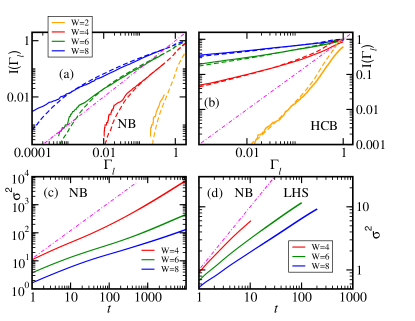
Figure 1: a) and b): Integrated distributions of local rates $I(\Gamma_{l})$ at different disorders $W$, for $\omega_{0}=g=1,t_{b}=0.4$ with full (continuous lines) and simplified (dashed lines) rates: a) NB at $T=2$ and b) HCB at $T\rightarrow\infty$. c) Time evolution of the SP spread $\sigma^{2}(t)$ for NB at the same parameters, calculated via rate equations, d) evolution of the full many-body system using the LHS method. Dot-dashed lines show the diffusion thresholds.

In order to test the feasibility of the FGR and rate-equation approach, we study also directly the evolution of the coupled particle-boson many-body system. The time evolution of the whole system is performed in analogy to previous works Bonča and Mierzejewski (2017); Lemut et al. (2017); Bonča et al. (2018) by using limited Hilbert-space (LHS) method, where we start with a particle at single site and $N_{b}>0$ initial bosons in a system of finite effective size $L\sim 16$. Results evaluated at disorders $W=4-8$ are presented in Fig. 1d and are qualitatively in agreement with results in Fig. 1c taking into account that LHS allows only for restricted sizes and consequently limited $t$. In particular, LHS results confirm the (transient) subdiffusive dynamics with $\gamma<1$ for $W=6,8$, while diffusive regime cannot be reached due to small $L$ as well as too short $t\ll\bar{\tau}$.

IV Hard-core bosons

Due to reduced Hilbert space, the model with HCB offers the advantage for full many-body simulations.Bonča and Mierzejewski (2017); Bonča et al. (2018) Moreover, the connection of HCB to spin systems in 1D allows closer relation with the disordered Hubbard modelMondaini and Rigol (2015); Prelovšek et al. (2016a); Kozarzewski et al. (2018) and the disordered Heisenberg model.Oganesyan and Huse (2007); Luitz et al. (2016); Prelovšek et al. (2016b) Using the standard relation of HCB with $S=1/2$ local spin operators, we can follow previous procedure and eliminate the diagonal $l^{\prime}=l$ term via local transformation $U_{l}=\prod_{i}U_{li}$,

$$U_{li}=\cos(\mu_{li})+2i\sin(\mu_{li})S_{i}^{y},\quad\mathrm{tg}(2\mu_{li})=-2g\frac{\eta_{li}}{\omega_{0}},$$ (16)

leading instead of Eq. (5) to

$$\tilde{H}^{h}_{ll^{\prime}} = 2\sum_{i}\eta_{ll^{\prime}i}U_{ll^{\prime}i}\tilde{S}_{i;ll^{\prime}}^{x},\quad U_{ll^{\prime}i}=\prod_{j\neq i}U_{l^{\prime}j}U^{*}_{lj},$$

$$\tilde{S}_{i;ll^{\prime}}^{x} = U_{l^{\prime}i}S_{i}^{x}U^{*}_{li}=\cos(\mu_{ll^{\prime}i})S_{i}^{x}+\sin(\mu_{ll^{\prime}i})S_{i}^{z},$$ (17)

where $\mu_{ll^{\prime}i}=\mu_{l^{\prime}i}+\mu_{li}$. In spite of formal similarity to NB, Eq. (5), there is essential difference, that in Eq. (17) multi-boson processes are strongly reduced, i.e., $\tilde{H}^{h}_{ll^{\prime}}$ allows at most a single boson creation/annihilation per site $i$ of state $\phi_{li}$. In case of strong disorder with short localization length $\xi\sim 1$ this eliminates to large extent multi-boson processes within FGR, hence we simplify Eq. (6) by replacing $U_{ll^{\prime}i}\sim 1$. Within the same spirit we assume in Eq. (17) $|\mu_{ll^{\prime}i}|\ll 1$ and $\tilde{S}_{i;ll^{\prime}}^{x}\sim S_{i}^{x}$. Standard transformation of 1D spin operators to fermions then yields,

$$G_{ll^{\prime}}(t)=\frac{2}{L}\sum_{q}|\tilde{\eta}_{ll^{\prime}q}|^{2}[f_{q}\mathrm{e}^{-i\omega_{q}t}+(1-f_{q})\mathrm{e}^{i\omega_{q}t}],$$ (18)

with Fermi-Dirac distribution $f_{q}=1/[\mathrm{e}^{\omega_{q}/T}+1]$.

Results for HCB can be now evaluated and analyzed in analogy to NB case. One advantage is that $T$ is less relevant for HCB and we can directly take $T\to\infty$ (as mostly considered in MBL studies) by inserting $f_{q}=0.5$ in Eq. (18). From the distribution of $\Gamma_{l}$ presented in Fig. 1b, the difference to NB is obvious. Namely, due to suppressed multi-boson processes, the distribution of ${\cal D}(\Gamma_{l})$ can be singular with $\alpha<1$ in the whole range of $\Gamma_{l}>0$, at least for large enough $W>W^{*}\sim 3$ (for considered parameters). This emerges also for the simplified rates, Eq. (8) with the prefactor $B=1.5$, where the choice of $B$ sets only the time-scale. At the same time, the spread as shown in Fig. 2a reveals consistently only subdiffusion with $\sigma^{2}\propto t^{\gamma},\leavevmode\nobreak\ \gamma<1$, with no crossover to normal diffusion, in contrast to Fig. 1c. This confirms a nontrivial phenomenon, that coupling to HCB leads to thermalization (here at $T\to\infty$), but still not to normal diffusion at long times. In other words, in the case of HCB the dynamics can remain subdiffusive in 1D.

In Fig. 2b we present the corresponding probability profiles $\bar{p}_{l}(t)$ (with the reference starting site $l_{0}=0$) averaged over all initial sites, at fixed time $t=50$ and different $W$. It is characteristic that the profiles deviate from a normal Gaussian and become almost exponential $\bar{p}_{l}\propto\exp(-\lambda(t)|l|)$ for strong disorder. Moreover, $\bar{p}_{l}(t)$ reveals at all $W,t$ an evident deep at $l=1$, due to nearest–neighbor states being too far in energy, $|\epsilon_{l+1}-\epsilon_{l}|>2t_{h}>\Omega$,Mott (1968a) to contribute to $\Gamma_{l,l+1}$.

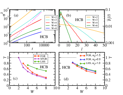
Figure 2: a) Spread $\sigma^{2}(t)$, evaluated for HCB with parameters as in Fig. 1b, b) corresponding averaged SP profile $\bar{p}_{l}(t)$, evaluated for fixed $t=50$, and for different $W=2-6$, c) (sub)diffusion exponents $\gamma$ vs. disorder $W$ as evaluated from FGR, simplified rates (SFGR), and via full simulation using LHS, respectively. d) $\gamma$ from FGR approach for different $\omega_{0}=1.5,2.0$ and shorter $t<100$ compared with LHS results for $\omega_{0}=1$.

Finally, Fig. 2c shows the comparison between exponents $\gamma$, as obtained for HCB case from different methods again for $\omega_{0}=g=1,t_{b}=0.4$ but varying disorder $W$: a) numerical simulations via LHS followed to distances $\sigma\sim 5$; b) the spread $\sigma^{2}(t)$ emerging from FGR and rate equations for size $L\sim 200$; and c) simplified equation (8) via extracting $\alpha$ from the tails of $I(\Gamma_{l})\propto\Gamma_{l}^{\alpha}$ for $10^{-4}<\Gamma_{l}<10^{-2}$ and taking into account the relation for classical random-walking, Machta (1985); Bouchaud and Georges (1989)

$$\gamma=2\alpha/(1+\alpha).$$ (19)

We can notice that the full and simplified FGR results do agree well, while $\gamma$ from the full many-body time evolution is still significantly larger. The quantitative disagreement partly emerges from restricting Eq. (18) to stritctly single-boson processes, whereby two-boson processes might also contribute. This can be effectively simulated by increasing $\omega_{0}$. We therefore present in Fig 3d the FGR results also for $\omega_{0}=1.5,2.0$ (and $t_{b}=0.6,0.8$, respectively) which reveal better match with numerics.

V Quasi-periodic potential.

In order to elucidate further the subdiffusion in the case of HCB, we compare results with the model with quasiperiodic potential, as actually realized in cold-atom experiments on optical lattices.Schreiber et al. (2015); Bordia et al. (2016); Lüschen et al. (2017) We choose it in the (Aubry-Andree) form $h_{i}=\sqrt{2/3}W\cos(2\pi q_{0}i+\psi_{0})$ which has the same standard deviation as the random one, where $q_{0}=(1+\sqrt{5})/2$ is a golden mean and $\psi_{0}$ an arbitrary phase. We note in Fig. 3a that the distribution $I(\Gamma_{l})$ is qualitatively different from a random potential in Fig. 1b. The difference emerges from correlated energies allowing for resonance contributions to $\Gamma_{l}$. This indicates that for quasi-periodic potential the long-time dynamics would be always diffusiveŽnidarič and Ljubotina (2018) even for large $W$ , although from $\sigma^{2}(t)$ in Fig. 3b this is expected to emerge for, e.g., $W=6,8$ only for extremely long $t\gg\bar{\tau}\gg 10^{2}$. It is quite clear that the same conclusion holds true also for a particle in the quasiperiodic potential coupled to noninteracting bosons. In the latter case, the multi-boson processes which are suppressed for HCB, additionally contribute to the diffusive transport in the long–time regime. Results (not presented here) for quasiperiodic potential and NB are qualitatively very similar to results shown in Fig. 3 for HCB.

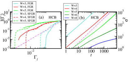
Figure 3: a) Distribution $I(\Gamma_{l})$ and b) spread $\sigma^{2}(t)$ for HCB with the same parameters as in Fig. 1b but for quasi-periodic potential.

VI Conclusions

The discussed model of SP moving in a 1D random potential is a prototype problem of quantum propagation in a disordered medium due to coupling to other (bosonic) dispersive degrees of freedom. We show that results obtained via the FGR represent an important simplification and insight, still they are nontrivial and appear to well (at least qualitatively) describe the whole many-body dynamics, as simulated numerically. First, due to the coupling to bosonic subsystem, the particle evolution is ergodic, approaching thermal equilibrium for $t\to\infty$. Still, a diffusive dynamics is not a rule. For noninteracting bosons it can appear only after transient subdiffusive spread $\sigma(t)\propto t^{\gamma}$ with $\gamma<1$, where time span of the latter regime strongly depends on the disorder $W$ and bosonic temperature $T$. Moreover, in the case of HCB our analysis and numerical results indicate that the subdiffusion persists at longest times, whereby the difference emerges due to multi-boson processes which are allowed for noninteracting bosons but are strongly suppressed for HCB. Still, beyond the energy conservation the character of SP wavefunctions are also crucial, as evident from the result that in a quasi-periodic potential the subdiffusion is only a transient phenomenonŽnidarič and Ljubotina (2018) also for HCB.

One cannot exclude that within a more accurate treatment of the multi-boson processes, the normal diffusion eventually sets on also in the HCB model. However, the crossover to normal diffusion will then happen at the time-scales which are much longer than for NB and, most probably, would be irrelevant for experiments.