An Optical Study of Two VY Sculptoris-Type Cataclysmic Binary Stars:
V704 And and RX J2338+431

Abstract

We report observations of the known cataclysmic variable star (CV) V704 And, and also confirm that the optical counterpart of the ROSAT Galactic Plane Survey source RX J2338+431 is a heretofore-neglected CV. Photometric and spectroscopic observations from MDM Observatory show both systems to be novalike variables that exhibit dips of 4-5 magnitudes from their mean brightnesses, establishing them as members of the VY Scl subclass. From high-state emission-line radial velocities, we determine orbital periods of 0.151424(3) d (3.63 hr) for V704 And and 0.130400(1) d (3.13 hr) for RX J2338+431. In V704 And, we find that the H$\alpha$ emission-line measures cluster into distinct regions on a plot of equivalent width versus full width at half-maximum, which evidently correspond to high, intermediate, and low photometric states. This allows us to assign spectra to photometric states when contemporaneous photometry is not available, an apparently novel method that may be useful in studies of other novalikes. Our low-state spectra of RX J2338+431 show features of an M-type secondary star, from which we estimate a distance of $890\pm 200$ pc, in good agreement with the Gaia DR2 parallax.

1 Introduction

Cataclysmic variable stars (CVs) are short-period binary star systems containing a white dwarf (WD) and a secondary that typically resembles a low mass main sequence star. The WD accretes mass as the secondary star overflows its Roche Lobe. CVs are classified by their photometric and spectroscopic properties into different subclasses. Those that remain mostly in a high state, with high mass transfer onto the WD, are classified as nova-like variables (NLs).

A subclass of NLs, VY Sculptoris stars, show occasional rapid drops in brightness by at least 1.5 magnitudes from their mean (Warner, 1995; Hellier, 2001). It is widely supposed Hellier (2001, and references therein) that VY Scl stars change states due to a variation in the mass transfer rate from the secondary. When the steady flow characteristic of the high state becomes disrupted, the accretion disk apparently vanishes and the low state of the system is observed. The cause of the mass-transfer rate variations is not known, but one proposed mechanism is the passage of a starspot on the secondary through inner Lagrangian point, at which the secondary loses mass. The lower temperatures in the star spot would decrease the photospheric scale height, suppressing the mass transfer.

In the low states of VY Scl stars, the broad emission lines commonly seen in CVs become weaker and much narrower. Also, the emission-line radial velocities in the low state can be up to 180 degrees out of phase with the high-state velocities (Warner, 1995). For more discussions on the low states of CVs, see Schneider et al. (1981); Shafter et al. (1985); Rodríguez-Gil et al. (2012).

In this paper, we present observations of two VY Scl stars, V704 And and RX J2338+431. Table 1 lists their basic properties.

V704 And, formerly known as LD 317, was first discovered by Dahlmark (1999) with a measured apparent V magnitude varying between 12.8 and 14.8. Papadaki et al. (2006) observed V704 And in 2003 September, 2003 November, and 2005 January and concluded the system had experienced fading episodes in 2003 and 2005. Our 2003 October observations showed the system in its high state, indicating the fade to the low state was rapid. This evolution is also seen in the American Association of Variable Star Observers (AAVSO) light curves, which show the star experiencing a fading event in late 2003 October into early 2003 November. The AAVSO light curves include observations of V704 And dating back to 1966, and show that there are multiple episodes of rapid drops in brightness ranging from 1 magnitude up to 4.5 magnitudes. This episodic fading behavior is consistent with other known VY Scl stars.

Table 1: Object Properties

Object Name	$\alpha$	$\delta$	2MASS			SDSS DR12					ROSAT
			J	H	K	g	u$-$g	g$-$i	r$-$i	i$-$z
	[h m s]	[$\arcdeg\ \arcmin\ \arcsec$]	(mag)	(mag)	(mag)	(mag)	(mag)	(mag)	(mag)	(mag)	(counts/sec)
V704 And	$23^{\rm h}44^{\rm m}57.5398^{\rm s}$	$+43\arcdeg 31\arcmin 22.318\arcsec$	12.892	12.714	12.579	$\cdots$	$\cdots$	$\cdots$	$\cdots$	$\cdots$	$0.03\pm 0.01$
RX J2338+431	$23^{\rm h}37^{\rm m}59.2213^{\rm s}$	$+43\arcdeg 08\arcmin 50.896\arcsec$	15.366	15.244	14.824	16.10	$-$0.07	0.08	0.09	0.08	$0.06\pm 0.02$

Note. —

Less has been reported on RX J2338+431 (Table 1). It was selected from the ROSAT Galactic Plane Survey (RGPS; Motch et al., 1991) as a hard X-ray source, and is listed in the ROSAT Bright Source Catalogue (1RXS J233801.0+430852; Voges et al., 1996). Direct imaging in 1999 October revealed an ultraviolet object at a location consistent with the ROSAT position (Table 2, Figure 1). Guided by the apparent UV excess from direct imaging, we obtained a spectrum of the UV-bright object on 1999 October 19 UT that showed emission lines consistent with a CV. We identify this object as the optical counterpart of 1RXS J233801.0+430852. The identification is noted in the online CV catalogs compiled by Downes et al. (2001) (see also Downes et al. 2005). The identification is corroborated by the Swift X-ray Point Source (SXPS) catalog (Evans et al., 2014), which lists a source only 0.6 arcsec from the optical counterpart.

Table 2: RX J2338+431 Photometry

Date	V	U$-$B	B$-$V	V$-$R
	(mag)	(mag)	(mag)	(mag)
October 1999	16.95	$-$1.00	$-$0.17	0.87
January 2000	20.07	$-$1.68	0.48	2.10
August 2008	16.50	$-$0.96	$-$0.03	0.73

Note. — June 2003 observations are not included because only V-band images were taking during that observing run.

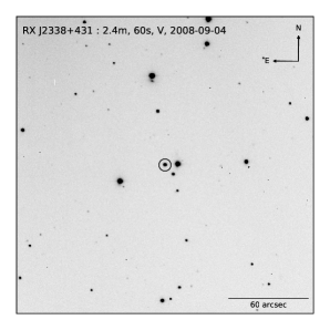
Figure 1: V-band exposure with the MDM 2.4m telescope from 2008 September 4 UT. The circle indicates the cataclysmic. North is at the top and east to the left, and the scale is indicated in the bottom right.

2 Observations

The spectral observations reported here are from the 2.4 m Hiltner telescope and the 1.3 m McGraw-Hill telescope at MDM Observatory on Kitt Peak, Arizona. At both telescopes, nearly all observations were taken with the “modspec” spectrograph with a $1\farcs 1$ slit and “Echelle” detector, a SITe $2048^{2}$ CCD giving a dispersion of 2 Å ${\rm pixel}^{-1}$ between 4210 and 7500 Å, with declining throughput toward the ends of the spectral range. When Echelle was unavailable a similar $1024^{2}$ SITe detector (“Templeton”) was used, which covered from 4660 to 6730 Å. For a few spectra we used the Mark III grism spectrograph, which covered 4580 to 6850 Å at 2.3 Å ${\rm pixel}^{-1}$ resolution. We used an incandescent lamp for a flat field, derived the wavelength calibration from observations of Hg, Ne, and Xe lamps, and observed flux standard stars in twilight when the weather was clear.

Spectral observations for V704 And were taken between 2001 January and 2016 June, and for RX J2338+431 between 1999 October and 2002 October. They cover the objects in their high, intermediate, and low states. Since all of our observations are from a single site, the sampling has an inevitable periodicity at $\sim 1$ sidereal day, which can lead to ambiguities in the daily cycle count. To ameliorate this problem, we took observations over a wide range of hour angle (Thorstensen et al., 2016). Tables 3 and 4 list the times of observation. Exposure were typically 480 s, but varied from 180 to 1200 s.

To reduce the spectra we used procedures based mostly on IRAF tasks; Thorstensen et al. (2016) and Thorstensen & Halpern (2013) give more detail.

Table 3: V704 And Radial Velocities

Time	$r_{\rm rad}$	$\sigma_{v}$	State
	[km s-1]	[km s-1]
52084.97272	12	3	H
52085.93072	$-$14	4	H
52086.84160	73	6	H

Note. — Table 3 is published in its entirety in the machine-readable format. A portion is shown here for guidance regarding its form and content.

Table 4: RX J2338+43 Radial Velocities

Time	$r_{\rm rad}$	$\sigma_{v}$	State
	[km s-1]	[km s-1]
51470.77543	$-$60	12	H
51470.77948	$-$52	14	H
51470.78637	$-$68	13	H

Note. — Table 4 is published in its entirety in the machine-readable format. A portion is shown here for guidance regarding its form and content.

For RX J2338+431, photometry was collected using the 2.4 m Hiltner telescope and Echelle CCD during 1999 October, 2000 January, 2003 June, and 2008 August. The magnitudes were calibrated with observations of Landolt (1992) standards. The error in the magnitude calibration is likely not to exceed $\sim 0.1$ mags as judged from the scatter in the standard star fits. Figure 2 shows the light curve, (blue circles), and Table 2 gives the colors.

We also synthesized $V$ magnitudes from our flux-calibrated spectra, by using a passband from Bessell (1990), and the IRAF sbands task, which multiplies the spectrum by the passband, integrates, and adds an appropriate constant. We often take spectra through thin cloud, and do not apply any correction for the light lost on the slit jaws (which varies with the seeing). The synthesized magnitudes are therefore less reliable and accurate than the filter photometry, which we only took under apparently clear skies and for which we used software apertures large enough to include the great majority of the light. Experience suggests that magnitudes synthesized from an average of several spectra are usually accurate to $\sim 0.3$ mag, when obviously poor spectra are excluded from the average.

3 Analysis

The emission-line radial velocities of VY Scl stars behave differently with photometric state, so in order to find the periods from radial velocities, we needed to create time series segregated by state. However, simultaneous photometry was not available for all our spectroscopic observations, and we were reluctant to rely on the less-accurate synthesized $V$ magnitudes, so we needed to determine the state without referring directly to magnitudes. To this end, we measured the equivalent width (EW, taken to be positive for emission) and full-width at half-maximum (FHWM, as determined from Gaussian fits) of the H$\alpha$ emission line. We then looked for correlations with the photometric states in cases where magnitudes were available.

Plots of the emission EW vs. the FWHM showed distinct groupings that proved to correspond to the photometric state, and we used these to separate the data into various states without reference to the photometric observations. For V704 And, three groupings emerged, which can be seen in Figure 3. The grouping with the smallest emission EWs (less than $\approx 51\,{\rm\AA}$) and FWHMa above $9\,{\rm\AA}$ (blue circles), corresponds to the photometric high state. Spectra in the group with FWHM less than $9\,{\rm\AA}$ (red squares) were from the low state, while those with EW above $\approx 51\,{\rm\AA}$ and FWHM greater than $12\,{\rm\AA}$ (green diamonds) were from an intermediate state. For RX J2238+431, only two groups emerged, which can be seen in Figure 3. The high state spectra had the highest FWHM above $15\,{\rm\AA}$ (blue circles), while the low state spectra had FWHM less than $15\,{\rm\AA}$ (red squares). As corroboration, we note that the groupings inferred from the EW vs. FWHM analysis corresponded well with the V-band magnitudes synthesized from the spectra (Figure 2).

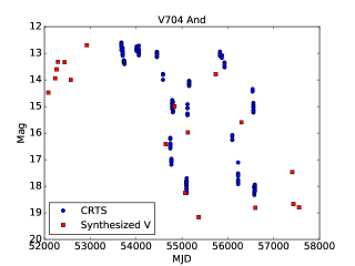
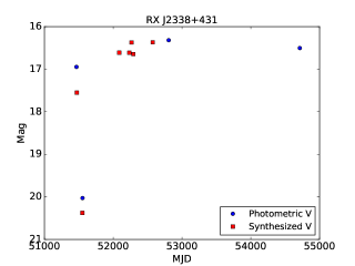
Figure 2: Light curves for V704 And (left) and RX J2338+431 (right). The red squares are the synthesized V magnitude determined from the spectral observations taken at MDM observatory. On the left, the CRTS Light Curve for V704 And is shown as blue circles. On the right, blue circles represent the observed V band magnitude from MDM photometric observations. RX J2338+431 is not covered by CRTS.

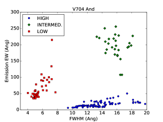
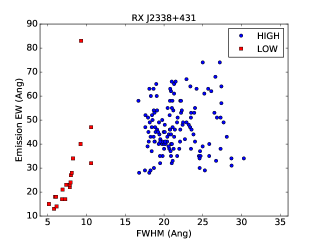
Figure 3: Emission equivalent width vs. full-width-half-maximum measurements of the H$\alpha$ emission line, which were used to classify the state of the CV. Left: V704 And, which has measurements in three states: high (blue circles), intermediate (green diamonds) and low (red squares). Right: RX J2338+431, which has measurements in two states: high (blue circles) and low (red squares).

For both the objects, the high-state spectra were the most numerous, so we used these to determine $P_{\rm orb}$. We measured H$\alpha$ emission radial velocities using a convolution algorithm (Schneider & Young, 1980), and applied a ‘residual-gram’ period search method described by Thorstensen et al. (2016). The middle panels of Figures 4 & 5 show periodograms for V704 And and RX J2338+431 respectively.

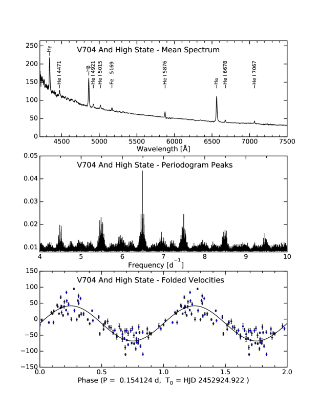
Figure 4: Average spectra, periodograms, and folded velocity curves for V704 And in the high state. The vertical scales, unlabeled to save space, are (1) for the spectra, $f_{\lambda}$ in units of $10^{-16}\textrm{ erg s}^{-1}\textrm{ cm}^{-2}\textrm{\AA}^{-1}$; (2) for the periodograms, $1/\chi^{2}$ (dimensionless); and (3) for the radial velocity curves, barycentric radial velocity in $\textrm{km s}^{-1}$. The periodogram is labeled with the word “peaks”, because the curve shown is formed by joining local maxima in the full periodogram with straight lines. This suppresses fine-scale ringing due to the unknown number of cycle counts between runs. The folded velocity curves all show the same data plotted over two cycles for continuity, and the best-fit sinusoid is also plotted. The velocities shown are H$\alpha$ emission velocities. The error bars for the emission lines are computed by propagating the estimated noise in the spectrum through the measurement, and hence do not include jitter from line profile variations.

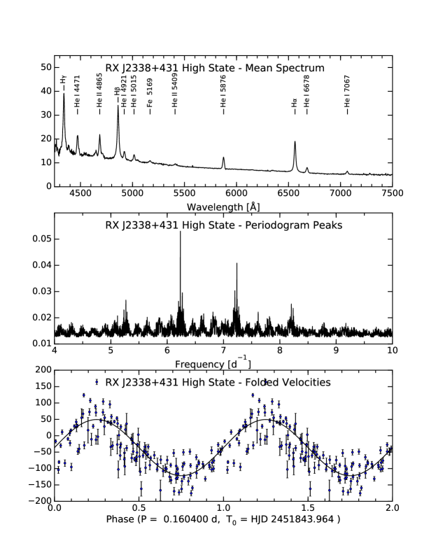
Figure 5: Similar to Figure 4 but for RX J2338+431 in the high state.

Fixing $P_{\rm orb}$ at the values determined from the high-state velocities, we fit sinusoids to the high-, mid-, and low-state velocities separately. The functional form of the fits was

$$v(t)=\gamma+K\sin{(2\pi(t-T_{0})/P)},$$ (1)

where $T_{0}$ is the Heliocentric Julian Date minus 2400000, and $P$ is the period in days (Table 5).

Table 5: Fits to Radial Velocities

Data set	$T_{0}$	$P$	$K$	$\gamma$	$N$	$\sigma$
		(d)	${\rm km\ s}^{-1}$	${\rm km\ s}^{-1}$		${\rm km\ s}^{-1}$
V704 And (High)	52924.2218(27)	0.154124(3)	55(4)	-13(3)	87	22
V704 And (Intermed.)	55128.7168(23)	$\cdots$	47(4)	-22(3)	31	19
V704 And (Low)	57430.5220(19)	$\cdots$	27(2)	-6(2)	47	9
RX J2338+431 (High)	51843.9642(25)	0.160400(1)	86(8)	-36(6)	135	35
RX J2338+431 (Low)	51553.6794(28)	$\cdots$	55(6)	-31(4)	19	28

Note. — Parameters of least-squares sinusoid fits to the radial velocities of the form $v(t)=\gamma+K\sin{(2\pi(t-T_{0})/P)}$.

4 Results

4.1 V704 And

The light curve of V704 And from the Catalina Real-time Transient Survey (CRTS) (Drake et al., 2009), Figure 2 (blue circles), shows repeated dimmings of $\sim 5$ mag. Additionally, Figure 2 shows good agreement between the V magnitudes synthesized from our spectra and the observed photometric light curve.

The high state spectrum (top panel Figure 4) shows Balmer emission lines and emission from He I $\lambda\lambda$ 4471, 4921, 5015, 5876, 6678, and 7067 as well as weak emission from an Fe blend at $\lambda$5169. In the intermediate state (top panel Figure 6), the continuum flux has decreased, but the emission lines have become relatively stronger. In the low state, there was both an overall decrease in the continuum flux and decreased line emission (bottom panel Figure 6), with a markedly steeper Balmer decrement. The He I and He II lines are nearly absent, though a small trace of He I $\lambda 5876$ may be present. The wide H$\beta$ absorption in the low state appears to be from the white dwarf photosphere.

Comparing the spectral appearance to the V magnitudes synthesized from the spectral observations, we found that the high-state spectra corresponded to $12.7\leq V\leq 16$, intermediate state to $16.4\leq V\leq 18.3$, and the low state to $V=18.9\pm 0.2$. We do not have enough coverage to say whether the system was brightening or dimming when the intermediate-state spectra were taken.

The low state spectrum (bottom panel Figure 6) shows features of a late-type secondary star in the far red end, although most of the spectrum is dominated by the WD continuum. To estimate the secondary’s spectral type, we scaled spectra of stars of known spectral type and subtracted them from the observed spectrum, with the aim of canceling out the late-type star’s features and leaving a smooth continuum. This was complicated by an unusually poor flux calibration longward of 7000 Å and shortward of 4500 Å. With those caveats, our best estimate for the secondary’s spectral type is M3–M4, and the best scaling gave a secondary contribution equivalent to $V\sim 21$. The Gaia Data Release 2 (Gaia Collaboration et al., 2018), which was published as this paper was being revised, gives a parallax of $2.4652\pm 0.0589$ mas, which inverts to $406\pm 10$ pc.

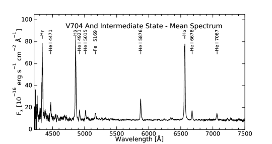
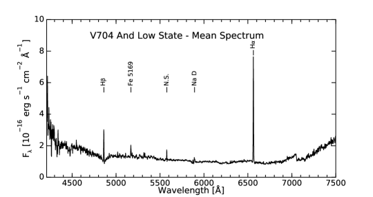
Figure 6: Average spectra for V704 And. Top: Average intermediate state spectrum from 2008 June. Bottom: Average low state spectrum from 2016 June. (There was apparently a problem with the flux calibration during the 2016 June observing run, and the continua longward of 7000Å and shortward of 4500Å are not reliable.) Noticeable differences can be seen between the spectra, including overall flux and lack of He I emission during the low state.

The periodogram of the high state radial velocities (middle panel Figure 4) reveals $P_{orb}=0.151424(3)\textrm{d}$, or $\sim 3.63$ hr. Periods that differ by one cycle per 9.5 years are considerably less likely but not entirely ruled out.

Folding all the velocities together on the orbital period reveals a clear phase shift between the velocities from the various states (Figure 7). The phase shift between the high and intermediate state is $0.80\pm 0.04$ while the shift between the high and low state is $0.52\pm 0.07$. This is not unprecedented; a phase shift between the high and low state of approximately 180 degrees is seen in TT Ari (Shafter et al., 1985).

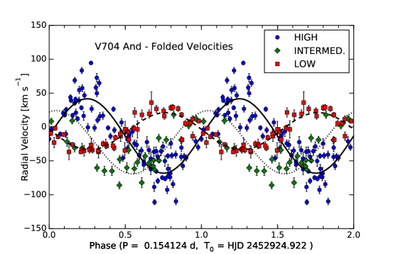
Figure 7: Folded velocity curves for V704 And in the high (blue circles), intermediate (green diamonds) and low (red squares) states. The curves all show the same data plotted over two cycles for continuity, and the best-fit sinusoid for each state is also plotted. The velocities shown are H$\alpha$ emission velocities.

4.2 RX J2338+431

The light curve from direct imaging shows RX J2338+431 changing states from high to low in 3 months between 1999 October and 2000 January (Figure 2). The 2000 October observations show it back in the high state.

In the high state, RX J2338+431 shows Balmer emission lines and emission from He I $\lambda\lambda$ 4471, 4921, 5015, 5876, 6678, and 7067, He II $\lambda\lambda$ 4685, 5409, as well as weak emission from an Fe blend at $\lambda 5169$ (top panel Figure 5). During the low state (Figure 8) the overall flux is much lower, and only narrow H$\alpha$ emission is present. H$\beta$ is not detected in emission or absorption, probably due to the poor signal-to-noise at $\lambda<5000$Å.

The low state average spectrum clearly shows a late-type contribution from the secondary star (Figure 8). We estimated the spectral type and flux of the secondary by subtraction, in a manner similar to that used for V704 And. For the type, we estimate M2.5$\pm$0.5, and the normalization corresponds to V $\sim 20.6$. Following the techniques described in Thorstensen & Halpern (2013), we used the observed flux and spectral type of the secondary, and a constraint on the secondary’s radius (derived from the orbital period and a plausible range for its mass), to estimate a distance of $890\pm 200{\rm\ pc}$. The Gaia Data Release 2 (Gaia Collaboration et al., 2018) parallax is $1.0742\pm 0.0722$ mas, corresponding to $d=930\pm 60$ pc, in excellent agreement with the photometric estimate.

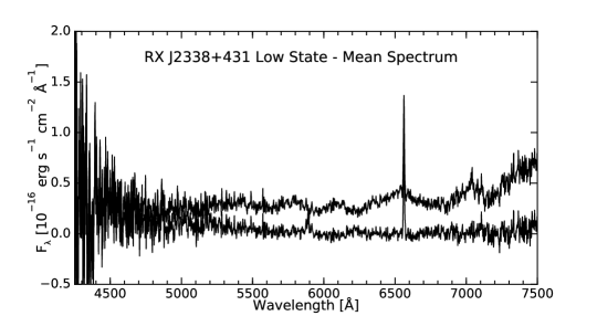
Figure 8: Average spectrum RX J2338+431 in the low state from 2000 January. The top trace shows the average spectrum, and the bottom shows the average spectrum after subtraction of a scaled M2.5-type spectrum.

The periodogram of the high state H$\alpha$ radial velocities (middle panel Figure 5) reveals $P_{orb}=0.160400(1)\textrm{ d}$, or $\sim 3.13$ hr. The likelihood of a cycle count error on day-to-day or run-to-run timescales is very small. When the radial velocities from high and low states are examined together (Figure 9) a phase shift of $0.25\pm 0.03$ is observed.

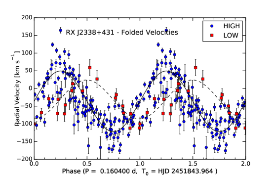
Figure 9: Folded H$\alpha$ emission velocity curves for RX J2338+431 in the high (blue circles) and low (red squares) states. The same data are shown repeated over two cycles for continuity, and the best-fit sinusoid for each state is also plotted.

5 Discussion

In many low state systems, there appears to be no evidence for emission from the disk. This is also the case for V704 And and RX J2338+431, as the emission lines that are seen are quite narrow, which is not consistent with the rotation broadening expected from a disk.

The origin of the narrow emission lines seen in the low states of VY Scl stars is poorly understood. Warner (1995) suggested that they could arise from irradiation of the secondary by the WD. If that were the case, the emission strength would be expected to vary with orbital phase, as the irradiated face rotates in and out of view (Thorstensen et al. 1978 present an early and clear-cut example of this phenomenon). In both of the systems studied here, the EW of the low-state H$\alpha$ does not vary systematically with phase, which would suggest that the emission comes from the whole surface, as from a chromosphere. However, the observed velocity amplitudes $K$ are much smaller than would be expected in this scenario; for plausible component masses, the observed $K$-velocities would require orbital inclinations $i$ less than $\sim 20\arcdeg$. For randomly oriented orbits, the probability of $i<20\arcdeg$ is only $0.06$, so the probability of finding two such systems at random is $0.06^{2}$ or 0.0036.

Several other VY Scl stars also show similarly puzzling behavior in their low-state H$\alpha$ emission. Schmidtobreick et al. (2012) present time-resolved VLT spectroscopy of the VY Scl star BB Dor in a low state. Their data are more extensive and have higher spectral resolution than ours, and show NaD emission lines that must arise on the secondary – they were able to trace the secondary’s motion by following a TiO band head, and the NaD emission was modulated similarly. They also detect narrow H$\alpha$ emission. Because they had traced the secondary’s motion independently, they established that the H$\alpha$ moves approximately in phase with the secondary, but with a significantly lower amplitude. (They also detect remarkable ‘satellite emission’ with velocities roughly consistent with gas orbiting near the L4 and L5 points; these do not appear in our data, perhaps because of our relatively modest signal-to-noise). Curiously, as in our data, they do not see an orbital modulation in the emission strength, as would be expected if the line originated at the heated face of the normal star. Rodríguez-Gil et al. (2012), in a study of the eclipsing VY Scl star HS0220+0603, similarly find that the modulation of the H$\alpha$ emission velocity has an amplitude $K\sim 100$ km s^-1, less than half that of the photospheric absorption at CaII (at $\lambda\lambda 8183,8194$). They suggest that the low H$\alpha$ velocity amplitude reflects an origin mostly on the facing hemisphere of the secondary. However, the H$\alpha$ line remains visible around zero (eclipse) phase, so the emission cannot arise entirely from the hemisphere facing the white dwarf. The sharpness, low velocity amplitude, and lack of orbital modulation of the H$\alpha$ line once again presents a puzzle.

The presence of relatively strong He II in the high state spectrum of RX J2338+431 suggests a magnetic system. X-ray selected CVs also tend to be disproportionately magnetic (Thorstensen & Halpern, 2013). The absence of dwarf nova outbursts during VY Scl low states provide indirect evidence for a magnetic field; Hameury & Lasota (2002) point out that according to disk instability theory, VY Scl stars in low states should show outbursts unless their disks are disrupted, as by a magnetic field . Time series photometry of RX J2338+431 might detect the regular pulsations characteristic of magnetic CVs (i.e. DQ Her stars or IPs).

6 Summary

We present photometric and spectroscopic observations of the cataclysmic variable systems V704 And and RX J2338+431. To our knowledge the optical identification of RX J2338+431 has previously appeared only in the Downes et al. (2001) catalog. We also describe a method to discriminate the different states of a VY Scl star system based upon the EW and FWHM of the H$\alpha$ line. Key findings about the two systems presented in this paper are as follows:

– Through spectroscopic observations spanning 15 years, we confirmed the VY Scl type classification of V704 And.

– Through photometry and spectroscopy, we identify RX J2338+431 as a CV of the VY Scl subclass.

– We determine the orbital periods to be $P_{orb}=0.151424(3)\textrm{ d}$ and $P_{orb}=0.160400(1)\textrm{ d}$ for V704 And and RX J2338+431, respectively, which fall in the period range typical of VY Scl novalikes.

– Phase shifts of $0.52\pm 0.07$ and $0.25\pm 0.03$ for V704 And and RX J2338+431, respectively, were found between the high and low states of the systems, indicating a change in the source of the emission line.

– Using the low state spectrum of RX J2338+431, we determine the secondary’s spectral type to be M2.5$\pm$0.5, and estimate a photometric distance of $890\pm 200{\rm\ pc}$, in good agreement with the nominally more accurate Gaia DR2 parallax.

References

- Alam et al. (2015) Alam, S., Albareti, F. D., Allende Prieto, C., et al. 2015, ApJS, 219, 12
- Bessell (1990) Bessell, M. S. 1990, PASP, 102, 1181
- Cutri et al. (2003) Cutri, R. M., Skrutskie, M. F., van Dyk, S., et al. 2003, VizieR Online Data Catalog, 2246
- Dahlmark (1999) Dahlmark, L. 1999, Information Bulletin on Variable Stars, 4734, 1
- Doi et al. (2010) Doi, M., Tanaka, M., Fukugita, M., et al. 2010, AJ, 139, 1628
- Downes et al. (2001) Downes, R. A., Webbink, R. F., Shara, M. M., et al. 2001, PASP, 113, 764
- Downes et al. (2005) Downes, R. A., Webbink, R. F., Shara, M. M., et al. 2005, Journal of Astronomical Data, 11, 2
- Drake et al. (2009) Drake, A. J., Djorgovski, S. G., Mahabal, A., et al. 2009, ApJ, 696, 870
- Evans et al. (2014) Evans, P. A., Osborne, J. P., Beardmore, A. P., et al. 2014, ApJS, 210, 8
- Gaia Collaboration et al. (2016a) Gaia Collaboration, Prusti, T., de Bruijne, J. H. J., et al. 2016, A&A, 595, A1
- Gaia Collaboration et al. (2016b) Gaia Collaboration, Brown, A. G. A., Vallenari, A., et al. 2016, A&A, 595, A2
- Gaia Collaboration et al. (2018) Gaia Collaboration, Brown, A. G. A., Vallenari, A., et al. 2018, A&A, 616, A1
- Gänsicke et al. (1999) Gänsicke, B. T., Sion, E. M., Beuermann, K., et al. 1999, A&A, 347, 178
- Hameury & Lasota (2002) Hameury, J.-M., & Lasota, J.-P. 2002, A&A, 394, 231
- Hellier (2001) Hellier, C. 2001, Cataclysmic Variable Stars, Springer
- King & Cannizzo (1998) King, A. R., & Cannizzo, J. K. 1998, ApJ, 499, 348
- Landolt (1992) Landolt, A. U. 1992, AJ, 104, 340
- Motch et al. (1991) Motch, C., Belloni, T., Buckley, D., et al. 1991, A&A, 246, L24
- Papadaki et al. (2006) Papadaki, C., Boffin, H. M. J., Sterken, C., et al. 2006, A&A, 456, 599
- Rodríguez-Gil et al. (2012) Rodríguez-Gil, P., Schmidtobreick, L., Long, K. S., et al. 2012, Mem. Soc. Astron. Italiana, 83, 602
- Schmidtobreick et al. (2012) Schmidtobreick, L., Rodríguez-Gil, P., Long, K. S., et al. 2012, MNRAS, 422, 731.
- Schneider & Young (1980) Schneider, D. P., & Young, P. 1980, ApJ, 238, 946
- Schneider et al. (1981) Schneider, D. P., Young, P., & Shectman, S. A. 1981, ApJ, 245, 644
- Shafter et al. (1985) Shafter, A. W., Szkody, P., Liebert, J., et al. 1985, ApJ, 290, 707
- Thorstensen et al. (2016) Thorstensen, J. R., Alper, E. H., & Weil, K. E. 2016, AJ, 152, 226
- Thorstensen et al. (1978) Thorstensen, J. R., Charles, P. A., Margon, B., et al. 1978, ApJ, 223, 260
- Thorstensen & Halpern (2013) Thorstensen, J. R., & Halpern, J. 2013, AJ, 146, 107
- Truemper (1982) Truemper, J. 1982, Advances in Space Research, 2, 241
- Voges et al. (1996) Voges, W., Aschenbach, B., Boller, T., et al. 1996, IAU Circ., 6420, 2
- Warner (1995) Warner, B. 1995, in Cataclysmic Variable Stars, Cambridge University Press, New York